Full-order mode analysis within a mutilated relaxation time approximation

Abstract

In this paper, a detailed normal mode analysis is given based on the Boltzmann equation in mutilated relaxation time approximation (RTA). Within this linearized effective kinetic description, our analysis covers a full-order calculation in wavenumber $k$, being a generalization of usual hydrodynamic mode analysis to intermediate and short-wavelength region. Besides, the proposed normal mode analysis can give a natural classification of kinetic modes into collective modes and non-collective single particle excitations. In the case with a scale-independent relaxation time, the so-called behavior of hydrodynamic onset transitions is recovered [1]. However, for a general case with a scale dependent relaxation time, a clear classification broken down because the location of hydrodynamic modes is not well separated from non-hydrodynamic modes.

I Introduction

As a universal effective theory of large distance and time scale, relativistic hydrodynamics has been widely applied to high energy physics [2] and cosmology [3]. Recently, relativistic hydrodynamics has found successful application in characterizing the evolution of the fireball generated during relativistic heavy-ion collisions. It has been instrumental in deducing the properties of Quantum Chromodynamics (QCD) matter, quark-gluon plasma (QGP), through the analysis of experimental data generated at BNL-RHIC and CERN-LHC [4, 5, 6, 7, 8, 9, 10, 11]. Surprisingly, a hydrodynamic model can seemingly rule everything all considering its unexpected success in describing the dynamic evolution of small system such as nucleus-nucleon and possibly proton-proton collisions [12, 13], which raises a thought-provoking question of when and how hydrodynamics emerges from a kinetic description in a non-equilibrium system.

Though the community of heavy-ion collisions has long made it a rule to employ hydrodynamics as a tool for quantitatively explaining experimental results, a thorough understanding of its application range is still lacking and deserves further investigation. In phenomenological modeling of relativistic heavy-ion collisions, the system must go through a very fast equilibration in order to better simulate the evolution of created QGP and fit well to the experimental data. However, this still remains an unsettled open question of how thermal equilibrium in relativistic heavy-ion collisions is reached so quickly. Generally speaking, understanding the establishment of thermalization in a physical system initially far from equilibrium is of fundamental importance in various regions. Regarding this issue, the attractor structure commonly known in complex physics is recently identified in the context of relativistic hydrodynamics, which could offer a reasonable qualitative explanation for the applicability of hydrodynamic models even on short time scales. There are also many efforts along this line to attempt to gain insight into the relationship between the attractor behavior and early-time dynamics [14, 15, 16, 17, 18, 19, 20].

It is widely accepted that relativistic hydrodynamics is only an effective description of a dynamic system in the limit of long wavelengths and late times. For a system driven out of equilibrium, a full kinetic description should be adopted to capture the properties of non-equilibrium physics. As the system gradually evolves to a near-equilibrium state, the hydrodynamic behavior emerges and is responsible for subsequent late-time evolution. There are successful practices where hydrodynamics can grow out of a kinetic description by using the techniques of gradients expansion such as Chapman-Enskog expansion and moment expansion, see [21] and reference therein.

As mentioned above, it should be a good starting point to use kinetic description to study both far-from equilibrium and near equilibrium behaviors and extract their close relation. In this work, we utilize an effective relativistic kinetic theory to do this. The linearized Boltzmann equation in the mutilated relaxation time approximation is taken as our main equation and the normal mode solutions are sought. Our detailed normal mode analysis covers a full-order calculation in wavenumber $k$, generalizing the usual hydrodynamical analysis to intermediate and short-wavelength region. Considering that hydrodynamization is always understood as the emergence of hydrodynamic modes with the decay of non-hydrodynamic modes, our research here can help to understand the related physics. The organization of this paper is put as follows. In Sec. II we give a short review of the linearized kinetic equation. In Sec. III, a transport model with a mutilated relaxation time is constructed. The advantages of this model over transitional RTA are also elaborated. Sec. IV is devoted to our main analysis. Here we take a scale-independent relaxation time and carry out a full-order normal mode analysis. With hydrodynamic modes and non-hydrodynamic modes classified and identified, the onset transition behavior is recovered. When the same analysis is applied to a case with a scale-dependent relaxation time in Sec. V, the inseparability of hydrodynamic modes and non-hydrodynamic modes is founded. Their interplay brings complexity to late-time dynamic evolution. Summary and outlook are given in Sec. VI. We have also put some related materials into appendix. Natural units $k_{B}=c=\hbar=1$ are used. The metric tensor here is given by $g^{\mu\nu}=\operatorname{diag}(1,-1,-1,-1)$ , while $\Delta^{\mu\nu}\equiv g^{\mu\nu}-u^{\mu}u^{\nu}$ is the projection tensor orthogonal to the four-vector fluid velocity $u^{\mu}$. The abbreviation dP stands for $\int dP\equiv 2\int d^{4}p\,\delta(p^{2}-m^{2})$. In addition, we employ the symmetric shorthand notations $X^{(\mu\nu)}\equiv(X^{\mu\nu}+X^{\nu\mu})/2$.

II Linearized kinetic equation

The non-equilibrium evolution of a relativistic system is dictated by relativistic Boltzmann equation,

$$(p\cdot\partial+F\cdot\partial_{p})f(x,p)=C[f],$$ (1)

where one-particle distribution function $f$, function of phase space point $(x,p)$, is crucial in relativistic kinetic theory, from which other physical observables or quantities can be obtained via phase space integration. The symbols $\partial$ and $\partial_{p}$ are used to denote the partial derivative with respect to the coordinate $x$ and particle momentum respectively, and $F$ is the external force exerted on the particles and will be set zero from now on. Last but not the least, $C[f]$ is called the collision term, namely, describing how the distribution function $f$ is affected by the local collisions between particles,

$$C[f]\equiv\; \int dP^{\prime}dP_{1}dP_{2}\big{(}f(p_{1})f(p_{2})\tilde{f}(p)\tilde{f}(p^{\prime})-f(p)f(p^{\prime})\tilde{f}(p_{1})\tilde{f}(p_{2})\big{)}W_{p,p^{\prime}\to p_{1},p_{2}},$$ (2)

where we have invoked the detailed balance property $W_{p,p^{\prime}\to p_{1},p_{2}}=W_{p_{1},p_{2}\to p,p^{\prime}}$ for the transition rate and $\tilde{f}=1\pm f$ with $-$ for fermions and $+$ for Bosons is implied. In the limit of classical statistics, $\tilde{f}$ is trivially $1$ and we will only focus on this case. Only two body collisions are considered now. Note that (1) is only one-component version of Boltzmann equation and one can see [21, 22] for a detailed discussion for a general multi-component system.

Due to nonlinearity of the collision term, the integro-differential equation (1) is hard to be solved completely. Then one often turns to some practically useful techniques to linearize the Boltzmann equation, among which Chapman-Enskog expansion and moment expansion are thought to be standard methods [21]. In the long wavelength limit where the mean free path $\ell_{\text{mfp}}$ of the system is small compared to the typical length $L$ associated with system non-uniformity, hydrodynamics can be developed from kinetic theory via Knudsen number ($\frac{\ell_{\text{mfp}}}{L}$) expansion.

To proceed, we note after the linearization the resulting transport equation is,

$$p\cdot\partial\chi(x,p)=-\mathcal{L}\chi(x,p),$$ (3)

with the linearized collision operator

$$\mathcal{L}[\chi]\equiv\int dP^{\prime}dP_{1}dP_{2}f_{leq}(p)f_{leq}(p^{\prime})\big{(}\chi(p_{1})+\chi(p_{2})-\chi(p)-\chi(p^{\prime})\big{)}$$ (4)

where an expansion is made according to $f=f_{leq}(1+\chi)$ with a local equilibrium distribution defined as

$$f_{leq}(p)=\frac{1}{(2\pi)^{3}}\exp[\xi-\beta\cdot p].$$ (5)

Here $\beta^{\mu}\equiv\frac{u^{\mu}}{T},\xi\equiv\frac{\mu}{T},\beta\equiv\frac{1}{T}$ with the temperature $T$, and the chemical potential $\mu$ introduced for conserved particle number. By construction, the local equilibrium distribution will put the right hand side (RHS) of the transport equation zero $C[f_{leq}]=\mathcal{L}[f_{leq}]=0$, because $1$ and $p$ are collision invariants. Under some limited circumstance, the left hand side (LHS) of the transport equation is also zero $p\cdot\partial f_{leq}=0$. This special state of local equilibrium is called global equilibrium, in which state we have

$$\partial_{(\mu}\beta_{\nu)}=0,\quad\xi=\text{const},$$ (6)

Moving back to the linearized Boltzmann equation (3), $\mathcal{L}$ is positive semidefinite interpreted as a linear operator in square integrable Hilbert space. Moreover, $\mathcal{L}$ respects the following property,

$$\mathcal{L}[\psi]=0,\quad\psi=a+b\cdot p$$ (7)

with $a$ and $b^{\mu}$ being the free parameters independent of $p$. Note collision invariants are the only zero modes in the eigen spectrum of $\mathcal{L}$. In fact, the structure of the linearized Boltzmann equation resembles time-dependent Schrodinger equation. Likewise, a thorough understanding of the ”energy” spectrum of $\mathcal{L}$ is necessary to deal with the evolution equation. Literally, solving the eigen spectrum of $\mathcal{L}$ is almost equivalent to settling the linearized transport equation. However, as far as we are concerned, the only analytical eigen spectrum are obtained by C.S.Wang Chang and U.E.Uhlenbeck in the context of monatomic gases in the non-relativistic case (see chapter IV of [23]).

Attacking the problem of solving the eigen spectrum of $\mathcal{L}$ is a rather ambitious task. If not insisting on solving a linearized transport problem precisely, we are inclined to confining our discussion to a simplified collision operator. Consider temporarily an issue of momentum isotropization despite the inhomogeneity smoothing that takes place far more slowly, and one can reduce (3) into a form of pure momentum transport,

$$p\cdot\partial\chi^{\prime}(p,t)=-\mathcal{L}\chi^{\prime}(p,t),$$ (8)

which can be formally solved

$$\chi^{\prime}(p,t)=e^{-\frac{\mathcal{L}t}{p^{0}}}\chi^{\prime}(p,0),$$ (9)

where $\mathcal{L}$ acts like an Liouville evolution operator. This equation conveys a very clear information: the deviation from equilibrium is exponentially decaying via particle collisions except for five zero modes. Thus, it is not necessary to seek all eigen modes but finite ones as far as late-time dynamics are concerned.

III A model with a mutilated relaxation time

Guided by the principle put forward above, one can approximate the full linearized collision operator with a mutilated operator (see chapter V of [23] and discussions therein),

$$-\mathcal{L}\sim\big{(}-\gamma+\gamma\sum_{n=1}^{5}|\lambda_{n}\rangle\langle\lambda_{n}|\big{)}$$ (10)

with $|\lambda_{n}\rangle$ being five degenerate orthonormal eigenfunctions of $\mathcal{L}$ and $\gamma$ being a representative negative eigenvalue. This is nothing but a truncated eigen spectral expansion of $-\mathcal{L}$. The right hand side of Eq.(10) undoubtedly inherits an important and necessary property of $\mathcal{L}|\lambda_{n}\rangle=0,n=1,\cdots 5$. One may keenly observe that this is nothing but a kind of relaxation time approximation (RTA) by identifying $\gamma$ as the relaxation time $\tau_{R}^{-1}$. Compared to traditional RTA, the presence of extra counter terms retrieves the important property of collision invariants. The advantage of this improvement will become manifestly useful as will be shown later. On the other hand, $\mathcal{L}|\lambda_{n}\rangle=\gamma|\lambda_{n}\rangle,n>5$. This is what the name ”mutilated” comes from : all negative eigenvalues collapse into the largest negative eigenvalue.

Another advantage over traditional RTA is that the relaxation time is allowed to possess momentum dependence as it should do generally, which can also be easily seen from the structure of the full linearized collision operator. As for traditional RTA, other constrain conditions must be imposed to reconcile the momentum dependence of the relaxation time with the conservation laws. For instance,

$$\partial_{\mu}T^{\mu\nu}=-\int dP\frac{p^{\nu}u\cdot p}{\tau_{R}(u\cdot p)}f_{leq}\chi$$ (11)

is not naturally zero. Here $\tau_{R}(u\cdot p)$ should not be confused with $\tau_{R}\times(u\cdot p)$ and the kinetic definition of the energy-momentum tensor has been employed

$$T^{\mu\nu}\equiv\int dPp^{\mu}p^{\nu}f(x,p).$$ (12)

This conflict disappears when the relaxation time is momentum independent by imposing Landau matching conditions

$$\int dPp^{\nu}u\cdot pf_{leq}\chi=0.$$ (13)

Obviously, the conventional Landau matching conditions are in contradiction with a momentum dependent relaxation time limiting the application of traditional RTA. One compromise is that two conditions Eqs.(11) and (13) have to be met simultaneously. Instead of causing complication with two conditions, the mutilated RTA naturally incorporates all collision invariants, which on integration are exact expressions of conservation laws. This improvement also leaves space for different matching conditions from Landau type. We note a mutilated RTA is widely used in nonrelativistic kinetic theory and recently there are some relevant discussions in relativistic contexts [24, 25, 26].

To put Eq.(10) into a less-abstract form, a proper definition of the inner product is indispensable. Before that, we want to seek a solution of the form, $\chi\sim\tilde{\chi}(k,p)e^{-ik\cdot x}$, then the substitution of the expansion of $f$ into Eq.(3) leads us to

$$\tau\omega\tilde{\chi}+\hat{p}^{\mu}\kappa_{\mu}\tilde{\chi}=-iL\tilde{\chi},$$ (14)

where $L\tilde{\chi}\equiv\gamma\tau\big{(}\tilde{\chi}-\sum_{n=1}^{5}(\tilde{\psi}_{n},\tau\tilde{\chi})\tilde{\psi}_{n}\;\big{)}$ with notations

$$\tau\equiv\frac{p\cdot u}{T},\quad\omega\equiv\frac{u\cdot k}{n\sigma(T)},\quad\hat{p}\equiv\frac{p}{T},\quad\kappa^{\alpha}\equiv\frac{\Delta^{\alpha\beta}k_{\beta}}{n\sigma(T)},\quad\kappa\equiv\sqrt{-\kappa\cdot\kappa},\quad l^{\alpha}\equiv\frac{\kappa^{\alpha}}{\kappa},$$ (15)

where $\sigma(T)$ is an arbitrary constant with the dimension of cross sections. Here the inner product is defined as

$$(B,C)=\frac{1}{(2\pi)^{3}}\int dP\exp(\xi-\beta\cdot p)B(p)C(p).$$ (16)

The connection with Eq.(10) can be made clear by translating $\tilde{\psi}_{n}$ and $(\psi_{n},\tau\psi_{m})$ into $|\lambda_{n}\rangle$ and $\langle\lambda_{n}|\lambda_{m}\rangle$. The specific expressions for $\tilde{\psi}_{n}$ are determined according to the technique of Schmit orthonomalization and given as

$$\tilde{\psi}_{1}=\frac{1}{\sqrt{V_{1,1}}},\quad\tilde{\psi}_{2}=\frac{\beta(u\cdot p-\frac{e}{n})}{\sqrt{V_{2,2}}},\quad\tilde{\psi}_{3}=\frac{\beta l\cdot p}{\sqrt{V_{3,3}}},\quad\tilde{\psi}_{4}=\frac{\beta j\cdot p}{\sqrt{V_{3,3}}},\quad\tilde{\psi}_{5}=\frac{\beta w\cdot p}{\sqrt{V_{3,3}}},$$ (17)

where we have introduced a triad $(l,j,w)$ to form an orthonormal set of unit vectors with $u$. One can justify that the basis are orthonormal in the sense of

$$(\tilde{\psi}_{i},\tau\tilde{\psi}_{j})=\delta_{ij}.$$ (18)

When we work in rest frame $u=(1,0,0,0)$, this triad then denotes the set of unit vectors projecting onto $z,x,y$ directions. For simplicity, we put $u=(1,0,0,0)$ in the remainder of this paper. The normalization factors appearing in the above equation are given in the Appendix.B.

IV Scale-independent relaxation time and onset transition

In this section, we perform a full-order normal mode analysis, namely, our discussion is not limited to long wavelength range. The discussion parallels a similar calculation for retarded correlators given in [1]. In line with the similar analysis, we take the same basic settings and assume that the particles are massless so that some complicated momentum integrals can be analytically sought or at least greatly simplified. In some relevant physical systems such as quark gluon plasmas produced in ultra-relativistic heavy-ion collisions, the constituent particles in the media are thought as massless. One can surely loose the ultra-relativistic limitation to count for massive transport.

We first define fluctuation amplitudes accordingly,

$$\rho_{n}(k)\equiv(\tilde{\psi}_{n},\tau\tilde{\chi}(k,p)\,),$$ (19)

except for $n=2$

$$\rho_{2}(k)\equiv(\frac{\tau}{\sqrt{V_{22}}},\tau\tilde{\chi}(k,p)\,),$$ (20)

then the Fourier transformed linearized kinetic equation Eq.(14) turns into

$$(c+\frac{\hat{p}}{\tau}\cdot l)\tilde{\chi}=\hat{\gamma}\sum_{n=1}^{5}\rho_{n}\bar{\psi}_{n},$$ (21)

where the following notations are introduced

$$c\equiv\frac{-i\omega+\gamma}{-i\kappa},\quad\,\hat{\gamma}\equiv i\frac{\gamma}{\kappa}.$$ (22)

Here an important assumption that $\gamma$ is scale independent is made. In order to get $\tilde{\chi}$, the reciprocal of $(c+\frac{\hat{p}}{\tau}\cdot l)$ is needed (by using sphere coordination and calibrating the direction of $\kappa$ with $z$ direction without loss of generality, one can write $\frac{\hat{p}}{\tau}\cdot l$ as $\cos\theta$). Therefore, we must distinguish two distinct cases.

IV.1 Collective modes

If the factor of $(c+\cos\theta)$ is not zero, then the reversion can be made safely

$$\tilde{\chi}=\frac{\hat{\gamma}\sum_{n=3}^{5}\rho_{n}\tilde{\psi}_{n}}{c+\cos\theta}+\frac{\hat{\gamma}\rho_{1}(\tilde{\psi}_{1}-\frac{\beta^{2}e\sqrt{V_{11}}}{nV_{22}}u\cdot p+\frac{\beta^{2}e^{2}\sqrt{V_{11}}}{n^{2}V_{22}})}{c+\cos\theta}+\frac{\hat{\gamma}\rho_{2}(\frac{\beta u\cdot p}{\sqrt{V_{22}}}-\frac{\beta e}{n\sqrt{V_{22}}})}{c+\cos\theta},$$ (23)

where we have reorganized the expansion basis such that $\bar{\psi}_{1}=\tilde{\psi}_{1}-\frac{\beta^{2}e\sqrt{V_{11}}}{nV_{22}}u\cdot p+\frac{\beta^{2}e^{2}\sqrt{V_{11}}}{n^{2}V_{22}}$ and $\bar{\psi}_{i}=\tilde{\psi}_{i}$ for $i\neq 1$. This reorganization originates from the inconsistency between the energy density fluctuation amplitude $\rho_{2}$ and $\tilde{\psi}_{2}$. The definition of $\rho_{2}$ is different from the ones of other fluctuation amplitudes apparently.

Substituting Eq.(23) into Eq.(19), we have

$$\rho_{1} =\sum_{i=1}^{5}\frac{\exp(\xi)\rho_{i}}{(2\pi)^{3}\sqrt{V_{1,1}}}\int dP\exp(-\beta u\cdot p)\frac{\hat{\gamma}\tau\bar{\psi}_{i}}{c+\cos\theta}=\hat{\gamma}\coth^{-1}c\rho_{1}+\frac{3\hat{\gamma}\big{(}1-c\coth^{-1}c\big{)}}{2}\rho_{3},$$ (24)

$$\rho_{2} =\sum_{i=1}^{5}\frac{\exp(\xi)\rho_{i}}{(2\pi)^{3}\sqrt{V_{2,2}}}\int dP\exp(-\beta u\cdot p)\frac{\hat{\gamma}\tau^{2}\bar{\psi}_{i}}{c+\cos\theta}=\hat{\gamma}\coth^{-1}c\rho_{2}+2\sqrt{3}\hat{\gamma}\big{(}1-c\coth^{-1}c\big{)}\rho_{3},$$ (25)

$$\rho_{3} =\sum_{i=1}^{5}\frac{\exp(\xi)\rho_{i}}{(2\pi)^{3}\sqrt{V_{3,3}}}\int dP\exp(-\beta u\cdot p)\frac{\hat{\gamma}\tau^{2}x\bar{\psi}_{i}}{c+\cos\theta}=\frac{\sqrt{3}}{2}\hat{\gamma}\big{(}1-c\coth^{-1}c\big{)}\rho_{2}-3\hat{\gamma}c\big{(}1-c\coth^{-1}c\big{)}\rho_{3},$$ (26)

and

$$\rho_{4}=\rho_{5}=\sum_{i=1}^{5}\frac{\exp(\xi)\rho_{i}}{(2\pi)^{3}\sqrt{V_{4,4}}}\int dP\exp(-\beta u\cdot p)\frac{\hat{\gamma}\tau^{2}\sin\theta\cos\phi\bar{\psi}_{i}}{c+\cos\theta}=\frac{3}{2}\hat{\gamma}\rho_{4}\big{(}(1-c^{2})\coth^{-1}c+c\big{)}.$$ (27)

As can be seen from the above equations, $\rho_{1}$, $\rho_{2}$ and $\rho_{3}$ are mutually coupled to each other. Therefore, they constitute a closed linear equation set. Considering these fluctuation amplitudes are well defined in kinetic theory up to some trivial factors, we have to ensure their existence, or they should have meaningful solutions. In other words, the secular equation for this equation set has solutions

$$\Phi(\hat{\gamma},c)=\left(\hat{\gamma}\coth^{-1}c-1\right)\left(3\hat{\gamma}(c-\hat{\gamma})+(3c\hat{\gamma}(\hat{\gamma}-c)-\hat{\gamma})\coth^{-1}c+1\right)=0,$$ (28)

where $\Phi$ factorizes into a sound sector and a heat sector

$$\Phi_{1}(\hat{\gamma},c) =3\hat{\gamma}(c-\hat{\gamma})+(3c\hat{\gamma}(\hat{\gamma}-c)-\hat{\gamma})\coth^{-1}c+1=0,$$ (29)

$$\Phi_{2}(\hat{\gamma},c) =\hat{\gamma}\coth^{-1}c-1=0.$$ (30)

The difficulty of treating the secular equations lies in two free parameters. Even one of them $c$ is a complex. Before solving equations for these fluctuation amplitudes, the existence conditions for solutions should be figured out. This question is closely connected with the dispersion relations of hydrodynamic modes in intermediate and large wave numbers. At long wavelength, the existence and dispersion relations of hydrodynamic modes are well-known. To achieve this goal, we invoke a useful residue theorem (also called winding theorem) that the number of zeros of $\Phi$ in a region of the complex $c$-plane in which $\Phi$ is an analytic function is equal to the times of the representative point $\Phi$ in the $\Phi$-plane encircling the origin.

Let us treat $\Phi_{1}$ first. We choose to fix $\hat{\gamma}$ and move $c$ to see the track of running $\Phi_{1}$. Firstly, the asymptotic behavior of $c\rightarrow\infty$ is readily available

$$\Phi_{1}(\hat{\gamma},c\rightarrow\infty)=1,$$ (31)

when $\hat{\gamma}$ is finite, which renders drawing an accessible picture reality. Then $c$ runs along the upper real axis $c=a+i0^{+}$ and carry along the large semicircle . What we do is draw the picture of the path of $\Phi$ and see how many times the path wraps the origin. A typical diagram is displayed for $\hat{\gamma}=5$.

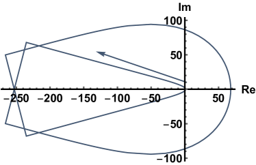
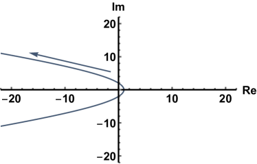
Figure 1: The typical trajectories of $\Phi_{1}(5,c)$. $\Phi_{1}$ starts from $1$ and anticlockwise encircles the origin for $3$ times while $c$ goes from $-\infty+i0^{+}$ to $\infty+i0^{+}$ and run across the large semicircle back to $-\infty+i0^{+}$. The right panel is an amplified version of the micro structure hidden in the left panel.

As is shown clearly in Fig.1, when $c$ runs along the boundary of upper complex plane, the trajectory of $\Phi_{1}$ encircles the origin three times corresponding to three collective modes known in relativistic hydrodynamics: one heat mode and two sound modes. One may have doubt about the broken lines that is not smooth appearing in the graph. That is where the branch points of $\Phi_{1}$ or $\coth^{-1}c$ are located: $c=\pm 1$. If increasing the density of data points near these branch points, the drawing curve shall be more smooth, but we needn’t bother ourselves with extra efforts, because a careful analysis on the asymptotic behavior of $\Phi_{1}$ near $c=\pm 1$ shows that the conclusion is unchanged as far as the net winding number is concerned. Note as an aside that when applying the winding theorem to the lower half plane of $c$, there are never zeros.

Then we want to investigate the short wavelength behavior of these collective modes. By lowering $\frac{\gamma}{\kappa}$ or increasing the value of $\kappa$, things gradually change. There will be a transition taking place at $\frac{\gamma}{\kappa}=0.2208$, below which two hydrodynamic sound modes have gone away, exhibited by the typical illustration in Fig.2. We note a similar study has been carried out in [1] where alike behavior is found and called hydrodynamic onset transition. The critical value for $\gamma$ is quite close to our result shown above: $\frac{\gamma}{\kappa}=0.2206$. A similar analysis applied to $\Phi_{2}$ indicates the same transition behavior for the heat mode with the critical value $\frac{\gamma}{\kappa}\simeq\frac{2}{\pi}$, below which the heat mode disappears. To be frank, our method of using winding theorem to determine the critical $\frac{\gamma}{\kappa}$ can only provide a numerical form. With reference to an analytical evaluation shown in [1], we confirm that the numerical value is in perfect agreement or precisely $\frac{2}{\pi}$. For comparison, we leave how this analytical calculation works to shear-channel modes afterwards. A more comprehensive comparation and some related comments will be given at the end of this section.

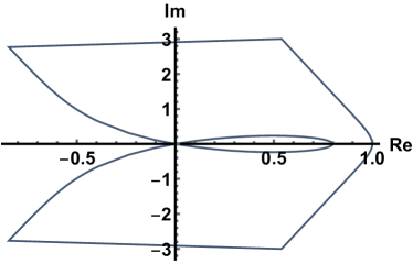
Figure 2: The typical trajectories of $\Phi_{1}(0.2208,c)$. The only intersection point lies on the right side of imaginary axis. The origin has never been enclosed.

Eventually, we move to shear-channel modes. The existence condition for (27)

$$\Phi_{3}(\hat{\gamma},c)=\frac{3}{2}\hat{\gamma}\big{(}(1-c^{2})\coth^{-1}c+c\big{)}-1=0.$$ (32)

We can repeat the above story to find the critical value for $\hat{\gamma}$ without any doubts and this gives us $\frac{\gamma}{\kappa}\simeq\frac{4}{3\pi}$. For the same reason, only an approximately equality is written. Then we introduce another analytical way to recalculate the critical value. To make it, we empirically admit a pure decaying dispersion relation $\omega=-i\gamma(1+\alpha(\kappa/\gamma)\,)$ for shear-channel modes, where $\alpha$ is a real function of $\kappa/\gamma$, then according to the definition of $c$, $c$ should be an imaginary value $c=-i\frac{\alpha(\kappa/\gamma)}{\kappa/\gamma}$. Then we have

$$(1+(\frac{\alpha}{\kappa/\gamma})^{2})\cot^{-1}[\frac{\alpha}{\kappa/\gamma}]-\frac{\alpha}{\kappa/\gamma}=-\frac{2}{3}\frac{\kappa}{\gamma}.$$ (33)

Luckily, $\frac{\alpha}{\kappa/\gamma}$ and $\frac{\kappa}{\gamma}$ decouple from each other without efforts. It is now physically reasonable to require that $\frac{\kappa}{\gamma}$ is positive. Therefore the critical value for shear channel transition $\frac{\gamma}{\kappa}$ is $\frac{4}{3\pi}$. With all the ingredients ready, the critical value for $\frac{\gamma}{\kappa}$ for various spin modes are numerically solved and displayed in Table. 1.

	Sound	shear	heat
winding theorem	0.2208	$\simeq\frac{4}{3\pi}$	$\simeq\frac{2}{\pi}$
empirical analytical calculation	0.2206	$\frac{4}{3\pi}$	$\frac{2}{\pi}$

Table 1: The critical value $\frac{\gamma}{\kappa}$ for various hydrodynamic modes in relativistic hydrodynamics. The precision of numerical calculation for ”$\simeq$” to hold is of the order $10^{-7}$.

Before ending this section, several comments are followed in order.

• The normal mode analysis presented here provides a way for full-order calculations in terms of wavenumber $\kappa$, being a generalization of hydrodynamic mode analysis [21, 27, 28, 29] to transient and short wavelength areas. Considering oversimplification of replacing the linearized collision kernel with a single relaxation time, the model can not offer a satisfying quantitative description, but we can take good use of it to study the analytical structure of hydrodynamics and provide insights into how hydrodynamic behavior grows or emerge from a kinetic theory. Notice that the counter terms appearing in Eq.(10) are very crucial, Eqs.(24) to (27) can’t be reached without them. This can be thought as another advantage of the novel RTA over the traditional one.

• In looking for normal modes hidden in Eq.(28) and (32) and determining the boundaries of onset transitions, no priori assumptions are made, in contrast to the procedure utilized in [1] where the author takes empirical forms for hydrodynamic dispersion relations. In this sense, it is preferable to turn to residual theorem. The application of both methods gives almost the same results, which can be seen as a cross check. Considering that we are careful with a control of numerical precision, the discrepancy, obvious but minor, in the critical value for the sound channel could be attributed from the fact that the empirical parameterization form of normal modes involved in the sound channel may not be always true. While for shear and heat channels, a good control of calculation precision up to $10^{-7}$ reveals the consistency of the parameterization form of normal modes showing up in these channels.

• The lack of the effects of sound-heat modes coupling should be noticed. At first glance, the sound and heat channels are mutually coupled to each other. However, they just trivially factorize just as shown in Eq.(29) and (30) as if the coupling appearing in Eq.(24) is a false. Furthermore, in the long wavelength limit, the equations governing the dispersion relations are indeed intertwined for sound modes and heat mode allowed by symmetry, which is widely seen in hydrodynamic calculations [27]. In order to elucidate the confusing point, we remind that two approximations are made in the process of calculation in practice: particles are massless and the relaxation time is taken to be energy-independent. If any one of these two assumptions are loosed, the entries of the coefficient matrix in Eqs.(24) to (26) are all nonzero in general. For instance, the calculations in non-relativistic limit are given in the page 207 of chapter V in [23], where all matrix elements are not zero. A verification for a scale-dependent relaxation time is also not hard to implement.

  The normal mode analysis presented naturally incorporates sound-heat modes coupling if we abandon any one of two approximations mentioned above. In the language of retarded correlators, taking the modes coupling into account means the cross retarded correlation functions such as $G^{R}_{ne},G^{R}_{en}$ should be additionally included, which calls for the calculations of $\frac{\delta T^{\mu\nu}}{\delta A^{\alpha}}$ and $\frac{\delta J^{\mu}}{\delta g^{\alpha\beta}}$ (please see specific definitions and notations in [1, 30]). In this sense, the normal mode analysis proposed here is more complete. Because of two simplifications brought by used approximations, these cross effects do little contributions to dispersion relations, so neglecting them in [1] accidentally causes no trouble.

IV.2 Non Collective modes

If the factor of $(c+\cos\theta)$ could be zero, equivalently, the real and imaginary parts of $\omega$ satisfy

$$\Re\omega\in[-\kappa,\kappa],\quad\Im\omega=-i\gamma,$$ (34)

which is nothing but the branch cut of $\Phi$ functions in the last subsection. We can obtain from Eq.(21)

$$\tilde{\chi}=A(\omega,\kappa)\delta(c+\cos\theta)+\hat{\gamma}\sum_{n=1}^{5}\rho_{n}\bar{\psi}_{n}\text{P}\frac{1}{c+\cos\theta},$$ (35)

where P represents the principal value, $A$ is an function whose form is left undetermined and $x\delta(x)=0$ has been utilized. For illustration, we only confine our discussion to sound-heat channels, and the substitution of Eq.(35) into the definition of $\rho_{i}$ will lead to a linear inhomogeneous equation

$$\rho_{1} =\frac{A}{2}+\hat{\gamma}\coth^{-1}c\rho_{1}+\frac{3\hat{\gamma}\big{(}1-c\coth^{-1}c\big{)}}{2}\rho_{3},$$ (36)

$$\rho_{2} =\frac{\sqrt{3}A}{2}+\hat{\gamma}\coth^{-1}c\rho_{2}+2\sqrt{3}\hat{\gamma}\big{(}1-c\coth^{-1}c\big{)}\rho_{3},$$ (37)

$$\rho_{3} =-\frac{3Ac}{4}+\frac{\sqrt{3}}{2}\hat{\gamma}\big{(}1-c\coth^{-1}c\big{)}\rho_{2}-3\hat{\gamma}c\big{(}1-c\coth^{-1}c\big{)}\rho_{3}.$$ (38)

where $c$ is taken to be $\frac{\Re\omega}{\kappa}$. With simple algebraic manipulations, these fluctuation amplitudes can be solved

$$\rho_{1} =\frac{A\left(\hat{\gamma}\coth^{-1}c\left(-9\hat{\gamma}c^{2}\coth^{-1}c+3c(5c+\hat{\gamma})+8\right)+6\hat{\gamma}^{2}-15c\hat{\gamma}-8\right)}{16\left(\hat{\gamma}\coth^{-1}c-1\right)\left(3\hat{\gamma}(c-\hat{\gamma})+\hat{\gamma}(3c(\hat{\gamma}-c)-1)\coth^{-1}c+1\right)},$$ (39)

$$\rho_{2} =\frac{\sqrt{3}A\left(3\hat{\gamma}c^{2}\coth^{-1}c-3\hat{\gamma}c-2\right)}{4\left(3\hat{\gamma}(\hat{\gamma}-c)+\hat{\gamma}(3c(c-\hat{\gamma})+1)\coth^{-1}c-1\right)},$$ (40)

$$\rho_{3} =\frac{3A\left(\hat{\gamma}c\coth^{-1}c+c-2\hat{\gamma}\right)}{8\left(3\hat{\gamma}(\hat{\gamma}-c)+\hat{\gamma}(3c(c-\hat{\gamma})+1)\coth^{-1}c-1\right)}.$$ (41)

Substituting these obtained fluctuation amplitudes $\rho_{i}$ back into Eq.(35), we get a explicit solution of normal mode problem. In this case, there is no functional relation, namely, dispersion law, between $\omega$ and $\kappa$ as a condition for the existence condition for collective modes. As signified by the delta function appearing in Eq.(35), these modes are exactly single-particle modes associated with a continuum single particle spectrum. In free-flow dominated region, we can set the linearized collision operator zero,

$$\tilde{\chi}\sim A(\omega,\kappa)\delta(c+\cos\theta),$$ (42)

the initial fluctuation is carried away by disordered particles thus there are no discrete kinetic modes and dispersion relations. All continuum modes all damped with a characteristic relaxation time $\gamma^{-1}$ according to Eq.(34).

IV.3 A complete description

In last two subsections, we have discussed the normal mode solutions of linearized kinetic theory. Formally, these normal modes can be grouped into two classes. The fist one consists of discrete kinetic modes with definite dispersion relations, which match hydrodynamic modes in the limit of long wavelength. To better explain it, we show how to identify their hydrodynamic dispersion relations through hydrodynamic expansion, taking the heat channel as an example. Recalling the definition of $c$, a hydrodynamic expansion around $\kappa=0$ would send $c$ to infinity, then the asymptotic behavior of $\coth^{-1}c$

$$\coth^{-1}c=\frac{1}{2}\ln\frac{c+1}{c-1}=\sum_{n=0}^{\infty}\frac{1}{2n+1}\frac{1}{c^{2n+1}}$$ (43)

can be utilized. When $|c|$ goes to infinity, a truncation of $\frac{1}{c}+\frac{1}{3c^{3}}+\mathcal{O}(\frac{1}{c^{5}})$ is used to replace $\coth^{-1}c$ in $\Phi_{2}$,

$$\Phi_{2}(\hat{\gamma},c)=\hat{\gamma}(\frac{1}{c}+\frac{1}{3c^{3}})-1=0,$$ (44)

after putting the expression of $c\equiv\frac{\omega+i\gamma}{\kappa}$ into $\Phi_{2}$, we reach $\omega=-i\frac{1}{3\gamma}\kappa^{2}+\mathcal{O}(\kappa^{4})$, which reproduces the well-known hydrodynamic dispersion relations of the heat mode.

By repeating the calculation procedures, the other hydrodynamic dispersion relations can be sought and collected as follows

$$\omega =\pm c_{s}\kappa-\frac{2i}{15\gamma}\kappa^{2},\quad\quad\text{sound modes}$$ (45)

$$\omega =-\frac{i}{3\gamma}\kappa^{2},\quad\quad\text{heat mode}$$ (46)

$$\omega =-\frac{i}{5\gamma}\kappa^{2},\quad\quad\text{shear modes, twofold degeneracy}$$ (47)

where the sound speed $c_{s}=\frac{1}{3}$ in its conformal limit. These are consistent with the number of zeros predicted by winding theorem. Therefore, we name various channels with their hydrodynamic correspondence. These kinetic modes grow out of the zero eigenvalues of the collision operator, reflecting the ways of ordered particle collective motion organized by collisions. A sharp-eyed reader may observe that there are some distinctions between our results reported here with those in [1] for the absence of extra non-hydrodynamic modes.

To fix this issue, a reminder is invoked that the equations Eqs.(29), (30) and (32) reproduce the denominators of corresponding retarded correlators formulated in [1] with careful and patient reduction works done. Thus, the zeros of Eqs.(29), (30) and (32) represent the hydrodynamic poles. Since the numerical analysis using residue theorem definitely tells us there are only five zeros, the extra non-hydrodynamic modes can only be ascribed to the approximation made or other cases beyond the reach of the winding theorem. Now we want to argue that these two possibilities are consistent with each other.

Irrespective of the numerator factors, we can also manufacture our own retarded correlators making the best of elements readily available, by naively reverse the the equations governing the dispersion relations, for instance, in the heat channel

$$G^{0,0}_{J}\sim\Phi_{2}^{-1}=\frac{1}{\hat{\gamma}\coth^{-1}c-1},$$ (48)

one can refer to [1] for relevant conventions used here. Then we apply $(2,2)$ type Pade approximation to $G^{0,0}_{J}$ around $\kappa=0$ and get

$$G^{0,0}_{J}\sim\frac{-\frac{3i\kappa^{2}}{5\omega(\gamma-i\omega)}-\frac{i(\gamma-i\omega)}{\omega}}{1+\frac{\kappa^{2}(9\omega+5i\gamma)}{15\omega(\gamma-i\omega)^{2}}}.$$ (49)

By analyzing the denominator of $G^{0,0}_{J}$, one can identify another two poles in the form of non hydrodynamic modes

$$\omega=-\frac{i}{\gamma}\pm\frac{2}{\sqrt{15}}\kappa+\mathcal{O}(\kappa^{2})$$ (50)

in accordance with the results given in [1]. In addition, we can also find two extra non hydrodynamic modes in shear channel

$$\omega=-\frac{i}{\gamma}\pm\frac{1}{\sqrt{7}}\kappa+\mathcal{O}(\kappa^{2}).$$ (51)

The application of Pade approximation is crucial to the presence of non hydrodynamic modes and even decides how many these modes are. Because the spirit of Pade approximation is to use the ratio of rational polynomials to approximate a complicated function, it shall bring in more poles as the order of Pade approximation increases. Such a similar finding is also reported in [1] when the author studies the strong coupling limit of retarded correlators.

On the other hand, these newly appearing non hydrodynamic modes are all falling into another class that will be introduced next. As is summarized in the last subsection, it is continuum single-particle modes that play the dominant role in free-flow region. The other class is composed of these normal modes. Note that their dispersion relations (though it may be inappropriate to continue to use this concept) are dictated by

$$\Re\omega\in[-\kappa,\kappa],\quad\Im\omega=-i\gamma,$$ (52)

where Eqs.(50) and (51) are precisely falling into this region. If increasing the order of Pade approximation to infinitely large, these non-hydrodynamic modes will spread over this branch cut, which lies out of the application range of winding theorem. To conclude, these non-hydrodynamic modes are nothing but non collective single-particle modes, associated with the branch cut of retarded correlators.

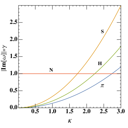
Figure 3: The imaginary parts of hydrodynamic modes as a function of $\kappa$. S, H, $\pi$ and N denote sound modes, heat mode, shear modes and non-hydrodynamic modes respectively.

Last but not the least, it is worth noting that the typical relaxation times for hydrodynamic and non-hydrodynamic modes are well separated. The presence of a momentum independent relaxation time set in a new scale or gap $\gamma$, shown by the red solid line in Fig.3. Only low energy (frequency) effective degrees of freedoms (DOF) lie below the gap contribute most to late-time dynamics. That is why we call hydrodynamics a low energy effective theory in the long wavelength limit. The sharpness of onset transitions is also due to the energy independence of the gap. In the next section, the interplay of collective hydrodynamic modes and non-collective non-hydrodynamic modes is displayed. In that case, the unique leading role of hydrodynamic modes in late-time evolution is challenged by non-hydrodynamic single-particle modes.

V Scale-dependent relaxation time and dehydrodynamization

As is put forward in Sec.III, the mutilated model naturally admits a scale-dependent relaxation time, i.e., we needn’t impose other conditions to ensure consistency. Generally, the relaxation time has momentum dependence. Hereafter, we focus on the impact of the scale dependence of relaxation time on the normal mode analysis carried out above.

Starting from Eq.(21), a minor change in the definition of $c$ and $\hat{\gamma}$ is made

$$c\equiv\frac{-i\omega+\gamma/\tau^{\lambda}}{-i\kappa},\quad\,\hat{\gamma}\equiv i\frac{\gamma}{\kappa\tau^{\lambda}}.$$ (53)

with other following expressions intact. In this case, the reciprocal of relaxation time is parameterized as energy dependent $\gamma\rightarrow\gamma/\tau^{\lambda}$ with the specific value of $\lambda$ relying heavily on the dynamic details and corresponding to various physical scenarios. For example, $\lambda=0$ corresponds to traditional Anderson and Witting (AW) RTA [31], into which we have put much effort in the last section. In addition, $\lambda=0.38$ is argued to well approximate the effective kinetic descriptions of quantum chromodynamics for it offers the best fit to part of experimental results [32, 33]. Since we are not intended to quantitatively fit the experimental data, the value of $\lambda$ is kept unspecified.

To proceed, we look back at Eq.(23). It is a necessary step to reverse Eq.(21) to get the formal expression of deviation function $\tilde{\chi}$ before collective kinetic modes can be identified. However, we should be careful with the reversion in that the LHS of Eq.(23) containing $c$ is dependent on $\tau$ ranging from zero to real infinity. Thus, $(c+\cos\theta)$ is potential zero, as long as

$$\Re\omega\in[-\kappa,\kappa],\quad\Im\omega=-i\gamma/\tau^{\lambda},$$ (54)

so we should not naively divide this factor.

Given a fixed $\tau$, the criteria of classification into collective modes and non collective single particle modes works as usual as long as the branch cut is shifting from Eq.(52) to Eq.(54). However, $\tau$ is not a fixed extern variable but a intermediate variable that will be integrated out. Varying $\tau$ will result in a collection of branch cut lines. For example, when treating the shear channel, we have to confront the following equation

$$\rho_{4}=\frac{i\gamma\rho_{4}}{16\kappa}\int d\tau\exp(-\tau)\tau^{4-\lambda}\big{(}(1-c^{2})\coth^{-1}c+c\big{)},$$ (55)

where $\tau$ is scanned from zero to infinity in the process of integration. When $\lambda$ is zero, the above equation consistently reduces to Eq.(27).

A integration over $\tau$ implies that we have not only one branch cut line but a strip made up of a series of branch cuts. This strip takes up the whole lower complex plane of $\omega$ with the real part of $\omega$ ranging from $-\kappa$ to $\kappa$. Besides, a $\tau$-scan renders a division by $(c+\cos\theta)$ illegal, so a classification, or more accurately, a separation of collective modes from non-collective single-particle modes is not feasible. This can be illustrated by visualizing Fig.3: when there is only a single branch cut line, we can identify the hydrodynamic modes below the branch line as low energy effective degrees of freedom. Now we can translate the non-hydrodynamic branch line up and down to fill this rectangle half plane, then all the hydrodynamic modes are embedding in this strip structure. Noting the single-particle mode with a larger energy has a smaller imaginary part, the most energetic single-particle modes are intertwined with hydrodynamic modes. There is no such a gap below which hydrodynamic modes are the only low energy degrees of freedom.

Let’s put the argument more mathematically. The integral in Eq.(55) is intractable and we decide to redo the calculation explicitly. For concreteness and simplicity, $\lambda$ is set to be $1$ and we only concentrate on the non-analytical structure in presence and discard unimportant factors. The to-do integral is of the form

$$I=\Big{(}-\partial_{a}\int_{-1}^{1}dx\int_{0}^{\infty}d\tau\frac{\exp(-a\tau)}{(\omega+\kappa x)\tau+i}\Big{)}_{a=1}$$ (56)

which matches exactly with an important integral formula calculated in a similar work and we refer the readers to [30] for more details. After carrying out $\tau$ integration and integrate by parts, this integral can be worked out

$$I\sim 2\pi i\exp(-1/\Im\omega)\theta(-\Im\omega)\theta(\kappa^{2}-\Re\omega^{2})$$ (57)

where we have only retained the mathematical result indicating the nonanalytic strip structure. This structure comes from the x-integration crossing the branch cut of incomplete gamma function $\Gamma[0,\frac{ia}{\omega+x}]$, which appears after $\tau$ integration is done. In a short summary, both Eq.(54) and (57) give the similar nonanalytic strip structure for nonhydrodynamic modes.

It is interesting to rethink the so-called onset transitions that we talk much about in the last section. When the relaxation time is energy independent, it sets in a unique gap exhibited by the red solid line in Fig.3, below which there is a window where only hydrodynamic modes survive in the region of long wavelength (low $\kappa$). However, this window closes when we turn to a case with a scale-dependent relaxation time. In this circumstance, no matter how small $\kappa$ is, there would always be a series of branch cut lines below or compared to the frequencies of these low $\kappa$ hydrodynamic modes. Due to the everywhere presence of non-hydrodynamic modes, those non-hydrodynamic modes with large $\tau$ contribute equally or even more importantly to late-time dynamic evolution compared to hydrodynamic modes, which is a phenomenon called ”dehydrodynamization” proposed in [30].

In the end of this section, let us think over an interesting question: what happens if the energy dependence of the relaxation time is not power form? A power law $\sim\frac{1}{\tau^{\lambda}}$ would scan the whole range $(0,\infty)$ making no room for a gap. But the specific parameterized form of the relaxation time relies heavily on the dynamic details, among which some special ones may induce a gap. If we have $\Im\omega=f(\tau)>0$, then the nonzero minimum $f(\tau)_{\text{min}}$ can be thought as a gap. Then the hydrodynamization below this gap can reappear or at least be spoken of. This really deserves a precise calculation of relaxation time to figure out if there is a gap for dynamic reasons in realistic physical systems.

VI Summary and outlook

In this paper, we perform a comprehensive normal mode analysis based on the Boltzmann equation within the framework of the mutilated relaxation time approximation. Within this linearized effective kinetic description, our analysis encompasses a full-order calculation in wavenumber, which represents a generalization of the traditional hydrodynamic mode analysis to the intermediate and short-wavelength regions. Moreover, our proposed normal mode analysis offers a natural classification of kinetic modes into two categories: collective modes and non-collective single-particle excitations.

In situations where a scale-independent relaxation time is employed, we observe the expected behavior of hydrodynamic onset transitions being reproduced [1]. In the ultra-relativistic approximation, the expected sound-heat channel coupling is absent as a result of two assumptions of massless particles and the scale independence of relaxation time. In this case, there is a window where the only low energy effective degrees of freedom are hydrodynamic modes. However, in the general case featuring a scale-dependent relaxation time, this clear classification breaks down due to the fact that the locations of hydrodynamic modes are not well separated from non-hydrodynamic modes. To be specific, these hydrodynamic modes are engulfed in a sea of branch cuts. A complete description of late-time dynamic evolution should cover both collective modes and non-collective single-particle excitations.

There are some possible extension of this work that we can imagine temporarily. First, the parameterized scale-dependent relaxation time may be replaced by a theoretical calculation based on realistic interactions. It is rather difficult because we are facing the problem of solving the eigen spectrum of a linearized collision operator with realistic interactions. But there is no denying that such a calculation is fairly interesting and useful. Especially, if the gained relaxation time possesses a nontrivial energy dependence and even develop a new gap, then the late-time dynamics may be again falling into the control of hydrodynamics. Second, the replacement of the full linearized collision operator with a single relaxation inevitably overlook some details that might be important. It shall be important to implement a similar normal mode analysis using the full linearized collision operator to see whether something really important is missing. The last one might be fairly ambitious. Note that many theoretic studies regarding hydrodynamic attractor behavior are based upon a linearized kinetic description or even simpler, RTA. In these cases, the nonlinearity of transport equation are commonly overlooked. It shall be a very interesting task to elucidate the important role in equilibration played by the nonlinearity of kinetic equations such as Boltzmann equation.

Appendix A Thermodynamic Integral

The following integration formula of our interests,

$$I^{(r)}_{\alpha_{1}\cdots\alpha_{n}} \equiv\int\frac{\rm dP}{(2\pi)^{3}}\,p_{\alpha_{1}}p_{\alpha_{2}}\cdots p_{\alpha_{n}}\frac{e^{\xi-\beta\cdot p}}{(u\cdot p)^{r}}$$

$$=I^{(r)}_{n0}u_{\alpha_{1}}\cdots u_{\alpha_{n}}+I^{(r)}_{n1}(\Delta_{\alpha_{1}\alpha_{2}}u_{\alpha_{3}\cdots\alpha_{n}}+\text{permutations})+\cdots,$$ (58)

where the abbreviation dP represents $2d^{4}p\,\delta(p^{2}-m^{2})$ and the formal expression after the second equality arises from the analysis of Lorentz covariance. Using the projection operator $u^{\alpha}$ and $\Delta^{\alpha\beta}$, the scalar coefficients in terms of thermodynamic integrals can be expressed as

$$I^{(r)}_{nq} \equiv \frac{2}{(2q+1)!!}\int\frac{\rm dP}{(2\pi)^{3}}\,(u\cdot p)^{n-2q-r}(\Delta_{\alpha\beta}p^{\alpha}p^{\beta})^{q}e^{\xi-\beta\cdot p},$$ (59)

with $K_{n}(z)$ standing for the modified Bessel functions of the second kind defined as

$$K_{n}(z) \equiv \int_{0}^{\infty}\mathrm{d}x\,\cosh(nx)\,e^{-z\cosh x}.$$ (60)

It is easy to find that $I^{-r}_{nq}=I^{(0)}_{n+r,q}$ with a non-negative integer value $r$. Since $(u\cdot p)^{r}$ does not affect the Lorentz tensor structure constructed by $u^{\mu}$ and $\Delta^{\mu\nu}$, they are allowed to take negative or fraction value. Specially, we have $I^{(0)}_{10}=n$, $I^{(0)}_{20}=e,\,I^{(0)}_{21}=-P$ , $I^{(0)}_{31}=-hT$ and

$$I^{(0)}_{30}(z)=\frac{T^{5}z^{5}e^{\xi}}{32\pi^{2}}\big{(}K_{5}(z)+K_{3}(z)-2K_{1}(z)\big{)},$$ (61)

where $z\equiv\frac{m}{T}$, $n,e,P,h$ are the number density, energy density, static pressure and enthalpy respectively.

Appendix B Normalized factors

Two auxiliary unit vectors $j^{\mu}$ and $v^{\mu}$ are defined to satisfy

$$u\cdot l=u\cdot j=u\cdot w=l\cdot j=l\cdot w=j\cdot w=0,$$

$$l^{2}=j^{2}=w^{2}=-1.$$ (62)

Thus $p^{\mu}$ can be formally expanded as

$$p^{\mu}=u\cdot p\,u^{\mu}+l\cdot p\,l^{\mu}+j\cdot p\,j^{\mu}+w\cdot p\,w^{\mu},$$ (63)

one can choose a convenient expansion in static equilibrium $u=(1,0,0,0)$, then the expansion turns into a Cartesian coordination system.

The following integrals are very useful in Schmit orthonomalization and the specification of zero eigenfunction of linearized collision operator,

$$V^{(\lambda)}_{i,j}=\frac{\exp(\xi)}{T}\int\frac{\rm d\Gamma}{(2\pi)^{3}}\tau^{\lambda}\phi_{i}u\cdot p\,\phi_{j}\exp(-\beta\cdot p),$$ (64)

with the functions $\phi_{i}$ being the basis used to expand $p^{\mu}$,

$$\phi_{1}=u\cdot p,\quad\phi_{2}=l\cdot p,\quad\phi_{3}=j\cdot p,\quad\phi_{4}=w\cdot p.$$ (65)

With a rather straightforward calculation, we have

$$V^{(\lambda)}_{1,1} =\exp(\xi)\int\frac{\rm d\Gamma}{(2\pi)^{3}}\frac{\tau^{\lambda}u\cdot p}{T}\exp(-\beta\cdot p)=\beta^{1+\lambda}I^{(-\lambda)}_{10},$$

$$\quad V^{(\lambda)}_{2,2} =\exp(\xi)\int\frac{\rm d\Gamma}{(2\pi)^{3}}\frac{\tau^{\lambda}(u\cdot p-\frac{e}{n})^{2}(u\cdot p)}{T^{3}}\exp(-\beta\cdot p)=\beta^{3+\lambda}(I^{(-\lambda)}_{30}-\frac{2e}{n}I^{(-\lambda)}_{20}+\frac{e^{2}}{n^{2}}I^{(-\lambda)}_{10}),$$

$$\quad V^{(\lambda)}_{1,2} =\exp(\xi)\int\frac{\rm d\Gamma}{(2\pi)^{3}}\frac{\tau^{\lambda}(u\cdot p-\frac{e}{n})(u\cdot p)}{T^{3}}\exp(-\beta\cdot p)=\beta^{2+\lambda}(I^{(-\lambda)}_{20}-\frac{e}{n}I^{(-\lambda)}_{10}),$$

$$V^{(\lambda)}_{3,3} =V^{(\lambda)}_{4,4}=V^{(\lambda)}_{5,5}=\exp(\xi)\int\frac{\rm d\Gamma}{(2\pi)^{3}}\frac{\tau^{\lambda}(u\cdot p)(l\cdot p)^{2}}{T^{3}}\exp(-\beta\cdot p)=\beta^{2+\lambda}(I^{(-\lambda)}_{20}-I^{(-\lambda)}_{21}),$$ (66)

The normalized factors for the zeroth eigenfunctions satisfying the condition Eq.(18) are the special case of $\lambda=0$,

$$V_{1,1} = \exp(\xi)\int\frac{\rm d\Gamma}{(2\pi)^{3}}\frac{u\cdot p}{T}\exp(-\beta\cdot p)=\frac{n}{T},$$

$$\quad V_{2,2} = \exp(\xi)\int\frac{\rm d\Gamma}{(2\pi)^{3}}\frac{(u\cdot p-\frac{e}{n})^{2}(u\cdot p)}{T^{3}}\exp(-\beta\cdot p)=\frac{I^{(0)}_{30}-\frac{e^{2}}{n}}{T^{3}},$$

$$V_{3,3} = V_{4,4}=V_{5,5}=\exp(\xi)\int\frac{\rm d\Gamma}{(2\pi)^{3}}\frac{(u\cdot p)(l\cdot p)^{2}}{T^{3}}\exp(-\beta\cdot p)=\frac{h}{T^{2}},$$ (67)

For massless case,

$$V_{1,1}=\exp(\xi)\frac{T^{2}}{\pi^{2}},\quad V_{2,2}=\exp(\xi)\frac{3T^{2}}{\pi^{2}},\quad V_{3,3}=\exp(\xi)\frac{4T^{2}}{\pi^{2}},$$ (68)

where the thermodynamic integrals are given in Appendix.A.

References

- Romatschke [2016] P. Romatschke, Eur. Phys. J. C 76, 352 (2016), eprint 1512.02641.
- Romatschke and Romatschke [2019] P. Romatschke and U. Romatschke, Relativistic Fluid Dynamics In and Out of Equilibrium, Cambridge Monographs on Mathematical Physics (Cambridge University Press, 2019), ISBN 978-1-108-48368-1, 978-1-108-75002-8, eprint 1712.05815.
- McDonough [2020] E. McDonough, Phys. Lett. B 809, 135755 (2020), eprint 2001.03633.
- Hama et al. [2005] Y. Hama, T. Kodama, and O. Socolowski, Jr., Braz. J. Phys. 35, 24 (2005), eprint hep-ph/0407264.
- Huovinen and Ruuskanen [2006] P. Huovinen and P. V. Ruuskanen, Ann. Rev. Nucl. Part. Sci. 56, 163 (2006), eprint nucl-th/0605008.
- Jeon and Heinz [2015] S. Jeon and U. Heinz, Int. J. Mod. Phys. E 24, 1530010 (2015), eprint 1503.03931.
- Bernhard et al. [2019] J. E. Bernhard, J. S. Moreland, and S. A. Bass, Nature Phys. 15, 1113 (2019).
- Auvinen et al. [2020] J. Auvinen, K. J. Eskola, P. Huovinen, H. Niemi, R. Paatelainen, and P. Petreczky, Phys. Rev. C 102, 044911 (2020), eprint 2006.12499.
- Nijs et al. [2021] G. Nijs, W. van der Schee, U. Gürsoy, and R. Snellings, Phys. Rev. C 103, 054909 (2021), eprint 2010.15134.
- Everett et al. [2021] D. Everett et al. (JETSCAPE), Phys. Rev. C 103, 054904 (2021), eprint 2011.01430.
- Parkkila et al. [2021] J. E. Parkkila, A. Onnerstad, and D. J. Kim, Phys. Rev. C 104, 054904 (2021), eprint 2106.05019.
- Khachatryan et al. [2017] V. Khachatryan et al. (CMS), Phys. Lett. B 765, 193 (2017), eprint 1606.06198.
- Aaboud et al. [2017] M. Aaboud et al. (ATLAS), Eur. Phys. J. C 77, 428 (2017), eprint 1705.04176.
- Heller and Spalinski [2015] M. P. Heller and M. Spalinski, Phys. Rev. Lett. 115, 072501 (2015), eprint 1503.07514.
- Strickland [2018] M. Strickland, JHEP 12, 128 (2018), eprint 1809.01200.
- Denicol and Noronha [2021] G. S. Denicol and J. Noronha, Nucl. Phys. A 1005, 121748 (2021), eprint 2003.00181.
- Behtash et al. [2018] A. Behtash, C. N. Cruz-Camacho, and M. Martinez, Phys. Rev. D 97, 044041 (2018), eprint 1711.01745.
- Romatschke [2018] P. Romatschke, Phys. Rev. Lett. 120, 012301 (2018), eprint 1704.08699.
- Chattopadhyay and Heinz [2020] C. Chattopadhyay and U. W. Heinz, Phys. Lett. B 801, 135158 (2020), eprint 1911.07765.
- Kurkela et al. [2020] A. Kurkela, W. van der Schee, U. A. Wiedemann, and B. Wu, Phys. Rev. Lett. 124, 102301 (2020), eprint 1907.08101.
- De Groot [1980] S. R. De Groot, Relativistic Kinetic Theory. Principles and Applications (1980).
- Hu and Shi [2022] J. Hu and S. Shi, Phys. Rev. D 106, 014007 (2022), eprint 2204.10100.
- Boer and G.E.Uhlenbeck [1970] J. Boer and G.E.Uhlenbeck, Studies in the Statistical Mechanics (Orth-Holland Publishing Company, Amsterdam, 1970).
- Rocha et al. [2021] G. S. Rocha, G. S. Denicol, and J. Noronha, Phys. Rev. Lett. 127, 042301 (2021), eprint 2103.07489.
- Hu and Xu [2023] J. Hu and Z. Xu, Phys. Rev. D 107, 016010 (2023), eprint 2205.15755.
- Hu [2022a] J. Hu, Phys. Rev. D 105, 096021 (2022a), eprint 2204.12946.
- Hu [2023] J. Hu, Phys. Rev. C 107, 024915 (2023), eprint 2209.10979.
- Perna and Calzetta [2021] G. Perna and E. Calzetta, Phys. Rev. D 104, 096005 (2021), eprint 2108.01114.
- Hu [2022b] J. Hu, Phys. Rev. D 106, 036004 (2022b), eprint 2202.07373.
- Kurkela and Wiedemann [2019] A. Kurkela and U. A. Wiedemann, Eur. Phys. J. C 79, 776 (2019), eprint 1712.04376.
- Anderson and Witting [1974] J. L. Anderson and H. R. Witting, Physica 74, 466 (1974).
- Dusling et al. [2010] K. Dusling, G. D. Moore, and D. Teaney, Phys. Rev. C 81, 034907 (2010), eprint 0909.0754.
- Dusling and Schäfer [2012] K. Dusling and T. Schäfer, Phys. Rev. C 85, 044909 (2012), eprint 1109.5181.