22email: g.schaller@hzdr.de
How small can Maxwell’s demon be?
Abstract
External piecewise-constant feedback control can modify energetic and entropic balances, allowing in extreme scenarios for Maxwell demon operational modes. Without specifying the actual implementation of external feedback loops, one can only partially quantify the additional contributions to entropy production. This is different in autonomously operating systems with internal feedback. Traditional (bipartite) autonomous systems can be divided into controller and a controlled subsystem, but also non-bipartite systems can accomplish the same task. We consider examples of autonomous three-terminal models that transfer heat mainly from a cold to a hot reservoir by dumping a small fraction of it to an ultra-cold (demon) reservoir, such that their coarse-grained dynamics resembles an external feedback loop. We find that the minimal three-level implementation is most efficient in utilizing heat dissipation to change the entropy balance of the effective controlled system.
Maxwell’s demon is a hypothetical being that in the original gedanken experiment maxwell1871 monitors the speed and direction of thermal particles and uses that information to spatially separate the particles into faster and slower fractions by opening and closing a shutter (which ideally requires no energy expenditure). This paradox has fascinated generations of researchers: Entropy is (locally) reduced and the resulting gradient could even be used to extract useful work, such that ideally the demon uses only information to lead to this apparent violation of the second law of thermodynamics. Formally speaking, it implements an external feedback control loop: A measurement reveals information about the particle (is it e.g. fast or slow, left or right-moving), the signal is then processed and the corresponding control operation is performed (shall the demon open or close the shutter).
Nowadays, Maxwell’s paradox is resolved by including the entropic balance of the demon in the discussion leff1990 ; leff2002 ; maruyama2009a . This already enters in effective descriptions of feedback control loops esposito2012a ; bergli2013a where the information gained from measurements can be experimentally quantified vidrighin2016a ; cottet2017a . Alternatively, one can represent the demon by a separate physical system mandal2013a ; strasberg2013a that is in contact with the controlled one and study the energy and information flows within the bipartite joint system horowitz2014a ; ehrich2023a . It has been argued that the processing of information in this traditional sense is not a necessary ingredient sanchez2019a ; ciliberto2020a , which has fostered attempts to classify Maxwell demons more rigorously freitas2021a .
In any case, the actual nature of the feedback loop implementation becomes relevant, and in this book chapter contribution, we will compare how external feedback loops affect the energetic and entropic balance of a discrete (quantum) system with the situation in small autonomous systems that accomplish the same task.
0.1 Background: Energy and Particle-resolving rate equations
The dynamics of many open systems with discrete quantum states can be described by rate equations – first order differential equations for probabilities to occupy state with energy and particle number – of the form
| (1) |
where is the transition rate from state to a different state due to reservoir (for stationary transport scenarios we require multiple reservoirs). Naturally, given a proper initial state, (1) obeys and at all times 111 This is fulfilled when for and (these diagonal values would cancel out anyways). If we rewrite (1) in matrix form , the off-diagonal elements of the rate matrix will be given by the rates , whereas the diagonal entries are such that the column sum of the rate matrix vanishes , sufficient for probability conservation..
Above, we have assumed that the transition rates are additively composed from different reservoirs. Such rate equations may arise as a special case of Lindblad master equations breuer2002 and have their (limited) regime of validity, typically based on weak-coupling, Markovian and sometimes secular approximations. One should therefore keep in mind that with this formalism, results for the ultra-short regime, the strong-coupling regime, and the regime of near degenerate energies should be treated with caution, as the exact dynamics in these regimes may be much more complicated (e.g. non-Markovian or having non-additive rates). Furthermore, in the natural setting where one obtains these rate equations, one also assumes the reservoirs to be maintained at a thermal state, described by inverse temperature and possibly a chemical potential . This eventually reflects in the fact that the transition rates for the same reservoir obey local detailed balance relations
| (2) |
such that for the energy-increasing transitions are suppressed compared to energy-decreasing transitions, and raising the chemical potentials tends to increase the system particle number. If the system is only coupled to a single reservoir or – equivalently – if all reservoirs are at the same inverse temperature and chemical potential (such that we can drop the bath index ), this can be used to show that the thermal state is a stationary one 222 Consider . For reservoirs at different equilibrium states, the stationary state is a non-equilibrium one..
0.1.1 System energy and particle balance
The time derivative of the system energy can in absence of direct driving of the system be written as
| (3) |
where (by the additivity of the transition rates) the time-dependent energy current entering the system from reservoir becomes
| (4) |
Neglecting the energy content in the system-reservoir interaction (weak-coupling limit), we can identify the reservoir changes with the negative energy current entering the system , and then the above just implies the first law of thermodynamics
| (5) |
indicating that the total energy of system and reservoirs together remains constant 333 Adding and subtracting the matter currents (6) we can also write the first law (5) as in terms of a chemical work rate and heat currents, respectively. . An analogous thought allows to construct the particle (matter) currents from the system particle number via with the time-dependent matter current entering the system from reservoir given by
| (6) |
To obtain the stationary currents (we denote stationary values by an overbar throughout), one simply has to insert the stationary occupation probabilities for the system . For a single thermal reservoir obeying (2), it follows that all currents at steady state must vanish, but this is no longer true for different reservoirs held at different temperatures and/or chemical potentials.
0.1.2 System entropy balance
The time derivative of the system’s Shannon entropy becomes 444In the topmost line of (0.1.2) we used , inserted the rate equation (1) and expanded the fraction in the first term of the r.h.s. In the second line we used properties of the logarithm and exchanged in the last term. In the third line, we have combined the logarithms to insert the local detailed balance property (2) and identified the currents (4) and (6) in the last line.
| (7) |
The first term on the r.h.s. of the last line is positive (which e.g. follows from the logarithmic sum inequality) and is known as (irreversible) entropy production rate esposito2007a ; strasberg2022
| (8) |
The positivity of the entropy production rate quantifies the second law of thermodynamics
| (9) |
where we have identified the second term on the r.h.s. with the entropy production rate of a reservoir without volume change maintained in thermal equilibrium 555To see that, solve for the reservoir entropy change and use that for weak couplings we have and ..
0.1.3 Stochastic propagation
To solve (1), one may exponentiate the rate matrix , which is feasible when the dimension of is small. Such a solution would only provide average quantities, whereas a system subject to continuous measurements of its energy and/or particle number will fluctuate, such that the rate equation solution has to be reconstructed from many experimental trajectories. Such time-resolved measurements can be more directly compared to stochastic trajectory solutions.
These are generated as follows: Supposing that at time , the system is in state , one determines the random waiting time until the next quantum jump via
| (10) |
where is a uniformly distributed random number with . The waiting times determined this way are Poissonian-distributed according to the waiting-time distribution . The system remains in the state during , and afterwards a quantum jump to a different state triggered by reservoir is performed with probability
| (11) |
such that after the waiting time, a jump is performed with certainty. The energetic and particle changes are attributed to reservoir , which allows to track the exchanged heat with the methods of stochastic thermodynamics seifert2012a ; strasberg2022 . Then, one repeats the process with being the new initial state 666 Numerically, the algorithm has the advantage that no rate matrix needs to be stored, no timestep width needs to be adjusted, just random numbers are required. To see that upon averaging trajectories one reproduces (1), consider that the waiting time distribution according to (10) just reproduces the probability to remain in state via , and that the jump probability (11) is just the probability for jump compliant with (1), conditioned on a jump actually happening..
Additional continuous measurements of the system energy and particle number will have no additional effect on the dynamics 777 This is only true if the measurement basis coincides with the pointer basis of the rate equation, e.g., if we measure the total system energy and total system particle number . If we measure e.g. local particle numbers, the competition of different bases may induce additional quantum features like the quantum Zeno effect schaller2018a . .
0.1.4 Feedback control
The trajectory formulation can be directly generalized to immediate and piecewise-constant external interventions conditioned on a perfect measurement of the systems state or its transitions: We assume that the control interventions only change the transition rates (e.g. via changing the system energies or the coupling strength to the reservoirs ), but not the eigenstates of the quantum system themselves (which would require a treatment beyond rate equations schaller2018a ). The quality of this assumption depends of course on the applied experimental feedback protocol. Furthermore, we assume that the feedback operations are performed with negligible delay after the measurement (see e.g. Ref. emary2013a for delay effects) and that the control operations themselves leave the system particle number constant. Whereas ideal Maxwell-demon control leaves the system energy constant, more realistic control operations may change it ehrich2023b , and this feedback work has to be taken into account 888 As the feedback actions are conditioned on measurement results, the work rate for open-loop drivings does not apply here..
By convention, we label the energies that one would observe at a fixed moment in time (i.e., between the jumps) by . These may differ from the energies in absence of feedback, as e.g. upon detection of the final state , the control operation has established energy . Accordingly, the energy difference for a system’s jump between two states and may now be decomposed into heat, stochastically exchanged with the reservoirs, and feedback work, which is tied to the stochastic heat contributions, and this decomposition can be done in different ways.
For example, if we assume that the feedback is conditioned on detecting the system in a particular final state with energy before the control operation (see Fig. 1 left panel), the feedback work cannot depend on how (e.g. by which reservoir) the system got there. This is different from the case where the feedback is conditioned on the detection of a quantum jump from due to reservoir with energy exchange : As the energy exchange may depend on the reservoir , so may the feedback work contribution, which may be further split into contributions prior and subsequent to the jump (Fig. 1 right panel).
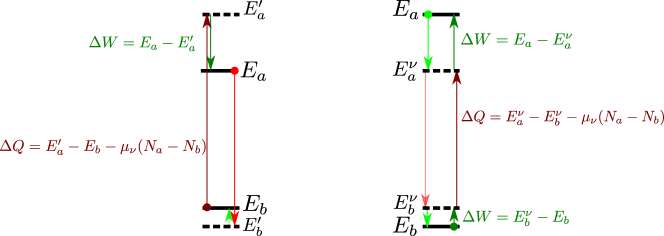
Another striking difference is that for state-conditioned feedback the heat transferred to and from the reservoir may differ for forward and backward transitions, whereas for jump-conditioned feedback it is the same (up to a sign).
To simulate merely the dynamics of the system, it is sufficient to replace the rates by their feedback-controlled versions in (1), (10), and (11). To track the dynamics of heat and entropy, it is necessary to generalize the thermodynamic laws (5) and (9) to instantaneous and piecewise-constant feedback:
For state-conditioned feedback, we can in analogy to (4) write for the energy currents and the feedback work current
| (12) |
where we have used that every control operation is tied to a change in states, such that the corresponding energy difference is multiplied with the corresponding transition probability. The total energy change (first law of thermodynamics) is then obtained by summing
| (13) |
which reflects the fact that the system is switching between energies , see Fig. 1. For jump-conditioned feedback, we proceed similarly any write (4) as
| (14) |
and their sum yields the same result as before. So far, these partitions into heat and feedback work contributions are somewhat arbitrary, they can be fixed using some microscopic intuition as we do in Secs. 0.2.1 and 0.2.2.
Even when the feedback does not change the system energies (e.g., when only the transition rates are modified), the local detailed balance relation (2) will no longer hold. To account for this and the proper corresponding energetic exchanges with the reservoirs, we parametrize the deviation from local detailed balance as esposito2012a
| (15) |
where is the true heat exchange associated with the transition and is a dimensionless feedback parameter 999 Note that one has the relation .. The feedback-free situation is thus reproduced for and .
With this, the last two lines of the system entropy balance (0.1.2) change into
| (16) |
As before, the first term is positive by construction and is identified with the entropy production rate of the (model) universe, the second term is still interpreted as the entropy production in the reservoirs (which are untouched by the feedback discussed here), but the last term quantifies how the feedback changes the entropy balance of the system and can thus be identified with an information current
| (17) |
such that the second law (9) generalizes to
| (18) |
Even at steady state (where ), it is now possible to have negative entropy produced in the reservoirs () as long as the information current counter-balances it such that the above modified second law (18) is still respected. Of course, this treatment neglects a (possibly large) part of the entropy produced in the unspecified feedback loop, it only takes into account its effect on the system. Maxwell demon feedbacks, in which we are mostly interested here, generate a situation where the feedback energy current is negligible , while at the same time, the information current is substantial . Both feedback schemes are capable of generating such scenarios.
0.1.5 Example: Maxwell-demon feedback for a two-level system
When we consider a two-level system with energies coupled to two (hot and cold) thermal reservoirs , the populations of its energy eigenstates follow in absence of feedback the rate equation
| (25) |
where by construction, we assume the implicit condition or . The rates satisfy local detailed balance (2) 101010Often occurring rates of this form are Bose distributions and or Fermi functions and , where the bare rates would cancel in (2).. To check thermodynamic consistency, consider the stationary energy current entering the system via the cold junction . This is always negative, which means that heat flows from hot to cold (Clausius formulation of the second law). This is also confirmed by looking at the entropy production rate (9), which at steady state (where and and the system contribution is negligible) simplifies to .
In presence of feedback, we now consider an increase or a decrease (compared to the feedback-free case) of the bare tunnelling rate to reservoir parametrized by feedback parameters and , such that the feedback-controlled rates relate to the feedback-free rates as
| (26) |
and we assume the energies to remain unperturbed , such that . This can significantly alter the transport characteristics 111111Consider the extreme limit , , , and , where the two-level system couples only to the cold reservoir when it is in its ground state and to the hot reservoir while it is in its excited state. In consequence, the energy can only flow from cold to hot reservoir.. Accordingly, we just replace in the rate matrix (25). Then, the stationary energy current entering the system from the cold junction becomes (for Maxwell-demon type feedbacks we have by energy conservation )
| (27) |
which is positive if and only if . Thus, with feedback we can direct the stationary energy current from the cold reservoir to the hot one by using sufficiently strong feedback parameters . The first law reads as before (Maxwell demon feedback by assumption does not inject energy), but the information current modifies the second law, such that the entropy production rate under feedback (18) becomes manifestly positive
0.2 Autonomous systems
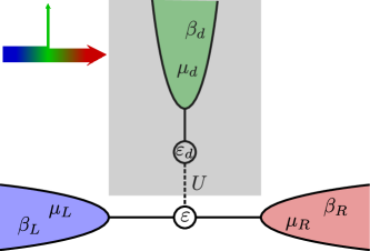
The implementation of external feedback control loops is experimentally challenging chida2017a and has shortcomings in its theoretical discussion (effective thermodynamic discussion, highly idealized assumptions on measurement and feedback speed, …). On-chip implementations of feedback loops in higher-dimensional rate equations do not suffer from these problems but allow for convenient cycle analyses mayrhofer2021a . Indeed, ideal Maxwell demons can – at least within the limits of perturbative descriptions – be very closely approximated sanchez2019b . Aiming at smallest systems, we focus here on setups that can direct the flow of energy from a cold reservoir towards a hot one by sacrificing a small fraction of the energy to a ultra-cold third terminal, see Fig. 2.
 |
 |
0.2.1 Autonomous four-level system: Interacting quantum dots
We first review a bipartite model shown in Fig. 2 left panel, that has been discussed theoretically with focus on battery charging strasberg2013a and also has been implemented experimentally koski2015a . It consists of two interacting two-level subsystems (quantum dots), such that our total system has four levels with the corresponding occupation probabilities of finding the first system in state while the second is in states , respectively. The first system is tunnel-coupled to two (left and right) reservoirs with additive transition rates, whereas the second is only coupled to one reservoir. Due to Coulomb interaction, the transition rates of one subsystem may depend on the state of the other. The rate matrix becomes
The rates can be written (beyond the wideband approximation) as products of bare tunneling rates and Fermi functions
| (28) |
where the left and right Fermi functions are given by and for the system reservoirs and analogously and for the demon reservoir.
Function: Cooling the left reservoir
To implement cooling on the left reservoir while and , one needs a cold demon reservoir and energies and chemical potentials tuned such that and , and furthermore some asymmetry in the left and right tunnelling rates, such that . A typical trajectory in this operational regime is depicted in Fig. 3.
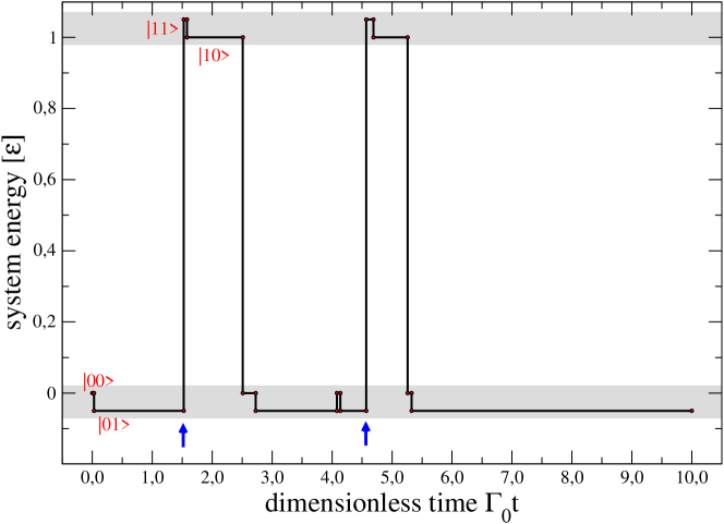
Since the device operates stochastically, one has unsuccessful loops like (which has zero net energy exchange), but in the chosen regime, successful loops like become likely. This loop effectively transfers energy out of the left reservoir to the demon reservoir with fraction and the right reservoir with fraction . Thus, the regime of a proper Maxwell demon is reached when we have while the directionality of all transitions is maintained. The required conditions on parameters and and can be simultaneously fulfilled strasberg2013a .
Relation to the feedback-controlled model
We can introduce the marginal probabilities for the state of the controlled system by summing over the states of the demon dot
| (29) |
and when constructing the differential equations for them we rewrite . The in reality time-dependent prefactor can in the limit of a very fast demon reservoir be replaced by a constant
| (30) | ||||
where and , to obtain a coarse-grained rate equation esposito2012b ; ehrich2021a ; strasberg2022 for the probabilities of the system dot being empty or filled like shown by the shaded regions of Fig. 3, respectively. In the limit where and , the coarse-grained rate matrix simplifies 121212 This happens at low demon reservoir temperatures with e.g. . It is also the limit where the measurement becomes perfect and system and demon dot are always anti-correlated. further into
| (33) |
In this, we see that the effective transition energy for the relaxation rate is different from the transition energy for the excitation, such that the autonomous four-level system effectively implements a state-conditioned feedback discussed in Sec. 0.1.4. The relevant ratios of effective transition rates for our entropic balance can be written as
| (34) |
where we have used that the heat transfer for an initially filled system dot (and empty demon dot) is , whereas it is for an initially empty system (and filled demon dot). From this, we can identify with (15) the energy differences and , which can be satisfied 131313 These shifts can be understood as unloading of the dot transfers energy to the left or right lead, wheras loading requires energy (the difference is transferred to the demon reservoir as effective feedback work). with energies , and and . The feedback parameters become
| (35) |
such that .
We can thus write for the coarse-grained energy currents
| (36) |
These currents match what is obtained from the microscopic four-level model in the limit of a fast and precise demon.
Accordingly, the information current becomes
| (37) |
As the coarse-grained entropy production under-estimates the full entropy production esposito2012b , and the coarse-grained energy currents converge to the ones from the microscopic model , it follows that the information current is smaller than the entropy production in the controller reservoir, such that the information gained in the measurement is only partially used in the feedback loop. Furthermore, it can be concluded that when we evaluate the thermodynamic uncertainty relation barato2015a , (where and are energy or matter current and its associated noise over an arbitrary junction), with the coarse-grained entropy production instead, we can find regimes where it is violated.
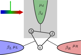
0.2.2 Autonomous three-level system
We now consider a three-level system as in Fig. 2 right panel, with its three transitions selectively driven by three independent reservoirs. Such a system could be the single-charged sector of a triple quantum dot (see e.g. Ref. seo2013a for an experimental implementation). We assume that the left (cold) reservoir drives the large transition between ground and second excited state, the right (hot) reservoir the smaller transition between ground and first excited state, and the demon reservoir (coldest) the remaining one between first and second excited state 141414 This is different from the commonly used quantum absorbtion refrigerator (QAR) levy2012b ; linden2010a : First, in a QAR the hot reservoir drives the large excitation above the ground state. Second, a QAR would require the transition between the two excited states driven by a work reservoir (e.g. a reservoir of substantially higher temperature than the hot and cold ones). Third, the operational regime of a QAR is characterized by a non-negligible energy current from the work reservoir , with the cofficient of performance limited by its Carnot value . Unlike a Maxwell demon, a QAR is thus energy-dominated, it could be implemented by reverting the temperature hierarchy to .. We consider here the limit of a low-temperature demon reservoir with negligible energetic contribution that reverses the usual heat flow. In the basis , the rate matrix for our model reads
| (41) |
where denotes the excitation and the de-excitation rate due to reservoir .
Function: Cooling the left reservoir
In the desired operational mode, the second excited state is occasionally reached from the ground state by the absorbtion of energy from the cold left reservoir (implementing cooling). The ultra-cold demon reservoir then takes a fraction of that energy to transfer the system from the second to its first excited state. Finally, the hot reservoir absorbs heat by allowing the transfer from the first excited state back to the ground state, closing the cycle. The opposite process is blocked by the ultra-cold demon reservoir in the intended regime, see Fig. 4 for a typical trajectory.
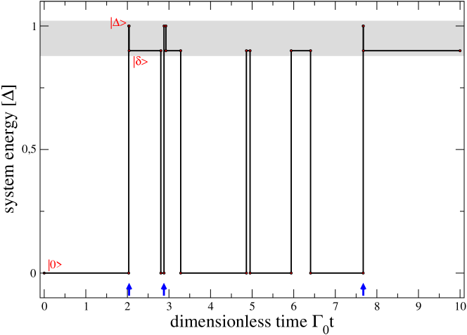
Thus, for a successful cycle , energy is taken from the left reservoir, while energies and are dissipated into the demon and right reservoirs, respectively. The Maxwell demon limit is thus approached when , while the directionality of transitions is maintained. For our model, this requires and .
The stationary currents entering the system from the reservoirs read
| (42) |
where . The other currents are tightly coupled and , such that the sum of all stationary currents vanishes (first law) and by using we can implement cooling of the cold left reservoir ().
At steady-state, the entropy production rate (9) thus reads
| (43) |
Thus, cooling occurrs when the prefactor in round brackets is positive, i.e., when . Furthermore, by choosing the energy dissipated into the demon reservoir can be made arbitrarily small while the entropy produced there remains large due to its low temperature . This already indicates a demon operational mode 151515 An efficiency of the device could be defined by , which is upper-bounded by unity as ., but we can make the relation to the external control loop more explicit by applying a similar coarse-graining procedure as before.
Relation to the feedback-controlled model
In the limit where the demon reservoir rates are both significantly larger than the others while maintaining local detailed balance (2) (consider e.g. , with Bose distribution in the limit ), we can formally coarse-grain (a similar argument is used in Sec. V of Ref. strasberg2014a ) the rate equation by introducing the probability to be in any of the excited states 161616Technically, we construct the equation for from the rate equation and rewrite and in all equations. as indicated by the shaded region in Fig. 4
| (44) |
Then, the coarse-graining approximation can be implemented by using that the conditional probabilities of being in one of the excited states are given by
such that the coarse-grained rate matrix for the states becomes
| (47) |
Since the ratios of the and already give the proper heat exchanges with those reservoirs, the three-level model thus effectively implements jump-conditioned feedback from Sec. 0.1.4. From (15) we can directly identify the feedback parameters as
| (48) |
such that . In the zero-temperature demon limit, the cold reservoir is thus associated with divergent (infinitely strong) feedback.
The stationary energy current from the left reservoir becomes
| (49) |
such that cooling is possible under the same conditions as before. The energy current from the hot reservoir is fixed by the tight coupling condition and also the energy current injected by the feedback becomes (as one may verify). These currents match what is obtained for the microscopic three-level model in the limit for the left, right, and controller reservoir, respectively.
Accordingly, the entropy produced in the demon reservoir is given by . This matches the effective information current resulting from the feedback, which becomes
| (50) |
The three-level implementation is thus more efficient than the four-level version not only by its reduced complexity, but also its more efficient use of information: The information current due to the demon precisely corresponds to the entropy produced in the feedback loop. The drawback is that there is no parameter to turn off the feedback smoothly (like was used in the four-level model).
Electronic implementation
One possibility to implement an electronic three-level system is in the Coulomb-blockade regime of two Coulomb-coupled quantum dots with effective single-particle onsite energies and . Preferentially, the left (cold) reservoir should load and unload a dot mode with charging energy , the right (hot) reservoir should load and unload a mode with charging energy . The selectivity of the coupling may be realized by using peaked reservoir spectral functions (which may be generated or enhanced further by connecting over additional fine-tuned quantum dots ehrlich2021a ) resonant with the corresponding transition energies and , respectively. The remaining transition between the two singly-charged modes is made possible by the action of a third (demon) reservoir, which leaves the particle number in the system constant 171717 Any capacitive interaction with coupling operator will trigger transitions between eigenmodes of the system ..
If one aims at setups where one has only energy but no particle exchange, one would need three particle-conserving reservoirs. Then, an electronic implementation of a three-level system would be possible using the singly charged sector of three tunnel-coupled quantum dots coupled to three particle-conserving reservoirs. An original interaction coupling to will then generate transition operators and energy renormalizations for all triple dot modes. Also here, the selectivity of the interaction could be implemented by tuning the reservoir parameters accordingly.
The rates for the demon reservoir in the double-dot case or all reservoirs in the singly-charged sector of the triple dot case can be microscopically calculated schaller2014 . To see that, consider a fermionic reservoir with a coupling of the form
| (51) |
where is a generic system coupling operator, and describes the reservoir-internal scattering 181818 A toy model for such a reservoir could be a chain with modes (where the actual reservoir limit is obtained for ) with homogeneous on-site energies and tunnelling amplitudes . For this, one can use the unitary transformation to diagonalize it exactly into with . When we couple this reservoir at its first site to a system via , we would obtain . and the term with the Fermi function has been introduced to cancel the expectation value of the coupling operator at equilibrium 191919Without renormalization, such an interaction would perturb the equilibrium state of the reservoir.. The correlation function can then be written as a two-fold integral , where we have introduced the function that describes the scattering processes inside the reservoir 202020 For the chain model reservoir it would for assume the form , which shows that by tuning and one may modify the spectral function of the reservoir.. Independent of the chemical potential (which may be used to tune the overall magnitude), the Fourier transform obeys the KMS relation , which implies that the associated rates obey the detailed balance condition (2) with and . In order to have not too small rates, the actual chemical potential should be tuned near the desired transition energy. Furthermore, energetic filtering for the chain toy model is possible by choosing also resonant with the desired transition energy and small . Further simplifications are possible when the scattering function is approximately constant 212121When , we obtain with Bose distribution , leading to a transition rate . .
Unfortunately, particularly in the interesting Maxwell demon limit where one has two near-degenerate excitation energies in the system, and energetic filtering alone is insufficient. In this case, one can additionally tune the system and reservoir couplings to maintain the selectivity of the reservoirs 222222 For a homogeneous triple quantum dot one finds with , a representation in terms of two degenerate eigenmodes . Then, (up to dephasing terms ) the capacitive coupling drives transitions between states , drives transitions between (desired) and (can be filtered), and finally drives all possible transitions (but and can be filtered). This can be further improved when non-homogeneous tripledot systems are considered. .
0.3 Conclusions
To answer the main question: Maxwell’s demon, incarnated by autonomous demonic refrigerators, can be be pretty small (our considerations suggested three levels). In addition, it does not require a bipartite system-controller setup and can also be very efficient in the sense that the entropy produced in the feedback loop is equivalent to the information current entering the effective controlled system.
The present contribution has focused on the mathematical framework of rate equations with the associated limitations. Generalizations to equations describing situations of near-degenerate energies trushechkin2021a , with system-reservoir correlations beyer2019a , and the strong-coupling regime strasberg2018a in autonomous systems or not perfectly-energetic measurements schaller2018a ; seah2020a and delay effects debiossac2020a in external loops are interesting pathways of further research.
Acknowledgements.
The author thanks C. Kohlfürst and P. Strasberg for helpful comments on the manuscript and for generous conference support by the CRC 1242 (Project ID No. 278162697).References
- [1] A. C. Barato and U. Seifert. Thermodynamic uncertainty relation for biomolecular processes. Physical Review Letters, 114:158101, 04 2015.
- [2] J. Bergli, Y. M. Galperin, and N. B. Kopnin. Information flow and optimal protocol for a Maxwell-demon single-electron pump. Physical Review E, 88:062139, Dec 2013.
- [3] K. Beyer, K. Luoma, and W. T. Strunz. Steering heat engines: A truly quantum Maxwell demon. Phys. Rev. Lett., 123:250606, Dec 2019.
- [4] H.-P. Breuer and F. Petruccione. The Theory of Open Quantum Systems. Oxford University Press, Oxford, 2002.
- [5] K. Chida, S. Desai, K. Nishiguchi, and A. Fujiwara. Power generator driven by Maxwell’s demon. Nature Communications, 8:15310, 2017.
- [6] S. Ciliberto. Autonomous out-of-equilibrium Maxwell’s demon for controlling the energy fluxes produced by thermal fluctuations. Phys. Rev. E, 102:050103, Nov 2020.
- [7] N. Cottet, S. Jezouin, L. Bretheau, P. Campagne-Ibarcq, Q. Ficheux, J. Anders, A. Aufféves, R. Azouit, P. Rouchond, and B. Huard. Observing a quantum Maxwell demon at work. Proceedings of the National Academy of Sciences of the United States of America, 114:7561, 2017.
- [8] M. Debiossac, D. Grass, J. J. Alonso, E. Lutz, and N. Kiesel. Thermodynamics of continuous non-Markovian feedback control. Nature Communications, 11:1360, 2020.
- [9] J. Ehrich. Tightest bound on hidden entropy production from partially observed dynamics. Journal of Statistical Mechanics: Theory and Experiment, 2021(8):083214, aug 2021.
- [10] J. Ehrich and D. A. Sivak. Energy and information flows in autonomous systems. Frontiers in Physics, 11:1108357, 2023.
- [11] J. Ehrich, S. Still, and D. A. Sivak. Energetic cost of feedback control. Phys. Rev. Res., 5:023080, May 2023.
- [12] T. Ehrlich and G. Schaller. Broadband frequency filters with quantum dot chains. Phys. Rev. B, 104:045424, Jul 2021.
- [13] C. Emary. Delayed feedback control in quantum transport. Philosophical Transactions of the Royal Society A, 371:1471, 2013.
- [14] M. Esposito. Stochastic thermodynamics under coarse graining. Physical Review E, 85:041125, Apr 2012.
- [15] M. Esposito, U. Harbola, and S. Mukamel. Entropy fluctuation theorems in driven open systems: Application to electron counting statistics. Physical Review E, 76(3):031132, 2007.
- [16] M. Esposito and G. Schaller. Stochastic thermodynamics for ”Maxwell demon” feedbacks. Europhysics Letters, 99:30003, 2012.
- [17] N. Freitas and M. Esposito. Characterizing autonomous Maxwell demons. Phys. Rev. E, 103:032118, Mar 2021.
- [18] J. M. Horowitz and M. Esposito. Thermodynamics with continuous information flow. Physical Review X, 4:031015, Jul 2014.
- [19] J. V. Koski, A. Kutvonen, I. M. Khaymovich, T. Ala-Nissila, and J. P. Pekola. On-chip Maxwell’s demon as an information-powered refrigerator. Physical Review Letters, 115:260602, Dec 2015.
- [20] H. Leff and A. Rex. Maxwell’s demon: entropy, information, computing. Princeton University Press, Princeton, New Jersey, 1990.
- [21] H. Leff and A. Rex. Maxwell’s demon 2: Entropy, Classical and Quantum Information, Computing. CRC Press, Bristol, 2002.
- [22] A. Levy and R. Kosloff. Quantum absorption refrigerator. Phys. Rev. Lett., 108:070604, Feb 2012.
- [23] N. Linden, S. Popescu, and P. Skrzypczyk. How small can thermal machines be? The smallest possible refrigerator. Physical Review Letters, 105(13):130401, 2010.
- [24] D. Mandal, H. T. Quan, and C. Jarzynski. Maxwell’s refrigerator: An exactly solvable model. Phys. Rev. Lett., 111:030602, Jul 2013.
- [25] K. Maruyama, F. Nori, and V. Vedral. Colloquium: The physics of Maxwell’s demon and information. Rev. Mod. Phys., 81(1):1–23, 2009.
- [26] J. C. Maxwell. Theory of Heat. Longmans, Greens, and Co., London, 1871.
- [27] R. D. Mayrhofer, C. Elouard, J. Splettstoesser, and A. N. Jordan. Stochastic thermodynamic cycles of a mesoscopic thermoelectric engine. Phys. Rev. B, 103:075404, Feb 2021.
- [28] R. Sánchez, P. Samuelsson, and P. P. Potts. Autonomous conversion of information to work in quantum dots. Phys. Rev. Res., 1:033066, Oct 2019.
- [29] R. Sánchez, J. Splettstoesser, and R. S. Whitney. Nonequilibrium system as a demon. Phys. Rev. Lett., 123:216801, Nov 2019.
- [30] G. Schaller. Open Quantum Systems Far from Equilibrium, volume 881 of Lecture Notes in Physics. Springer, Cham, 2014.
- [31] G. Schaller, J. Cerrillo, G. Engelhardt, and P. Strasberg. Electronic Maxwell demon in the coherent strong-coupling regime. Phys. Rev. B, 97:195104, May 2018.
- [32] S. Seah, S. Nimmrichter, and V. Scarani. Maxwell’s lesser demon: A quantum engine driven by pointer measurements. Phys. Rev. Lett., 124:100603, Mar 2020.
- [33] U. Seifert. Stochastic thermodynamics, fluctuation theorems and molecular machines. Reports on Progress in Physics, 75:126001, 2012.
- [34] M. Seo, H. K. Choi, S.-Y. Lee, N. Kim, Y. Chung, H.-S. Sim, V. Umansky, and D. Mahalu. Charge frustration in a triangular triple quantum dot. Phys. Rev. Lett., 110:046803, Jan 2013.
- [35] P. Strasberg. Quantum Stochastic Thermodynamics. Oxford University Press, Oxford, 2022.
- [36] P. Strasberg, G. Schaller, T. Brandes, and M. Esposito. Thermodynamics of a physical model implementing a Maxwell demon. Physical Review Letters, 110:040601, 2013.
- [37] P. Strasberg, G. Schaller, T. Brandes, and C. Jarzynski. Second laws for an information driven current through a spin valve. Physical Review E, 90:062107, Dec 2014.
- [38] P. Strasberg, G. Schaller, T. L. Schmidt, and M. Esposito. Fermionic reaction coordinates and their application to an autonomous Maxwell demon in the strong-coupling regime. Phys. Rev. B, 97:205405, May 2018.
- [39] A. Trushechkin. Unified Gorini-Kossakowski-Lindblad-Sudarshan quantum master equation beyond the secular approximation. Phys. Rev. A, 103:062226, Jun 2021.
- [40] M. D. Vidrighin, O. Dahlsten, M. Barbieri, M. S. Kim, V. Vedral, and I. A. Walmsley. Photonic Maxwell’s demon. Physical Review Letters, 116:050401, Feb 2016.