Understanding correlations in BaZrO3: Structure and dynamics on the nano-scale

Abstract

Barium zirconate BaZrO3 is one of few perovskites that is claimed to retain an average cubic structure down to 0 at ambient pressure, while being energetically very close to a tetragonal phase obtained by condensation of a soft phonon mode at the R-point. Previous studies suggest, however, that the local structure of BaZrO3 may change at low temperature forming nanodomains or a glass-like phase. Here, we investigate the global and local structure of BaZrO3 as a function of temperature and pressure via molecular dynamics simulations using a machine-learned potential with near density functional theory (DFT) accuracy. We show that the softening of the octahedral tilt mode at the R-point gives rise to weak diffuse superlattice reflections at low temperatures and ambient pressure, which are also observed experimentally. However, we do not observe any static nanodomains but rather soft dynamic fluctuations of the ZrO6 octahedra with a correlation length of 2 to 3 over time-scales of about 1. This soft dynamic behaviour is the precursor of a phase transition and explains the emergence of weak superlattice peaks in measurements. On the other hand, when increasing the pressure at 300 we find a phase transition from the cubic to the tetragonal phase at around 16, also in agreement with experimental studies.

I Introduction

Perovskite oxides constitute a prominent class of materials with a wide range of different properties, such as ferroelectricity, colossal magnetoresistance, electronic and/or ionic conductivity, piezoelectricity, superconductivity, metal-insulator transition, luminescence, and many more [1].

The prototypical oxide perovskite structure is cubic, with the general chemical formula ABO3, where the A and B sites can accommodate a wide variety of elements from the periodic table. Many perovskites are cubic at high temperatures but upon cooling most undergo one or several structural phase transitions, which depend sensitively on the choice of A and B. These phase transitions are often related to tilting of the BO6 octahedra, typically referred to as antiferrodistortive transitions. Commonly they are out-of-phase and in-phase tilting phonon modes related to instabilities at the R and/or M-points of the Brillouin zone.

Barium zirconate BaZrO3 is rather unique among the oxide perovskites. Neutron powder diffraction studies show that BaZrO3 at ambient pressure maintains its high temperature cubic structure down to temperatures close to zero Kelvin [2, 3, 4]. While the antiferrodistortive R-tilt mode softens substantially with decreasing temperature, its frequency remains positive as the temperature approaches zero Kelvin [5, 6].

While the latter experiments have clearly established the long-range order, the short-range order of the cubic BaZrO3 phase is more controversial. Raman spectra show pronounced peaks despite that first-order scattering is prohibited by symmetry reasons for cubic systems [7, 8, 9]. This has been interpreted as evidence for distorted nanodomains with lower than cubic symmetry, giving rise to first-order broad Raman spectra [7, 10]. A somewhat similar idea, an “inherent dynamical disorder”, has been put forward to account for the apparent local deviation from the cubic structure identified by Raman spectroscopy [9]. On the other hand, Raman studies of BaZrO3 single crystals associated these spectral features to second-order events, but stated that it is likely that the overall scattering intensity finds its origin in some other type of local disorder [11]. It has also been argued that a structural “glass state” may be formed upon cooling due to the extremely small energy differences between the phases allowed from condensation of the R mode [12]. The structural order could then be distorted on the local scale but appear cubic in diffraction experiments.

Recent electron diffraction experiments by Levin et al. [13] suggest that BaZrO3 undergoes a local structural change associated with correlated out-of-phase tilting of the ZrO6 octahedra when the temperature is reduced below 80. They found weak, but clear, diffuse scattering intensity at the R-point $(3/2,1/2,1/2)$, where the soft mode connecting the cubic to the tetragonal phase is located; yet their average structure remained cubic. The authors suggested that nanometer-sized domains (“nanodomains”) with local tetragonal structure could explain the diffraction results. The size of these domains was estimated to be about 2 to 3nm based on the full width half maximum (FWHM) of the diffraction peaks. They stated that the emergence of these relatively sharp superlattice reflections resembles a phase transition more than dynamic correlations, but their measurements could not conclusively discern between static and dynamic effects.

The pressure dependence of BaZrO3 at room temperature has been investigated by several authors [14, 7, 15, 16]. In a recent combined X-ray diffraction and Raman spectroscopy study [16], it was found that BaZrO3 undergoes a single phase transition around 10 from the cubic ($Pm\overline{3}m$) to the tetragonal ($I4/mcm$) phase and retains that structure up to 45.1. No second phase transition to an orthorhombic or any other tilted phase was observed. This confirms a previous high pressure X-ray diffraction study from 0 to 46.4 [14], where also a single transition from the cubic to the tetragonal phase was obtained, but at the considerably higher pressure of 17.2. However, a recent study based on Raman spectroscopy [15] found two structural phase transitions, the first from the cubic to a rhombohedral ($R\overline{3}c$) phase at 8.4 and the second from the rhombohedral to the tetragonal phase at 11.

Here, we construct a machine-learned potential using the neuroevolution potential (NEP) approach trained with density functional theory (DFT) data to be able to simulate the system over long time-scales (100ns) using large systems (15 million atoms) with near DFT accuracy. The phase diagram for BaZrO3 is mapped out as a function of temperature and pressure and compared with experiments. The static and dynamic structure factors as a function of wavevector and frequency are computed and their dependence on temperature and pressure are investigated. Detailed and direct comparison is made with the electron diffraction data by Levin et al. [13] and the dynamics close to the R-point is clarified. Finally, the spatial and temporal correlations of the local tilt angles for each individual ZrO6 octahedron are computed to elucidate the three-dimensional structure and dynamics of BaZrO3 as a function of temperature and pressure.

II Results

II.1 Instabilities and phase diagram

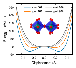
Figure 1: The potential energy landscape for the R-tilt mode obtained with the NEP model as function of the oxygen atom displacement. The inset shows the atoms in a tilted structure, where red is oxygen, green zirconium and the blue faces show the ZrO6 octahedra.

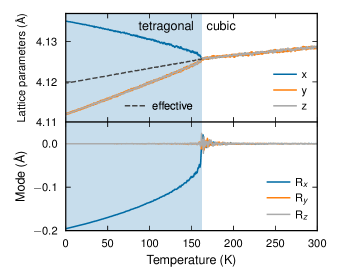
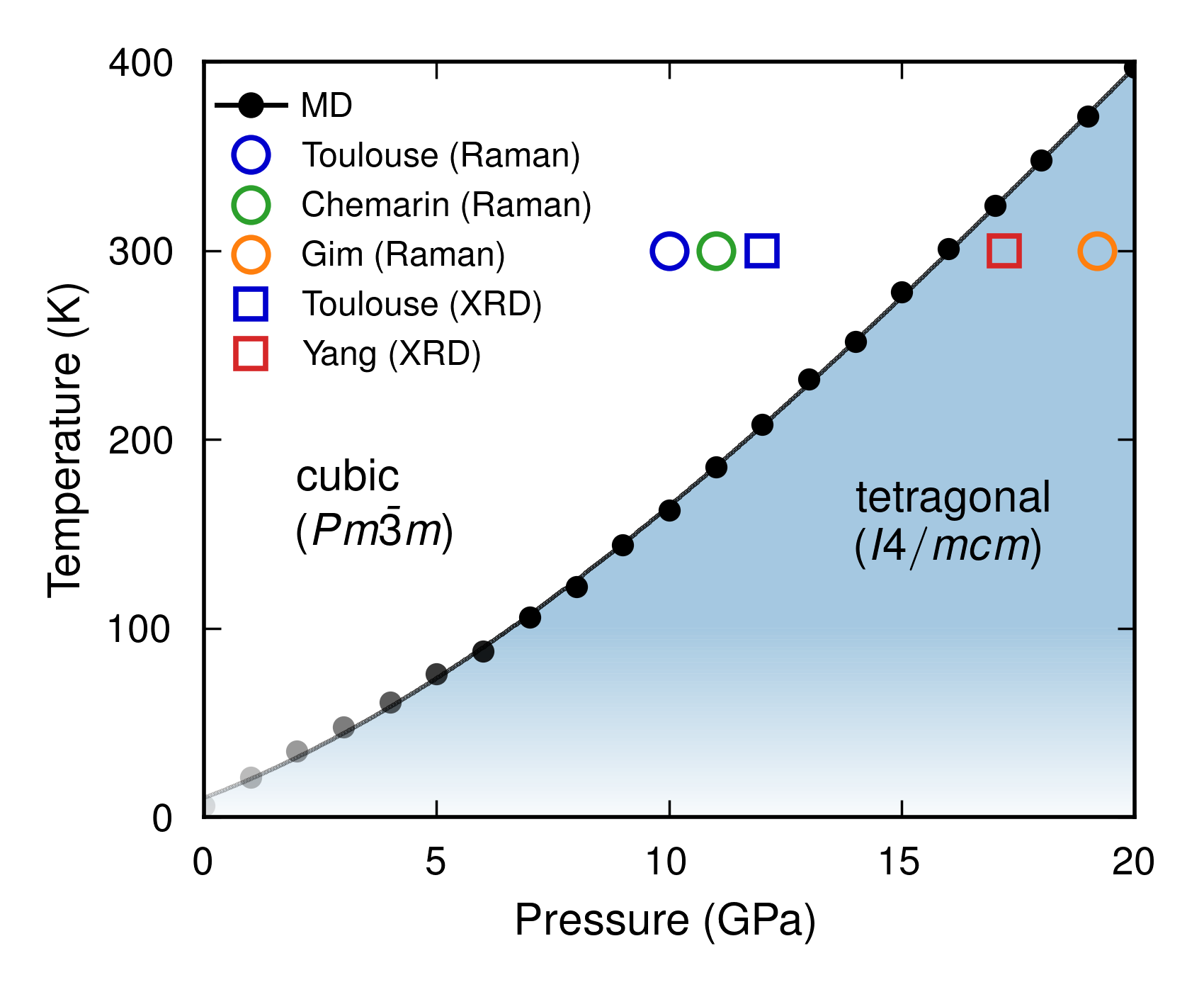
Figure 2: a) Temperature dependence of lattice parameters and R-mode coordinates at 10 from a cooling MD run in the NPT ensemble. The phase transition from the cubic to the tetragonal phase is observed at about 160. The effective lattice parameter for the tetragonal phase is given by $V^{1/3}$, where $V$ is the volume per formula unit. b) Phase diagram from cooling MD runs. Here, the region below 100 is shown with increasing transparency to reflect the uncertainty due to the classical sampling in MD. Experimental Raman spectroscopy data from Refs. 7, 16, 15 and XRD data from Refs. 14, 16.

DFT calculations based on the CX functional yield a lattice parameter for cubic BaZrO3 of 4.20, for which the phonon dispersion curves show only a very weak instability at the R-point [4]. When decreasing the lattice parameter the instability at the R-point increases and for 4.00 the dispersion curves also show an instability at the M-point (LABEL:sfig:dispersion).

In Fig. 1 we show the static energy landscape along the R-tilt mode as function of the oxygen atom displacement. For 4.00 a clear double well energy landscape is obtained with depths equal to -29.8 and located at +-0.25. This corresponds to a tilt angle of 7.1. We note that the M-mode instability for 4.00 is barely visible on the same energy scale (LABEL:sfig:mode_potential).

Next, we consider the system at finite temperatures and pressures. MD simulations are carried out in the NPT ensemble where the length of the cell vectors are allowed to fluctuate but the angles between them are kept fixed at 90. The system is cooled at constant pressure from high temperature at a rate of 40, which is sufficiently slow to avoid any noticeable hysteresis. We also note that it is due to the second-order nature of the phase transition that we can sample and observe it directly in MD simulations.

To monitor the dynamic evolution of the system we use the temperature dependence of the lattice parameters $a_{i}$ and the phonon mode coordinates $Q_{\lambda}$. The latter are obtained by phonon mode projections [17, 18]. The atomic displacements at each time are scaled back to the original cubic supercell and these scaled displacements $\boldsymbol{u}(t)$ are then projected on a tilt phonon mode $\lambda$ according to

$$Q_{\lambda}(t)=\boldsymbol{u}(t)\cdot\boldsymbol{e}_{\lambda}\ ,$$ (1)

where $\boldsymbol{e}_{\lambda}$ is the supercell eigenvector for mode $\lambda$. The mode eigenvectors are obtained using phonopy [19] and symmetrized such that each of the three degenerate modes corresponds to tilting around $x$, $y$, and $z$ directions, respectively. A gliding time average with width 20 is applied along the trajectory of the cooling simulation allowing us to extract the lattice parameters as well as the phonon mode coordinates $Q_{\lambda}$ as a practically continuous function of temperature.

In Fig. 2a the temperature dependence of the lattice parameters and R-mode coordinates are shown at 10 when the system is cooled from 300. At around 160 the lattice parameter in the $x$ direction deviates from the other two forming a tetragonal structure at the same time as the R_x mode condensates. This indicates a phase transition from the cubic $a^{0}a^{0}a^{0}$ ($Pm\bar{3}m$) to the tetragonal $a^{0}a^{0}c^{-}$ ($I4/mcm$) phase.

Cooling runs are repeated for various pressures and the resulting phase diagram is determined and shown in Fig. 2b. At 300 we find a phase transition to the tetragonal phase at 16.2. We do not see any condensation of the M-tilt modes (in-phase tilting) at any pressure or temperature. Furthermore, the phase transition only occurs to the tetragonal phase ($I4/mcm$), not to any orthorhombic or rhombohedral phases, except for a small region below 20 and around 4 to 5, where the rhombohedral ($R\overline{3}c$) structure becomes stable. However, for these low temperatures quantum fluctuations become important and we expect these to stabilize the tetragonal structure as discussed below. The observed lattice parameters as a function of temperature and pressure is shown in LABEL:sfig:lattice_parameters, and agrees well with experimental work [20].

Below about 100 quantum effects have been shown to be important to correctly model the stability of the cubic phase [6]. Therefore, the phase diagram obtained here using classical MD simulations becomes less accurate at low temperatures. This is indicated in Fig. 2 by the increased transparency of the color at low temperatures. We note here that while the classical MD simulations predict that the system becomes tetragonal at zero temperature and pressure, it is likely not the case if quantum fluctuations are included (see LABEL:sfig:Rmode_frequency and Ref. 6).

The phase transition to the tetragonal phase as function of pressure has been investigated experimentally by Raman spectroscopy [7, 16, 15] and XRD measurements [14, 16]. The experimental results are rather scattered. In Raman studies the phase transition to the tetragonal structure was observed at 11 [7], 10 [16], and 19.2 [15] at room temperature, and in XRD measurements at 17.2 [14] and 12 [16]. Our observed phase transition, from the cubic to the tetragonal phase, at 16.2 falls approximately in the middle of experimentally observed range. In Ref. 15 a transition to a rhombohedral ($R\overline{3}c$) structure was also obtained at 8.4. This type of transition was, however, neither observed in the other experimental studies nor does it appear in the present simulations.

II.2 The structure factor: Temperature dependence

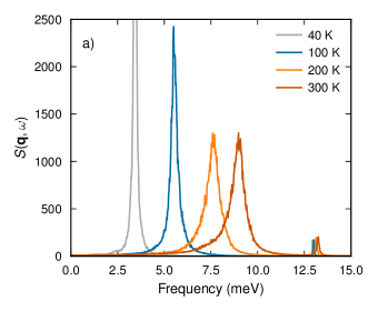
Figure 3: Dynamical structure factor, $S(\boldsymbol{q},\omega)$, for various temperatures at 0. Here, $\boldsymbol{q}=\frac{2\pi}{a}(3/2,1/2,1/2)$, corresponding to the R-point in the second Brillouin zone.

Next, we consider the temperature dependence of the structure factor at ambient (zero) pressure. The intermediate scattering function is defined as

$$F(\boldsymbol{q},t)=\frac{1}{N}\left<\sum_{i}^{N}\sum_{j}^{N}\mathrm{exp}\left[i\boldsymbol{q}\cdot(\boldsymbol{r}_{i}(t)-\boldsymbol{r}_{j}(0))\right]\right>\ ,$$ (2)

where $\boldsymbol{r}_{i}(t)$ denotes the position of atom $i$ at time $t$, $N$ is the number of atoms, and $\left<\ldots\right>$ indicates a time average. The dynamic structure factor $S(\boldsymbol{q},\omega)$ is obtained by a temporal Fourier transform of $F(\boldsymbol{q},t)$.

We calculate the intermediate scattering function $F(\boldsymbol{q},t)$ from MD simulations in the NVE ensemble. The total simulation time for a run is 1 and $F(\boldsymbol{q},t)$ is averaged over $100$ independent such simulations. The corresponding dynamic structure factor $S(\boldsymbol{q},\omega)$ is shown in Fig. 3 at the R-point $\boldsymbol{q}=\frac{2\pi}{a}(3/2,1/2,1/2)$.

The lower peaks, below 10, correspond to the R tilt-mode and the peaks around 13 correspond to the acoustic mode. The R tilt-mode shows a strong temperature dependence, softening with decreasing temperature. This is in good agreement with previous experimental and theoretical modeling [6, 5].

Next, we consider the static structure factor $S(\boldsymbol{q})$, which is related to the intermediate scattering function and the dynamic structure factor via

$$S(\boldsymbol{q})=F(\boldsymbol{q},t=0)=\frac{1}{2\pi}\int_{-\infty}^{\infty}S(\boldsymbol{q},\omega)\mathrm{d}\omega.$$ (3)

The partial static structure factors $S_{\alpha\beta}(\boldsymbol{q})$ are then evaluated as

$$S_{\alpha\beta}(\boldsymbol{q})=\frac{1}{N}\left<\sum_{i\in\alpha}^{N_{\alpha}}\sum_{j\in\beta}^{N_{\beta}}\exp{\left[i\boldsymbol{q}\cdot(\boldsymbol{r}_{i}(t)-\boldsymbol{r}_{j}(t))\right]}\right>,$$ (4)

where $\alpha$ and $\beta$ denote the atom types ($\alpha$ = Ba, Zr or O), the summation runs over all atoms of the given type and $N_{\alpha}$ is the number of atoms of type $\alpha$. The static structure factor is calculated from MD simulations in the NVT ensemble at 0 and different temperatures. For each temperature, we average over 40 independent simulations that are each 100 long.

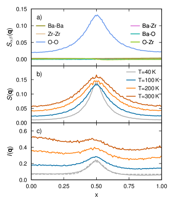
Figure 4: Structure factors calculated from MD simulations at 0. Here, $\boldsymbol{q}=\frac{2\pi}{a}(3/2,1/2,x)$, which corresponds to a horizontal 1D slice of the data given in Fig. 5, i.e., starting from an M-point ($x=0$), passing an R-point ($x=1/2$), and ending at another M-point ($x=1$). a) Partial structure factors $S_{\alpha\beta}(\boldsymbol{q})$ at 100. b) Total structure factor $S(\boldsymbol{q})$ at 40, 100, 200 and 300. c) Scattering intensity $I(\boldsymbol{q})$ at 40, 100, 200 and 300. The dashed line for 40 shows a Gaussian fit.

We consider first the partial static structure factors $S_{\alpha\beta}$ at 100 calculated along the Brillouin zone path $\boldsymbol{q}=\frac{2\pi}{a}(3/2,1/2,x)$ with $x:0\to 1$, shown in Fig. 4a, corresponding to a path $M\to R\to M$ also used by Levin et al. [13] (see their Fig. 5). The oxygen-oxygen part gives rise to large intensity at the R-point ($x=1/2$), in agreement with the soft oxygen tilt mode at R, as well as a background intensity. The other partial static structure factors only give rise to a very weak background intensity.

The temperature dependence of the static structure factor $S(\boldsymbol{q})$ is shown in Fig. 4b at 40, 100, 200, and 300. For all temperatures there is a peak at the R-point ($x$=1/2). To further understand this, consider the static structure factor for a harmonic system [21] in the classical limit

$$S(\boldsymbol{q})\propto\sum_{\lambda}^{N_{\text{modes}}}|F^{\text{ph}}_{\lambda}(\boldsymbol{q})|^{2}\frac{2k_{\text{B}}T}{(\hbar\omega_{\lambda})^{2}}\ ,$$ (5)

where the sum runs over all phonon modes for the given $\boldsymbol{q}$-point and $F^{\text{ph}}_{\lambda}(\boldsymbol{q})$ is the phonon structure factor containing the Debye-Waller factor and mode selection rules [22]. Therefore, we roughly expect the intensity to increase linearly with temperature $T$ and to scale with frequency as $1/\omega^{2}$. The peak height of $S(\boldsymbol{q})$ is almost constant with temperature whereas the background increases linearly with temperature in accordance with a harmonic system. The constant peak height is due to that the tilt-frequency of the R-mode softens from 9 to about 3 between 300 and 40, since $300/9^{2}\approx 40/3^{2}$. Thus, the structure factor at the R-point remains more or less constant with temperature. The clear peak at 40 is therefore a result of the tilt-frequency of the R-mode softening with temperature.

The present MD simulations are based on classical mechanics. Quantum fluctuations of the atomic motion start to become important for the R-mode frequency below 100 [6]. We have tested the effect quantum fluctuations on the above peak height using a self-consistent phonon approach (see LABEL:sfig:Sq_harmonic). The peak height at the R-point is slightly reduced by including the quantum effects, but a clear peak at 40 is still present.

Lastly, to get a one-to-one comparison with the electron beam diffraction experiments carried out by Levin et al. [13], we determine the intensity, $I(\boldsymbol{q})$, by weighting the partial structure factors with their corresponding electron atomic scattering factors according to

$$I(\boldsymbol{q})=\sum_{\alpha}\sum_{\beta}f_{\alpha}(q)f_{\beta}(q)S_{\alpha\beta}(\boldsymbol{q})\ .$$ (6)

Here, $f_{\alpha}(q)$ are the $q$-dependent electronic scattering factors for the ions Ba^2+, Zr^4+, and O^2-, with numerical data taken from Ref. 23 (see LABEL:sfig:scattering_factors). The scattering factors are roughly proportional to the atomic number, reducing the oxygen contribution significantly. The peak at the R-point for the intensity $I(\boldsymbol{q})$ is reduced in height (relative to the background) (Fig. 4c) and there is barely any visible peak above 100. This is in good agreement with the observation by Levin et al. [13] that a weak and diffuse, yet discrete spot appears at the R-point below about 80. For 40 we also carry out a Gaussian fit of $I(\boldsymbol{q})$ with a constant background to extract the FWHM of 0.23, which is in very good agreement with the value of 0.22, reported by Levin et al. [13].

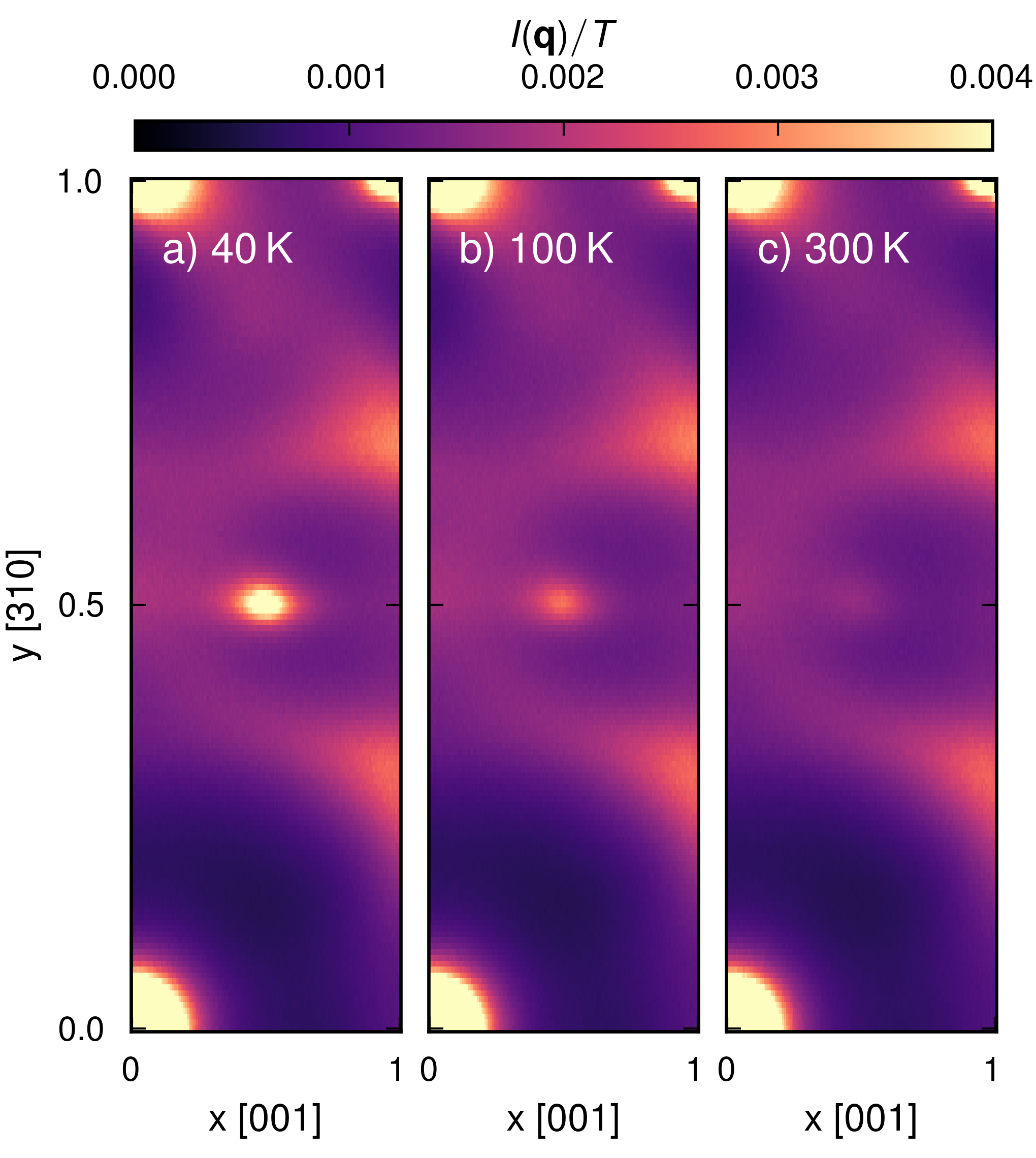
Figure 5: Intensity normalized by temperature, $I(\boldsymbol{q})/T$, calculated from MD simulations at a) 40, b) 100, and c) 300. Here, $\boldsymbol{q}=\frac{2\pi}{a}(3y,y,x)$. The lower left corner thus corresponds to the $\boldsymbol{q}$-point $\boldsymbol{q}=(0,0,0)$, the upper left corner to $\boldsymbol{q}=\frac{2\pi}{a}(3,1,0)$, the lower right corner to $\boldsymbol{q}=\frac{2\pi}{a}(0,0,1)$, and the upper right corner to $\boldsymbol{q}=\frac{2\pi}{a}(3,1,1)$. The center of the heatmaps corresponds to the R-point $\boldsymbol{q}=\frac{2\pi}{a}(3/2,1/2,1/2)$. Note also that the color scale is set such that diffuse scattering is visible, but in practice the intensity at the $\Gamma$-points are orders of magnitude larger.

Next, we extend the calculation of the intensity $I(\boldsymbol{q})$ to the same 2D space of $\boldsymbol{q}$-points as highlighted by Levin et al. [13] in their Figure 4. Because the intensity increases almost linearly with temperature (Eq. (5)), we plot $I(\boldsymbol{q})/T$ to enable easier comparison between temperatures. These normalized intensities are shown as heatmaps in Fig. 5. Heatmaps for the partial intensities $I_{\alpha\beta}(\boldsymbol{q})$ at 100 can be found in LABEL:sfig:partial_heatmaps. Most of the intensity heatmaps in Fig. 5 look very similar for all three temperatures. The larger intensities in the corners ($\Gamma$ points) corresponds to the Bragg peaks. The intensity between Bragg peaks, the diffuse scattering, arises due to thermal motion. The only real notable difference between the temperatures is the increased intensity in the middle of the heatmap (at the R-point $\boldsymbol{q}=\frac{2\pi}{a}(3/2,1/2,1/2)$) for lower temperatures. At 300 there is almost no peak visible at the R-point compared to the intensity level for the surrounding $\boldsymbol{q}$-points, whereas for 40 there is a very clear peak (as also seen in Fig. 4c). The notable intensities at $x$=1, $y$=1/3 and $x$=1, $y$=2/3 arise from the low frequency Ba and Zr modes between $\Gamma$ and M (and close to X) in the phonon dispersion ($\it cf.$ LABEL:sfig:dispersion_along_311 and LABEL:sfig:partial_heatmaps).

II.3 Tilt angle correlations: Temperature dependence

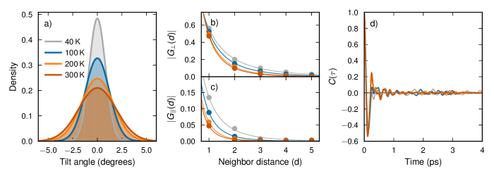
Figure 6: Distributions of the tilt angle $\theta^{\alpha}$ and its correlations from MD simulations at 0 and different temperatures. a) Tilt angle distribution, averaged over $\alpha=x,y,z$. Solid lines represent Gaussian fits with zero mean. b,c) Static tilt-angle correlation functions $G_{\parallel}(d)$ and $G_{\perp}(d)$ as a function of neighbor distance $d$. Solid lines are guides to the eye. d) Dynamic tilt-angle correlation function $C(\tau)$ as defined in Eq. (7) and averaged over $\alpha=x,y,z$.

To obtain a more local picture we now consider the tilt angle of each individual ZrO6 octahedron, and its static and dynamic correlations. We first extract the Euler angles for each octahedron from MD simulations. We employ the polyhedral template matching using ovito [24] as done in Ref. 25. This allows us to extract tilt angles around the $\alpha$ axis ($\alpha=x,y,z$) for an octahedron located at $(n_{x},n_{y},n_{z})$ at time $t$, $\theta^{\alpha}(n_{x},n_{y},n_{z},t)$. Here, we follow a similar notation as in Refs. 26, 27.

The distribution $P(\theta)$ over $\theta^{\alpha}(n_{x},n_{y},n_{z},t)$ averaged over $\alpha$, $(n_{x},n_{y},n_{z})$, and $t$ can now be determined (Fig. 6a). We notice that for all temperatures the distribution exhibits a Gaussian profile with zero mean and with a standard deviation that increases with temperature. The standard deviations are $\sigma=\qty{0.82}{}$, $\sigma=\qty{1.21}{}$, $\sigma=\qty{1.62}{}$, and $\sigma=\qty{1.90}{}$ for 40, 100, 200, and 300, respectively. In a classical harmonic system we expect the variance $\sigma^{2}$ to increase linearly with temperature but here, due to the softening of the R-tilt mode, the distribution over tilt angles shows a weaker temperature dependence.

Next, we consider the static tilt-angle correlation function between $\theta^{\alpha}(n_{x},n_{y},n_{z},t)$ and its neighboring octahedra. Here, we only consider neighbors along the [100], [010] and [001] directions. The static correlation function in the [100] direction is calculated as

$$G_{x}^{\alpha}(d)=\frac{\left<\theta^{\alpha}(n_{x}+d,n_{y},n_{z},t)\theta^{\alpha}(n_{x},n_{y},n_{z},t)\right>}{\left<\theta^{\alpha}(n_{x},n_{y},n_{z},t)\theta^{\alpha}(n_{x},n_{y},n_{z},t)\right>}\ ,$$

where $d$ corresponds to the number of neighbor distances between two octahedra in the $x$-direction and $\left<\ldots\right>$ denotes an average carried out over $(n_{x},n_{y},n_{z})$ and $t$. Similarly, one can define the static correlation function along the [010] direction, $G_{y}^{\alpha}(d)$, and along the [001] direction, $G_{z}^{\alpha}(d)$. In the cubic phase we only obtain two symmetrically distinct static correlation functions, $G_{\perp}(d)$ and $G_{\parallel}(d)$, corresponding to if the rotation axis (superscript $\alpha$) is perpendicular or parallel to the neighbor direction, respectively.

The result for the static tilt-angle correlation functions are shown in Fig. 6b. For both $G_{\perp}(d)$ and $G_{\parallel}(d)$ the correlation alternates between positive and negative values when increasing the neighbor distance, since the R-tilt mode dominates that motion [13, 26, 25]. We thus only show $|G_{\perp}(d)|$ and $|G_{\parallel}(d)|$ in Fig. 6b. The alternation of the correlation is demonstrated in LABEL:sfig:tilt_angle_2D_distribution, where the joint probability distribution over two angles is shown. For the correlation perpendicular to the rotational axis, $|G_{\perp}(d)|$, we find a strong correlation between nearest neighbor octahedra which decays towards zero after about 4 to 5 neighbor distances, corresponding to about 2nm (Fig. 6b). In the direction parallel to the rotation axis, the correlation is weaker and decays faster. This is related to the soft phonon mode at the M-point corresponding to in-phase tilting of the octahedra that thus to some extent counteracts the out-of-phase tilting by the R-mode. For both $G_{\perp}(d)$ and $G_{\parallel}(d)$ we see that the correlation increases with decreasing temperature. This is connected to the softening of the R-mode frequency which causes the correlation length to increase.

Lastly, we consider the dynamic autocorrelation function for the tilt angles $\theta^{\alpha}(n_{x},n_{y},n_{z},t)$ defined as

$$C^{\alpha}(\tau)=\frac{\left<\theta^{\alpha}(n_{x},n_{y},n_{z},t+\tau)\theta^{\alpha}(n_{x},n_{y},n_{z},t)\right>}{\left<\theta^{\alpha}(n_{x},n_{y},n_{z},t)\theta^{\alpha}(n_{x},n_{y},n_{z},t)\right>}\ ,$$ (7)

where $\left<\ldots\right>$ corresponds to an averaged carried out over $(n_{x},n_{y},n_{z})$ and $t$. The result for the correlation function, averaged over $\alpha$, is shown in Fig. 6c. For all four temperatures the correlation function oscillates at short-time scales and then goes to zero after a few picoseconds. This is clear indication that there are no static or ”frozen in” tilts for the temperatures considered, but rather the tilts are dynamically changing on a picosecond time-scale.

II.4 The structure factor - pressure dependency

Let us now consider the pressure dependence of the dynamic and static structure factors at 300. The system is studied from 0 to 18 and at 16.2 it transforms from the cubic to the tetragonal phase.

The pressure dependence for the dynamic structure factor is shown in Fig. 7. For 0 we see a clear peak at around 9 corresponding to the R-tilt mode. The peaks above 12 correspond to the acoustic mode. The frequency of the R-tilt mode decreases with increasing pressure and the magnitude of the dynamic structure factor increases substantially (Notice the logarithmic scale on the y-axis.) At the same time the damping of the mode increases and at around 15 it becomes overdamped.

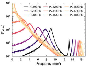
Figure 7: The dynamical structure factor, $S(\boldsymbol{q},\omega)$, calculated from MD for various pressures at 300. Here, $\boldsymbol{q}=\frac{2\pi}{a}(3/2,1/2,1/2)$.

The corresponding static structure factor is shown in Fig. 8. The static structure factor has the shape of a Lorentzian peak on a log-scale. The width of peak decreases when approaching the phase transition, indicating that the correlation length increases. Further, the value of static structure factor increases exponentially at the R-point as one approaches the phase transition pressure. This can be understood from the fact that the frequency of the R-tilt mode approaches zero at the phase transition and thus $S(\boldsymbol{q})$ diverges (cf. Eq. 5). Furthermore, the large values of $S(\boldsymbol{q},\omega)$ observed for higher pressures at low frequencies is directly related to the divergence of the static structure factor $S(\boldsymbol{q})$ (Fig. 8), as can be seen from Eq. 3.

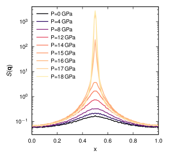
Figure 8: The structure factors, $S(\boldsymbol{q})$, calculated from MD for various pressures at 300. Here, $\boldsymbol{q}=\frac{2\pi}{a}(3/2,1/2,x)$

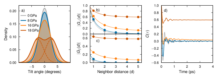
Figure 9: Properties of the tilt-angle $\theta^{\alpha}$ and its static and dynamic correlations from MD simulations at 300 and for four different pressures. The tilt-angle distribution and its correlations are averaged over $\alpha=x,y,z$ for $0$, $8$, and 16. For 18 they are only calculated over the direction $\alpha$ for which the tetragonal structure is tilted around. a) Distribution over observed tilt-angles. Solid lines corresponds to Gaussian fits with zero mean, or symmetric Gaussians with nonzero mean for 18. The dashed lines correspond to the two symmetric Gaussians for 18. b) and c) The static tilt-angle correlation functions, $G_{\parallel}(d)$ and $G_{\perp}(d)$, as a function of neighbor distance $d$. Solid lines are guides to the eye. c) The dynamic tilt-angle correlation function $C(\tau)$ as defined in Eq. (7).

II.5 Tilt angle correlations - pressure dependency

Finally, we consider the tilt angle and its static and dynamic correlations as function of pressure, shown in Fig. 9. The highest pressure, 18, is located above 16.2, the pressure where the system transform from the cubic to the tetragonal phase. The data for 18 is therefore calculated using only the direction $\alpha$ for which the tetragonal structure is tilted around. For the three lower pressures the data are obtained by making an average of the three different $\alpha$ directions.

The distribution for the tilt angle $P(\theta)$ as function of pressure is shown in Fig. 9a. The distribution widens with increasing pressure. For 18, where the system has undergone the phase transition to the tetragonal phase, the distribution develops a symmetric double peak distribution. This can be fitted well with two Gaussians with mean values $\mu_{t}=\pm$2.65 and standard deviation $\sigma_{t}=\$2.19.

The static tilt-angle correlation function as a function of neighbor distance is shown in Fig. 9b. The static correlations increase as function of pressure and the decay distance increases. Above the phase transition the correlations do not decay to zero and the correlation function approaches the constant value

$$|G(d\rightarrow\infty)|=\frac{\left<\theta_{t}\right>\left<\theta_{t}\right>}{\left<\theta_{t}^{2}\right>}=\frac{\mu_{t}^{2}}{\mu_{t}^{2}+\sigma_{t}^{2}}=0.59$$

for 18, reflecting the (global) long-ranged tilting in the tetragonal phase.

Similar behavior is also seen in the dynamic tilt-angle autocorrelation function $C^{\alpha}(\tau)$ in Fig. 9c. For pressures below the phase transitions $C^{\alpha}(\tau)$ decays to zero in the long-time limit, whereas for 18 $C^{\alpha}(\tau)$ approaches the same constant value as the static correlation function, i.e., $C^{\alpha}(\tau\rightarrow\infty)=0.59$. It is interesting to note that just below the phase transition the decay time increases substantially. This has also been seen in similar simulation studies of halide perovskites [18, 26].

III Discussion

Structural instabilities and phase transitions in perovskite oxides are important and have therefore been investigated extensively. Strontium titanate SrTiO3 (STO) is generally considered to be a model perovskite for the study of soft mode-driven phase transitions [28, 29] and it may be instructive to compare the behavior of STO with BZO.

At ambient conditions STO is cubic and its antiferrodistortive transition to the tetragonal ($I4/mcm$) phase can be induced by either decreasing the temperature or increasing the pressure [30]. The pressure induced transition at room temperature occurs at 9.6 for STO [31]. The same type of transition also occurs in BZO but at a somewhat higher pressure [14, 16]. On the other hand, the temperature induced transition at ambient pressure only occurs in STO, not in BZO. In STO the R-tilt mode softens and at about 105 [28, 32] it approaches zero and the material undergoes a phase transition to the tetragonal structure. When approaching this phase transition from above the scattering intensity near the R-point increases dramatically and the scattering peak narrows substantially in $\boldsymbol{q}$-space [32].

Our results demonstrate that a similar mechanism is also at play in BZO and detected in the experiments by Levin et al. [13]. Yet in contrast to STO, one only reaches the initial narrowing of the peak as the phase transition never occurs at ambient pressure. The R-tilt mode softens but its frequency remains finite when the temperature goes to zero [5, 6]. Levin et al. [13] find a diffuse peak at the R-point with a width of 0.22. This magnitude corresponds roughly to the corresponding peak for STO at about 160, that is 50 above the transition to the tetragonal phase [32]. The “nanodomains” observed by Levin et al. [13] are thus dynamic correlations at the onset of a phase transition that never occurs in BZO at ambient pressures.

IV Conclusions

We have performed large scale MD simulations of barium zirconate, an oxide perovskite, using machine-learned potentials based on DFT calculations. Both the temperature and pressure dependence of the local and global structure and the dynamics were investigated, and compared with available electron diffraction results.

At ambient pressure it is now well established that BZO remains cubic down to zero Kelvin, although the R-tilt mode softens substantially [6]. Our MD simulations predict a softening from 9 at 300 to 3 at 40. We find that this mode softening gives rise to a clear oxygen related peak in the static structure factor at the R-point, which explains the superlattice reflection observed by Levin et al. [13] using electron diffraction.

Levin et al. [13] state that the peak is only visible below about 80. However, we show that it does exist also at higher temperatures, albeit with weaker intensity. The present study strongly suggests that the disappearance of the peak in the electron diffraction study at higher temperatures is due to the large background intensity from scattering of Ba and Zr at those temperatures. The oxygen related peak is the result of strongly correlated and dynamic tilting between neighboring ZrO6 octahedra. By investigating the tilt angle correlations we find that the spatial extent of the correlated motion at 40 is about 2 to 3 and with a short relaxation time of about 1. We therefore conclude that the oxygen peak observed at the R-point is purely of dynamic origin.

The pressure dependence at room temperature was also investigated. It is known that BZO undergoes a phase transition from the cubic to the tetragonal phase. Here, we obtain this transition at about 16 in the middle of the experimentally observed range. When approaching the phase transition from lower pressures, the frequency of the R-tilt mode approaches zero and close to the phase transition the motion becomes overdamped. At the same time the static structure factor at the R-point increases dramatically by several orders of magnitude. The dynamic tilt-angle autocorrelation function shows a rapid decay on the order of 1, but close to the transition, the correlation function also develops a component with a considerably slower decay. At the phase transition this decay goes over to a constant finite value. The static tilt-angle correlation function shows a similar behavior: The decay rate becomes longer and longer and the correlation function approaches a constant value at the phase transition.

The present study shows that large scale MD simulations based on a machine-learned potentials with near DFT accuracy can provide immensely detailed and accurate atomic scale information on the local structure and complex dynamics close to phase transitions.

V Methods

V.1 Reference calculations

The energy, forces, and virials are obtained for the training structures via DFT calculations as implemented in the Vienna ab-initio simulation package [33, 34, 35] using the projector-augmented wave [36, 37] setups in version 5.4.4 with a plane wave energy cutoff of 510. The considered valence configurations for Ba, Zr and O are $5s^{2}5p^{6}6s^{2}$, $4s^{2}4p^{6}4d^{2}5s^{2}$ and $2s^{2}2p^{2}$, respectively. The Brillouin zone is sampled with a Monkhorst-Pack grid, with the maximum distance between two points being 0.19 along the reciprocal lattice vectors. This leads to a 8x8x8 $\boldsymbol{k}$-point grid for the primitive cell with a lattice parameter of 4.20.

For the exchange-correlation functional we employ the van-der-Waals-density functional with consistent exchange (vdW-DF-cx) [38, 39], here abbreviated CX. This functional is a version of the vdW-DF method [40], with the aim of accurately capturing competing interactions in soft and hard materials [41, 42]. It has been applied to BaZrO3 before [4, 43] and been found to give a very good account of its structural and vibrational properties. In particular, the anharmonicity of the R-tilt mode at ambient pressure is well described compared to recent experiments on BaZrO3 [6], and so is the thermal expansion [43] (for more details see LABEL:sfig:lattice_parameters and LABEL:sfig:Rmode_frequency_XC).

V.2 Neuroevolution potential

We construct an NEP model for the potential energy surface using the iterative strategy outlined in Ref. 44. Training structures include cubic, tetragonal and rhombohedral primitive cells at different volumes and cell-shapes, MD structures in a 4x4x4 (320 atoms) supercell at temperatures up to 500 and pressures up to 40, structures with various tilt-modes imposed, cubic-tetragonal and tetragonal-tetragonal interface structures, and structures found by simulated annealing at different pressures. The MD structures are generated using an initial NEP model and are selected based on their uncertainty, which is estimated from the predictions of an ensemble of models [44]. The final NEP model used in the production runs is trained on all the available training data (see LABEL:sfig:active_learning). The NEP model accurately reproduces the energy-volume curves for the different phases, the phonon dispersions for the cubic phase as well as the static energy landscape of the tilt modes (R and M). More details pertaining to the validation of the NEP model including parity plots are provided in the Supporting Information.

V.3 Molecular dynamics

All MD simulations are run with gpumd [45]. In all simulations we employ a timestep of 1 and equilibration time of 50. For most simulations we use supercells comprising 24x24x24 cubic primitive cells ($\sim$ 70 thousand atoms). However, the static structure factor $S(\boldsymbol{q})$ is calculated from MD simulations with 144x144x144 cubic primitive cells ($\sim$ 15 million atoms) in order to achieve an adequate $\boldsymbol{q}$-point resolution. The static and dynamic structure factors are calculated from MD trajectories using the dynasor package [46].

The phase diagram is obtained from simulations in the NPT ensemble, static properties from simulations in the NVT ensemble, and dynamic properties from simulations in the NVE ensemble. NVT and NVE simulations are carried out with lattice parameters obtained from NPT simulations (see LABEL:sfig:lattice_parameters).

Data Availability

The NEP model for BaZrO3 constructed in this study as well as a database with the underlying DFT calculations is openly available via Zenodo at https://doi.org/10.5281/zenodo.8337182.

Supporting information

The supporting information provides details pertaining to the DFT calculations, the NEP construction and the validation of the NEP. Furthermore, the supporting information contains additional results and figures like thermal expansion, static structure factors, and more details on the local-tilt angles.

References

- Bhalla et al. [2000] A. Bhalla, R. Guo, and R. Roy, Materials Research Innovations 4, 3 (2000).
- Akbarzadeh et al. [2005] A. R. Akbarzadeh, I. Kornev, C. Malibert, L. Bellaiche, and J. M. Kiat, Physical Review B 72, 205104 (2005).
- Knight [2020] K. S. Knight, Journal of Materials Science 55, 6417 (2020).
- Perrichon et al. [2020] A. Perrichon, E. Jedvik Granhed, G. Romanelli, A. Piovano, A. Lindman, P. Hyldgaard, G. Wahnström, and M. Karlsson, Chemistry of Materials 32, 2824 (2020).
- Zheng et al. [2022] J. Zheng, D. Shi, Y. Yang, C. Lin, H. Huang, R. Guo, and B. Huang, Phys. Rev. B 105, 224303 (2022).
- Rosander et al. [2023] P. Rosander, E. Fransson, C. Milesi-Brault, C. Toulouse, F. Bourdarot, A. Piovano, A. Bossak, M. Guennou, and G. Wahnström, Phys. Rev. B 108, 014309 (2023).
- Chemarin et al. [2000] C. Chemarin, N. Rosman, T. Pagnier, and G. Lucazeau, Journal of Solid State Chemistry 149, 298 (2000).
- Karlsson et al. [2008] M. Karlsson, A. Matic, C. S. Knee, I. Ahmed, S. G. Eriksson, and L. Börjesson, Chemistry of Materials 20, 3480 (2008).
- Giannici et al. [2011] F. Giannici, M. Shirpour, A. Longo, A. Martorana, R. Merkle, and J. Maier, Chemistry of Materials 23, 2994 (2011).
- Lucazeau [2003] G. Lucazeau, Journal of Raman Spectroscopy 34, 478 (2003).
- Toulouse et al. [2019] C. Toulouse, D. Amoroso, C. Xin, P. Veber, M. C. Hatnean, G. Balakrishnan, M. Maglione, P. Ghosez, J. Kreisel, and M. Guennou, Phys. Rev. B 100, 134102 (2019).
- Lebedev and Sluchinskaya [2013] A. I. Lebedev and I. A. Sluchinskaya, Physics of the Solid State 55, 1941 (2013).
- Levin et al. [2021] I. Levin, M. G. Han, H. Y. Playford, V. Krayzman, Y. Zhu, and R. A. Maier, Physical Review B 104, 214109 (2021).
- Yang et al. [2014] X. Yang, Q. Li, R. Liu, B. Liu, H. Zhang, S. Jiang, J. Liu, B. Zou, T. Cui, and B. Liu, Journal of Applied Physics 115, 124907 (2014).
- Gim et al. [2022] D.-H. Gim, Y. Sur, Y. H. Lee, J. H. Lee, S. Moon, Y. S. Oh, and K. H. Kim, Materials 15, 4286 (2022).
- Toulouse et al. [2022] C. Toulouse, D. Amoroso, R. Oliva, C. Xin, P. Bouvier, P. Fertey, P. Veber, M. Maglione, P. Ghosez, J. Kreisel, and M. Guennou, Physical Review B 106, 064105 (2022).
- Sun et al. [2010] T. Sun, X. Shen, and P. B. Allen, Physical Review B 82, 224304 (2010).
- Fransson et al. [2023a] E. Fransson, P. Rosander, F. Eriksson, J. M. Rahm, T. Tadano, and P. Erhart, Communications Physics 6, 173 (2023a).
- Togo and Tanaka [2015] A. Togo and I. Tanaka, Scripta Materialia 108, 1 (2015).
- Zhao and Weidner [1991] Y. Zhao and D. J. Weidner, Physics and Chemistry of Minerals 18, 294–30 (1991).
- Neil W. Ashcroft and N. David Mermin [1976] Neil W. Ashcroft and N. David Mermin, Solid State Physics (Holt, Rinehart and Winston, 1976).
- Chou and Choi [2000] M. Y. Chou and M. Choi, Phys. Rev. Lett. 84, 3733 (2000).
- Peng [1998] L.-M. Peng, Acta Crystallographica Section A 54, 481 (1998).
- Stukowski [2009] A. Stukowski, Modelling and Simulation in Materials Science and Engineering 18, 015012 (2009).
- Wiktor et al. [2023] J. Wiktor, E. Fransson, D. Kubicki, and P. Erhart, Chemistry of Materials 35, 6737 (2023).
- Baldwin et al. [2023] W. J. Baldwin, X. Liang, J. Klarbring, M. Dubajic, D. Dell'Angelo, C. Sutton, C. Caddeo, S. D. Stranks, A. Mattoni, A. Walsh, and G. Csányi, Small , 2303565 (2023).
- Liang et al. [2023] X. Liang, J. Klarbring, W. J. Baldwin, Z. Li, G. Csányi, and A. Walsh, The Journal of Physical Chemistry C 127, 19141 (2023).
- Fleury et al. [1968] P. A. Fleury, J. F. Scott, and J. M. Worlock, Physical Review Letters 21, 16 (1968).
- Cowley [1996] R. A. Cowley, Philosophical Transactions of the Royal Society of London. Series A: Mathematical, Physical and Engineering Sciences 354, 2799 (1996).
- Weng et al. [2014] S.-C. Weng, R. Xu, A. H. Said, B. M. Leu, Y. Ding, H. Hong, X. Fang, M. Y. Chou, A. Bosak, P. Abbamonte, S. L. Cooper, E. Fradkin, S.-L. Chang, and T.-C. Chiang, EPL (Europhysics Letters) 107, 36006 (2014).
- Guennou et al. [2010] M. Guennou, P. Bouvier, J. Kreisel, and D. Machon, Phys. Rev. B 81, 054115 (2010).
- Holt et al. [2007] M. Holt, M. Sutton, P. Zschack, H. Hong, and T.-C. Chiang, Physical Review Letters 98, 065501 (2007).
- Kresse and Hafner [1993] G. Kresse and J. Hafner, Physical Review B 47, 558 (1993).
- Kresse and Furthmüller [1996a] G. Kresse and J. Furthmüller, Phys. Rev. B 54, 11169 (1996a).
- Kresse and Furthmüller [1996b] G. Kresse and J. Furthmüller, Comp. Mater. Sci. 6, 15 (1996b).
- Blöchl [1994] P. E. Blöchl, Physical Review B 50, 17953 (1994).
- Kresse and Joubert [1999] G. Kresse and D. Joubert, Phys. Rev. B 59, 1758 (1999).
- Dion et al. [2004] M. Dion, H. Rydberg, E. Schröder, D. C. Langreth, and B. I. Lundqvist, Phys. Rev. Lett. 92, 246401 (2004).
- Berland and Hyldgaard [2014] K. Berland and P. Hyldgaard, Physical Review B 89, 035412 (2014).
- Berland et al. [2015] K. Berland, V. R. Cooper, K. Lee, E. Schröder, T. Thonhauser, P. Hyldgaard, and B. I. Lundqvist, Reports on Progress in Physics 78, 066501 (2015).
- Berland et al. [2014] K. Berland, C. A. Arter, V. R. Cooper, K. Lee, B. I. Lundqvist, E. Schröder, T. Thonhauser, and P. Hyldgaard, The Journal of Chemical Physics 140, 18A539 (2014).
- Frostenson et al. [2022] C. M. Frostenson, E. J. Granhed, V. Shukla, P. A. T. Olsson, E. Schröder, and P. Hyldgaard, Electronic Structure 4, 014001 (2022).
- Granhed et al. [2020] E. J. Granhed, G. Wahnström, and P. Hyldgaard, Phys. Rev. B 101, 224105 (2020).
- Fransson et al. [2023b] E. Fransson, J. Wiktor, and P. Erhart, The Journal of Physical Chemistry C 127, 13773 (2023b).
- Fan et al. [2017] Z. Fan, W. Chen, V. Vierimaa, and A. Harju, Computer Physics Communications 218, 10 (2017).
- Fransson et al. [2021] E. Fransson, M. Slabanja, P. Erhart, and G. Wahnström, Advanced Theory and Simulations 4, 2000240 (2021).