Longitudinal Volumetric Study for the Progression of Alzheimer’s Disease from Structural MR Images

Abstract

Alzheimer’s Disease (AD) is primarily an irreversible neurodegenerative disorder affecting millions of individuals today. The prognosis of the disease solely depends on treating symptoms as they arise and proper caregiving, as there are no current medical preventative treatments. For this purpose, early detection of the disease at its most premature state is of paramount importance. This work aims to survey imaging biomarkers corresponding to the progression of Alzheimer’s Disease (AD). A longitudinal study of structural MR images was performed for given temporal test subjects selected randomly from the Alzheimer’s Disease Neuroimaging Initiative (ADNI) database. The pipeline implemented includes modern pre-processing techniques such as spatial image registration, skull stripping, and inhomogeneity correction. The temporal data across multiple visits spanning several years helped identify the structural change in the form of volumes of cerebrospinal fluid (CSF), grey matter (GM), and white matter (WM) as the patients progressed further into the disease. Tissue classes are segmented using an unsupervised learning approach using intensity histogram information. The segmented features thus extracted provide insights such as atrophy, increase or intolerable shifting of GM, WM and CSF and should help in future research for automated analysis of Alzheimer’s detection with clinical domain explainability.

1 Introduction

Reports show that 8.8 million Indians above the age of 60 live with dementia (an umbrella term for Alzheimer’s Disease), amounting to approximately 7.4% of the total population. It is projected that the number of dementia afflicted may increase to 16.9 million by 2036 with the rapid rise of correlated risk factors such as diabetes and hypertension, both under-treated in rural settings [1, 2]. Common AD symptoms include memory impairment, loss of cognitive function, depression and paranoia. Even though these symptoms inevitably worsen over time, those providing care feel more in control with an early diagnosis and seek assistance from support groups along with others who have experienced similar misfortunes [3]. A review published in 2013 states that the annual overhead cost of looking after a person with Alzheimer’s in India can reach heights of 2,02,450 in urban areas and 66,025 in rural areas, including intangible costs such as loss of productivity, medication cost, consultation and hospitalization [4].

German physicist Alois Alzheimer laid the foundations of most of the modern understanding of the underlying causes of this disorder when he noticed the common biomarkers through histological techniques on the brains of his diseased patients [5]. Recent technologies exist, such as MRI, which helps in visualising atrophy or change in tissue volume of such biomarkers over a period of time, or fMRI, which can identify high-resolution activation of different brain regions during various cognitive tasks [6]. Fig. 1 shows the example of an AD patient’s raw unprocessed brain slice in different planes obtained from MR imaging in a magnetization-prepared rapid gradient-echo (MP-RAGE) sequence.

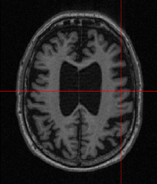
(a)

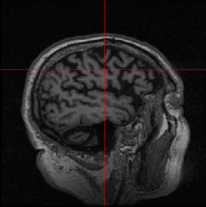
(b)

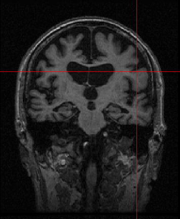
(c)

Figure 1: MP-RAGE T1 Weighted MR slices: (a) Axial plane (b) Sagittal plane (c) Coronal plane

1.1 Related Works

Multiple large-scale longitudinal studies have been carried out to investigate the causal connection between various AD indicators and the development of cognitive decline and dementia (e.g., ADNI, Australian Imaging) [7, 8]. Due to the dearth of publicly available datasets corresponding to the Indian populace, ADNI database was extensively used for our experimentation. Over the past two decades, several techniques have been applied to measuring brain atrophy in structural MRI, such as the boundary shift integral technique [9, 10], which uses a linear registration to align base and follow-up scans to track the change in brain boundary; or tensor-based morphometry (TBM) [11] which utilises non-linear image registration to map the volume change between the baseline and follow up images. Numerous machine-learning feature extraction techniques have also been studied for distinctive biomarker detection in the advent of AD, but most lack reproducibility and generalizability in the current scenario [12, 13, 14].

2 Methodology

We put forward a methodology to extract imaging features from MP-RAGE MRI images to include medical domain explainability for future group pattern analysis works. For each patient, a standard pipeline was implemented in the open-source R software (integrated with fslr [15]). Fig 2 represents a flowchart to elucidate the steps such as database formation, pre-processing of the images, and feature extraction. We have only analysed the volumetric changes of three particular tissues, namely, cerebrospinal fluid (CSF), grey matter (GM) and white matter (WM), over the course of multiple visits for a patient diagnosed with AD. These volumetric data thus obtained are considered to be the features of Alzheimer’s Disease.

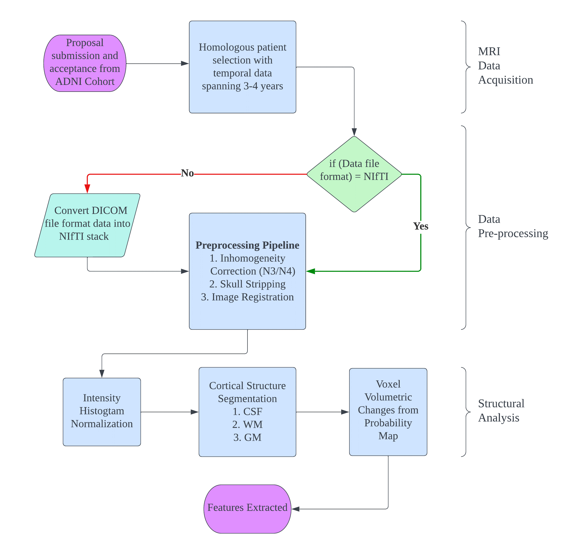
Figure 2: Flowchart for Structural Analysis in MP-RAGE MR images

2.1 Database Used

A representative dataset was created by selecting MP-RAGE structural MRI scans of AD patients at random after gaining access to the Alzheimer’s Disease Neuroimaging Initiative (ADNI - adni.loni.usc.edu), which was launched in 2003 and led by Principal Investigator Michael W. Weiner, MD. Patients were chosen such that they had at least three visits to track the change in the features of their disease progression.

2.2 Pre-processing

This section explains in detail the pre-processing paradigm implemented to align all the different visits. A wrapper script thus created with each of the steps enables us to easily process incoming files and perform the collection of transformations to further analyze our data.

2.2.1 File Preparation

The primary acquisition plane for each of the scans was sagittal, and the MP-RAGE scans downloaded from the ADNI website were in Digital Imaging and Communications in Medicine (DICOM) format. The DICOM format files (256 separated files for each slice) were first converted into a NIfTI stack (1 single file) to represent each visit for easier processing and visualization. In DICOM image files, the data comprises 2D layers, whereas NIfTI (Neuroimaging Informatics Technology Initiative) is a file format where images and other data are stored in a 3D structure. To access the DICOM files and convert them into a NIfTI file format, the $oro.dicom$ and $oro.nifti$ packages in R are used, which was introduced by Brandon Witcher et al. [16].

2.2.2 Inhomogeneity Correction

A significant issue faced while analyzing structural properties of the brain is the non-uniformity of intensity in structural MR images. Any low-frequency intensity which can be non-uniformly present in the data is referred to as inhomogeneity or bias field. A standard inhomogeneity correction algorithm known as the N4ITK or Improved Bias Correction [17] was used to remove low-frequency intensities. The image formation model of N3 is given by the following equation:

$$v(x)=u(x)f(x)+n(x)$$

where $v$ is the input image, $u$ is the uncorrupted actual image, $x$ is any location in the image, $f$ is the bias field, and $n$ is noise(which is assumed to be independent and gaussian). As the data is log-transformed and assumes a noise-free scenario ($n(x)=0$), the previous equation becomes

$$log(v(x))=log(u(x))+log(f(x))$$

The N4 algorithm then uses a robust B-spline approximation algorithm of the bias field and iterates until a convergence criterion is met where the modified bias field is approximately similar to the last performed iteration. After the updated transformation, the image is outputted back into the original file using inverse log transform. To visualise the effects of bias field correction Fig 3 shows a sample patient scan in all three planes by applying N4 bias correction using ANTsR library in R.

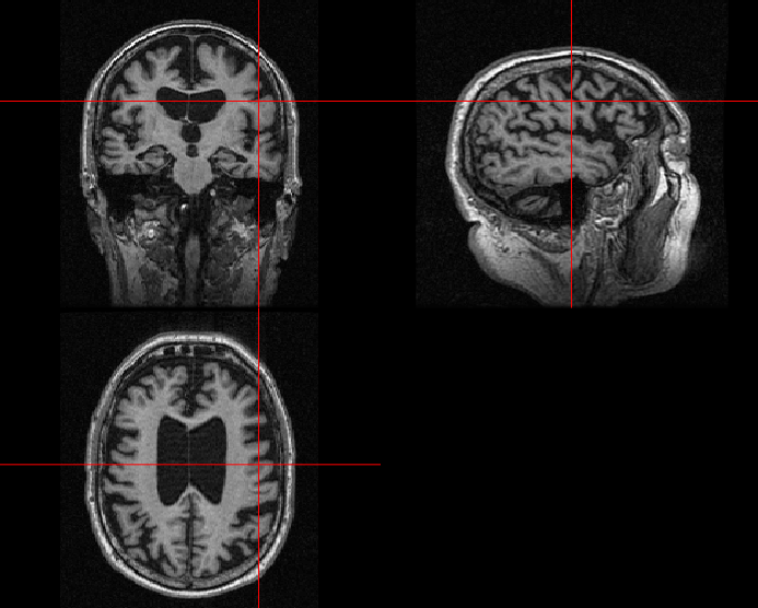
(a)

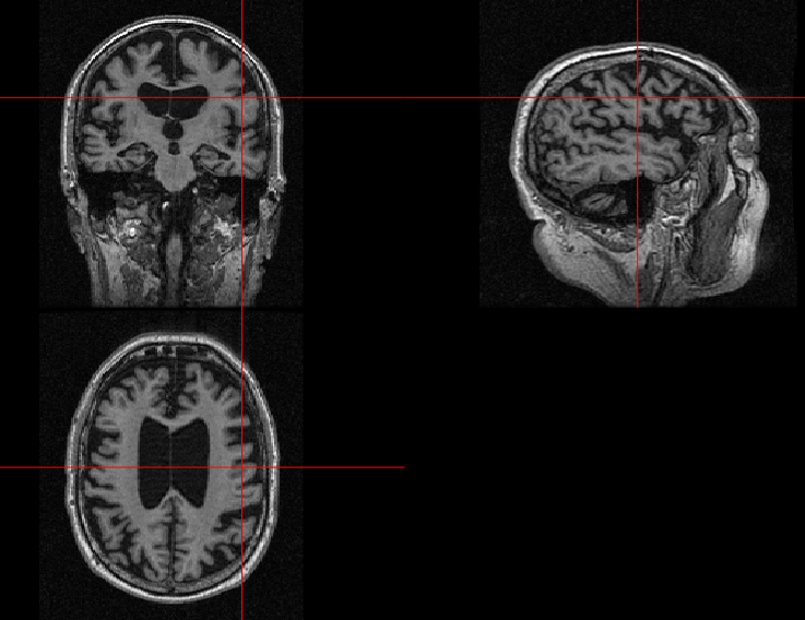
(b)

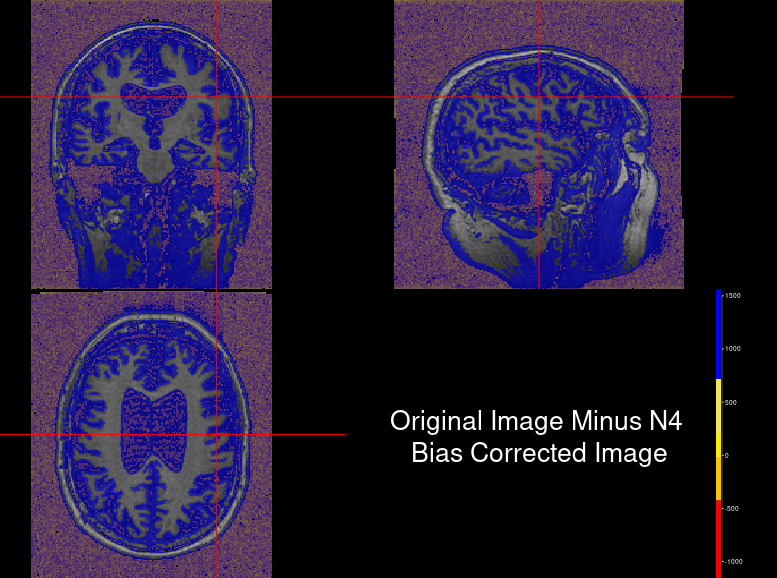
(c)

Figure 3: Inhomogeneity correction: (a) Source Scan (b) Bias Field Corrected Scan (c) Bias field corrected scan subtracted from source scan

Even though visually, there might not be a stark difference in the corrected scan, white and grey matter intensities are uniform in distribution compared to the source image. Fig 3(c) helps to visualize the difference where the blue gradient represents higher differences. It becomes imperative how there was a slowly varying field existing in the source image, which was removed in the corrected version.

2.2.3 Skull Stripping

This pre-processing technique removes the skull voxels from the T1-weighted MRI scan. To do this operation on the N4 bias-corrected image, FSL software [18] was used, which is integrated into R using the fslR package. Fslr performs required operations on NIfTI image objects using FSL commands and returns them as R objects [15]. The function $fslr::fslbet$ is readily available, which takes in the N4 corrected NIfTI image and calls the FSL BET function to perform skull stripping. Brain Extraction Tool (BET) [19] uses a deformable model that evolves to fit into the brain tissue surface locally adaptive model forces. To form a brain tissue mask which can be overlayed into the input scan, an NIfTI array is created and filled with binary ones using dimensions information from the header file. Secondly, the areas of the skull-stripped image containing the brain tissue were determined, or every pixel with a positive intensity value, because the skull stripping algorithm BET sets everything that is not brain to binary zeroes. A centre of gravity (CoG) of the extracted tissue was determined during the first iteration, and the algorithm was repeated by feeding the CoG as additional information to improve the skull stripping paradigm as one single iteration was observed to contain deformities. Bias correction, explained in the previous subsection, is essential for this step as the skull stripping algorithm heavily depends on the tissue intensities and a low variation in the field can hinder the output. The skull-stripped image thus obtained is shown in Fig 4.

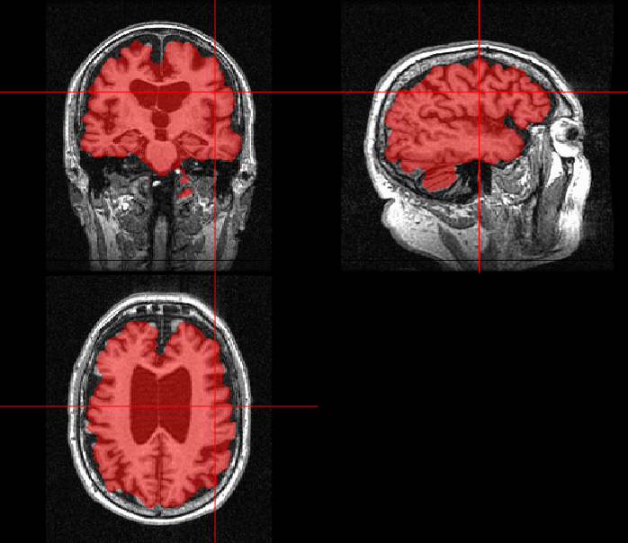
(a)

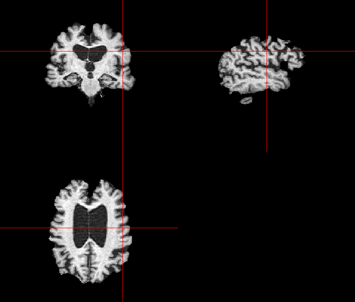
(b)

Figure 4: Skull Stripping: (a) Brain tissue mask overlay (b) Extracted brain tissue

2.2.4 Image Registration to Base Scan

The AD-affected patient scans selected with three or four visits need to be registered to make image locations such as voxels, and tissues have similar interpretations and align them spatially to compare changes. Each subsequent visit of each patient was co-registered to their source visit after performing inhomogeneity correction and skull stripping. Very few degrees of freedom are needed to register follow-up scans to the base scan as they belong to the same modality, so a rigid or affine registration is sufficient. Rigid registration is a linear registration technique containing six degrees of freedom and is represented by the equation: $T_{rigid}(v)=R_{v}+t$, where t is a translation vector $t=(t_{x},t_{y},t_{z})$ and R is a rotation matrix. All of the above operations were performed using the ANTsR package available in R.

2.3 Tissue Segmentation and Volume Extraction

After applying the necessary pre-processing steps described in the former subsections on the MR scans, a three-class tissue segmentation is performed using the FAST algorithm on the FSLR package integrated into R [15, 20]. The FAST algorithm, which uses the pipeline as described by Zhang et al., puts forward a hidden Markov random field model (HMRF) and an expectation maximization algorithm to perform probabilistic tissue segmentation. The intensity histogram is important for observing the working of the algorithm, so a sample intensity histogram is shown in Fig 5 of an Alzheimer’s affected patient’s MRI scan after preprocessing(no bias field, noise removed, skull stripped).

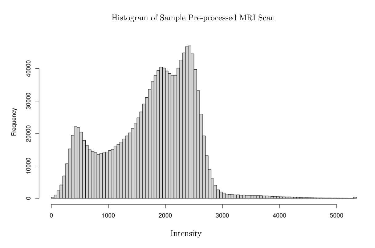
Figure 5: Intensity histogram of a sample AD patient scan after pre-processing

If the voxel frequency vs. intensity plot is observed, the three different tissue classes are apparent as three Gaussian peaks. The lowest intensity peak corresponds to Cerebrospinal Fluid (CSF), whereas the subsequent peaks determine the intensity peaks of grey matter (GM) and white matter (WM). A probability distribution for each tissue class is assigned such that $\mathcal{P}$(CSF) is near zero intensity levels; $\mathcal{P}$(GM) is of low to moderate levels of intensity; $\mathcal{P}$(WM) is of moderate to high levels of intensity. Spatial neighbourhood information or the HMRF model is used to segment each tissue class as simple classifiers like K-means do not use spatial entropy information, and we need a proper balance. The log probability model can be represented as $logp(intensity)+\beta logp(MRF)$, where $\beta$ is user-adjustable. Output files of the FAST algorithm provide three separate probability maps for corresponding tissue classes: $pve_{0}$, $pve_{1}$, and $pve_{2}$ for CSF, GM and WM, respectively. The $ortho2$ function in R is used to overlay the probability maps on the pre-processed T1 weighted image, as shown in Fig 6.

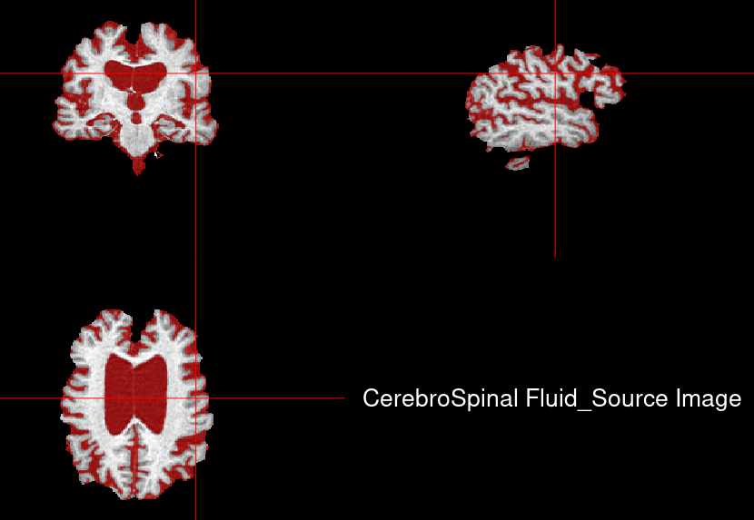
(a)

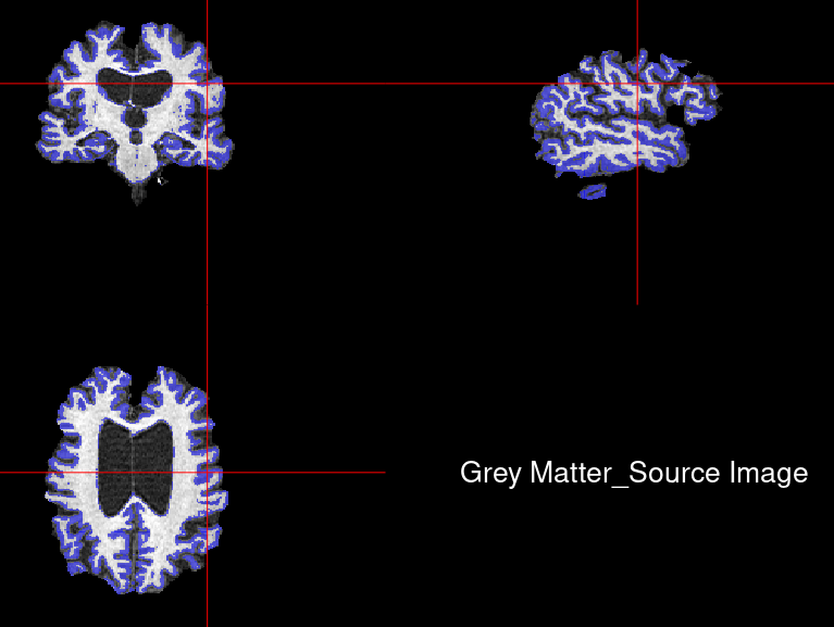
(b)

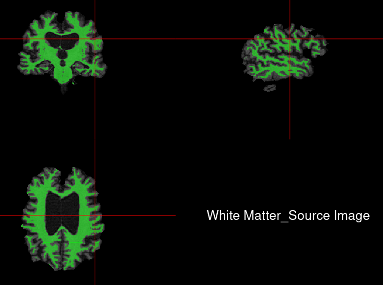
(c)

Figure 6: Segmentation of tissue classes of sample AD patient slice: (a)Cerebrospinal fluid (b) Grey Matter (c) White Matter

The changes in volumes of each patient for the tissue classes across three or four visits are observed and reported. These changes can be considered as relevant imaging features to understand the prognosis of Alzheimer’s disease.

3 Experimental Results

The above pipeline was iterated for each of the visits of the patients chosen from the ADNI database. $0.4$ was empirically chosen as the threshold for the output tissue probability maps after multiple experiments to calculate the volumes of each tissue class for the respective scans to extract features. First, the voxel dimension was calculated with a function called $voxdim$ available in $oro.nifti$ package. Then the number of voxels above the chosen threshold is calculated corresponding to the probability maps for each tissue class, given by $t_{vox}$. Finally, the volume is calculated in $mL$ with the equation $Volume=vox_{dim}\times(t_{vox}\div 1000)$, where $vox_{dim}$ is the voxel dimensions in $(ml)$ and the respective tissue voxels are $t_{vox}$ which is normalized to $1000$. The changes in volume in each tissue class were plotted in Fig 8 with each line depicting a patient after max scaling the data. Twenty-six patients’ volumetric data were observed, but after several permutations, fifteen of them were chosen to be plotted to show a majority trend (either increase in volume or decrease). The data is made available upon request to the authors for privacy concerns of ADNI guidelines.

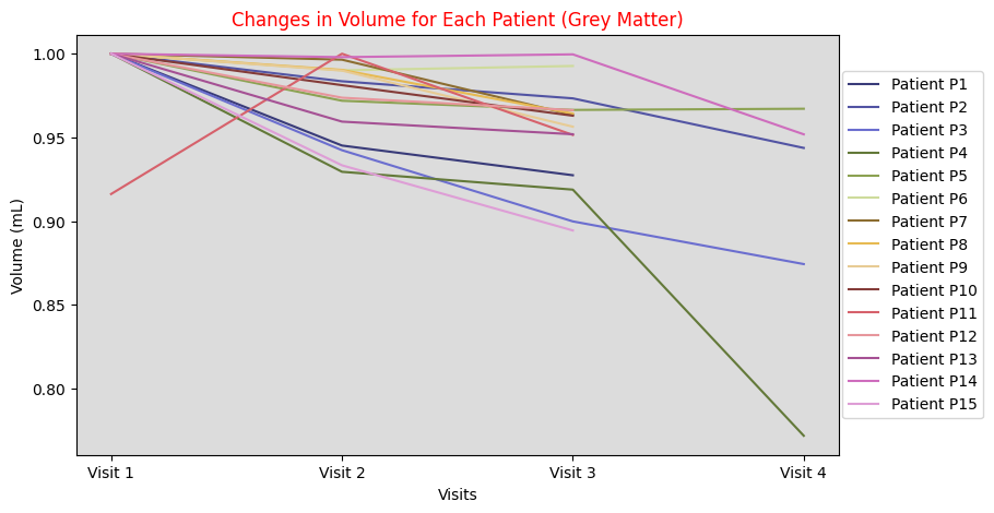
(a) Grey matter volume changes

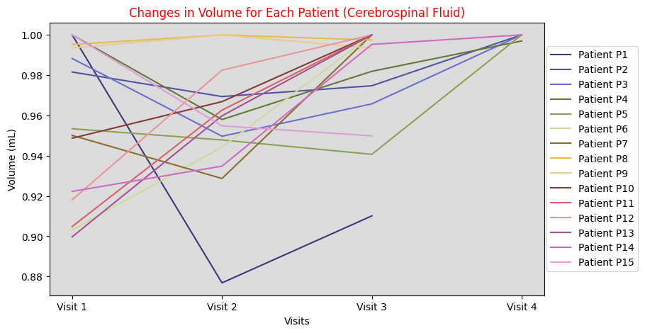
(b) Cerebrospinal fluid volume changes

Figure 7: Line plot for volume changes of each tissue class

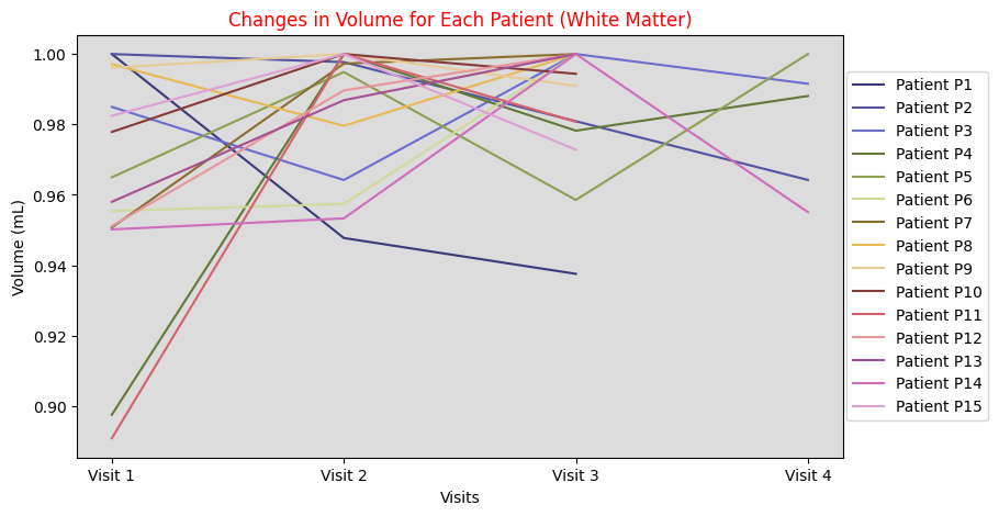
(a) White matter volume changes

Figure 8: Line plot for volume changes of each tissue class (cont.)

The mean volume and standard deviation for each chosen visit corresponding to each tissue class were calculated and reported in Table 1.

Table 1: Volumes of Each Tissue Class (Mean $\pm$ Standard Deviation)

Volume ($mL$)	Visit 1	Visit 2	Visit 3	Visit 4
Grey Matter	551.34 $\pm$ 61.56	538.01 $\pm$ 54.35	526.23 $\pm$ 54.01	497.42 $\pm$ 79.36
Cerebrospinal Fluid	383.67 $\pm$ 61.02	382.39 $\pm$ 64.50	391.09 $\pm$ 63.60	381.29 $\pm$ 42.86
White Matter	554.27 $\pm$ 69.86	553.63 $\pm$ 58.93	554.81 $\pm$ 58.27	549.02 $\pm$ 83.78

4 Discussion

We have created an easy-to-reproduce preprocessing pipeline and a wrapper script in R software to determine the volume from structural MRI scans of AD-affected patients for large-scale longitudinal analysis. Due to limited access to computational resources and an absence of Alzheimer’s datasets corresponding to the Indian landscape, we have considered MR scans of twenty-six patients from the ADNI database and compared their volume changes across three different tissue classes, namely cerebrospinal fluid (CSF), white matter (WM) and grey matter (GM). Of the twenty-six patients, fifteen were chosen, following a common pattern and their corresponding volumes were plotted across the three or four visits. The few inconsistencies can be attributed to several factors, such as responsiveness to symptom treatment, inaccurate MR scan acquisition, or incorrect segmentation due to spurious noise and other correlated abnormalities. In general, dementia is considered a grey matter degenerative disease as the common symptoms are congruent to a loss of grey matter volume [21]. Alzheimer’s affected patients show a massive loss in grey matter volume when compared to normal control counterparts. Our experimented volumes are consistent with clinical findings as we observe a general decline in GM volume, as shown in Fig 7(a) over a patient’s prognosis across several visits. Similarly, when Fig 7(b) is observed, it is imperative that an intolerable CSF shifting should also be considered as a common biomarker for Alzheimer’s Disease [22]. Fig 8(a) shows the white matter volume changes in AD patients, and even though a majority trend could not be identified from the line plot, specific abnormalities such as hyperintensities and lesion formation have been analyzed for their correlation with Alzheimer’s in multiple studies [23, 24].

The mean and standard deviation of each volume calculated and reported in Table 1 shed light on the behaviour of volume changes. As discussed above, grey matter is observed to follow a general decline across the four visits and can be heavily correlated with Alzheimer’s Disease. However, white matter and cerebrospinal fluid volumes stay consistent with marginal change in the mean volume but exhibit rapid shifts in the line plots.

This presented work can be considered as a first step for future large-scale analysis of the exhaustive MR scans of the ADNI dataset with more experimentation on different thresholds and more accurate pre-processing and segmentation techniques. Instead of black-box automated analysis from raw MR scans or intensive annotation methods, this added step of calculating additional imaging features related to the disease adds a layer of explainability with medical domain knowledge.

5 Acknowledgements

All the scans collected for analysis in preparation for this paper were accessed from the Laboratory of Neuro-imaging at the University of South California, which distributes ADNI data. ADNI is funded by the National Institute of Aging, the National Institute of Biomedical Imaging and Bioengineering, and through generous contributions from the following: AbbVie, Alzheimer’s Association; Alzheimer’s Drug Discovery Foundation; Araclon Biotech; BioClinica, Inc.; Biogen; Bristol-Myers Squibb Company; CereSpir, Inc.; Cogstate; Eisai Inc.; Elan Pharmaceuticals, Inc.; Eli Lilly and Company; EuroImmun; F. Hoffmann-La Roche Ltd and its affiliated company Genentech, Inc.; Fujirebio; GE Healthcare; IXICO Ltd.; Janssen Alzheimer Immunotherapy Research & Development, LLC.; Johnson & Johnson Pharmaceutical Research & Development LLC.; Lumosity; Lundbeck; Merck & Co., Inc.; Meso Scale Diagnostics, LLC.; NeuroRx Research; Neurotrack Technologies; Novartis Pharmaceuticals Corporation; Pfizer Inc.; Piramal Imaging; Servier; Takeda Pharmaceutical Company; and Transition Therapeutics. The study also deeply benefits from the open-source course on Introduction to Neurohacking in R offered by Johns Hopkins University.

References

- [1] Lee, J, Meijer, E, Langa, KM, et al. Prevalence of dementia in India: National and state estimates from a nationwide study. Alzheimer’s Dement. 2023; 19: 2898–2912. \doi10.1002/alz.12928
- [2] Ravindranath, V., and Sundarakumar, J. S. (2021). Changing demography and the challenge of dementia in India. Nature Reviews Neurology, 17(12), 747-758. \doi10.1038/s41582-021-00565-x
- [3] Kumar A, Sidhu J, Goyal A, et al. Alzheimer Disease. [Updated 2022 Jun 5]. In: StatPearls [Internet]. Treasure Island (FL): StatPearls Publishing
- [4] Rao, G., and Bharath, S. (2013). Cost of dementia care in India: Delusion or reality? Indian Journal of Public Health, 57(2), 71. \doi10.4103/0019-557X.114986
- [5] Stelzmann RA, Schnitzlein N, Murtagh FR : An English translation of Alzheimer’s paper, “über eine eigenartige Erkankung der Hirnrinde” Clinical Anatomy (1995)
- [6] Ogawa S, Lee TM, Kay AR, et al. Brain magnetic resonance imaging with contrast dependent on blood oxygenation. Proc Natl Acad Sci U S A. 1990; 87:9868.
- [7] Bondi, M. W., Edmonds, E. C., and Salmon, D. P. (2017). Alzheimer’s Disease: Past, Present, and Future. Journal of the International Neuropsychological Society: JINS, 23(9-10), 818. \doi10.1017/S135561771700100X
- [8] Jack, C. R., Knopman, D. S., Jagust, W. J., Shaw, L. M., Aisen, P. S., Weiner, M. W., … Trojanowski, J. Q. (2010). Hypothetical model of dynamic biomarkers of the Alzheimer’s pathological cascade. The Lancet Neurology, 9(1), 119–128. \doi10.1016/s1474-4422(09)70299-6
- [9] Leung K.K., Ridgway G.R., Ourselin S., Fox N.C. Consistent multi-time-point brain atrophy estimation from the boundary shift integral. Neuroimage. 2012; 59:3995–4005. \doi10.1016/j.neuroimage.2011.10.068
- [10] Freeborough P.A., Fox N.C. The boundary shift integral: an accurate and robust measure of cerebral volume changes from registered repeat MRI. IEEE Trans. Med. Imaging. 1997; 16:623–629 \doi10.1109/42.640753
- [11] Hua X., Hibar D.P., Ching C.R.K., Boyle C.P., Rajagopalan P., Gutman B.A., Leow A.D., Toga A.W., Jack C.R., Harvey D., Weiner M.W., Thompson P.M: Unbiased tensor-based morphometry (TBM): Improved robustness and sample size estimates for Alzheimer’s disease clinical trials. Neuroimage. 2013; 66:648–661 \doi10.1016/j.neuroimage.2012.10.086
- [12] Pan, D., Zeng, A., Jia, L., Huang, Y., Frizzell, T., and Song, X. (2020). Early Detection of Alzheimer’s Disease Using Magnetic Resonance Imaging: A Novel Approach Combining Convolutional Neural Networks and Ensemble Learning. Frontiers in Neuroscience, 14. \doi10.3389/fnins.2020.00259
- [13] Christian S., Antonio C., Petronilla B., Gilardi M. C., Aldo Q., Isabella C.: Magnetic resonance imaging biomarkers for the early diagnosis of Alzheimer’s disease: a machine learning approach. Frontiers in Neuroscience. 2015 9:307 \doi10.3389/fnins.2015.00307
- [14] Moradi E, Pepe A, Gaser C, Huttunen H, Tohka J; Alzheimer’s Disease Neuroimaging Initiative. Machine learning framework for early MRI-based Alzheimer’s conversion prediction in MCI subjects. Neuroimage. 2015 Jan 1; 104:398-412. \doi10.1016/j.neuroimage.2014.10.002
- [15] Muschelli, John & Sweeney, Elizabeth & Lindquist, Martin & Crainiceanu, Ciprian. (2015). Fslr: Connecting the FSL software with R. R Journal. 7. 163-175. \doi10.32614/RJ-2015-013.
- [16] Whitcher B, Schmid VJ, Thornton A (2011). ”Working with the DICOM and NIfTI Data Standards in R.” Journal of Statistical Software, 44(6), 1–28. \doi10.18637/jss.v044.i06.
- [17] Tustison, N. J., Avants, B. B., Cook, P. A., Zheng, Y., Egan, A., Yushkevich, P. A., & Gee, J. C. (2010). N4ITK: Improved N3 Bias Correction. IEEE Transactions on Medical Imaging, 29(6), 1310. \doi10.1109/TMI.2010.2046908
- [18] Jenkinson M, Beckmann CF, Behrens TE, Woolrich MW, Smith SM (2012). “FSL.” Neuroimage, 62(2), 782–790.
- [19] Smith, S. M. (2002). Fast robust automated brain extraction. Human Brain Mapping, 17(3), 143–155. \doi10.1002/hbm.10062
- [20] Zhang Y, Brady M, Smith S. Segmentation of brain MR images through a hidden Markov random field model and the expectation-maximization algorithm. IEEE Trans Med Imaging. 2001 Jan;20(1):45-57. \doi10.1109/42.906424
- [21] Wu, Zhanxiong, Yun Peng, Ming Hong, and Yingchun Zhang. ”Gray Matter Deterioration Pattern During Alzheimer’s Disease Progression: A Regions-of-Interest Based Surface Morphometry Study.” Frontiers in Aging Neuroscience 13, (2021): 593898. \doi10.3389/fnagi.2021.593898.
- [22] Paterson, R.W., Slattery, C.F., Poole, T. et al. Cerebrospinal fluid in the differential diagnosis of Alzheimer’s disease: clinical utility of an extended panel of biomarkers in a specialist cognitive clinic. Alz Res Therapy 10, 32 (2018). \doi10.1186/s13195-018-0361-3
- [23] Kao, Hui, et al. ”White Matter Changes in Patients with Alzheimer’S Disease and Associated Factors.” Journal of Clinical Medicine, vol. 8, no. 2, 2019, \doi10.3390/jcm8020167
- [24] Gootjes L., Teipel S., Zebuhr Y., Schwarz R., Leinsinger G., Scheltens P., Möller H.-J., Hampel H. Regional distribution of white matter hyperintensities in vascular dementia, alzheimer’s disease and healthy aging. Dement. Geriatr. Cogn. Disord. 2004;18:180–188. \doi10.1159/000079199