WeatherDepth: Curriculum Contrastive Learning for Self-Supervised Depth Estimation under Adverse Weather Conditions

Abstract

Depth estimation models have shown promising performance on clear scenes but fail to generalize to adverse weather conditions due to illumination variations, weather particles, etc. In this paper, we propose WeatherDepth, a self-supervised robust depth estimation model with curriculum contrastive learning, to tackle performance degradation in complex weather conditions. Concretely, we first present a progressive curriculum learning scheme with three simple-to-complex curricula to gradually adapt the model from clear to relative adverse, and then to adverse weather scenes. It encourages the model to gradually grasp beneficial depth cues against the weather effect, yielding smoother and better domain adaption. Meanwhile, to prevent the model from forgetting previous curricula, we integrate contrastive learning into different curricula. Drawn the reference knowledge from the previous course, our strategy establishes a depth consistency constraint between different courses towards robust depth estimation in diverse weather. Besides, to reduce manual intervention and better adapt to different models, we designed an adaptive curriculum scheduler to automatically search for the best timing for course switching. In the experiment, the proposed solution is proven to be easily incorporated into various architectures and demonstrates state-of-the-art (SoTA) performance on both synthetic and real weather datasets.

I INTRODUCTION

Depth estimation builds a bridge between 2D images and 3D scenes and has numerous potential applications such as 3D reconstruction [12], autonomous driving, etc. In recent years, due to the high costs of GT-depth collection from LiDARs and other sensors, researchers have turned to self-supervised solutions by exploiting photometric consistency between the depth-based reconstructed images and the target images. However, there is a sharp drop in depth precision when it comes to adverse weather conditions because weather particles spoil the consistency assumption and illumination variations produce an inevitable domain gap. Recent works tried to mitigate the performance degradation by restoring clear weather scenes [14], extracting features consistent with sunny conditions [29, 15], knowledge distillation from clear scenes [21, 8], etc. However these solutions do not account for the fact that weather comes in varying degrees and categories, and their data augmentation cannot reflect real situations well (Fig. 2), which hinders the potential of the estimation algorithm under weather conditions.

In this paper, we propose a self-supervised robust depth estimation model (named WeatherDepth) to address the above issues through curriculum contrastive learning. On the one hand, we simulate the progressive advances from clear to relatively adverse, and then adverse weather scenes, building three simple-to-complex curricula with adverse weather to different degrees. Concretely, we first train a base model on sunny data with clear structures to satisfy photometric consistency. This allows the model to obtain better-generalizable local optima for pre-training on more complex scenarios [2]. Then we optimize the model on relative adverse weather images with light effects, ground snow and water, which share a part of common regions with the clear domain and inspire the model to gradually grasp the depth cues against the missing textures and contrasts. Finally, we train the model on adverse data with the addition of weather particles (e.g., raindrops), further boosting the capability of handling complex noise patterns and violations of self-supervised assumptions.

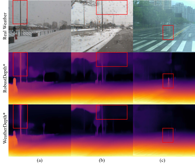
Figure 1: Typical examples on real weather images. Compared with Robust-Depth* (the SoTA robust depth estimation model under adverse weather), our WeatherDepth* produces more accurate results against (a) snowflakes, (b) raindrops on the lens, and (c) water surface reflections. Note both solutions adopt the same baseline model (MonoViT).

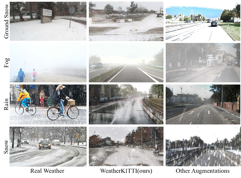
Figure 2: Comparison of simulated adverse weather. The other augmentations in the third column are from previous weather depth estimation studies [21, 14, 13], which also adopt data augmentation. Obviously, our WeatherKITTI augmentation is significantly more natural than their result.

On the other hand, predefined curriculum learning alone may lead to catastrophic forgetting [24] due to the substantial inter-domain difference in each stage. To this end, we embed light-weight contrastive learning designs in different curricula. Specifically, as shown in Fig. 3, we first establish one contrastive mode between two clear image with different traditional enhancements[11]. This forces the network to become more robust to this depth-irrelevant information and get prepared for the weather variation in later courses. Then, we build three more challenging contrastive modes between the sunny scene and randomly selected rainy/snowy/foggy weather scenes. It effectively prevents the network from solely focusing on resisting weather changes and completely biasing its domain to the new weather. In the last curriculum, we contrast three adverse weather against three relative adverse weather, constructing nine contrastive modes with the goal of improving the cross-weather robustness and relieving the problem of forgetting. These increasingly challenging contrastive modes( range from 1 to 3 to 9) formulate another curriculum learning process based on contrastive difficulty, which guides the training easily to be converged.

Moreover, we propose an adaptive curriculum scheduler to automatically switch curricula. It reduces manual intervention and produces smoother course transitions. To train an expected model and shrink the domain gap to real weather conditions, we combine GAN and PBR techniques [22] to build the WeatherKITTI dataset with diverse categories and magnitude of weather. Compared with existing augmented weather data [21, 13, 14], it renders a more realistic weather scene, as shown in Fig. 2.

Finally, we incorporate the proposed curriculum contrastive learning scheme into three popular depth estimation baselines (PlaneDepth, WaveletMonodepth, and MonoViT) to evaluate its effectiveness. Experimental results show the proposed WeatherDepth models outperform the existing SoTA solutions on both synthetic and real weather datasets. To our knowledge, this is the first work to apply curriculum contrastive learning to depth estimation. To sum up, the main contributions are summarized as follows:

• To adapt to adverse weather without knowledge forgetfulness, we propose a curriculum contrastive learning strategy with robust weather adaption. It can be applied to various SoTA depth estimation schemes and could be extended to other simple-to-complex prediction tasks.

• To reduce manual intervention and better adapt to different models, an adaptive curriculum scheduler is designed to automatically switch the course by searching for the best timing. Besides, we built the WeatherKITTI dataset to narrow the domain gap to real weather situations.

• We conduct extensive experiments to prove the universality of our curriculum contrastive learning scheme on various architectures and the superior performance over the existing SoTA solutions.

II Related work

II-A Self-supervised Depth Estimation

Since the pioneering work of Zhou et al. [31] showed that only using geometric constraints between consecutive frames can achieve excellent performance, researchers have continued to explore the cues and methods to train self-supervised models through videos [11, 25, 29] or stereo image pairs [19, 7, 10]. Afterward, methods including data augmentation[16], self-distillation[23, 1], indoor scenes aiding[27] etc. have been introduced to self-supervised models, pushing their inference performance closer to supervised models. Our model adopts both supervised training manners, monocular and stereo, to verify the scalability of our method.

II-B Adverse Condition Depth Estimation

Recently, the progress in depth prediction for typical scenes has opened up opportunities for tackling estimation in more challenging environments. Liu et al. [15] boost the nighttime monocular depth estimation (MDE) performance by using a Generative Adversarial Network (GAN) to render nighttime scenes and leveraging the pseudo-labels from day-time estimation to supervise the night-time training. Then, Zhao et al. [29] consider rainy nighttime additionally. In this work, to fully extract features from both scenes, they used two encoders trained separately on night and day image pairs and applied the consistency constraints at the feature and depth domains. The first MDE model under weather conditions was proposed in [21]. This work introduced a semi-augmented warp, which exploits the consistency between the clear frames while using the augmented prediction. Moreover, bi-directional contrast was incorporated in this work to improve the accuracy, although this doubles the training time. In [8], instead of using the KITTI dataset which only contains dry and sunny scenes, NuScenes and Oxford RobotCar datasets were adopted, for its real rainy and night scenarios. They first train a baseline on sunny scenes, then fix these net weights and transfer-train another network for weather scenes with day distill loss.

Besides the above methods that combine data augmentation and various strategies, there are also other solutions [14] trying to estimate depth after removing the weather influence on the image. Our approach synthesizes the strengths of previous works, utilizing a single end-to-end encoder-decoder network architecture to build an efficient and effective solution.

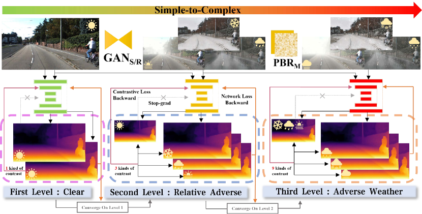
Figure 3: WeatherDepth pipeline Through three progressive stages, our model-agnostic approach can estimate depth reliably under weather environments. Except for the last stage, we input the loss of estimation model into the curriculum scheduler, in order to change the level properly. And we input image pairs $I_{aug}$ and $I_{cst}$ to obtain depth maps $D_{aug}$ and $D_{cst}$. $D_{cst}$ is detached as the contrastive target to compute contrastive loss, which is weighted and backpropagated together with the original loss.

III Method

In this section, we elaborate on the key components and algorithms of the proposed method.

III-A Preliminary

The proposed WeatherDepth is built on self-supervised depth estimation. Given a target input image $I\in\mathbb{R}^{C\times H\times W}$ and an auxiliary reference image $I^{\prime}$ from the stereo pair or adjacent frames, the self-supervised model $\mathcal{F}:I\rightarrow d\in\mathbb{R}^{H\times W}$ is expected to predict the disparity map $d$. With known baseline $b$ and focal length $f$, we compute the depth map $D=bf/d$. Then we can warp $I^{\prime}$ to the target view using the projected coordinates that are generated from $D$, relative camera poses $T_{I^{\prime}\rightarrow I}$ (from pose network or extrinsics) and intrinsics $K$:

$$\hat{I^{\prime}}=I^{\prime}\langle\text{Proj}(D,T_{I^{\prime}\rightarrow I},K)\rangle.$$ (1)

The above equation describes such a warping process, in which $\hat{I^{\prime}}$ denotes the warped image. The photometric reconstruction loss is then defined as:

$$l_{ph}(d)=\alpha\frac{1-\text{SSIM}(I,\hat{I^{\prime}})}{2}+\beta|I-\hat{I^{\prime}}|.$$ (2)

Based on stereo geometry, $l_{ph}$ equals 0 when $d$ is perfectly predicted. By minimizing the above loss, we can obtain the desired depth estimation. In addition, our WeatherDepth also adopts the semi-augmented warping from[21]:

$$\tilde{I^{\prime}}=I^{\prime}\left\langle\operatorname{Proj}\left(\tilde{D},T_{I^{\prime}\rightarrow I},K\right)\right\rangle,$$ (3)

where $\tilde{D}$ is the depth estimated using augmented images, $\tilde{I^{\prime}}$ is our semi-augmented warp result that will replace $\hat{I^{\prime}}$ to calculate $l_{ph}$. We leveraged the consistency between unaugmented images and the estimated depth of augmented images, avoiding the inconsistency between $\hat{I^{\prime}_{aug}}$ and $I$ caused by weather variations.

III-B Curriculum Selection

Due to the diversity of lighting and noise patterns in adverse weather, training directly on adverse weather data can easily lead to underfitting. To address this issue, we designed three curricula to gradually adapt to the new data domain. In curriculum designs, we obey the two principles. (1) The curriculum scenarios should follow the real-world weak-to-strong weather variation. (2) The curricula should be organized in a simple-to-complex order. To this end, we define our first curriculum as sunny scenes with slight adjustments on brightness, contrast, and saturation to make our model robust to these depth-invariant conditions. Then we simulate the relative adverse weather by incorporating the ground water reflections, ground snow, and droplets on the lens in the second course, which are not fully considered by previous works[8, 21]. These effects not only create wrong depth cues (like Fig. 1 (b,c)) but also change the texture of the origin scenes. In the last stage, we further introduce the raindrops, fog-like rain [22], the veiling effect, and snow streaks [5]. Because these particles are only visible in extremely adverse weather.

III-C Curriculum Contrastive Learning

To prevent the problem of forgetting the previous curricula, we embed contrastive learning into our curriculum learning process in an efficient manner.

As depicted in line 6 of Algorithm 1, in ContrastStep, we use the TrainStep model to directly infer the depth of $I_{cst}$. Here $I_{clr}$, $I_{cst}$ and $I_{aug}$ should have the same depth since they are different weather augmentations of the same image, and weather changes do not affect the scene itself. Moreover, prediction will be more accurate in previous levels, for weather variations are less severe. Therefore, as shown in Fig. 3, we can contrast the depth results from different curriculum stages to obtain the contrastive loss:

$$L_{\text{cst}}=\begin{cases}\log(|D_{aug}-\underline{D_{cst}}|+1),&\text{if }S_{aug}>S_{cst}\\ \log(|\underline{D_{aug}}-D_{cst}|+1),&\text{if }S_{cst}>S_{aug},\end{cases}$$ (4)

where $S_{aug}$ is the current curriculum stage, $S_{cst}$ is the stage of the contrastive weather. $D_{aug}$ and $D_{cst}$ are the depth predictions of the training image and contrastive inference respectively. The underlining signifies that the gradients are cut off during backpropagation. Then the final loss is:

$$L_{\text{backward}}=L_{\text{model}}+w_{curr}\cdot L_{\text{cst}},$$ (5)

where $L_{\text{model}}$ is the self-supervised model loss, $w_{curr}$ is the contrastive weight. Considering the model needs to adapt to weather changes when entering a new stage, we initialize it to a small value and update $w_{curr}$ each epoch according to:

$$w_{curr}=\begin{cases}w_{cst},&\text{if}\ r=0\\ \max(w_{max}w_{cst},\lambda w_{curr}),&\text{if }r\neq 0\ \text{and}\ r\mid 2\\ w_{curr},&\text{others},\end{cases}$$ (6)

where $\lambda$ is a constant $>1$. As the model gradually adapts to the curriculum stage, we want to steadily increase the consistency constraint. $r$ is the number of epochs trained in the current stage.

With the integration of contrast, our curriculum learning has considered both weather changes curricula and contrastive difficulty alterations.

Algorithm 1 Curriculum Scheduler for WeatherDepth

Input: Clear data $I^{clr}_{L},I^{clr}_{R}$, augmented data (only left) $I_{i}^{aug}$, contrast data (only left) $I_{i}^{cst}$, curriculum patience $P_{i}$

($i=1,2,3,$indicating the augmentation magnitude)

1:  Let level $l=1$, patience $p=0$

2:  for each epoch do

3:     Update contrastive weight $w_{curr}$

4:     for each batch do

5:        $D^{aug},L_{model}$=TrainStep$(I_{l}^{aug},I^{clr}_{L},I^{clr}_{R})$

6:        $D^{cst}$=InferenceStep$(I_{l}^{cst})$

7:        $L_{cst}$=ContrastStep$(D^{aug},D^{cst})$

8:        recordloss.Append($L_{model}$)

9:     end for

10:     recordkey.Append(Average(recordloss))

11:     if recordkey[-1] - recordkey [-2] $>$ threshold then

12:        $p=p+1$

13:     end if

14:     if $p\geq P_{i}$ then

15:        Reset $w_{curr}$ and $p=0$

16:        Switch to next-level data

17:        if $l$ = maxlevel and $P_{i}\geq 3$ then

18:           Load best epoch for the level $l$

19:        end if

20:        $l=l+1$

21:     end if

22:  end for

III-D Adaptive Curriculum Scheduler

As mentioned in [24], curriculum learning paradigms typically consist of two key components: the Difficulty Measurer and the Training Scheduler. The former is used to assign a learning priority to each data/task, while the latter decides when to introduce hard data into training. In this work, our Difficulty Measurer is pre-defined, whose benefits have been elaborated in section I. However, for different baseline models, the curriculum scheduler needs to be designed separately. A pre-defined switching mode (switching time) for a certain model may not adapt well to other networks. To this end, we check whether the network has fitted well in the current stage based on the change of self-supervised loss($L_{model}$), as shown in Fig. 3 and lines 10-20 in Algorithm 1. The contrastive loss is not included, because as stated before, the weight of contrastive learning itself varies across epochs, adding it would make the model extremely unstable. Actually, this strategy is inspired by early stopping methods[18], which effectively reduces training time and avoids overfitting at a certain stage.

III-E Method Scalability

To prove our expansiveness, we choose three popular models with tremendous differences in architecture as our baselines. The reasons are summarised as follows:

• WaveletMonodepth[19]: In this solution, wavelet transform is taken as the depth decoder, which trades off depth accuracy with speed. This is well suited for scenarios with different accuracy requirements.

• PlaneDepth[23]: This model uses Laplace mixture models based on orthogonal planes to estimate depth. It predicts depth for each plane respectively and computes the final depth by summing it over the Laplace distribution probabilities. Besides, PlaneDepth achieves current SoTA performance on self-supervised depth estimation.

• MonoViT[30]: Different from convolutional networks, MonoViT takes the transformer model as an encoder to improve image feature extraction. It represents the category of transformer-based models.

IV Experiments

IV-A Dataset

WeatherKITTI Dataset: Based on KITTI [9], we establish a weather-augmented dataset to enhance depth estimation models with generalization to real weather. It contains three kinds of most common weather types: rain, snow, and fog. As shown in Fig. 3, each weather type has two levels of magnitudes: relative adverse and adverse. The former includes light effects, ground snow and water, which are rendered by a CycleGAN model [32] trained on CADC [17], ACDC[20] and NuScenes[3] dataset. The latter further adds noticeable weather particles through physically-based rendering. Following SoTA weather rendering pipelines [22, 5], we generate adverse rains and snow masks. For foggy conditions, based on the atmospheric scattering model, we construct the second and third-stage foggy simulation augmentations under 150m and 75m visibility, respectively. Our rendered dataset covers all the images in the training and test scenes, totaling 284,304 (47,384$\times$6) images. To benchmark the robustness of models, we put the original KITTI and our weather-augmented KITTI together, named as the WeatherKITTI dataset.

DrivingStereo[26]: To characterize the performance of our models in real-world conditions, we use this dataset that provides 500 real rainy and foggy data images.

CADC: [17] is one of few snowy datasets, however, its data is in sequential order. Therefore, we sampled 1 in every 3 sequential images and obtained 510 images as test data. As shown in Fig. 1(a,b), this dataset contains real-world scenes with lens droplets, heavy snowfall, ground snow, etc. For depth GT generation, since LiDARs can be inaccurate under snowy conditions [28], we utilize the DROR[4] algorithm to filter out erroneous depths caused by snowflakes and generate the final depth GTs. In addition, invalid sky and ego-vehicle regions(without Lidar points) are removed, with a final image resolution of 1280$\times$540 pixels.

IV-B Implement Details

WaveletMonodepth, PlaneDepth, and MonoViT are three kinds of typical depth estimation models, and their performances are currently the best. Hence, we adapt the proposed curriculum contrastive learning scheme into these three baselines to validate our generalization, named as WeatherDepth, WeatherDepth^∗, WeatherDepth^† in Table I. Most hyperparameters(learning rate, optimizer, training image resolution, etc.) are the same as their origin implementation[30][23][19]. All models are trained on the WeatherKITTI dataset automatically with our scheduler. For stereo training, we use Eigen split [6]. As for monocular training, we follow Zhou split [31] with static scenes being removed. In our contrastive learning, we set $P_{1}=P_{2}=1$ and $w_{max}=10$ (all symbols are the same with Algorithm 1) for the three models. The model-specific minor modifications are shown in Table I. For all models, we strictly follow the original setup of [30, 23, 19] to train and evaluate our models. In particular, for MonoViT, we use monocular training for 30 epochs and test on $640\times 192$ resolution. The contrast depth is not detached during MonoViT training. For PlaneDepth, we only adopt the first training stage [23], training for 60 epochs in a stereo manner and testing with $1280\times 384$ resolution. For WaveletMonodepth, we train the Resnet-50 version for 30 epochs in a stereo manner and test with the resolution of $1024\times 320$.

In addition, to compare with Robust-Depth^∗ [21] fairly, we only adopt the WeatherDepth^∗ in comparative experiments as shown in Table II, because both Robust-Depth^∗ and WeatherDepth^∗ adopt the same baseline (MonoViT) and training/testing resolutions. As for WeatherDepth and WeatherDepth^†, they adopt different resolutions as used in [23, 19] and different baselines. To prevent unfair comparison, we only report the performance gains with the proposed curriculum contrastive learning scheme, shown in Table III and Table IV.

Table I: Model implementation details.

Baseline	Name	Threshold	$w_{cst}$
PlaneDepth	WeatherDepth	0	0.01
MonoViT	WeatherDepth∗	5e-4	0.02
WaveltMonoDepth	WeatherDepth†	0	0.1

IV-C WeatherKITTI Results

We show detailed comparative experiments between our method and current SoTA models in Table II(a). The Eigen raw split [6] is used for evaluation following common practice, and we report the average results under 7 different weather conditions.

In particular, Robust-Depth^∗ [21]is the latest SoTA model that tries to tackle weather conditions like us, but our WeatherDepth^∗ greatly outperforms it with the same baseline (MonoViT). These results sufficiently demonstrate that our method is able to handle weather variations and domain changes. As for the other two baselines, our WeatherDepth and WeatherDepth^† have also shown a significant gain in Table III (a) and Table IV (a), which implies that our strategy can be generalized to other typical depth estimation methods.

Table II: Quantitative Comparison against SoTA Models

Method	absrel	sqrel	rmse	rmselog	a1	a2	a3
(a) WeatherKITTI
MonoViT[30]	0.120	0.899	5.111	0.200	0.857	0.953	0.980
PlaneDepth[23]	0.150	1.360	6.513	0.277	0.757	0.891	0.945
Robust-Depth∗[21]	0.107	0.791	4.604	0.183	0.883	0.963	0.983
WeatherDepth∗	0.103	0.738	4.414	0.178	0.892	0.965	0.984
(b) DrivingStereo Dataset:Rain
MonoViT[30]	0.175	2.138	9.616	0.232	0.730	0.931	0.979
PlaneDepth [23]	0.220	3.302	11.671	0.278	0.654	0.883	0.965
Robust-Depth∗[21]	0.167	2.019	9.157	0.221	0.755	0.938	0.982
WeatherDepth∗	0.158	1.833	8.837	0.211	0.764	0.945	0.985
(c) CADC Dataset: Snow
MonoViT[30]	0.297	4.499	10.757	0.369	0.547	0.835	0.935
PlaneDepth[23]	0.356	4.903	11.453	0.405	0.447	0.749	0.908
Robust-Depth∗ [21]	0.298	5.550	11.481	0.369	0.590	0.853	0.932
WeatherDepth∗	0.279	4.632	10.699	0.357	0.597	0.857	0.938
(d) DrivingStereo Dataset: Fog
MonoViT[30]	0.109	1.206	7.758	0.167	0.870	0.967	0.990
PlaneDepth[23]	0.151	1.836	9.350	0.209	0.803	0.945	0.983
Robust-Depth∗ [21]	0.105	1.135	7.276	0.158	0.882	0.974	0.992
WeatherDepth∗	0.105	1.117	7.346	0.158	0.879	0.972	0.992

Table III: Incremental performance on PlaneDepth

Method	absrel	sqrel	rmse	rmselog	a1	a2	a3
(a) WeatherKITTI
PlaneDepth[23]	0.158	1.585	6.603	0.315	0.753	0.862	0.915
WeatherDepth	0.099	0.673	4.324	0.185	0.884	0.959	0.981
(b) DrivingStereo Dataset:Rain
PlaneDepth[23]	0.215	3.659	12.112	0.271	0.670	0.889	0.964
WeatherDepth	0.166	1.874	8.844	0.217	0.748	0.942	0.985
(c) CADC Dataset: Snow
PlaneDepth[23]	0.367	5.509	11.845	0.420	0.436	0.743	0.897
WeatherDepth	0.278	4.220	10.571	0.353	0.585	0.854	0.937
(d)) DrivingStereo Dataset: Fog
PlaneDepth[23]	0.122	1.416	8.306	0.179	0.847	0.961	0.990
WeatherDepth	0.123	1.404	7.679	0.172	0.859	0.968	0.992

Table IV: Incremental performance on WaveletMonodepth

Method	absrel	sqrel	rmse	rmselog	a1	a2	a3
(a) WeatherKITTI
WaveletMonodepth[19]	0.164	1.540	6.576	0.309	0.737	0.866	0.925
WeatherDepth†	0.103	0.777	4.532	0.191	0.878	0.958	0.981
(b) DrivingStereo Dataset:Rain
WaveletMonodepth[19]	0.280	4.604	13.231	0.339	0.570	0.819	0.922
WeatherDepth†	0.245	3.907	12.396	0.309	0.615	0.857	0.943
(c) CADC Dataset: Snow
WaveletMonodepth[19]	0.503	8.361	14.529	0.514	0.314	0.591	0.798
WeatherDepth†	0.394	6.828	13.293	0.443	0.427	0.714	0.876
(d)) DrivingStereo Dataset: Fog
WaveletMonodepth[19]	0.144	1.886	9.720	0.218	0.801	0.937	0.975
WeatherDepth†	0.140	1.784	8.893	0.199	0.818	0.950	0.984

IV-D Real Weather Scenes Results

To validate the ability to handle real-world weather, we follow [21] to use real-world weather data for testing. Note that all of our models are only trained on WeatherKITTI.

IV-D1 Rain

We show the quantitative results on real rainy data from the DrivingStereo dataset in Table II (b). Our method is still more accurate than the existing solutions, which demonstrates our model can adapt to the variations of rainy scenes. Especially, our scheme reduces the errors from water reflections and lens droplets as shown in Fig. 1(c).

IV-D2 Snow

As depicted in Table II (c), our method reaches the SoTA performance on the new CADC dataset. This further suggests that our method enables the depth estimation models to ignore the erroneous depth cues (Fig. 1(a)(b)) due to the progressive introduction of ground snow and snowflakes, which is very challenging for depth estimation tasks.

IV-D3 Fog

In Table II (d), we collect the results of fog scene evaluation for our model and SoTA frameworks. Unfortunately, Although our final model outperforms MonoViT itself, it falls slightly behind Robust-Depth. This is because the fog density in the DrivingStereo dataset is relatively light, while our model aims to address more adverse weather conditions (using more adverse fog augmentation). The domain adaptation of our model is biased after the second-stage fog augmentations.

In the (b-d) of Table III and Table IV, we can notice a similar trend as that of Table II, which further demonstrates the generalization capacity of the proposed strategy on different models(WaveletMonodepth, MonoViT, and PlaneDepth) and on different real weather datasets(Rain, Snow, and Fog).

IV-E Ablation Study

We have demonstrated the superiority of our method on synthetic and real adverse weather data. Next, we conduct experiments to validate the effectiveness of each component. For clarity, we only take WeatherDepth^∗ in the ablation study. As for the other models, they show similar performance and will be demonstrated in the supplement materials.

IV-E1 Learning Strategy

We define the direct mixed training manner as “w/o CC”, in which each weather condition has $1/n$ probability of being selected for training. As shown in Tables V(a-e), since mixed training attempts to estimate depth from erroneous depth cues introduced by weather variation, this strategy performs poorly on our WeatherKITTI dataset. Moreover, it degrades the performance across all three real weather scenes, further validating the effectiveness of our proposed curriculum contrastive learning.

Table V: Quantitative Results on Ablation Study

Method	absrel	sqrel	rmse	rmselog	a1	a2	a3
(a) WeatherKITTI
MonoViT[30]	0.120	0.899	5.111	0.200	0.857	0.953	0.980
WeatherDepth∗ w/o CC	0.105	0.833	4.554	0.180	0.893	0.964	0.983
WeatherDepth∗ w/o C	0.104	0.772	4.527	0.181	0.890	0.964	0.983
WeatherDepth∗	0.103	0.738	4.414	0.178	0.892	0.965	0.984
(b) DrivingStereo Dataset:Rain
MonoViT[30]	0.175	2.138	9.616	0.232	0.730	0.931	0.979
WeatherDepth∗ w/o CC	0.163	1.949	9.124	0.216	0.759	0.944	0.984
WeatherDepth∗ w/o C	0.156	1.755	8.916	0.212	0.768	0.945	0.985
WeatherDepth∗	0.158	1.833	8.837	0.211	0.764	0.945	0.985
(c) CADC Dataset: Snow
MonoViT[30]	0.297	4.499	10.757	0.369	0.547	0.835	0.935
WeatherDepth∗ w/o CC	0.305	5.967	11.846	0.373	0.582	0.847	0.929
WeatherDepth∗ w/o C	0.306	5.476	11.261	0.371	0.562	0.843	0.934
WeatherDepth∗	0.279	4.632	10.699	0.357	0.597	0.857	0.938
(d)) DrivingStereo Dataset: Fog
MonoViT[30]	0.109	1.206	7.758	0.167	0.870	0.967	0.990
WeatherDepth∗ w/o CC	0.112	1.282	7.511	0.163	0.873	0.970	0.992
WeatherDepth∗ w/o C	0.106	1.145	7.434	0.161	0.880	0.971	0.991
WeatherDepth∗	0.110	1.195	7.323	0.160	0.878	0.973	0.992
(e) KITTI (only sunny scenes)
MonoViT[30]	0.099	0.708	4.372	0.175	0.900	0.967	0.984
WeatherDepth∗ w/o CC	0.104	0.826	4.532	0.179	0.896	0.965	0.983
WeatherDepth∗ w/o C	0.100	0.702	4.445	0.177	0.894	0.965	0.984
WeatherDepth∗	0.099	0.698	4.330	0.174	0.897	0.967	0.984

IV-E2 Robustness on Sunny Condition

As reported in Table V(a-d), WeatherDepth^∗ without contrastive learning integration (termed as “w/o C”) shows a competitive performance with our final model on real and synthesized weather data. However, its performance on sunny days sharply declines as shown illustrated in Table V(e). In other words, without contrastive learning, the network only carries on weather domain transferring and loses the previous knowledge to tackle the sunny scenes. With our curriculum contrastive learning, our performance(trained on WeatherKITTI) on sunny data even outperforms the MonoViT[30](that trained on sunny data), which further suggests that our training manner gives robust depth results in any conditions.

IV-E3 Efficient Contrastive Learning

We incorporate the contrastive strategy of Robust-Depth and our contrastive scheme into the ResNet-18-based WaveletMonodepth model and train for 30 epochs on a 2080ti GPU. As shown in Table VI, our training time increases by less than 20% compared to no contrastive learning, while the Robust-Depth nearly doubles the training time due to bilateral propagation and image reconstruction. This validates that our method addresses performance degradation under weather conditions in a more efficient mode.

Table VI: Verify the efficiency of our Contrast Learning Manner

Contrast Method	Robust-Depth Way	WeatherDepth Way	No Contrast
Training Time	20h02m41s	12h10m07s	10h39m25s

V Conclusion

In this paper, we propose WeatherDepth, a self-supervised robust depth estimation strategy that employs curriculum contrastive learning to effectively tackle performance degradation in complex weather conditions. Our model progressively adapts to adverse weather scenes through a curriculum learning scheme and is further combined with contrastive learning to prevent knowledge forgetfulness. To narrow the weather domain gap, we also build the WeatherKITTI dataset to help models better adapt to real weather scenarios. Through extensive experiments, we demonstrated the effectiveness of our WeatherDepth against various architectures and its superior performance over existing SoTA solutions.

References

- [1] Juan Luis Gonzalez Bello and Munchurl Kim. Self-supervised deep monocular depth estimation with ambiguity boosting. IEEE Transactions on Pattern Analysis and Machine Intelligence, 44(12):9131–9149, 2022.
- [2] Yoshua Bengio, Jérôme Louradour, Ronan Collobert, and Jason Weston. Curriculum learning. In International Conference on Machine Learning, 2009.
- [3] Holger Caesar, Varun Bankiti, Alex H. Lang, Sourabh Vora, Venice Erin Liong, Qiang Xu, Anush Krishnan, Yu Pan, Giancarlo Baldan, and Oscar Beijbom. nuscenes: A multimodal dataset for autonomous driving, 2020.
- [4] Nicholas Charron, Stephen Phillips, and Steven Waslander. De-noising of lidar point clouds corrupted by snowfall. pages 254–261, 05 2018.
- [5] Wei-Ting Chen, Hao-Yu Fang, Cheng-Lin Hsieh, Cheng-Che Tsai, I Chen, Jian-Jiun Ding, Sy-Yen Kuo, et al. All snow removed: Single image desnowing algorithm using hierarchical dual-tree complex wavelet representation and contradict channel loss. In Proceedings of the IEEE/CVF International Conference on Computer Vision, pages 4196–4205, 2021.
- [6] David Eigen, Christian Puhrsch, and Rob Fergus. Depth map prediction from a single image using a multi-scale deep network, 2014.
- [7] Ravi Garg, Vijay Kumar BG, Gustavo Carneiro, and Ian Reid. Unsupervised cnn for single view depth estimation: Geometry to the rescue, 2016.
- [8] Stefano Gasperini, Nils Morbitzer, HyunJun Jung, Nassir Navab, and Federico Tombari. Robust monocular depth estimation under challenging conditions. In Proceedings of the IEEE/CVF International Conference on Computer Vision, 2023.
- [9] Andreas Geiger, Philip Lenz, and Raquel Urtasun. Are we ready for autonomous driving? the kitti vision benchmark suite. In 2012 IEEE conference on computer vision and pattern recognition, pages 3354–3361. IEEE, 2012.
- [10] Clément Godard, Oisin Mac Aodha, and Gabriel J. Brostow. Unsupervised monocular depth estimation with left-right consistency, 2017.
- [11] Clément Godard, Oisin Mac Aodha, Michael Firman, and Gabriel Brostow. Digging into self-supervised monocular depth estimation, 2019.
- [12] Shahram Izadi, David Kim, Otmar Hilliges, David Molyneaux, Richard Newcombe, Pushmeet Kohli, Jamie Shotton, Steve Hodges, Dustin Freeman, Andrew Davison, et al. Kinectfusion: real-time 3d reconstruction and interaction using a moving depth camera. In Proceedings of the 24th annual ACM symposium on User interface software and technology, pages 559–568, 2011.
- [13] Lingdong Kong, Yaru Niu, Shaoyuan Xie, Hanjiang Hu, Lai Xing Ng, Benoit R. Cottereau, Ding Zhao, Liangjun Zhang, Hesheng Wang, Wei Tsang Ooi, Ruijie Zhu, Ziyang Song, Li Liu, Tianzhu Zhang, Jun Yu, Mohan Jing, Pengwei Li, Xiaohua Qi, Cheng Jin, Yingfeng Chen, Jie Hou, Jie Zhang, Zhen Kan, Qiang Ling, Liang Peng, Minglei Li, Di Xu, Changpeng Yang, Yuanqi Yao, Gang Wu, Jian Kuai, Xianming Liu, Junjun Jiang, Jiamian Huang, Baojun Li, Jiale Chen, Shuang Zhang, Sun Ao, Zhenyu Li, Runze Chen, Haiyong Luo, Fang Zhao, and Jingze Yu. The robodepth challenge: Methods and advancements towards robust depth estimation, 2023.
- [14] Younkwan Lee, Jihyo Jeon, Yeongmin Ko, Byunggwan Jeon, and Moongu Jeon. Task-driven deep image enhancement network for autonomous driving in bad weather, 2021.
- [15] Lina Liu, Xibin Song, Mengmeng Wang, Yong Liu, and Liangjun Zhang. Self-supervised monocular depth estimation for all day images using domain separation, 2021.
- [16] Rui Peng, Ronggang Wang, Yawen Lai, Luyang Tang, and Yangang Cai. Excavating the potential capacity of self-supervised monocular depth estimation, 2021.
- [17] Matthew Pitropov, Danson Evan Garcia, Jason Rebello, Michael Smart, Carlos Wang, Krzysztof Czarnecki, and Steven Waslander. Canadian adverse driving conditions dataset. The International Journal of Robotics Research, 40(4-5):681–690, 2021.
- [18] Lutz Prechelt. Early stopping-but when? In Neural Networks: Tricks of the trade, pages 55–69. Springer, 2002.
- [19] Michaël Ramamonjisoa, Michael Firman, Jamie Watson, Vincent Lepetit, and Daniyar Turmukhambetov. Single image depth prediction with wavelet decomposition. In Proceedings of the IEEE/CVF Conference on Computer Vision and Pattern Recognition, June 2021.
- [20] Christos Sakaridis, Dengxin Dai, and Luc Van Gool. Acdc: The adverse conditions dataset with correspondences for semantic driving scene understanding. In Proceedings of the IEEE/CVF International Conference on Computer Vision, pages 10765–10775, 2021.
- [21] Kieran Saunders, George Vogiatzis, and Luis Manso. Self-supervised monocular depth estimation: Let’s talk about the weather, 2023.
- [22] Maxime Tremblay, Shirsendu Sukanta Halder, Raoul de Charette, and Jean-François Lalonde. Rain rendering for evaluating and improving robustness to bad weather. International Journal of Computer Vision, 129(2):341–360, sep 2020.
- [23] Ruoyu Wang, Zehao Yu, and Shenghua Gao. Planedepth: Self-supervised depth estimation via orthogonal planes, 2023.
- [24] Xin Wang, Yudong Chen, and Wenwu Zhu. A survey on curriculum learning. IEEE Transactions on Pattern Analysis and Machine Intelligence, 44(9):4555–4576, 2022.
- [25] Jamie Watson, Oisin Mac Aodha, Victor Prisacariu, Gabriel Brostow, and Michael Firman. The Temporal Opportunist: Self-Supervised Multi-Frame Monocular Depth. In Computer Vision and Pattern Recognition (CVPR), 2021.
- [26] Guorun Yang, Xiao Song, Chaoqin Huang, Zhidong Deng, Jianping Shi, and Bolei Zhou. Drivingstereo: A large-scale dataset for stereo matching in autonomous driving scenarios. In IEEE Conference on Computer Vision and Pattern Recognition (CVPR), 2019.
- [27] Zehao Yu, Lei Jin, and Shenghua Gao. P 2 net: Patch-match and plane-regularization for unsupervised indoor depth estimation. In European Conference on Computer Vision, pages 206–222. Springer, 2020.
- [28] Yuxiao Zhang, Alexander Carballo, Hanting Yang, and Kazuya Takeda. Perception and sensing for autonomous vehicles under adverse weather conditions: A survey. ISPRS Journal of Photogrammetry and Remote Sensing, 196:146–177, feb 2023.
- [29] Chaoqiang Zhao, Yang Tang, and Qiyu Sun. Unsupervised monocular depth estimation in highly complex environments, 2022.
- [30] Chaoqiang Zhao, Youmin Zhang, Matteo Poggi, Fabio Tosi, Xianda Guo, Zheng Zhu, Guan Huang, Yang Tang, and Stefano Mattoccia. MonoViT: Self-supervised monocular depth estimation with a vision transformer. In 2022 International Conference on 3D Vision (3DV). IEEE, sep 2022.
- [31] Tinghui Zhou, Matthew Brown, Noah Snavely, and David G. Lowe. Unsupervised learning of depth and ego-motion from video, 2017.
- [32] Jun-Yan Zhu, Taesung Park, Phillip Isola, and Alexei A Efros. Unpaired image-to-image translation using cycle-consistent adversarial networks. In Proceedings of the IEEE international conference on computer vision, pages 2223–2232, 2017.