Logic-guided Deep Reinforcement Learning for Stock Trading

Abstract.

Deep reinforcement learning (DRL) has revolutionized quantitative finance by achieving excellent performance without significant manual effort. Whereas we observe that the DRL models behave unstably in a dynamic stock market due to the low signal-to-noise ratio nature of the financial data. In this paper, we propose a novel logic-guided trading framework, termed as SYENS (Program Synthesis-based Ensemble Strategy). Different from the previous state-of-the-art ensemble reinforcement learning strategy which arbitrarily selects the best-performing agent for testing based on a single measurement, our framework proposes regularizing the model’s behavior in a hierarchical manner using the program synthesis by sketching paradigm. First, we propose a high-level, domain-specific language (DSL) that is used for the depiction of the market environment and action. Then based on the DSL, a novel program sketch is introduced, which embeds human expert knowledge in a logical manner. Finally, based on the program sketch, we adopt the program synthesis by sketching paradigm and synthesize a logical, hierarchical trading strategy. We evaluate SYENS on the 30 Dow Jones stocks under the cash trading and the margin trading settings. Experimental results demonstrate that our proposed framework can significantly outperform the baselines with much higher cumulative return and lower maximum drawdown under both settings.

1. Introduction

Deep reinforcement learning (DRL) has achieved great performance in many areas, e.g., stock trading (Ee et al., 2020; Nan et al., 2022), portfolio allocation(Guan and Liu, 2021; Cui et al., 2023), robotics (Polydoros and Nalpantidis, 2017; Huang et al., 2019), software testing (Zheng et al., 2021, 2019; Cao et al., 2021), etc. Concisely, the idea is to model the task as a Markov decision process (MDP) and optimize the agent’s policy so as to maximize the expected return. Despite its great success, it is found that the DRL model suffers from a lack of robustness under noisy real-world environments, for example, the stock market environment, which is known for its low signal-to-noise ratio (SNR) (Liu et al., 2022).

In order to improve the DRL strategies’ robustness, the previous state-of-the-art method proposes using the ensemble reinforcement learning paradigm (Yang et al., 2020). Yang et al. introduce an ensemble method that combines three deep reinforcement learning algorithms (i.e., Advantage Actor Critic (A2C) (Mnih et al., 2016), Proximal Policy Optimization (PPO) (Schulman et al., 2017) and Deep Deterministic Policy Gradient (DDPG) (Mnih et al., 2016; Lillicrap et al., 2015)). The idea is to select the best-performing agent using a validation rolling window in terms of Sharpe ratio (Sharpe, 1998) and use it to predict and trade for the next quarter. Experimental results validate the effectiveness of their approach which achieves a higher Sharpe ratio than all the subpolicies, min-variance portfolio allocation strategy, and the Dow Jones Industrial Average (DJIA). Yet we observe that though this ensemble approach manages to improve over the baselines, it is still quite sensitive to market turbulence and is likely to suffer from a large drawdown when encountering a bear market environment.

To mitigate the above-mentioned issue, in this paper, we propose a novel program synthesis-based ensemble method, called Program Synthesis-based Ensemble Strategy (SYENS). The idea is to represent the trading strategy in a logical, hierarchical form using a programming language. Specifically, to generate such a programmatic strategy, our method proposes using the program synthesis by sketching paradigm (Solar-Lezama, 2008). We first introduce a novel domain-specific language (DSL) which contains different language constructs for expressing decision-making logic. Then we construct a program sketch based on the DSL, which embeds the fundamental expert knowledge. The program sketch serves as the backbone of the high-level strategy which describes the stock market dynamics and guides the ensemble. Finally, we incorporate the subpolicies as the low-level strategy for the ensemble and optimize the framework using program synthesis techniques. The logical and hierarchical nature of the SYENS framework allows it to express its reasoning process with explicit cause-effect logic, therefore boosting its robustness. Furthermore, beyond the cash trading setting used by the previous work, we also implement the margin trading mechanism and evaluate SYENS and the baselines under both settings.

Our contributions are threefold. We propose a novel hierarchical logic-guided DRL framework for stock trading, called SYENS. The key idea is to utilize the program synthesis by sketching paradigm to generate a programmatic strategy in a human-readable form. We implement the margin trading mechanism to evaluate models’ effectiveness beyond the cash trading mechanism. Extensive experiments under both the cash trading and margin trading settings demonstrate the effectiveness of SYENS in improving robustness with much higher cumulative return and lower maximum drawdown.

2. Preliminary

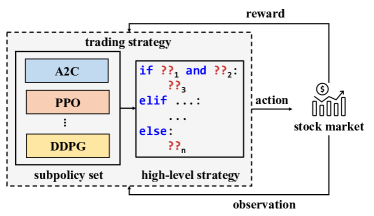
Figure 1. Overview of the SYENS backbone model. The model consists of a subpolicy set (low-level strategy) and a high-level strategy. A programmatic strategy is synthesized based on the two components and is used for stock trading.

2.1. Ensemble Reinforcement Learning

Reinforcement learning (RL) studies the decision-making problem, which is commonly modeled as a Markov decision process (MDP) (Sutton and Barto, 2018). It can be formulated as a $5$-tuple $(S,A,R,P,\gamma)$, where $S$ denotes the state space, $A$ denotes the action space, $R:S\times A\rightarrow\mathcal{R}$ is the reward function, $P:S\times A\rightarrow S$ is the transition function, and $\gamma$ is the discount factor. The agent interacts with the environment following a policy $\pi:S\times A\rightarrow A$ to collect experiences $\{(s_{t},a_{t},r_{t})\}_{t=0}^{T}$ and gets a discounted return: $G=\sum_{t=0}^{T-1}\gamma^{t}r_{t+1}$, where $T$ is the terminal time step. The goal is to learn the optimal policy $\pi^{*}$ that maximizes the return $G$. Researchers find that ensemble reinforcement learning (ERL) is an effective paradigm that combines ensemble learning techniques (Breiman, 1996; Schapire, 2003; Wolpert, 1992) with RL. ERL can outperform individual policy decisions and improve predictive performance. ERL can be divided into two major categories depending on the number of agents involved: single-agent ERL (Chen et al., 2021) and multi-agent ERL (Faußer and Schwenker, 2011).

Figure 2. Syntax of the domain-specific language used.

2.2. Program Synthesis

Program synthesis is the task that aims at generating a program that satisfies the given specification. For the supervised learning setting, where the specification is represented using I/O examples, the synthesizer should synthesize a program $C$ that satisfies: $\forall\zeta,\lambda:F,C\models\zeta,\,F,C\not\models\lambda$, where $\zeta,\lambda$ denote positive and negative samples, and $F$ is the set of background facts. For the reinforcement learning tasks, the conventional specification is to synthesize a program $C^{*}$ such that $C^{*}=\operatorname{argmax}_{C}R$, where $R$ is the average return of each episode. In the stock trading scenario, previous work often specifies the DRL policy to maximize the Sharpe ratio which takes both the profit and risk into consideration. Program synthesis by sketching is a special style of synthesis. The idea is to express the domain expert knowledge as a high-level program sketch while leaving low-level details to be synthesized. In this way, compared to synthesizing from scratch, the synthesis process of this paradigm can be much more efficient and tractable.

2.3. Margin Trading

Margin trading is the practice of borrowing funds from a broker to invest in assets. This allows investors to purchase more assets than they could with their own funds. The investor provides a percentage of the total value of the trade as collateral, known as the margin, while the broker provides the remainder of the funds. Margin trading can increase both profits and losses since the borrowed funds increase the size of the position. It would be extremely valuable if a trading strategy can increase profits under the margin trading setting while controlling risk steadily.

⬇

1if (volatility(t) < ??_0) and (downside(t) > ??_1):

2 then aggregation(actions * softmax(??_2))

3else if (volatility(t) < ??_3) and (downside(t) < ??_4):

4 then aggregation(actions * softmax(??_5))

5else if volatility(t) > ??_6 and growth_rate(t) < ??_7:

6 then aggregation(actions * softmax(??_8))

7else if volatility(t) > ??_9 and growth_rate(t) > ??_10:

8 then aggregation(actions * softmax(??_11))

9else

10 then aggregation(actions * softmax(??_12))

Listing 1: The program sketch used in this work. ??_n denotes a hole (tensor/coefficient) to be synthesized.

3. Methodology

In this section, we introduce the details of our novel logic-guided trading framework: SYENS (Program Synthesis-based Ensemble Strategy). Our framework contains three major components: a sketch-based domain-specific language, which contains the necessary language constructs for the programmatic strategy construction. A program sketch. The program sketch serves as the logical embedding of domain expertise. It provides the basic structure of the high-level programmatic strategy. It leaves the concrete details to be synthesized. The high-level strategy depicts the current market dynamics and decides the corresponding ensemble strategy of the low-level subpolicies. A logic-guided strategy optimization and trading method. The concrete details of the high-level strategy are synthesized with this method. And the final combined hierarchical logic-guided strategy is used for the out-domain trading. Figure 1 shows the overview of the SYENS backbone model. The subpolicy set (low-level strategy) is passed to the high-level strategy, which uses a program sketch as the bedrock. Then the program details are synthesized with program synthesis techniques. Given an observation of the market environment, the high-level strategy is executed to decide the corresponding ensemble strategy to use. Then the subpolicies are ensembled and SYENS outputs a final action for trading. In this way, our trading strategy benefits from a logical, hierarchical structure with explicit cause-effect logic and can perform with better robustness.

3.1. Sketch-based DSL

In order to express the trading strategy in a logical, symbolic form, we design a domain-specific language (DSL). The DSL specifies the necessary language constructs to be used for the construction of the high-level programmatic strategy synthesis. The detailed syntactic specification of the DSL is shown in Figure 2.

Concretely, $F$ denotes the descriptive features of the market environment, e.g., $\operatorname{volatility}_{k}(t),\operatorname{downside\_risk}_{k}(t)$, etc. These elemental features depict the recent market trend. For example, $\operatorname{volatility}_{k}(t)$ computes the volatility within a time window: from time step $t-k$ to $t-1$. $P$ denotes parameter, which can be real-valued scalar $r$, vector $v$ or hole $\mathrm{??}$. Note that $\mathrm{??}$ is a novel language construct for the program synthesis by sketching paradigm, which can represent unimplemented function/parameter. In this work, we define it to be a tunable coefficient/vector within a program to be optimized by the synthesizer. $A$ denotes the action construct, which can be instantiated with a single action $a$ from a subpolicy or a combo action from a subpolicy set: $P_{0}*A_{0}+\dots+P_{n}*A_{n}$. $C$ denotes the logical conditions. It can be instantiated with a logical statement that states whether a weighted feature representation is larger or smaller than a threshold. Besides, it can also be used together with logical connectives such as conjunction or disjunction: $C\ ::\ =C_{0}\ \mathbf{and}\ C_{1}\mid C_{0}\ \mathbf{or}\ C_{1}$. Finally, $E$ denotes a program which can either be an action $A$ or a conditional statement: $\mathbf{if}\ C\ \mathbf{then}\ E_{1}\ \mathbf{else}\ E_{2}$.

Data: Subpolicy set $\Pi$, program sketch $\phi$, program parameters $\eta$, Bayesian optimizer $\beta$, rolling window width $\gamma$, current time step $t$, end time $\xi$, account value $\zeta$

1

2repeat

3       $\tau,\lambda,\epsilon\leftarrow$ split_environment$(t,\gamma)$

4       $\Pi\leftarrow$ subpolicy_training$(\tau,\Pi)$

5       repeat

6             $S_{val}^{{}^{\prime}}\leftarrow S_{val}$

7             $\lambda\leftarrow$reset_environment$(\lambda)$

8             $\phi_{\eta},S_{val}\leftarrow$optimal_program_search$(\phi,\Pi,\beta,\lambda;\eta)$

9            

10      until $S_{val}^{{}^{\prime}}\geq S_{val}$;

11      $\zeta\leftarrow$programmatic_strategy_trade$(\epsilon,\pi_{\Pi,\phi_{\eta}},\zeta)$

12       $t\leftarrow$update_time_step$(t,\gamma)$

13until $t\geq\xi$;

Algorithm 1 SYENS trading framework.

3.2. Program Sketch

In order to increase the robustness of the strategy, we introduce using the program synthesis by sketching paradigm as a logical regularization. The idea is to introduce simple inductive bias (domain expert knowledge) in the form of a high-level program structure (sketch) while leaving the unimplemented details as hole. The program sketch serves as a bedrock for the high-level strategy. By using it as high-level guidance, the synthesis process can be more efficient and the behavior of the ensemble model can be more structured and robust.

The detailed program sketch we used in this work is shown in Listing LABEL:lst:sketch. Concretely, we categorize the environment dynamics into $5$ scenarios: (1) steady downward, (2) steady upward, (3) rapid downward, (4) rapid upward, (5) others. The others scenario denotes a turbulent market, meaning that there are no outstanding upward or downward trends and the overall market is in a period of consolidation. We use three features to characterize the environment: volatility, downside risk, and growth rate. For example, the steady downward environment can be characterized with volatility(t) < ??_0) and (downside(t) > ??_1) (line 1-2). Specifically, the conditional expression first computes the volatility and downside risk of the market based on a previous time window of the current time step t. Intuitively, if the volatility is smaller than a threshold and the downside risk is larger than a threshold, it could indicate a steady downward market trend. We leave the concrete value of the threshold as unimplemented hole coefficient ??_n. Then, if the conditional expression is satisfied, the consequent would be executed afterward (i.e., aggregation(actions * softmax(??_2))). Concretely, we combine the predicted action vectors from the subpolicies with a normalized weight vector softmax(??_2), which is also left as an unimplemented hole vector. All the hole coefficient/vector of the program sketch would be optimized with a program synthesizer. Refer to the following subsection for the concrete optimization details.

3.3. Logic-guided Strategy Optimization and Trading

We now specify the optimization and trading process of the SYENS framework. The details are shown in Algorithm 1. We follow the rolling training-validation-test scheme of Yang et al. (Yang et al., 2020). In specific, as shown in line 2, the training, validation, and test (trading) data of the current time step $t$ are denoted as $\tau,\lambda,\epsilon$, and the rolling window width $\gamma$ represents the validation and test period width. We first train all the subpolicies $\Pi$ respectively using the trajectories collected from the training data $\tau$: $\Pi\leftarrow$ subpolicy_training$(\tau,\Pi)$. Then we instantiate the program sketch by using the updated subpolicies as low-level strategy. And we conduct program synthesis by sketching based on the validation data (line 7). We use the Bayesian optimizer $\beta$ as the backbone synthesizer to obtain the optimal high-level strategy (program) $\phi_{\eta}$, where $\eta$ denotes the tunable hole coefficient/tensor that parameterizes the program sketch $\phi$. Formally, the optimization objective is as follows:

(1) $$\pi_{\Pi,\phi_{\eta}}^{*}=\arg\max_{\eta}\ S_{val}=\arg\max_{\eta}\frac{E(R_{p})-R_{f}}{\sigma_{p}}$$

where $S_{val}$ denotes the Sharpe ratio on the validation data, $E(R_{p})$ is the expected return of the portfolio, $R_{f}$ is the risk-free rate and $\sigma_{p}$ is the standard deviation of the portfolio’s excess return. The synthesis process terminates until an optimal logic-guided strategy $\pi_{\Pi,\phi_{\eta}}^{*}$ that maximizes the Sharpe ratio on the validation data $S_{val}$ is found. We then use this synthesized optimal logic-guided strategy $\pi_{\Pi,\phi_{\eta}}^{*}$ to conduct trading on the test period. Finally, we update the time step $t$ by a $\gamma$ period and continue the process.

4. Experiments

Table 1. The comparative results of SYENS and baselines under both the cash trading and margin trading settings.

Measurements	Cash Trading				Margin Trading
	DJIA	Original	SYENS (Ours)	SYENS w/o logic	DJIA	Original	SYENS (Ours)	SYENS w/o logic
Annual Return	9.3%	9.3% ± 1.3%	10.7% ± 0.9%	9.0% ± 0.2%	9.3%	8.4% ± 0.9%	16.8% ± 0.3%	12.7% ± 1.7%
Cumulative Return	91.8%	92.5% ± 16.8%	111.4% ± 11.9%	88.7% ± 2.4%	91.8%	80.7% ± 10.8%	211.6% ± 5.9%	142.4% ± 2.7%
Annual Volatility	19.0%	13.8% ± 0.6%	13.7% ± 0.7%	14.4% ± 0.6%	19.0%	20.7% ± 4.2%	20.0% ± 1.4%	22.8% ± 0.6%
Max Drawdown	-37.1%	-21.8% ± 5.3%	-19.6% ± 4.1%	-25.6% ± 1.0%	-37.1%	-34.8% ± 7.6%	-24.5% ± 2.3%	-32.5% ± 1.1%
Sharpe Ratio	0.564	0.717 ± 0.110	0.813 ± 0.070	0.676 ± 0.023	0.564	0.513 ± 0.090	0.878 ± 0.050	0.642 ± 0.065

In this section, to demonstrate the effectiveness of our model, we conduct the following three parts of experiments: (1) we perform backtesting for our proposed method and the baselines, and evaluate them with multiple different measurements; (2) we conduct ablation study by removing the high-level strategy to demonstrate its usefulness; (3) we perform an in-depth analysis of the model’s performance under different market trends to better understand the source of improvement.

4.1. Experimental Setup

4.1.1. Environment Setup.

For the trading environment, we use the historical daily data from 01/01/2009 to 06/01/2023. We use the data from 01/01/2009 to 2015-09-26 as the in-domain training data and use the data from 09/26/2015 to 06/01/2023 as the validation and test data. We use a rolling window width $\gamma$ of $3$ months. We follow Yang et al. (Yang et al., 2020) to recursively update the training-validation-test time step $t$ by $\gamma$ months forward and retrain all the subpolicies during each quarter. And we repeat the validation and test step as illustrated in Algorithm 1. We set the initial portfolio value to be $1, 000, 000, the transaction costs to be $0.1\%$ of the value of each trade (either buy or sell), and the maximum trading volume for a single stock in a day to be 100 shares. We evaluate SYENS and the baselines under both the cash trading and the margin trading scenario. We borrow funds equal to the total value of our account, creating a 1:1 loan-to-value ratio. The borrowing amount is typically adjusted every three months to maintain the same leverage ratio and to repay the interest incurred from borrowing. The interest is calculated based on the borrowed amount and the agreed-upon interest rate with Robinhood. Specifically, we use a margin interest rate of $7.75\%$ for customers who subscribe to Gold. Our state representation $s\in\mathbb{R}^{331}$ contains 9 major indicators, namely, available balance at the current time step, adjusted close price of each stock, shares owned of each stock, Moving Average Convergence Divergence (macd, macds), Bollinger Bands (boll_ub, boll_lb), Relative Strength Index (rsi_30), Commodity Channel Index (cci_30), Directional Index(dx_30), and Simple Moving Average (close_30_sma, close_60_sma). The concise definitions of the last 6 technical indicators are as follows:

• Moving Average Convergence Divergence (macd, macds): MACD measures the difference between two exponential moving averages. MACDS stands for Moving Average Convergence Divergence Signal, which calculates the nine-day exponential moving average of the MACD line.

• Bollinger Bands (boll_ub, boll_lb): Bollinger Bands measures the volatility of the asset. The upper band boll_ub and the lower band boll_lb can identify potential overbought and oversold levels.

• Relative Strength Index (rsi_30): Relative Strength Index measures the magnitude of recent price changes to evaluate overbought or oversold conditions in the asset. We use a window size of 30.

• Commodity Channel Index (cci_30): Commodity Channel Index measures the deviation of the asset’s price from its statistical average. We use a window size of 30 days.

• Directional Index (dx_30): Directional Index measures the strength of a trend in the asset. We use a window size of 30 days.

• Simple Moving Average (close_30_sma, close_60_sma): Simple Moving Average measures the average price of the asset. We use both the window size of 30 days (close_30_sma) and 60 days (close_60_sma).

4.1.2. Agent Setup & Baselines.

We follow Yang et al. and use three actor-critic based policies for the ensemble, namely Advantage Actor Critic (A2C), Proximal Policy Optimization (PPO) and Deep Deterministic Policy Gradient (DDPG). For all the subpolicies, we use a 2-layer multilayer perception (MLP) with 64 neurons within each layer. We train all subpolicies with the Adam optimizer and the reward scaling factor is set as $1\mathrm{e}{-10}$.

4.1.3. Evaluation Measurements.

We use five measurements to evaluate the results of SYENS and the baselines. The details of the measurements are as follows:

• Annualized return: Annualized return is a measure of the average annual rate of return on an investment over a specified period of time. It is calculated by taking the total percentage return of the investment and dividing it by the number of years the investment was held.

• Cumulative return: Cumulative return is the total amount of return on an investment over a specific period of time. It is calculated by subtracting the initial investment amount from the final investment value.

• Annualized volatility: Annualized volatility is a measure of the degree of variation of an investment’s returns over a specific period of time, expressed as an annualized percentage. It is calculated by taking the standard deviation of the investment’s returns over the period and multiplying it by the square root of the number of trading days in a year.

• Maximum drawdown: Maximum drawdown is a measure of the largest percentage decline in the value of an investment from its peak to its trough over a specific period of time.

• Sharpe ratio: Sharpe ratio is a measure of risk-adjusted return that compares the excess return of an investment over the risk-free rate to its volatility. It is calculated by subtracting the risk-free rate of return from the investment’s average annual return, and dividing the result by the investment’s standard deviation.

4.2. Results Analysis

First, for the cash trading scenario, the comparative results and cumulative return curves of different methods are shown in Figure 3 and Table 1 respectively. We can see that SYENS manages to outperform both the state-of-the-art ensemble method and the DJIA. Concretely, in terms of profit, SYENS achieves the highest cumulative return $111.4\%$ while the original ensemble model and DJIA only achieve $92.5\%$ and $91.8\%$. Besides, we observe that SYENS is also better at controlling risk, it achieves the lowest annualized volatility $13.7\%$, maximum drawdown $-19.6\%$, and the highest Sharpe ratio $0.813$.

Then, for the margin trading setting, the comparative results and cumulative return curves of different methods are shown in Figure 4 and Table 1. It is obvious that SYENS significantly outweighs the baseline methods. In terms of cumulative return, SYENS achieves $211.6\%$ while the original ensemble method and DJIA’s are only $80.7\%$ and $91.8\%$. Furthermore, it is obvious that SYENS is much better in risk control and achieves a similar annualized volatility to the DJIA, a much lower maximum drawdown, and a higher Sharpe ratio as well. Note that the original ensemble method performs even worse than its results under the cash trading setting which indicates that it is relatively poor in risk control.

In conclusion, the results indicate that the original ensemble method is not robust enough under both the cash trading and margin trading settings. We think this is because when used without constraint, the reinforcement learning strategy is sensitive to market turbulence. Whereas, the SYENS model’s logical and hierarchical design enables it to maintain robustness in a turbulent stock market environment, resulting in higher annualized/cumulative returns and lower maximum drawdown.

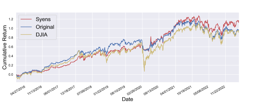
Figure 3. Cumulative return curves of different methods under the cash trading setting. (The results are averaged over 3 random seeds.)

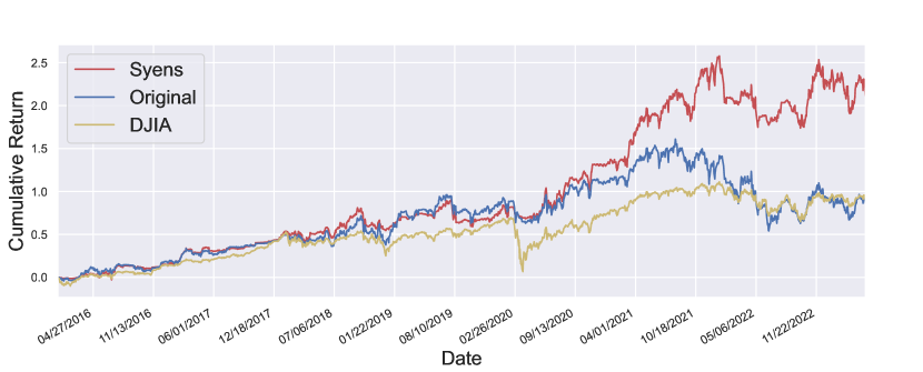
Figure 4. Cumulative return curves of different methods under the margin trading setting. (The results are averaged over 3 random seeds.)

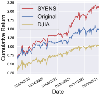
Figure 5. Cumulative return curves of different methods during a bull market period.

4.3. Ablation Study

In this section, we further conduct an ablation study to demonstrate the usefulness of the high-level programmatic strategy. Specifically, we remove all the logical conditions within the high-level program and the strategy becomes a simple bagging-based ensemble model with three tunable ensemble coefficients. We follow the same optimization method and setting as SYENS for this model. The results under the cash trading and margin trading scenarios are shown in Table 1 (denoted as SYENS w/o logic). Concretely, the results of SYENS w/o logic are significantly worse than SYENS. Under the margin trading setting, SYENS achieves $211.6\%$ in terms of cumulative return and $-24.5\%$ in terms of maximum drawdown, while SYENS w/o logic only achieves $142.4\%$ in terms of cumulative return and $-32.5\%$ in terms of maximum drawdown. And under the cash trading setting, SYENS achieves $111.4\%$ in terms of cumulative return, $-19.6\%$ in term of maximum drawdown, while SYENS w/o logic only achieves $88.7\%$ in terms of cumulative return and $-25.6\%$ in terms of maximum drawdown, which is even worse than the original ensemble model ($92.5\%$ in terms of cumulative return and $-21.8\%$ in terms of maximum drawdown). The ablation results demonstrate the effectiveness of the high-level programmatic strategy, which enables the SYENS model behavior to be more structured and robust.

Table 2. The comparative results of SYENS and baselines during the bull market and bear market periods.

Measurements	Bull Market			Bear Market
	DJIA	Original	SYENS (Ours)	DJIA	Original	SYENS (Ours)
Annual Return	32.5%	32.3% ± 10.2%	55.7% ± 4.3%	-41.9%	-26.3% ± 5.8%	-7.9% ± 3.0%
Cumulative Return	45.4%	45.2% ± 14.9%	80.1% ± 6.6%	-17.3%	-10.1% ± 2.5%	-2.8% ± 1.1%
Annual Volatility	16.8%	24.0% ± 5.7%	24.6% ± 3.3%	55.8%	25.1% ± 5.8%	18.2% ± 1.1%
Max Drawdown	-9.3%	-13.0% ± 4.7%	-14.9% ± 2.1%	-37.1%	-15.9% ± 3.8%	-9.3% ± 0.9%
Sharpe Ratio	1.768	1.277 ± 0.119	1.938 ± 0.104	-0.706	-1.1497 ± 0.407	-0.363 ± 0.15

4.4. Market Trend Analysis

To better understand the source of improvement, we further conduct an in-depth analysis of the model’s performance under different market trends. Concretely, we select two representative stock market periods, Figure 5 shows a bull market period (from 05/08/2020 to 09/03/2021) during which the cumulative return of DJIA is steadily increased, and Figure 6 shows a bear market period (stock market crash) (from 01/02/2020 to 05/07/2020) during which the cumulative return of DJIA is significantly decreased. It is obvious that SYENS is effective in improving over the baselines for both market trends. The detailed results are illustrated in Table 2. Specifically, during the bull market period, SYENS achieves a cumulative return of $80.1\%$, which is $+34.7\%$ higher than DJIA, while it also manages to balance the risk by achieving similarly low maximum drawdown $-14.9\%$. Regarding the bear market period, we observe that our model is more robust when dealing with market crashes. SYENS learns to cut losses more timely and achieves a much lower cumulative return loss $-2.8\%$ and maximum drawdown $-9.3\%$ compared to the DJIA ($-17.30\%$ in terms of cumulative return and $-37.10\%$ in terms of maximum drawdown) and the original ensemble model ($-10.1\%$ in terms of cumulative return and $-15.9\%$ in terms of maximum drawdown). The results indicate that the SYENS model manages to achieve much higher profit during the bull market period, and it has a stronger ability at handling market crashes and avoiding risk during the bear market period. These improvements can be attributed to the structured, logical design of its framework.

5. Related Work

5.1. DRL for Finance

The financial markets’ dynamic nature and increasing volatility have exposed the limitations of traditional trading strategies, including autoregressive moving average(ARMA) (Said and Dickey, 1984), pair trading (Elliott et al., 2005), etc. To tackle this challenge, the quantitative trading community is increasingly interested in utilizing deep learning and reinforcement learning techniques (Sutton et al., 1998; Wang et al., 2019), which have already achieved great performance in tackling complex stock trading (Wu et al., 2020; Lim et al., 2019), order execution (Yu et al., 2020; Breiman, 1996), market making (Zhao and Linetsky, 2021; Beysolow II and Beysolow II, 2019), and portfolio management (PM) (Hu and Lin, 2019; Wang et al., 2021b, a). Inspired by the accomplishment of critic-only reinforcement learning, which aims to tackle discrete action state representation and feature pattern recognition problems (Chen and Gao, 2019a; Zhang et al., 2020; Deng et al., 2016), previous works utilize DQN and its variations (e.g., DRQN) to design profitable trading strategies (Chen and Gao, 2019b). Besides, Li et al. propose a deep reinforcement learning (DRL) based PM framework (LSRECAAN) to perform online portfolio management in high-frequency trading with a relatively low turnover rate and quadratic dependency limitation (Li et al., 2023). Duan et al. propose the first end-to-end deep reinforcement learning method that adopts a probabilistic dynamic programming algorithm to explore a solution in the whole graph (Duan et al., 2022). To reduce variance and better optimization performance(Pricope, 2021), Jiang et al. introduce using the twin delayed deep deterministic policy gradient algorithm (TD3) to do risk management in stock trading (Jiang and Wang, 2022). Soleymani et al. propose a framework for PM that consists of a restricted stacked auto-encoder and convolutional neural network (Soleymani and Paquet, 2020).

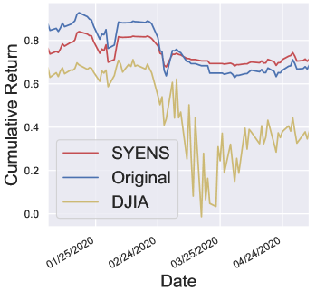
Figure 6. Cumulative return curves of different methods during a bear market period.

5.2. Program Synthesis by Sketching

For many real-world problems, the program search space is intractable, which poses a great challenge for the synthesis model. Sketching (Solar-Lezama, 2008; Singh et al., 2013) is a novel program synthesis paradigm that proposes combining the human expert and the program synthesizer by embedding domain expert knowledge as general program sketches (i.e., a program with hole). Then based on the program sketch, the synthesis is conducted to fill the hole. In this way, the candidate program search space can be greatly reduced. Singh et al. (Singh et al., 2013) propose a feedback generation system that automatically synthesizes program correction based on a general program sketch. Nye et al. (Nye et al., 2019) propose a two-stage neural program synthesis framework that first generates a coarse program sketch using a neural model, then leverages symbolic search for second-stage fine-tuning based on the generated sketch. Cao et al. propose a novel hybrid sketch-based programming language that combines the imperative and declarative programming paradigms and they use a program synthesis method based on differentiable ILP to generate programs with generalizable cause-effect logic for tasks that require navigation and multistep logical reasoning to accomplish.

5.3. Relational Inductive Bias

Incorporating human expert prior knowledge as relational inductive biases in neural network architectures has been proven effective in boosting models’ reasoning abilities. For example, the relational inductive bias of graph networks can improve the generalization and sample efficiency (Battaglia et al., 2018). Zhou et al. (Zhou et al., 2019) propose incorporating security expert knowledge in the form of abstract syntax tree, control flow graph, data flow graph etc. They embed these graphs with the graph neural networks which perform well in the vulnerability detection task. Architectural inductive bias can also be effective for an agent to learn relations within the domain of reinforcement learning (Zambaldi et al., 2018). Furthermore, the architectural inductive bias can also help improve the reasoning ability of the neural program synthesizers (Dong et al., [n. d.]) by achieving better generalization on the relational reasoning tasks and the decision-making tasks.

6. Conclusions

In this paper, we propose a novel logic-guided trading framework, called SYENS. Our proposed framework introduce utilizing the program synthesis by sketching paradigm. It is able to generate a hierarchical, programmatic ensemble strategy that synergistically combines multiple subpolicies with explicit logical conditions. Experimental results under both the cash trading and margin trading settings validate that our method is more robust, it can significantly outperform the state-of-the-art ensemble strategy as well as the Dow Jones Industrial Average by achieving much higher cumulative return and lower maximum drawdown. For future work, we plan to apply SYENS on other different market environments, e.g., option market, cryptocurrency market, etc. to further demonstrate the effectiveness of our framework. It would also be interesting to explore more sophisticated program sketches and more powerful program synthesis techniques to further improve the model’s robustness for the stock trading task.

References

- (1)
- Battaglia et al. (2018) Peter W Battaglia, Jessica B Hamrick, Victor Bapst, Alvaro Sanchez-Gonzalez, Vinicius Zambaldi, Mateusz Malinowski, Andrea Tacchetti, David Raposo, Adam Santoro, Ryan Faulkner, et al. 2018. Relational inductive biases, deep learning, and graph networks. arXiv preprint arXiv:1806.01261 (2018).
- Beysolow II and Beysolow II (2019) Taweh Beysolow II and Taweh Beysolow II. 2019. Market making via reinforcement learning. Applied Reinforcement Learning with Python: With OpenAI Gym, Tensorflow, and Keras (2019), 77–94.
- Breiman (1996) Leo Breiman. 1996. Bagging predictors. Machine learning 24 (1996), 123–140.
- Cao et al. (2021) Yushi Cao, Yan Zheng, Shang-Wei Lin, Yang Liu, Yon Shin Teo, Yuxuan Toh, and Vinay Vishnumurthy Adiga. 2021. Automatic HMI Structure Exploration Via Curiosity-Based Reinforcement Learning. In 2021 36th IEEE/ACM International Conference on Automated Software Engineering (ASE). IEEE, 1151–1155.
- Chen and Gao (2019a) Lin Chen and Qiang Gao. 2019a. Application of Deep Reinforcement Learning on Automated Stock Trading. In 2019 IEEE 10th International Conference on Software Engineering and Service Science (ICSESS). 29–33. https://doi.org/10.1109/ICSESS47205.2019.9040728
- Chen and Gao (2019b) Lin Chen and Qiang Gao. 2019b. Application of deep reinforcement learning on automated stock trading. In 2019 IEEE 10th International Conference on Software Engineering and Service Science (ICSESS). IEEE, 29–33.
- Chen et al. (2021) Xinyue Chen, Che Wang, Zijian Zhou, and Keith Ross. 2021. Randomized ensembled double q-learning: Learning fast without a model. arXiv preprint arXiv:2101.05982 (2021).
- Cui et al. (2023) Tianxiang Cui, Shusheng Ding, Huan Jin, and Yongmin Zhang. 2023. Portfolio constructions in cryptocurrency market: A CVaR-based deep reinforcement learning approach. Economic Modelling 119 (2023), 106078.
- Deng et al. (2016) Yue Deng, Feng Bao, Youyong Kong, Zhiquan Ren, and Qionghai Dai. 2016. Deep direct reinforcement learning for financial signal representation and trading. IEEE transactions on neural networks and learning systems 28, 3 (2016), 653–664.
- Dong et al. ([n. d.]) Honghua Dong, Jiayuan Mao, Tian Lin, Chong Wang, Lihong Li, and Denny Zhou. [n. d.]. Neural Logic Machines. In International Conference on Learning Representations.
- Duan et al. (2022) Zhongjie Duan, Cen Chen, Dawei Cheng, Yuqi Liang, and Weining Qian. 2022. Optimal Action Space Search: An Effective Deep Reinforcement Learning Method for Algorithmic Trading. In Proceedings of the 31st ACM International Conference on Information & Knowledge Management. 406–415.
- Ee et al. (2020) Yeo Keat Ee, Nurfadhlina Mohd Sharef, Razali Yaakob, and Khairul Azhar Kasmiran. 2020. LSTM based recurrent enhancement of DQN for stock trading. In 2020 IEEE Conference on Big Data and Analytics (ICBDA). IEEE, 38–44.
- Elliott et al. (2005) Robert J Elliott, John Van Der Hoek*, and William P Malcolm. 2005. Pairs trading. Quantitative Finance 5, 3 (2005), 271–276.
- Faußer and Schwenker (2011) Stefan Faußer and Friedhelm Schwenker. 2011. Ensemble methods for reinforcement learning with function approximation. In Multiple Classifier Systems: 10th International Workshop, MCS 2011, Naples, Italy, June 15-17, 2011. Proceedings 10. Springer, 56–65.
- Guan and Liu (2021) Mao Guan and Xiao-Yang Liu. 2021. Explainable deep reinforcement learning for portfolio management: an empirical approach. In Proceedings of the Second ACM International Conference on AI in Finance. 1–9.
- Hu and Lin (2019) Yuh-Jong Hu and Shang-Jen Lin. 2019. Deep reinforcement learning for optimizing finance portfolio management. In 2019 Amity International Conference on Artificial Intelligence (AICAI). IEEE, 14–20.
- Huang et al. (2019) Justin Huang, Dieter Fox, and Maya Cakmak. 2019. Synthesizing robot manipulation programs from a single observed human demonstration. In 2019 IEEE/RSJ International Conference on Intelligent Robots and Systems (IROS). IEEE, 4585–4592.
- Jiang and Wang (2022) Caiyu Jiang and Jianhua Wang. 2022. A Portfolio Model with Risk Control Policy Based on Deep Reinforcement Learning. Mathematics 11, 1 (2022), 19.
- Li et al. (2023) Jiahao Li, Yong Zhang, Xingyu Yang, and Liangwei Chen. 2023. Online portfolio management via deep reinforcement learning with high-frequency data. Information Processing & Management 60, 3 (2023), 103247.
- Lillicrap et al. (2015) Timothy P Lillicrap, Jonathan J Hunt, Alexander Pritzel, Nicolas Heess, Tom Erez, Yuval Tassa, David Silver, and Daan Wierstra. 2015. Continuous control with deep reinforcement learning. arXiv preprint arXiv:1509.02971 (2015).
- Lim et al. (2019) Bryan Lim, Stefan Zohren, and Stephen Roberts. 2019. Enhancing time-series momentum strategies using deep neural networks. The Journal of Financial Data Science 1, 4 (2019), 19–38.
- Liu et al. (2022) Xiao-Yang Liu, Ziyi Xia, Jingyang Rui, Jiechao Gao, Hongyang Yang, Ming Zhu, Christina Wang, Zhaoran Wang, and Jian Guo. 2022. FinRL-Meta: Market environments and benchmarks for data-driven financial reinforcement learning. Advances in Neural Information Processing Systems 35 (2022), 1835–1849.
- Mnih et al. (2016) Volodymyr Mnih, Adria Puigdomenech Badia, Mehdi Mirza, Alex Graves, Timothy Lillicrap, Tim Harley, David Silver, and Koray Kavukcuoglu. 2016. Asynchronous methods for deep reinforcement learning. In International conference on machine learning. PMLR, 1928–1937.
- Nan et al. (2022) Abhishek Nan, Anandh Perumal, and Osmar R Zaiane. 2022. Sentiment and knowledge based algorithmic trading with deep reinforcement learning. In Database and Expert Systems Applications: 33rd International Conference, DEXA 2022, Vienna, Austria, August 22–24, 2022, Proceedings, Part I. Springer, 167–180.
- Nye et al. (2019) Maxwell Nye, Luke Hewitt, Joshua Tenenbaum, and Armando Solar-Lezama. 2019. Learning to infer program sketches. In International Conference on Machine Learning. PMLR, 4861–4870.
- Polydoros and Nalpantidis (2017) Athanasios S Polydoros and Lazaros Nalpantidis. 2017. Survey of model-based reinforcement learning: Applications on robotics. Journal of Intelligent & Robotic Systems 86, 2 (2017), 153–173.
- Pricope (2021) Tidor-Vlad Pricope. 2021. Deep Reinforcement Learning in Quantitative Algorithmic Trading: A Review. arXiv:2106.00123 [cs.LG]
- Said and Dickey (1984) Said E Said and David A Dickey. 1984. Testing for unit roots in autoregressive-moving average models of unknown order. Biometrika 71, 3 (1984), 599–607.
- Schapire (2003) Robert E Schapire. 2003. The boosting approach to machine learning: An overview. Nonlinear estimation and classification (2003), 149–171.
- Schulman et al. (2017) John Schulman, Filip Wolski, Prafulla Dhariwal, Alec Radford, and Oleg Klimov. 2017. Proximal policy optimization algorithms. arXiv preprint arXiv:1707.06347 (2017).
- Sharpe (1998) William F Sharpe. 1998. The sharpe ratio. Streetwise–the Best of the Journal of Portfolio Management 3 (1998), 169–185.
- Singh et al. (2013) Rishabh Singh, Sumit Gulwani, and Armando Solar-Lezama. 2013. Automated feedback generation for introductory programming assignments. In Proceedings of the 34th ACM SIGPLAN conference on Programming language design and implementation. 15–26.
- Solar-Lezama (2008) Armando Solar-Lezama. 2008. Program synthesis by sketching. University of California, Berkeley.
- Soleymani and Paquet (2020) Farzan Soleymani and Eric Paquet. 2020. Financial portfolio optimization with online deep reinforcement learning and restricted stacked autoencoder—DeepBreath. Expert Systems with Applications 156 (2020), 113456.
- Sutton and Barto (2018) Richard S Sutton and Andrew G Barto. 2018. Reinforcement learning: An introduction. MIT press.
- Sutton et al. (1998) Richard S Sutton, Andrew G Barto, et al. 1998. Introduction to reinforcement learning. Vol. 135. MIT press Cambridge.
- Wang et al. (2019) Jingyuan Wang, Yang Zhang, Ke Tang, Junjie Wu, and Zhang Xiong. 2019. Alphastock: A buying-winners-and-selling-losers investment strategy using interpretable deep reinforcement attention networks. In Proceedings of the 25th ACM SIGKDD international conference on knowledge discovery & data mining. 1900–1908.
- Wang et al. (2021b) Rundong Wang, Hongxin Wei, Bo An, Zhouyan Feng, and Jun Yao. 2021b. Commission fee is not enough: A hierarchical reinforced framework for portfolio management. In Proceedings of the AAAI Conference on Artificial Intelligence, Vol. 35. 626–633.
- Wang et al. (2021a) Zhicheng Wang, Biwei Huang, Shikui Tu, Kun Zhang, and Lei Xu. 2021a. DeepTrader: a deep reinforcement learning approach for risk-return balanced portfolio management with market conditions Embedding. In Proceedings of the AAAI Conference on Artificial Intelligence, Vol. 35. 643–650.
- Wolpert (1992) David H Wolpert. 1992. Stacked generalization. Neural networks 5, 2 (1992), 241–259.
- Wu et al. (2020) Xing Wu, Haolei Chen, Jianjia Wang, Luigi Troiano, Vincenzo Loia, and Hamido Fujita. 2020. Adaptive stock trading strategies with deep reinforcement learning methods. Inf. Sci. 538 (2020), 142–158.
- Yang et al. (2020) Hongyang Yang, Xiao-Yang Liu, Shan Zhong, and Anwar Walid. 2020. Deep reinforcement learning for automated stock trading: An ensemble strategy. In Proceedings of the first ACM international conference on AI in finance. 1–8.
- Yu et al. (2020) Xiang Yu, Guoliang Li, Chengliang Chai, and Nan Tang. 2020. Reinforcement learning with tree-lstm for join order selection. In 2020 IEEE 36th International Conference on Data Engineering (ICDE). IEEE, 1297–1308.
- Zambaldi et al. (2018) Vinicius Zambaldi, David Raposo, Adam Santoro, Victor Bapst, Yujia Li, Igor Babuschkin, Karl Tuyls, David Reichert, Timothy Lillicrap, Edward Lockhart, et al. 2018. Relational deep reinforcement learning. arXiv preprint arXiv:1806.01830 (2018).
- Zhang et al. (2020) Zihao Zhang, Stefan Zohren, and Stephen Roberts. 2020. Deep reinforcement learning for trading. The Journal of Financial Data Science 2, 2 (2020), 25–40.
- Zhao and Linetsky (2021) Muchen Zhao and Vadim Linetsky. 2021. High frequency automated market making algorithms with adverse selection risk control via reinforcement learning. In Proceedings of the Second ACM International Conference on AI in Finance. 1–9.
- Zheng et al. (2021) Yan Zheng, Yi Liu, Xiaofei Xie, Yepang Liu, Lei Ma, Jianye Hao, and Yang Liu. 2021. Automatic web testing using curiosity-driven reinforcement learning. In 2021 IEEE/ACM 43rd International Conference on Software Engineering (ICSE). IEEE, 423–435.
- Zheng et al. (2019) Yan Zheng, Xiaofei Xie, Ting Su, Lei Ma, Jianye Hao, Zhaopeng Meng, Yang Liu, Ruimin Shen, Yingfeng Chen, and Changjie Fan. 2019. Wuji: Automatic online combat game testing using evolutionary deep reinforcement learning. In 2019 34th IEEE/ACM International Conference on Automated Software Engineering (ASE). IEEE, 772–784.
- Zhou et al. (2019) Yaqin Zhou, Shangqing Liu, Jingkai Siow, Xiaoning Du, and Yang Liu. 2019. Devign: Effective vulnerability identification by learning comprehensive program semantics via graph neural networks. Advances in neural information processing systems 32 (2019).