Cokrig-and-Regress for Spatially Misaligned Environmental Data

Abstract

Spatially misaligned data, where the response and covariates are observed at different spatial locations, commonly arise in many environmental studies. Much of the statistical literature on handling spatially misaligned data has been devoted to the case of a single covariate and a linear relationship between the response and this covariate. Motivated by spatially misaligned data collected on air pollution and weather in China, we propose a cokrig-and-regress (CNR) method to estimate spatial regression models involving multiple covariates and potentially non-linear associations. The CNR estimator is constructed by replacing the unobserved covariates (at the response locations) by their cokriging predictor derived from the observed but misaligned covariates under a multivariate Gaussian assumption, where a generalized Kronecker product covariance is used to account for spatial correlations within and between covariates. A parametric bootstrap approach is employed to bias-correct the CNR estimates of the spatial covariance parameters and for uncertainty quantification. Simulation studies demonstrate that CNR outperforms several existing methods for handling spatially misaligned data, such as nearest-neighbor interpolation. Applying CNR to the spatially misaligned air pollution and weather data in China reveals a number of non-linear relationships between $\text{PM}_{2.5}$ concentration and several meteorological covariates.

Keywords: Cokriging, Generalized Kronecker product, Matérn covariance, Parametric bootstrap, Spatial regression

1 Introduction

Spatial regression models are commonly used to study the relationship between a response and one or more covariates while accounting for potential (residual) spatial correlation between the responses (Cressie and Wikle,, 2015), with applications in ecology, epidemiology, and environmental studies among many fields. Much of the current literature on spatial regression modeling assumes the response and the covariates are observed at the same spatial location. However, improving technologies means it is becoming increasingly common for the response and covariates to come from different data sources. One issue that can arise as a result of this is spatial misalignment between the response and the covariates (Jhun et al.,, 2015; Liu et al.,, 2020; Greenstone et al.,, 2022) i.e., the response and the covariates are observed at two different sets of spatial locations. As a motivating example, we consider environmental data collected on pollutant concentration (response) and meteorological variables (covariates) in China, where the pollution monitoring stations have different spatial locations to the weather stations.

In environmental science, the most common approach for overcoming spatial misalignment is based on nearest-neighbor interpolation, where the unobserved meteorological covariates at each pollution station are predicted to be the same as those observed at the closest meteorological station (e.g., Jhun et al.,, 2015; Greenstone et al.,, 2022). In related works, Reich et al., (2011) and Liu et al., (2020) predicted each meteorological covariate separately using kriging techniques to construct spatially aligned datasets. These studies do not focus on the spatial misalignment problem per-se, and so they treat the predicted/interpolated covariates as fixed when conducting inference. Ignoring this prediction uncertainty however risks underestimating the variability of the model parameter estimates. A more systematic approach to handling spatially misaligned data is the krige-and-regress (KNR) method of Madsen et al., (2008), who also used kriging to spatially align the covariate to the response, but developed a Monte Carlo method to estimate the variance of the regression coefficient estimator which takes into account additional variability due to the predicted covariate. Szpiro et al., (2011) further developed KNR and proposed three parametric bootstrap techniques to obtain the corrected variance estimator of the regression coefficient estimator, based on framing the uncertainty in the predicted covariate as a form of measurement error. More recently, Pouliot, (2023) studied a bootstrap approach for KNR but under a survey sampling framework. In all of these papers on KNR, only a single misaligned covariate was considered, along with a linear response-covariate relationship. These assumptions can be too restrictive in practice though, as many environmental studies involve multiple misaligned and correlated covariates, and potentially non-linear associations between the response and the covariates; see the motivating pollution study in China in Section 5 for instance.

In this article, to overcome the above issues we propose a new cokrig-and-regress (CNR) method for spatially misaligned data with multiple correlated covariates. Building upon Madsen et al., (2008), the CNR method employs a cokriging predictor (Stein and Corsten,, 1991) of the unobserved covariates at the response locations.In particular, to utilize the spatial information both within the same covariate and between covariates, we assume the joint vector of all covariates at the response and covariate locations follows a multivariate Gaussian distribution with a covariance matrix constructed based on a generalized Kronecker product form (Martinez-Beneito,, 2013; Bonat et al.,, 2021). This induces cross-correlations between covariates in such a way that it preserves the marginal covariance matrix of each covariate. In our setting of multiple spatial covariates, we use the Matérn class of correlation functions (Matérn,, 1960) to model the marginal spatial correlation, while the cross-correlation matrix between covariates is left unstructured. The predicted covariates obtained from cokriging are used in place of the unobserved covariates in a spatial linear mixed model for the response, where we include a spatial random effect whose covariance is (again) characterized by a Matérn correlation function. To account for potentially non-linear functions of the covariates, we allow polynomial or spline basis functions for one or more of the covariates in the spatial linear mixed model. For uncertainty quantification, we follow the ideas of Szpiro et al., (2011) and Pouliot, (2023) and develop a parametric bootstrap approach to construct confidence intervals/bands for the regression coefficients/smoothing functions in CNR. We also use the parametric bootstrap to bias-correct the spatial covariance parameter estimates in the spatial linear mixed model, which turns out to play an important role in improving the inferential performance of the CNR method.

Simulation studies show CNR performs well in recovering the underlying response-covariate relationship when data are spatially misaligned, while existing approaches such as nearest-neighbor interpolation can suffer from substantial biases. The parametric bootstrap is also shown to be effective in producing confidence intervals with empirical coverage probability close to the nominal level, greatly outperforming naive variance estimators that ignore the uncertainty in correcting for the spatial misalignment, as well as a variance estimator that ignores the spatial cross-correlation between covariates. Applying CNR to the spatially misaligned air pollution and meteorological data from China, we find evidence of complex non-linear associations between $\text{PM}_{2.5}$ concentration and meteorological covariates such as temperature and precipitation, while the resulting spatial maps constructed from cokriging agree with scientific explanations for the spatial distribution of these meteorological covariates in China. The confidence bands for the estimated smoothing functions of the covariates using the parametric bootstrap approach are always wider than those using the naive variance estimator, which is similar to the findings from our simulation studies where the naive variance estimator underestimates the uncertainty of the CNR estimator.

The rest of this article is organized as follows. Section 2 introduces the model for the spatial misalignment problem and the generalized Kronecker product covariance matrix. Section 3 develops the CNR method and the parametric bootstrap procedure. Simulation studies are given in Section 4, while an application to spatially misaligned air pollution and meteorological data from China is provided in Section 5. Section 6 offers some concluding remarks.

2 Data and Model Set-Up

Let $S=\{s_{1},\cdots,s_{N}\}\subset D$ denote a set of spatial locations in some domain of interest $D$, and suppose $\bm{y}=(y_{1},\cdots,y_{N})^{\top}=\left(y(s_{1}),\cdots,y(s_{N})\right)^{\top}$ is an $N$-vector of responses observed at locations in $S$. In addition to the response, consider a set of $K$ covariates where $\bm{x}_{k}=(x_{1k},\cdots,x_{Nk})^{\top}=(x_{k}(s_{1}),\cdots,x_{k}(s_{N}))^{\top}$ denotes the set of values for the $k$-th covariate at locations in $S$ for $k=1,\cdots,K$. We assume the response follows the spatial linear mixed model

$$y_{i}=\beta_{0}+\sum_{k=1}^{K}\bm{f}_{k}(x_{ik})^{\top}\bm{\beta}_{k}+\rho_{i}+\epsilon_{i},\text{ for }i=1,\cdots,N,$$ (1)

where $\beta_{0}$ is an intercept term, $\bm{f}_{k}(x_{ik})$ is a known vector-valued function evaluated at $x_{ik}$ for $k=1,\cdots,K$, and $\bm{\beta}_{k}$ denotes the corresponding regression coefficients. Equation (1) includes the special case of $\bm{f}_{k}(x_{ik})^{\top}\bm{\beta}_{k}=x_{ik}\beta_{k}$ and $K=1$; such a model is the focus for much statistical research on spatially misaligned data, including the KNR method of Madsen et al., (2008). In this article however, we focus on a more general setting with $K>1$ and potentially non-linear response-covariate relationships as modeled through the vector-valued function $\bm{f}_{k}(x_{ik})$. For instance, in the motivating air pollution data in China, we have $K=7$ meteorological covariates and consider second order polynomial or natural cubic spline basis functions, as part of $\bm{f}_{k}(x_{ik})$. Finally, $\bm{\rho}=(\rho_{1},\cdots,\rho_{N})^{\top}=(\rho(s_{1}),\cdots,\rho(s_{N}))^{\top}$ is a vector of spatial random effects which we assume follows a multivariate Gaussian distribution with mean zero and spatial covariance matrix $\bm{\Sigma}_{\rho}$, while $\bm{\epsilon}=(\epsilon_{1},\cdots,\epsilon_{N})^{\top}=(\epsilon(s_{1}),\cdots,\epsilon(s_{N}))^{\top}$ is a vector of independent and identically distributed (i.i.d) residuals assumed to be normally distributed with mean zero and variance $\tau_{\epsilon}>0$. The covariance matrix $\bm{\Sigma}_{\rho}$ captures the residual spatial correlation in the spatial linear mixed model, and we discuss its form shortly.

In the setting of spatially misaligned data, the response and covariates are not observed at the same spatial locations. We formalize this as follows. Assume at locations in $S$ only the response vector $\bm{y}$ is observed, while the covariates $\bm{x}_{k}$ are missing for $k=1,\cdots,K$. Let $\tilde{S}=\{\tilde{s}_{1},\cdots,\tilde{s}_{M}\}\subset D$ denote another set of spatial locations such that $S\cap\tilde{S}=\emptyset$, where we record $\tilde{\bm{x}}_{k}=(\tilde{x}_{1k},\cdots,\tilde{x}_{Mk})^{\top}=(x_{k}(\tilde{s}_{1}),\cdots,x_{k}(\tilde{s}_{M}))^{\top}$ as covariate values for $k=1,\cdots,K$. We aim to estimate and perform inference on the coefficients $\bm{\beta}_{k}$, and functions thereof, in equation (1), when the responses and the covariates are spatially misaligned as described above.

To overcome spatial misalignment, we begin by first specifying a model for each covariate at all spatial locations i.e., $(\tilde{\bm{x}}_{k}^{\top},\bm{x}_{k}^{\top})^{\top}$. Specifically, for $k=1,\cdots,K$, we assume $(\tilde{\bm{x}}_{k}^{\top},\bm{x}_{k}^{\top})^{\top}$ follows a multivariate Gaussian distribution with mean vector $\mu_{k}\bm{1}_{M+N}$ and covariance matrix

$$\bm{\Sigma}_{k}=\begin{pmatrix}\bm{\Sigma}_{k,\tilde{S}}&\bm{\Sigma}_{k,\tilde{S}S}\\ \bm{\Sigma}_{k,S\tilde{S}}&\bm{\Sigma}_{k,S}\end{pmatrix}=\begin{pmatrix}\mathrm{Cov}(\tilde{\bm{x}}_{k},\tilde{\bm{x}}_{k})&\mathrm{Cov}(\tilde{\bm{x}}_{k},\bm{x}_{k})\\ \mathrm{Cov}(\bm{x}_{k},\tilde{\bm{x}}_{k})&\mathrm{Cov}(\bm{x}_{k},\bm{x}_{k})\end{pmatrix},$$

where $\bm{1}_{M+N}$ is an $(M+N)$-vector of ones, $\mathrm{Cov}(x_{k}(s),x_{k}(s^{\prime}))=\sigma_{k}^{2}\mathcal{M}(\|s-s^{\prime}\|;\nu_{k},\alpha_{k})+\tau_{k}1_{\{s=s^{\prime}\}}$ for $s,s^{\prime}\in D$ and $\|s-s^{\prime}\|$ denotes a distance measure between the two locations $s$ and $s^{\prime}$. Here we choose $\mathcal{M}(d;\nu,\alpha)=2^{1-\nu}(\alpha d)^{\nu}K_{\nu}(\alpha d)/\Gamma(\nu)$ to be the Matérn class of correlation functions with smoothness $\nu>0$ and range $\alpha>0$ parameters, where $K_{\nu}(\cdot)$ is the modified Bessel function of order $\nu$, and $\Gamma(\cdot)$ is the Gamma function. The quantity $\sigma^{2}>0$ denotes the Matérn variance, while a nugget effect is included such that $1_{\{\cdot\}}$ denotes the indicator function and $\tau>0$ denotes the nugget parameter.

Returning to the spatial linear mixed model in (1), we also use a Matérn correlation function to characterize the spatial covariance matrix of the spatial random effects i.e., the elements of $\bm{\Sigma}_{\rho}$ are such that $\mathrm{Cov}\{\rho(s),\rho(s^{\prime})\}=\sigma^{2}_{\rho}\mathcal{M}(\|s-s^{\prime}\|;\nu_{\rho},\alpha_{\rho})$. The Matérn correlation function is a well-established and widely used method for characterizing the spatial correlation structure in spatial regression models (Lindgren and Rue,, 2015), with special cases being the exponential correlation function when $\nu=1/2$, and the squared exponential or Gaussian correlation function when $\nu\to\infty$. In practice it is quite common to fix the spatial smoothness parameter $\nu$ while estimating the variance $\sigma^{2}$ and spatial range $\alpha$ (e.g., Lindgren and Rue,, 2015; Bakka et al.,, 2018, who fixed $\nu=1$ for two-dimensional spatial data with an Euclidean distance metric), and we adopt this approach for our spatial misalignment application while choosing $\nu$ based on exploratory data analysis.

2.1 Generalized Kronecker Product Covariance Matrix

So far, we have specified a model for spatial correlation within a covariate, which largely follows from the work of Madsen et al., (2008), Szpiro et al., (2011) and Pouliot, (2023) for spatial misalignment. However, as discussed in Section 1, when $K>1$ it is of interest to allow for the covariates to be correlated with each other. For example, we find evidence of moderate correlations between several of the meteorological covariates in our motivating air pollution data in Section 5. Accounting for such spatial cross-correlations should improve uncertainty quantification and hence inference on the $\bm{\beta}_{k}$’s in equation (1).

Let $\bm{x}=(\tilde{\bm{x}}_{1}^{\top},\bm{x}_{1}^{\top},\cdots,\tilde{\bm{x}}_{K}^{\top},\bm{x}_{K}^{\top})^{\top}$ denote the stacked $K(M+N)$-vector of $K$ covariates at locations in both $\tilde{S}$ and $S$, and $\bm{x}_{\tilde{S}}=(\tilde{\bm{x}}_{1}^{\top},\cdots,\tilde{\bm{x}}_{K}^{\top})^{\top}$ and $\bm{x}_{S}=(\bm{x}_{1}^{\top},\cdots,\bm{x}_{K}^{\top})^{\top}$ be the $KM$- and $KN$-vectors of covariates at locations in $\tilde{S}$ and $S$, respectively. Then we assume $\bm{x}$ follows a multivariate Gaussian distribution with mean vector $\bm{\mu}\otimes\bm{1}_{M+N}$ and covariance matrix

$$\bm{\Sigma}=\mathrm{Bdiag}(\bm{L}_{1},\cdots,\bm{L}_{K})(\bm{R}\otimes\bm{I}_{M+N})\mathrm{Bdiag}(\bm{L}_{1},\cdots,\bm{L}_{K})^{\top},$$ (2)

where $\bm{\mu}=(\mu_{1},\cdots,\mu_{K})^{\top}$, $\bm{R}$ is a $K\times K$ correlation matrix capturing the cross-correlation among the $K$ covariates, $\bm{I}_{M+N}$ is the $(M+N)\times(M+N)$ identity matrix, $\bm{L}_{k}$ is the lower Cholesky factor of $\bm{\Sigma}_{k}$, and $\mathrm{Bdiag}(\cdot)$ denotes the block diagonal matrix operator.

When $K=1$, it is easy to see that $\bm{\Sigma}$ in equation (2) reduces to a single Matérn covariance matrix $\bm{\Sigma}_{k}$ discussed in the previous section. For $K>1$, the covariance matrix in (2) has the generalized Kronecker product form proposed by Martinez-Beneito, (2013), and subsequently used by Bonat and Jørgensen, (2016); Bonat et al., (2021) among others for multivariate covariance generalized linear models. This form induces a relatively simple structure for the spatial cross-correlation between two covariates: $\mathrm{Cov}\{(\tilde{\bm{x}}_{k_{1}}^{\top},\bm{x}_{k_{1}}^{\top})^{\top},(\tilde{\bm{x}}_{k_{2}}^{\top},\bm{x}_{k_{2}}^{\top})^{\top}\}=r_{k_{1}k_{2}}\bm{L}_{k_{1}}\bm{L}_{k_{2}}^{\top}$ for $k_{1}\neq k_{2}$, where $r_{k_{1}k_{2}}$ is the $(k_{1},k_{2})$-th element of $\bm{R}$. Although such a simple form may be less flexible than other options for modeling spatial cross-covariances (see Salvana and Genton,, 2020, and references therein), the generalized Kronecker product does offer some notable advantages in terms of computation as well as the relatively smaller number of parameters needing to be estimated, as we shall see shortly.

The assumed model for the full vector $\bm{x}$ in (2) implies that the vector of only the observed covariates, $\bm{x}_{\tilde{S}}$, is multivariate Gaussian distributed with mean $\bm{\mu}\otimes\bm{1}_{M}$ and covariance matrix

$$\bm{\Sigma}_{\tilde{S}}=\mathrm{Bdiag}(\bm{L}_{1,\tilde{S}},\cdots,\bm{L}_{K,\tilde{S}})(\bm{R}\otimes\bm{I}_{M})\mathrm{Bdiag}(\bm{L}_{1,\tilde{S}},\cdots,\bm{L}_{K,\tilde{S}})^{\top}.$$ (3)

This is analogous to the form of $\bm{\Sigma}$ in (2), where $\bm{L}_{k,\tilde{S}}$ is the lower Cholesky factor of $\bm{\Sigma}_{k,\tilde{S}}$.

Let $\bm{\theta}_{x}=(\bm{\mu}^{\top},\sigma_{1}^{2},\cdots,\sigma_{K}^{2},\nu_{1},\cdots,\nu_{K},\alpha_{1},\cdots,\alpha_{K},\tau_{1},\cdots,\tau_{K},\mathrm{vech}(\bm{R})^{\top})^{\top}$ be the $(5K+K(K+1)/2)$-vector of parameters characterizing the joint distribution of the covariates. The generalized Kronecker product form for $\bm{\Sigma}_{\tilde{S}}$ means that the parameters $\bm{\theta}_{x}$ can be estimated directly from the marginal distribution of just the observed covariate vector $\bm{x}_{\tilde{S}}$. Additionally, the precision matrix can be computed efficiently as $\bm{\Sigma}_{\tilde{S}}^{-1}=\mathrm{Bdiag}(\bm{L}_{1,\tilde{S}}^{-1},\cdots,\bm{L}_{K,\tilde{S}}^{-1})^{\top}(\bm{R}^{-1}\otimes\bm{I}_{M})\mathrm{Bdiag}(\bm{L}_{1,\tilde{S}}^{-1},\cdots,\bm{L}_{K,\tilde{S}}^{-1})$. This only requires inverting matrices of dimensions $M\times M$ and $K\times K$, as opposed to directly inverting a matrix of dimension $MK\times MK$.

3 Cokrig-and-Regress

We propose cokrig-and-regress (CNR) for estimating $\bm{\beta}=(\beta_{0},\bm{\beta}_{1}^{\top},\cdots,\bm{\beta}_{K}^{\top})^{\top}$ in equation (1) when only $\bm{y}$ and the misaligned $\bm{x}_{\tilde{S}}$ are observed. The proposed approach can be viewed as a generalization of KNR in Madsen et al., (2008) to allow for $K>1$ covariates and potentially non-linear associations between the response and the covariates, while taking into account potential spatial cross-correlations between covariates.

The CNR method consists of the following three steps. First, we estimate the parameters characterizing the distribution of the covariates i.e., $\bm{\theta}_{x}$. Let $\bm{\theta}_{x,k}=(\mu_{k},\sigma^{2}_{k},\nu_{k},\alpha_{k},\tau_{k})^{\top}$ be the parameters associated with the marginal distribution of the $k$-th covariate for $k=1,\cdots,K$. Then we begin by maximizing the marginal log-likelihood of $\tilde{\bm{x}}_{k}$ for $k=1,\cdots,K$,

$$\hat{\bm{\theta}}_{x,k} =\arg\max_{\bm{\theta}_{x,k}}\left\{-\frac{1}{2}\log\det(\bm{\Sigma}_{k,\tilde{S}})-\frac{1}{2}(\tilde{\bm{x}}_{k}-\mu_{k}\bm{1}_{M})^{\top}\bm{\Sigma}_{k,\tilde{S}}^{-1}(\tilde{\bm{x}}_{k}-\mu_{k}\bm{1}_{M})\right\},$$ (4)

where $\bm{\Sigma}_{k,\tilde{S}}$ is parameterized by $(\sigma^{2}_{k},\nu_{k},\alpha_{k},\tau_{k})^{\top}$ and constants in the log-likelihood with respect to the parameters are omitted. In Section LABEL:sec:appendix_unbiased_estimating of the supplementary material, we show that this approach results in asymptotically unbiased estimates of $\hat{\bm{\theta}}_{x,k}$ when the covariates are truly cross-correlated. Recalling that $\bm{\Sigma}_{k,\tilde{S}}$ takes the form of a Matérn covariance matrix for $k=1,\cdots,K$, equation (4) can be straightforwardly solved e.g., using the R package spaMM (Rousset and Ferdy,, 2014), where $\nu_{k}$ is assumed to be chosen based on exploratory data analysis and then fixed throughout. Next, let $\hat{\bm{\Sigma}}_{k,\tilde{S}}$ denote the estimated marginal covariance matrix of $\tilde{\bm{x}}_{k}$ evaluated at $\hat{\bm{\theta}}_{x,k}$, and $\hat{\bm{L}}_{k,\tilde{S}}$ be the corresponding Cholesky factor for $k=1,\cdots,K$. Writing $\hat{\bm{\Sigma}}_{\tilde{S}}(\bm{R})=\mathrm{Bdiag}(\hat{\bm{L}}_{1,\tilde{S}},\cdots,\hat{\bm{L}}_{K,\tilde{S}})(\bm{R}\otimes\bm{I}_{M})\mathrm{Bdiag}(\hat{\bm{L}}_{1,\tilde{S}},\cdots,\hat{\bm{L}}_{K,\tilde{S}})^{\top}$ and given $\hat{\bm{\theta}}_{x,k}$ for $k=1,\cdots,K$, then we can construct a one-step estimator for $\bm{R}$ as

$$\hat{\bm{R}} =\arg\max_{\bm{R}}\left\{-\frac{1}{2}\log\left|\hat{\bm{\Sigma}}_{\tilde{S}}(\bm{R})\right|-\frac{1}{2}(\bm{x}_{\tilde{S}}-\hat{\bm{\mu}}\otimes\bm{1}_{M})^{\top}\hat{\bm{\Sigma}}_{\tilde{S}}(\bm{R})^{-1}(\bm{x}_{\tilde{S}}-\hat{\bm{\mu}}\otimes\bm{1}_{M})\right\}$$

$$=\frac{1}{M}\begin{pmatrix}(\tilde{\bm{x}}_{1}^{\top}-\hat{\mu}_{1}\bm{1}_{M}^{\top})\hat{\bm{L}}_{1,\tilde{S}}^{-1\top}\\ \vdots\\ (\tilde{\bm{x}}_{K}^{\top}-\hat{\mu}_{K}\bm{1}_{M}^{\top})\hat{\bm{L}}_{K,\tilde{S}}^{-1\top}\end{pmatrix}\begin{pmatrix}\hat{\bm{L}}_{1,\tilde{S}}^{-1}(\tilde{\bm{x}}_{1}-\hat{\mu}_{1}\bm{1}_{M}),\cdots,\hat{\bm{L}}_{K,\tilde{S}}^{-1}(\tilde{\bm{x}}_{K}-\hat{\mu}_{K}\bm{1}_{M})\end{pmatrix},$$ (5)

where $\hat{\bm{\mu}}=(\hat{\mu}_{1},\cdots,\hat{\mu}_{K})^{\top}$ is the vector of estimated marginal mean parameters from (4); see Section LABEL:sec:appendix_unbiased_estimating of the supplementary material for further discussion on the one-step estimator. It is also worth noting that the aforementioned two-step estimation procedure for $\bm{\theta}_{x}$ is facilitated by the generalized Kronecker product form in (3).

In the second step of CNR, we predict the unobserved $\bm{x}_{S}$ i.e., at the spatial locations where only the response was recorded, based on the observed $\bm{x}_{\tilde{S}}$ and the estimates from the first step (denoted here as $\hat{\bm{\theta}}_{x}$). Given the assumption of multivariate normality, it is straightforward to obtain the prediction of $\bm{x}_{S}$ by cokriging i.e., the empirical best linear unbiased prediction of $\bm{x}_{S}$ given $\bm{x}_{\tilde{S}}$ which makes use of the spatial correlations both within and between covariates,

$$\hat{\bm{x}}_{S}=\mathrm{E}(\bm{x}_{S}|\bm{x}_{\tilde{S}};\hat{\bm{\theta}}_{x})=\hat{\bm{\mu}}\otimes\bm{1}_{N}+\hat{\bm{\Sigma}}_{S\tilde{S}}\hat{\bm{\Sigma}}_{\tilde{S}}^{-1}\left(\bm{x}_{\tilde{S}}-\hat{\bm{\mu}}\otimes\bm{1}_{M}\right),$$ (6)

where $\hat{\bm{\Sigma}}_{S\tilde{S}}$ and $\hat{\bm{\Sigma}}_{\tilde{S}}$ are the estimated cross-covariance matrix between $\bm{x}_{S}$ and $\bm{x}_{\tilde{S}}$ and the estimated covariance matrix of $\bm{x}_{\tilde{S}}$, respectively, based on extracting the relevant rows and columns of $\hat{\bm{\Sigma}}$ i.e., the estimate of $\bm{\Sigma}$ in equation (2) evaluated at $\hat{\bm{\theta}}_{x}$ and $\hat{\bm{R}}$. Again, with the generalized Kronecker product form this can be efficiently computed as we can straightforwardly show that the joint prediction of $K$ covariates based on cokriging using (6) is equivalent to computing the predictors $\hat{\bm{x}}_{S}=(\hat{\bm{x}}_{1}^{\top},\cdots,\hat{\bm{x}}_{K}^{\top})^{\top}$ with $\hat{\bm{x}}_{k}=(\hat{x}_{1k},\cdots,\hat{x}_{Nk})^{\top}=\hat{\mu}_{k}\bm{1}_{N}+\hat{\bm{\Sigma}}_{k,S\tilde{S}}\hat{\bm{\Sigma}}_{k,\tilde{S}}^{-1}(\tilde{\bm{x}}_{k}-\hat{\mu}_{k}\bm{1}_{M})$ where $\hat{\bm{\Sigma}}_{k,S\tilde{S}}$ denotes $\bm{\Sigma}_{k,S\tilde{S}}$ evaluated at $\hat{\bm{\theta}}_{x,k}$ for $k=1,\cdots,K$. This equivalence can be used to reduce computational effort as we only have to deal with matrices of dimension $M\times M$ and $M\times N$ instead of $MK\times MK$ and $MK\times NK$ when performing cokriging. It is worth highlighting that such equivalence does not undermine the use of (2) for modeling the correlation between the covariates: explicitly taking into account the spatial cross-correlations between covariates improves our uncertainty quantification when we develop our bootstrap approach later on in Section 3.1 for inference.

In the final step of CNR, we substitute the predicted $\hat{x}_{ik}$’s into equation (1) and maximize the log-likelihood of the spatial linear mixed model. Letting

$$\hat{\bm{B}}=\begin{pmatrix}1&\bm{f}_{1}(\hat{x}_{11})^{\top}&\cdots&\bm{f}_{K}(\hat{x}_{1K})^{\top}\\ \vdots&\vdots&\vdots&\vdots\\ 1&\bm{f}_{1}(\hat{x}_{n1})^{\top}&\cdots&\bm{f}_{K}(\hat{x}_{nK})^{\top}\\ \end{pmatrix},$$

then we compute the estimates

$$(\hat{\bm{\beta}}^{\top},\hat{\bm{\theta}}_{\rho}^{\top},\hat{\tau}_{\epsilon})^{\top} =\arg\max_{(\bm{\beta},\bm{\theta}_{\rho},\tau_{\epsilon})}\left\{-\frac{1}{2}\log\left|\bm{\Sigma}_{\rho}+\tau_{\epsilon}\bm{I}_{N}\right|-\frac{1}{2}(\bm{y}-\hat{\bm{B}}\bm{\beta})^{\top}(\bm{\Sigma}_{\rho}+\tau_{\epsilon}\bm{I}_{N})^{-1}(\bm{y}-\hat{\bm{B}}\bm{\beta})\right\},$$ (7)

where $\bm{\Sigma}_{\rho}$ is parameterized by $\bm{\theta}_{\rho}=(\sigma^{2}_{\rho},\nu_{\rho},\alpha_{\rho})^{\top}$. The regression coefficient estimators take the form of a generalized least squares estimator $\hat{\bm{\beta}}=\{\hat{\bm{B}}^{\top}(\hat{\bm{\Sigma}}_{\rho}+\hat{\tau}_{\epsilon}\bm{I}_{N})^{-1}\hat{\bm{B}}\}^{-1}\hat{\bm{B}}^{\top}(\hat{\bm{\Sigma}}_{\rho}+\hat{\tau}_{\epsilon}\bm{I}_{N})^{-1}\bm{y}$, where $\hat{\bm{\Sigma}}_{\rho}$ denotes the estimated covariance matrix evaluated at $\hat{\bm{\theta}}_{\rho}$. Since $\bm{\Sigma}_{\rho}$ has the form of a Matérn covariance matrix, then we adopt a similar approach to the estimation of $\hat{\bm{\theta}}_{x,k}$’s in (4) for estimating the parameters in (7).

As a final remark, when $\bm{f}_{k}(\cdot)^{\top}\bm{\beta}_{k}$ is used to model a non-linear relationship between the response and the $k$-th covariate, then for interpretation purposes we focus on the estimation and uncertainty quantification of the conditional smoothing function $\hat{\beta}_{0}+\bm{f}_{k}(x_{k})^{\top}\hat{\bm{\beta}}_{k}+\sum_{l\neq k}\bm{f}_{l}(c_{l})^{\top}\hat{\bm{\beta}}_{l}$, where we vary the value of $x_{k}$ while conditioning on the other covariates e.g., setting the $c_{l}$’s to their estimated mean values $\hat{\mu}_{l}$.

3.1 Bias Correction and Uncertainty Quantification

By using $\hat{x}_{ik}$’s to replace $x_{ik}$’s in the third step of CNR, the estimators for the spatial covariance parameters $\hat{\bm{\theta}}_{\rho}$ and $\hat{\tau}_{\epsilon}$ can be positively biased as the predicted $\hat{x}_{ik}$’s can be thought as the true $x_{ik}$’s contaminated with measurement error. This is analogous to results seen in the measurement error literature (e.g., Li et al.,, 2009; Cao et al.,, 2023), where positive biases are found for the spatial covariance parameter estimators of the spatial linear mixed model when there exists measurement error in the covariates; see also our simulation results in Section 4.1 where this positive bias results in overly wide confidence intervals for $\bm{\beta}$. To overcome this issue, we propose a parametric bootstrap to obtain bias-corrected CNR estimates for the spatial covariance parameters in the spatial linear mixed model (1). We discuss the details of this method shortly, but first we motivate the use of a resampling approach specific for uncertainty quantification.

To facilitate statistical inference on the relationship between the response and the covariates, we need to estimate the variance of the CNR estimators for the regression coefficients. Based on the form of the generalized least squares estimator $\hat{\bm{\beta}}$, a naive variance estimator can be obtained as $\hat{\bm{V}}_{\mathrm{naive}}=\{\hat{\bm{B}}^{\top}(\hat{\bm{\Sigma}}_{\rho}+\hat{\tau}_{\epsilon}\bm{I}_{N})^{-1}\hat{\bm{B}}\}^{-1}$. However, this estimator ignores the uncertainty in the predictions $\hat{\bm{x}}_{S}$ used in $\hat{\bm{B}}$, which in turn will underestimate the actual variance of the CNR estimators. For $K=1$, Madsen et al., (2008) provided a Monte Carlo approach to estimate the variance of their KNR estimator. However, their approach is not easily extendable to the more general model (1) involving non-linear associations between the response and multiple spatially cross-correlated covariates as the derivations of their variance estimator largely depend on their assumed simple linear relationship between the response and a single covariate. Instead, we build upon the work of Szpiro et al., (2011) and Pouliot, (2023) and propose a parametric bootstrap method for calculating standard errors in CNR as follows: first, we perform a preliminary parametric bootstrap to obtain bias-corrected estimates of $\bm{\theta}_{\rho}$ and $\tau_{\epsilon}$, which we denote by $\hat{\bm{\theta}}_{\rho,\mathrm{BC}}$ and $\hat{\tau}_{\epsilon,\mathrm{BC}}$, respectively. Then, a secondary parametric bootstrap based on these bias-corrected estimates is applied to conduct inference on the regression coefficients. It is important to emphasize this is not a nested or double bootstrap procedure: rather it applies two bootstraps sequentially, where the former is solely used to bias-correct the spatial covariance parameter estimates in the spatial linear mixed model; see also Section LABEL:sec:appendix_supp_sim of the supplementary material for further discussion on bias-correcting the CNR estimates for the regression coefficients.

In the preliminary parametric bootstrap, we draw samples of spatially cross-correlated covariates at locations in $S$ and $\tilde{S}$ based on the estimated $\hat{\bm{\theta}}_{x}$, along with samples of spatial random effects and residuals at locations in $S$ based on the estimated $\hat{\bm{\theta}}_{\rho}$ and $\hat{\tau}_{\epsilon}$, respectively. The responses $\bm{y}$ are then constructed based on the bootstrap samples of covariates, spatial random effects, and residuals using equation (1), where the regression coefficients are set to the CNR estimates $\hat{\bm{\beta}}$. Next, we apply CNR on the bootstrapped responses and misaligned covariates, where importantly we treat the bootstrapped covariates at locations in $S$ as unobserved. Repeating the above for $T$ times, we let $(\hat{\bm{\beta}}^{(t)\top},\hat{\bm{\theta}}_{\rho}^{(t)\top},\hat{\tau}_{\epsilon}^{(t)})^{\top}$ denote the resulting bootstrap estimates for the $t$-th sample, where $\hat{\bm{\theta}}_{\rho}^{(t)\top}=(\hat{\sigma}_{\rho}^{2(t)},\hat{\nu}_{\rho}^{(t)},\hat{\alpha}_{\rho}^{(t)})^{\top}$ and $t=1,\cdots,T$. The bias-corrected estimates of the spatial covariance parameters are then given by $\hat{\tau}_{\epsilon,\mathrm{BC}}=\exp\{2\log(\hat{\tau}_{\epsilon})-\sum_{t=1}^{T}\log(\hat{\tau}_{\epsilon}^{(t)})/T\}$ and $\hat{\bm{\theta}}_{\rho,\mathrm{BC}}=(\hat{\sigma}^{2}_{\rho,\mathrm{BC}},\hat{\nu}_{\rho,\mathrm{BC}},\hat{\alpha}_{\rho,\mathrm{BC}})^{\top}$, where $\hat{\sigma}^{2}_{\rho,\mathrm{BC}}=\exp\{2\log(\hat{\sigma}^{2}_{\rho})-\sum_{t=1}^{T}\log(\hat{\sigma}_{\rho}^{2(t)})/T\}$, $\hat{\nu}_{\rho,\mathrm{BC}}=\exp\{2\log(\hat{\nu}_{\rho})-\sum_{t=1}^{T}\log(\hat{\nu}_{\rho}^{(t)})/T\}$, and $\hat{\alpha}_{\rho,\mathrm{BC}}=\exp\{2\log(\hat{\alpha}_{\rho})-\sum_{t=1}^{T}\log(\hat{\alpha}_{\rho}^{(t)})/T\}$. Note bias correction is performed at the log scale to ensure the resulting estimates are positive.

After bootstrap bias-correcting the estimates of spatial covariance parameters, the secondary parametric boostrap procedure is then performed in a similar manner to the preliminary bootstrap described above, with two key differences: 1) we replace $\hat{\bm{\theta}}_{\rho}$ and $\hat{\tau}_{\epsilon}$ with $\hat{\bm{\theta}}_{\rho,\mathrm{BC}}$ and $\hat{\tau}_{\epsilon,\mathrm{BC}}$; 2) if appropriate, we construct the bootstrapped conditional smoothers for the $k$-th covariate as $\hat{\beta}_{0}^{(t)}+\bm{f}_{k}(x_{k})^{\top}\hat{\bm{\beta}}_{k}^{(t)}+\sum_{l\neq k}\bm{f}_{l}(c_{l})^{\top}\hat{\bm{\beta}}_{l}^{(t)}$ based on varying $x_{k}$ for $k=1,\cdots,K$, where $c_{l}$ is some constant such as the estimated mean of the $l$-th covariate. After performing the secondary parametric bootstrap, we obtain the empirical quantiles of the bootstrap samples $\{\hat{\bm{\beta}}_{k}^{(t)}:t=1,\cdots,T\}$ for constructing percentile confidence intervals of $\bm{\beta}_{k}$ for $k=1,\cdots,K$, noting for simplicity we have used the superscript $t$ to denote samples from the preliminary and secondary bootstrap procedures. We use the same number of bootstrap samples $T$ in both the preliminary and secondary bootstraps, although this is not essential. Bootstrap percentile confidence bands for the conditional smoother of the $k$-th covariate can be constructed in an analogous manner based on the empirical quantiles of the bootstrap samples $\{\hat{\beta}_{0}^{(t)}+\bm{f}_{k}(x_{k})^{\top}\hat{\bm{\beta}}_{k}^{(t)}+\sum_{l\neq k}\bm{f}_{l}(c_{l})^{\top}\hat{\bm{\beta}}_{l}^{(t)}:t=1,\cdots,T\}$ for $k=1,\cdots,K$.

To summarize, in both the preliminary and secondary parametric bootstraps, simulating the covariates from a multivariate Gaussian distribution with covariance given by (2) allows for spatial cross-correlations between covariates in the underlying data generation process. Furthermore, uncertainty from the cokriging predictor of covariates $\hat{\bm{x}}_{S}$ is accounted for by assuming their corresponding bootstrapped values are unobserved and thus each bootstrap dataset is spatially misaligned. We present a formal algorithm for the proposed parametric bootstrap method in Section LABEL:sec:appendix_algorithm of the supplementary material

4 Numerical Study

We performed a simulation study to assess the performance of CNR with the bootstrap approach, comparing it with the commonly used estimator based on nearest-neighbor interpolation, and, in the context of uncertainty quantification, the naive variance estimator, a bootstrap estimator based on the non-bias-corrected CNR estimates of the spatial covariance parameters, and another bootstrap estimator which ignores the cross-correlation between covariates.

For the data generating mechanism, we set the spatial locations in $\tilde{S}$ and $S$ to be the same as the meteorological stations and the pollution monitoring stations, respectively, in the real data application in Section 5, with $M=243$ meteorological and $N=796$ pollution monitoring stations. We generated $K=5$ covariates at locations in both $\tilde{S}$ and $S$ from a multivariate Gaussian distribution with mean parameters $\mu_{k}=0$ and the generalized Kronecker product covariance matrix in (2), where $\sigma^{2}_{k}=1$, $\nu_{k}=0.5$, $\alpha_{k}=0.0015$, $\tau_{k}=0.15$ for $k=1,\cdots,5$, and the correlation matrix $\bm{R}$ is specified such that the first two covariates were independent of all others while the remaining three covariates had a first-order autoregressive correlation structure with autocorrelation parameter 0.5. Given the spatial locations in our real application spanned a large geographic domain, we used the great circle distance in kilometers (km) to measure the separation of locations $\|s-v\|$ in the Matérn correlation function. The choice of $\nu_{k}=0.5$ was then made to satisfy the constraint $\nu_{k}\in(0,0.5]$ to ensure a positive-definite covariance matrix on the sphere (Gneiting,, 2013). Also, we chose $\alpha_{k}=0.0015$ to produce moderate spatial correlations i.e., the spatial correlations for pairs of stations that were 438.34km (first quartile of all possible pairwise distances between the $N+M=1039$ spatial locations) and 1012.15km (third quartile) apart were equal to 0.518 and 0.219, respectively.

Given the above, we then generated the random effects $\bm{\rho}$ in the spatial linear mixed model from a multivariate Gaussian distribution with zero mean vector $\bm{0}_{N}$ and covariance parameters $\sigma^{2}_{\rho}=0.2$, $\nu_{\rho}=0.5$ and $\alpha_{\rho}=0.0015$ for $\bm{\Sigma}_{\rho}$, while the residuals $\bm{\epsilon}$ were generated from a multivariate Gaussian distribution with mean $\bm{0}_{N}$ and covariance matrix $\tau_{\epsilon}\bm{I}_{N}$ with $\tau_{\epsilon}=0.01$. The responses were then simulated based on (1), where for the simulation study we set $\bm{f}_{k}(x_{ik})^{\top}\bm{\beta}_{k}=x_{ik}\beta_{k}$ for $k=1,\cdots,5$ and the true regression coefficients as $\bm{\beta}=(\beta_{0},\beta_{1},\beta_{2},\beta_{3},\beta_{4},\beta_{5})^{\top}=(2,1,0.5,1,0.5,1)^{\top}$. A total of 400 simulated datasets were generated. We assumed the smoothness parameters $\nu_{\rho}$ and $\nu_{k};k=1,\cdots,5$ were known.

Treating the covariate values at locations in $S$ as unobserved i.e., only the response was observed at these locations, we applied CNR to compute the point estimates $\hat{\bm{\beta}}$ based on the response simulated at locations in $S$ and the covariates generated at spatially misaligned locations in $\tilde{S}$. For the parametric bootstrap procedure in Section 3.1, we set $T=250$ in both the preliminary and secondary parametric bootstraps to estimate the standard errors of the CNR estimator $\hat{\bm{\beta}}$ using the bootstrap standard errors and construct bootstrap percentile confidence intervals (CIs) for the regression coefficients based on the 2.5-th and 97.5-th percentiles of the bootstrap samples $\{\hat{\beta}_{k}^{(t)}:t=1,\cdots,250\}$ for $k=1,\cdots,5$.

We compared our point estimates with $L$ nearest-matching-and-regress ($L$-NMR) estimators, which use nearest-neighbor interpolation methods to predict the unobserved covariates at each location in $S$ from the mean of the covariate values observed at the nearest $L$ locations in $\tilde{S}$ with $L\in\{1,3,5\}$ before fitting the spatial linear mixed model (1). We compared our standard errors for $\hat{\bm{\beta}}$ with those obtained from the naive variance estimator (Naive) $\hat{\bm{V}}_{\mathrm{naive}}=\{\hat{\bm{B}}^{\top}(\hat{\bm{\Sigma}}_{\rho}+\hat{\tau}_{\epsilon}\bm{I}_{N})^{-1}\hat{\bm{B}}\}^{-1}$ and a bias-corrected version (Naive BC) where $\hat{\bm{\Sigma}}_{\rho}$ and $\hat{\tau}_{\epsilon}$ were evaluated at the bootstrap bias-corrected estimates of the spatial covariance parameters. A naive variance estimator analogous to $\hat{\bm{V}}_{\mathrm{naive}}$ was similarly used to estimate the standard errors of the $L$-NMR estimators. All of these naive variance estimators ignored the uncertainty in the predicted covariates. Additionally, we performed an unadjusted parametric bootstrap (Unadj-Bootstrap) with $T=250$ to estimate the standard error of $\hat{\bm{\beta}}$. This approach uses only the secondary bootstrap discussed in Section 3.1 i.e., it does not perform a bias-correction on $\hat{\bm{\theta}}_{\rho}$ and $\hat{\tau}_{\epsilon}$. Finally, we also included a non-cross-correlated parametric bootstrap method (NCC-Bootstrap) with $T=250$, where we replaced $\hat{\bm{R}}$ in $\hat{\bm{\theta}}_{x}$ in the secondary parametric bootstrap by $\bm{I}_{K}$. This method is included to study the effect of ignoring the spatial cross-correlation between covariates on uncertainty quantification in CNR. To clarify, for our proposed parametric bootstrap, Unadj-Bootstrap, and NCC-Bootstrap, 95% bootstrap percentile CIs for the regression coefficients were constructed, while for method Naive, Naive BC, and $L$-NMR, 95% Wald intervals for the regression coefficients were constructed using their corresponding point estimator and standard error estimator.

For the regression coefficient of each covariate, we assessed point estimation performance by computing the empirical bias, $\mathrm{Bias}(\hat{\beta}_{k})=(1/400)\sum_{l=1}^{400}\hat{\beta}_{k}^{[l]}-\beta_{k}$, and empirical root mean squared error, $\mathrm{RMSE}(\hat{\beta}_{k})=\sqrt{\mathrm{Bias}(\hat{\beta}_{k})^{2}+\mathrm{V}_{emp}(\hat{\beta}_{k})}$, where $\hat{\beta}_{k}^{[l]}$ generically denotes an estimator of the $k$-th slope from the $l$-th simulated dataset for $k=1,\cdots,5$ and $l=1,\cdots,400$, and $\mathrm{V}_{emp}(\hat{\beta}_{k})=(1/399)\sum_{l=1}^{400}\{\hat{\beta}_{k}^{[l]}-(\sum_{l=1}^{400}\hat{\beta}_{k}^{[l]}/400)\}^{2}$ denotes the empirical variance of the estimator. For uncertainty quantification, we assessed performance by considering the ratio of average estimated standard error (ASE) to empirical standard deviation (ESD), where ESD is given by $\sqrt{\mathrm{V}_{emp}(\hat{\beta}_{k})}$. Values of ASE/ESD smaller (larger) than one imply that the estimated standard error is smaller (larger) than the true standard error. Finally, for inferential performance, we examined the empirical coverage probability of the various 95% CIs for the regression coefficients provided above.

4.1 Results

As the 5-NMR estimator was found to perform best among three choices of the $L$-NMR method, then for brevity we only report this estimator below. Results for the 1-NMR and 3-NMR estimators can be found in the supplementary material. For point estimation, Table 1 shows that CNR consistently outperformed the 5-NMR estimator in recovering the relationship between the response and the covariates, with the latter having substantially greater bias and RMSE than the former.

Turning to uncertainty quantification, all three versions of the naive standard error estimators (two versions for CNR based on whether the unadjusted or bias-corrected estimates of the spatial covariance parameters were used in $\hat{V}_{kk,\mathrm{naive}}$, along with one version for 5-NMR) substantially underestimated the empirical standard error. This is as expected given all of these estimators ignore the prediction uncertainty of the unobserved covariates. The unadjusted bootstrap standard errors overestimated the empirical standard deviation due to the positive biases in the spatial covariance parameter estimates; indeed in Section LABEL:sec:appendix_supp_sim of the supplementary material we present empirical results that demonstrate the positive biases in the CNR (and $L$-NMR) estimators of the spatial covariance parameters, and confirm the effectiveness of preliminary parametric bootstrap in bias-correcting these estimators. The proposed parametric bootstrap for CNR gave the most reasonable standard error estimates, supporting the need for bias-correcting the estimates of the spatial covariance parameters and accounting for both the cross-correlation between covariates and prediction uncertainty of $\hat{\bm{x}}_{S}$. On the other hand, the standard error estimates from the non-cross-correlated bootstrap underestimated the empirical standard deviation of the slope estimators for the last three covariates (which were all correlated with each other in the true model).

Table 2 demonstrates that the 95% CIs for the regression coefficients constructed from CNR and the proposed parametric bootstrap procedure performed best in terms of empirical coverage. There is noticeable undercoverage for the CIs constructed using three naive variance estimators, while the CIs constructed from the unadjusted bootstrap procedure for CNR tended to be wider than those of the proposed parametric bootstrap leading to overcoverage issues. The CIs constructed from the non-cross-correlated bootstrap for CNR had empirical coverage close to the nominal level for the regression coefficients of the first two covariates which were both truly independent of all others, but exhibited undercoverage for the coefficients of the remaining three covariates which were truly correlated with each other. Note also although both the proposed bootstrap and the non-cross-correlated bootstrap CIs provided satisfactory empirical coverage for the first two covariates’ slopes, the latter were on average narrower; this is consistent with the latter (correctly) assuming the independence of the first two covariates from the others.

In summary, our numerical results demonstrated strong estimation performance by the CNR estimators over the $L$-NMR estimators for the regression coefficients, and the importance of bias-correcting the spatial covariance parameter estimates as well as accounting for both the additional variability due to the prediction of unobserved covariates and the potential cross-correlation between covariates when it comes to statistical inference for spatially misaligned data.

5 Application to China Air Pollution and Meteorological Data

We applied CNR to spatially misaligned air pollution and meteorological data collected across northern and eastern China, with the aim of studying the association between $\text{PM}_{2.5}$ and different climate predictors. $\text{PM}_{2.5}$ represents fine particulate matter with an atmospheric diameter of less than $2.5\mu$g. Given the well-documented adverse effects of $\text{PM}_{2.5}$ on human health, there is considerable and continuing interest in understanding the relationship between meteorological conditions and air pollutant concentration (e.g., Jhun et al.,, 2015; Yang et al.,, 2021).

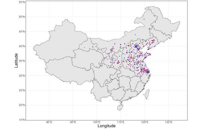
Figure 1: Map of China with geographic locations of pollution monitoring stations (in red) and meteorological stations (in blue).

The dataset we analyzed were derived from two different sources. The first source provided hourly $\text{PM}_{2.5}$ concentration measurements from $N=796$ pollution monitoring stations across northern and eastern China. As the response, we considered the log-transformed mean concentration across the period of July 1 - July 31 2021. The second source provided weather variables from $M=243$ meteorological stations at different locations from the pollution monitoring stations (hence the spatial misalignment). These included hourly temperature, precipitation, dewpoint, and wind information in the same period as the $\text{PM}_{2.5}$ concentration. For wind information, based on the original wind data consisting of hourly wind speed and dominant wind direction measured in degrees, we grouped them into four different directions and constructed corresponding variables to measure the average wind speed in each of the four directions; that is, north-west (NW), north-east (NE), south-east (SE), and south-west (SW). For instance, the NW covariate for the $i$-th meteorological station is computed as $\sum_{t=1}^{\mathcal{T}}WS_{it}1_{\{WD_{it}\in[270\degree,360\degree]\}}/\sum_{t=1}^{\mathcal{T}}1_{\{WD_{it}\in[270\degree,360\degree]\}}$ where $WS_{it}$ and $WD_{it}$ denote the wind speed and the dominant wind direction, respectively, of the $i$-th station at the $t$-th hour for $i=1,\cdots,243$, $t=1,\cdots,\mathcal{T}$ and $\mathcal{T}=24\text{ hours}\times 31\text{ days}=744\text{ hours}$. We then used the average hourly temperature, precipitation, and dewpoint together with these four wind variables as covariates in our model, resulting in $K=7$ meteorological covariates. Figure 1 presents the spatial misalignment between PM_2.5 observed at the pollution monitoring stations, and weather covariates observed at the meteorological stations.

Based on exploratory analysis (see Section LABEL:sec:appendix_supp_real_data of the supplementary material), we found that temperature, precipitation, and dewpoint are moderately correlated, while the remaining four wind variables also presented evidence of moderate cross-correlations between each other. This suggests it is important to account for spatial cross-correlations e.g., through the use of a generalized Kronecker product form in (2). There was also evidence of non-linear relationships between many of the meteorological covariates and PM_2.5; this was consistent with similar non-linear meteorological effects on air pollutant concentration that have been noted in other studies (Pearce et al.,, 2011; Yang et al.,, 2021). From these initial findings, we then applied CNR to the spatial linear mixed model (1) with $\nu_{\rho}=0.5$ and using natural cubic splines for all covariates, where the knots of the natural cubic splines were placed at the quintiles for each predicted meteorological covariate. We also examined a second order polynomial fit with $\bm{f}_{k}({x_{ik}})=(x_{ik},x_{ik}^{2})^{\top}$ for $k=1,\cdots,7$. The results of this fit are provided in the supplementary material, and are broadly consistent with those based on natural cubic splines discussed below.

Table 3 presents the estimated values of $\hat{\bm{\theta}}_{x,k}$ obtained in the first step of applying CNR for $k=1,\cdots,7$ (fixing $\nu_{k}=0.5$ based on exploratory analysis). Dewpoint had a much smaller estimated spatial range parameter than the other covariates, indicating that it had a relatively stronger spatial correlation, while temperature and dewpoint had larger estimated variances which reflected the larger scales of these two variables relative to the others. The estimated nugget parameters indicated that the four wind variables exhibited much more local variation than the other meteorological variables. The estimated between variable correlation matrix $\hat{\bm{R}}$ is given in Section LABEL:sec:appendix_supp_real_data of the supplementary material, and suggests that the generalized Kronecker product form was able to capture the positive correlations among the wind variables as well as the positive correlation between temperature and dewpoint.

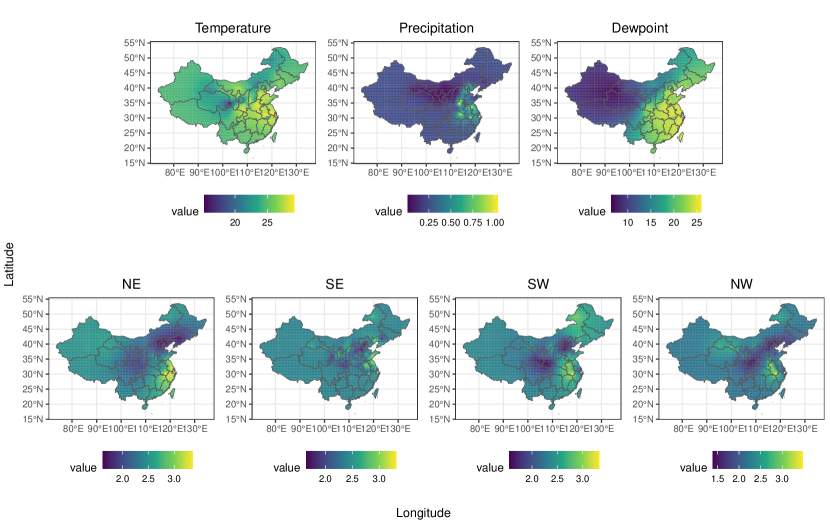
Figure 2: Spatial maps for the cokriging predictor of each meteorological covariate using CNR, based on the observed meteorological data $\bm{x}_{\tilde{S}}$ and the estimated parameters $\hat{\bm{\theta}}_{x}$.

Figure 2 presents spatial maps for the cokriging prediction of the meteorological covariates using the observed meteorological data $\bm{x}_{\tilde{S}}$. These were constructed by discretizing the map of China into a fine grid of pixels each of size $0.1\degree\times 0.1\degree$ , and then considering the centers of these pixels as the prediction locations. The noticeably higher variation in all of the maps towards the eastern part of China can be attributed to the concentration of the observed meteorological stations in that geographical region. Temperature was predicted to be fairly consistent across China, ranging from 15°C to 30°C in July 2021 during the summer. The map of precipitation showed that eastern China received more precipitation than the other parts; this is related to the flood that occurred in Henan Province in July 2021. In addition, the darker color in the northern part of the precipitation map indicated a much smaller predicted rainfall, which was expected given that this geographic area is part of the Gobi desert. The map of dewpoint demonstrated a clear decreasing trend from eastern China to western China. As for the wind variables, eastern China consisting of Shanghai City and Anhui, Jiangsu and Zhejiang provinces had stronger winds due to Typhoon In-fa in July 2021, which also contributed to the aforementioned flood.

For both the preliminary and secondary bootstrap in Section 3.1, we set $T=500$ and constructed 95% percentile confidence bands for the estimated conditional smoothers. We refer the readers to the supplementary material for details of the parametric bootstrap procedure when it involves knot placement for splines. For comparison, we used the 5-NMR method to estimate the conditional smoothers of the covariates, and constructed 95% confidence bands using the naive variance estimators of both CNR and 5-NMR.

Figure 3 presents the estimated conditional smoother for each covariate (based on setting the other covariates to their estimated mean values). Although both CNR and 5-NMR methods demonstrated non-linear relationships between the meteorological covariates and $\text{PM}_{2.5}$, their estimated trends were different for some of the meteorological covariates (which may be due to the biases of the 5-NMR estimates seen in the simulation studies of Section 4.1). The CNR conditional smoother showed that an increase in temperature in the range of 15°C to 20°C had a larger positive effect on $\text{PM}_{2.5}$ than the rise in temperature beyond 20°C. The positive effect is consistent with increases in temperature encouraging photochemical reactions that produce precursors to $\text{PM}_{2.5}$ (Jian et al.,, 2012). As for precipitation, CNR showed an obvious negative impact on $\text{PM}_{2.5}$ consistent with the idea of a washout effect (Guo et al.,, 2016). Dewpoint exhibited a U-shaped relationship with $\text{PM}_{2.5}$ based on both CNR and 5-NMR. Finally, the NE and SW covariates showed negative and positive effects, respectively, based on CNR, while their 5-NMR conditional smoothers suggested that they only have little effect on $\text{PM}_{2.5}$.

Turning to the 95% confidence bands, the proposed bootstrap confidence bands for CNR were wider than the corresponding bands based on the naive variance estimators of both CNR and 5-NMR for all meteorological covariates. This is consistent with the simulation results in Section 4.1, which suggested that the proposed bootstrap confidence bands better account for the uncertainty arising from spatial misalignment correction and the cross-correlation between the covariates. The confidence bands based on the naive variance estimator for CNR tended to be wider than the 5-NMR confidence bands near the lower and upper ends of the wind variables; such differences can be attributed to the lack of extreme values in the wind covariates’ predictions used for the fitting of the spatial linear mixed model in CNR.

In the supplementary material, we present additional results for 95% confidence bands based on the bias-corrected version of the naive variance estimator (Naive BC), the unadjusted bootstrap (Unadj-Bootstrap) and the non-cross-correlated bootstrap (NCC-Bootstrap) procedures. Our results again show that the Unadj-Bootstrap confidence bands were wider than the proposed bootstrap confidence bands, where the latter tended to be wider than the confidence bands based on the Naive BC and NCC-Bootstrap, noting both suffered from undercoverage issues in the simulation study in Section 4.1.

6 Conclusion

We have proposed a cokrig-and-regress method for estimating potentially non-linear relationships in a spatial linear mixed model, where the response and multiple correlated covariates are spatially misaligned. CNR replaces the unobserved covariates with their cokriging predictors before fitting the spatial regression model, where a generalized Kronecker product covariance matrix is employed to account for spatial cross-correlations between the multiple covariates. We also develop a parametric bootstrap approach to both perform bias correction on the CNR estimates of the spatial covariance parameters, and conduct statistical inference on the regression coefficients/smoothing functions. Simulation studies show that CNR performs strongly compared with the commonly used $L$-NMR method in estimating the regression coefficients, while the proposed parametric bootstrap confidence interval offers reasonable empirical coverage probability compared to intervals based on the naive variance estimator, the unadjusted bootstrap using biased spatial covariance parameter estimates, and a bootstrap that ignores the spatial cross-correlation between covariates. Application of CNR to spatially misaligned air pollution and meteorological data in China reveals complex, non-linear relationships between $\text{PM}_{2.5}$ concentration and several meteorological covariates.

A logical next step would be to extend CNR to handle non-Gaussian and/or areal responses and covariates e.g., through latent Gaussian models (Schliep and Hoeting,, 2013) or spatial autoregressive models (Tho et al.,, 2023). Also, given our proposed bootstrap approach for uncertainty quantification is relatively generic, then we can also handle other modifications for $\bm{f}_{k}(\cdot)$ such as penalized splines (Ruppert et al.,, 2003) and regression trees (Breiman et al.,, 1984), as well as different approaches to dealing with spatial correlations such as fixed rank kriging (see Ning et al.,, 2023, in the context of correcting for measurement error) and various flavors of Gaussian processes (Datta et al.,, 2016). The proposed CNR and bootstrap method could also be extended directly to handle spatial data that are partially misaligned, where $S\cap\tilde{S}\neq\emptyset$ and $S\neq\tilde{S}$, as well as misaligned spatio-temporal data (see for example Cismondi et al.,, 2013; Doan et al.,, 2015, for dealing with temporal misalignment of multiple time series). Finally, while this work has focused on the empirical performance of CNR, it would be interesting to theoretically study the asymptotic biases of the CNR estimates, perhaps leveraging from existing work on asymptotic bias analysis for the spatial linear mixed model with covariate measurement errors of Li et al., (2009), and subsequently develop results for the nominal coverage probability of bootstrap percentile intervals.

Declarations

Conflict of interest The authors declare no conflict of interest in this article.

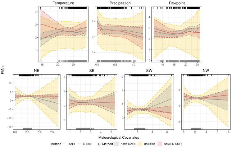
Figure 3: Estimated conditional smoothers for the seven meteorological covariates based on CNR (grey solid lines) and 5-NMR (red solid lines) included in the application to the China air pollution and meteorological data. Also shown are 95% confidence bands based on the naive variance estimator for CNR (shaded regions between dashed lines in grey), bootstrap percentile confidence bands for CNR (shaded regions between dashed lines in yellow) and the naive variance estimator for 5-NMR (shaded regions between dashed lines in red). The top rug represents the observed meteorological covariates $\tilde{\bm{x}}_{k}$, while the bottom rug represents the predicted meteorological covariates $\hat{\bm{x}}_{k}$ in CNR i.e., based on equation (6).

Table 1: Empirical Bias, empirical RMSE and the ratio ASE/ESD for CNR and 5-NMR estimators of $\beta_{k}$ in the simulation study. For CNR, the variance estimators include the naive variance estimator (Naive), the naive variance estimator but using bias-corrected estimates of the spatial covariance parameters (Naive BC), the proposed bootstrap procedure (Bootstrap), the unadjusted bootstrap procedure (Unadj-Bootstrap) and the non-cross-correlated bootstrap procedure (NCC-Bootstrap).

		Point estimation
	Method	$\beta_{1}=1$	$\beta_{2}=0.5$	$\beta_{3}=1$	$\beta_{4}=0.5$	$\beta_{5}=1$
Bias	CNR	$-0.0068$	$0.0021$	$-0.0070$	$0.0046$	$-0.0111$
	5-NMR	$-0.1529$	$-0.0752$	$-0.1591$	$-0.0665$	$-0.1580$
RMSE	CNR	$0.1733$	$0.1670$	$0.2068$	$0.2137$	$0.1948$
	5-NMR	$0.2516$	$0.2113$	$0.2705$	$0.2535$	$0.2872$
		ASE/ESD
Method	Variance estimator	$\beta_{1}=1$	$\beta_{2}=0.5$	$\beta_{3}=1$	$\beta_{4}=0.5$	$\beta_{5}=1$
CNR	Naive	0.7495	0.7749	0.7236	0.7811	0.7750
	Naive BC	0.5856	0.6060	0.5648	0.6091	0.6045
	Bootstrap	1.0896	1.0789	1.0300	1.0628	1.0928
	Unadj-Bootstrap	1.1984	1.1929	1.1244	1.1739	1.2047
	NCC-Bootstrap	1.0122	0.9868	0.8399	0.7687	0.8974
5-NMR	Naive	0.8096	0.8159	0.8571	0.8541	0.7827

Table 2: Empirical coverage probability and average interval widths for various 95% confidence intervals (CIs) of $\beta_{k}$ in the simulation study. For CNR, the CI methods include the Wald-type intervals using the naive variance estimator (Naive), the naive variance estimator but using bias-corrected estimates of the spatial covariance parameters (Naive BC), bootstrap percentile intervals (Bootstrap) and modified percentile intervals using the unadjusted bootstrap procedure (Unadj-Bootstrap) and the non-cross-correlated bootstrap procedure (NCC-Bootstrap).

	Method	CI method	$\beta_{1}=1$	$\beta_{2}=0.5$	$\beta_{3}=1$	$\beta_{4}=0.5$	$\beta_{5}=1$
Coverage	CNR	Naive	$0.8400$	$0.8650$	$0.8275$	$0.8875$	$0.8750$
		Naive BC	$0.7150$	$0.7375$	$0.7175$	$0.7625$	$0.7625$
		Bootstrap	$0.9525$	$0.9625$	$0.9600$	$0.9600$	$0.9550$
		Unadj-Bootstrap	$0.9725$	$0.9725$	$0.9675$	$0.9725$	$0.9825$
		NCC-Bootstrap	$0.9425$	$0.9475$	$0.8900$	$0.8850$	$0.9150$
	5-NMR	Naive	$0.7950$	$0.8500$	$0.8175$	$0.8750$	$0.8125$
Average Width	CNR	Naive	$0.5088$	$0.5073$	$0.5861$	$0.6543$	$0.5909$
		Naive BC	$0.3975$	$0.3967$	$0.4575$	$0.5102$	$0.4609$
		Bootstrap	$0.7326$	$0.6999$	$0.8264$	$0.8846$	$0.8290$
		Unadj-Bootstrap	$0.8057$	$0.7768$	$0.9042$	$0.9744$	$0.9136$
		NCC-Bootstrap	$0.6819$	$0.6395$	$0.6772$	$0.6411$	$0.6778$
	5-NMR	Naive	$0.6342$	$0.6316$	$0.7350$	$0.8189$	$0.7359$

Table 3: Estimated parameters $\hat{\bm{\theta}}_{x,k}$ of the marginal distribution for the seven meteorological covariates included in the application to the China air pollution and meteorological data.

Covariates	$\hat{\mu}_{k}$	$\hat{\sigma}^{2}_{k}$	$\hat{\alpha}_{k}$	$\hat{\tau}_{k}$
Temperature	$24.6902$	$7.3164$	$0.0028$	$0.0179$
Precipitation	$0.2460$	$0.0564$	$0.0049$	$0.0041$
Dewpoint	$16.5943$	$66.1287$	$0.0002$	$0.0651$
NE	$2.4590$	$0.2889$	$0.0013$	$0.5260$
SE	$2.3786$	$0.2060$	$0.0098$	$0.2742$
SW	$2.3631$	$0.2222$	$0.0026$	$0.2614$
NW	$2.1930$	$0.2638$	$0.0036$	$0.3933$

References

- Bakka et al., (2018) Bakka, H., Rue, H., Fuglstad, G.-A., Riebler, A., Bolin, D., Illian, J., Krainski, E., Simpson, D., and Lindgren, F. (2018). Spatial modeling with R-INLA: A review. Wiley Interdisciplinary Reviews: Computational Statistics, 10:e1443.
- Bonat and Jørgensen, (2016) Bonat, W. H. and Jørgensen, B. (2016). Multivariate covariance generalized linear models. Journal of the Royal Statistical Society. Series C (Applied Statistics), 65:649–675.
- Bonat et al., (2021) Bonat, W. H., Petterle, R. R., Balbinot, P., Mansur, A., and Graf, R. (2021). Modelling multiple outcomes in repeated measures studies: Comparing aesthetic eyelid surgery techniques. Statistical Modelling, 21:564–582.
- Breiman et al., (1984) Breiman, L., Friedman, J., Stone, C., and Olshen, R. (1984). Classification and regression trees. Taylor & Francis.
- Cao et al., (2023) Cao, J., He, S., and Zhang, B. (2023). Spatial linear regression with covariate measurement errors: Inference and scalable computation in a functional modeling approach. Journal of Computational and Graphical Statistics, pages 1–12.
- Cismondi et al., (2013) Cismondi, F., Fialho, A. S., Vieira, S. M., Reti, S. R., Sousa, J. M., and Finkelstein, S. N. (2013). Missing data in medical databases: Impute, delete or classify? Artificial Intelligence in Medicine, 58:63–72.
- Cressie and Wikle, (2015) Cressie, N. and Wikle, C. K. (2015). Statistics for spatio-temporal data. John Wiley & Sons.
- Datta et al., (2016) Datta, A., Banerjee, S., Finley, A. O., and Gelfand, A. E. (2016). Hierarchical nearest-neighbor Gaussian process models for large geostatistical datasets. Journal of the American Statistical Association, 111:800–812.
- Doan et al., (2015) Doan, T. K., Haslett, J., and Parnell, A. C. (2015). Joint inference of misaligned irregular time series with application to Greenland ice core data. Advances in Statistical Climatology, Meteorology and Oceanography, 1:15–27.
- Gneiting, (2013) Gneiting, T. (2013). Strictly and non-strictly positive definite functions on spheres. Bernoulli, 19:1327–1349.
- Greenstone et al., (2022) Greenstone, M., He, G., Jia, R., and Liu, T. (2022). Can technology solve the principal-agent problem? Evidence from China’s war on air pollution. American Economic Review: Insights, 4:54–70.
- Guo et al., (2016) Guo, L.-C., Zhang, Y., Lin, H., Zeng, W., Liu, T., Xiao, J., Rutherford, S., You, J., and Ma, W. (2016). The washout effects of rainfall on atmospheric particulate pollution in two Chinese cities. Environmental Pollution, 215:195–202.
- Jhun et al., (2015) Jhun, I., Coull, B. A., Schwartz, J., Hubbell, B., and Koutrakis, P. (2015). The impact of weather changes on air quality and health in the United States in 1994–2012. Environmental Research Letters, 10:084009.
- Jian et al., (2012) Jian, L., Zhao, Y., Zhu, Y.-P., Zhang, M.-B., and Bertolatti, D. (2012). An application of ARIMA model to predict submicron particle concentrations from meteorological factors at a busy roadside in Hangzhou, China. Science of The Total Environment, 426:336–345.
- Li et al., (2009) Li, Y., Tang, H., and Lin, X. (2009). Spatial linear mixed models with covariate measurement errors. Statistica Sinica, 19:1077–1093.
- Lindgren and Rue, (2015) Lindgren, F. and Rue, H. (2015). Bayesian spatial modelling with R-INLA. Journal of Statistical Software, 63:1–25.
- Liu et al., (2020) Liu, Y., Zhou, Y., and Lu, J. (2020). Exploring the relationship between air pollution and meteorological conditions in China under environmental governance. Scientific Reports, 10:14518.
- Madsen et al., (2008) Madsen, L., Ruppert, D., and Altman, N. S. (2008). Regression with spatially misaligned data. Environmetrics, 19:453–467.
- Martinez-Beneito, (2013) Martinez-Beneito, M. A. (2013). A general modelling framework for multivariate disease mapping. Biometrika, 100:539–553.
- Matérn, (1960) Matérn, B. (1960). Spatial variation : Stochastic models and their application to some problems in forest surveys and other sampling investigations. In Medd. Statens Skogsforskningsinstitut, volume 49.
- Ning et al., (2023) Ning, X., Hui, F. K. C., and Welsh, A. H. (2023). A double fixed rank kriging approach to spatial regression models with covariate measurement error. Environmetrics, 34:e2771.
- Pearce et al., (2011) Pearce, J., Beringer, J., Nicholls, N., Hyndman, R., and Tapper, N. (2011). Quantifying the influence of local meteorology on air quality using generalized additive models. Atmospheric Environment, 45:1328–1336.
- Pouliot, (2023) Pouliot, G. A. (2023). Spatial econometrics for misaligned data. Journal of Econometrics, 232:168–190.
- Reich et al., (2011) Reich, B. J., Eidsvik, J., Guindani, M., Nail, A. J., and Schmidt, A. M. (2011). A class of covariate-dependent spatiotemporal covariance functions for the analysis of daily ozone concentration. The Annals of Applied Statistics, 5:2425–2447.
- Rousset and Ferdy, (2014) Rousset, F. and Ferdy, J.-B. (2014). Testing environmental and genetic effects in the presence of spatial autocorrelation. Ecography, 37:781–790.
- Ruppert et al., (2003) Ruppert, D., Wand, M. P., and Carroll, R. J. (2003). Semiparametric regression. Cambridge Series in Statistical and Probabilistic Mathematics. Cambridge University Press.
- Salvana and Genton, (2020) Salvana, M. L. O. and Genton, M. G. (2020). Nonstationary cross-covariance functions for multivariate spatio-temporal random fields. Spatial Statistics, 37:100411.
- Schliep and Hoeting, (2013) Schliep, E. M. and Hoeting, J. A. (2013). Multilevel latent Gaussian process model for mixed discrete and continuous multivariate response data. Journal of Agricultural, Biological, and Environmental Statistics, 18:492–513.
- Stein and Corsten, (1991) Stein, A. and Corsten, L. C. A. (1991). Universal kriging and cokriging as a regression procedure. Biometrics, 47:575–587.
- Szpiro et al., (2011) Szpiro, A. A., Sheppard, L., and Lumley, T. (2011). Efficient measurement error correction with spatially misaligned data. Biostatistics, 12:610–623.
- Tho et al., (2023) Tho, Z. Y., Ding, D., Hui, F. K. C., Welsh, A. H., and Zou, T. (2023). On the robust estimation of spatial autoregressive models. Econometrics and Statistics.
- Yang et al., (2021) Yang, Z., Yang, J., Li, M., Chen, J., and Ou, C.-Q. (2021). Nonlinear and lagged meteorological effects on daily levels of ambient PM2.5 and O3: Evidence from 284 Chinese cities. Journal of Cleaner Production, 278:123931.