Diagonal of Pseudoinverse of Graph Laplacian: Fast Estimation and Exact Results

Abstract

The diagonal entries of pseudoinverse of the Laplacian matrix of a graph appear in many important practical applications, since they contain much information of the graph and many relevant quantities can be expressed in terms of them, such as Kirchhoff index and current flow centrality. However, a naïve approach for computing the diagonal of a matrix inverse has cubic computational complexity in terms of the matrix dimension, which is not acceptable for large graphs with millions of nodes. Thus, rigorous solutions to the diagonal of the Laplacian matrices for general graphs, even for particluar graphs are much less. In this paper, we propose a theoretically guaranteed estimation algorithm, which approximates all diagonal entries of the pseudoinverse of a graph Laplacian in nearly linear time with respect to the number of edges in the graph. We execute extensive experiments on real-life networks, which indicate that our algorithm is both efficient and accurate. Also, we determine exact expressions for the diagonal elements of pseudoinverse of the Laplacian matrices for Koch networks and uniform recursive trees, and compare them with those obtained by our approximation algorithm. Finally, we use our algorithm to evaluate the Kirchhoff index of three deterministic model networks, for which the Kirchhoff index can be rigorously determined. These results further show the effectiveness and efficiency of our algorithm.

1 Introduction

As a typical representation of a graph, the Laplacian matrix $\bm{\mathit{L}}$ encapsulates much useful structural and dynamical information of the graph [1]. In addition to $\bm{\mathit{L}}$ itself, its pseudoinverse $\bm{\mathit{L}}^{\dagger}$ is also a powerful tool in network science [2], which arises in various aspects, such as random walks [3] and electrical networks [4]. Particularly, the diagonal entries of $\bm{\mathit{L}}^{\dagger}$ appear frequently in diverse applications, for example, node centrality from both structural [5, 6, 7, 8] and dynamical [9, 10] perspectives. Moreover, a lot of other interesting quantities of a graph are also encoded in the diagonal entries of $\bm{\mathit{L}}^{\dagger}$. For example, the sum of diagonal entries of $\bm{\mathit{L}}^{\dagger}$ (trace of $\bm{\mathit{L}}^{\dagger}$) is in fact the Kirchhoff index [11], an invariant of a graph, which has found wide applications. First, it can serve as measures of the overall connectedness of a network [12], the edge importance of complex networks [13], and the robustness of first-order noisy networks [14] that has attracted much attension from the cybernetics community [15, 16, 17]. Besides, the popular current flow centrality [18, 19] or information centrality [20] can also be represented in terms of the diagonal entries of $\bm{\mathit{L}}^{\dagger}$.

In order to achieve better effects of the applications for the diagonal entries of $\bm{\mathit{L}}^{\dagger}$ for a graph with $N$ nodes, the first step is to compute or evaluate the diagonal of $\bm{\mathit{L}}^{\dagger}$. A straightforward computation of $\bm{\mathit{L}}^{\dagger}$ involves inverting a perturbed Laplacian matrix $\bm{\mathit{L}}+\bm{\mathit{J}}$, where $\bm{\mathit{J}}$ is the $N\times N$ matrix with every entry being $1$ [21], which costs $O(N^{3})$ operations and $O(N^{2})$ memories and thus is prohibitive for relatively large graphs with millions of nodes. In [22], an incremental approach was proposed to compute $\bm{\mathit{L}}^{\dagger}$. Although for general cases, this method performs better than the standard approach, for the worst case its computation cost is still $O(N^{3})$. To reduce the computational complexity, some approximation algorithms were designed to estimate $\bm{\mathit{L}}^{\dagger}$ [23] or diagonal of a more general matrix [24, 25, 26], which have low complexity but no approximation guarantee. Thus, a theoretically guaranteed estimation algorithm for approximating $\bm{\mathit{L}}^{\dagger}$ is imperative.

As shown above, many interesting quantities, such as Kirchhoff index, are closely related to the diagonal elements of matrix $\bm{\mathit{L}}^{\dagger}$ of a graph $\mathcal{G}$, the behaviors of which characterize various dynamical processes defined on $\mathcal{G}$, including random walks, first-order noisy consensus [14, 27, 28], and so on [29]. However, the heavy demand on time and computer memory for inverting a matrix make it almost impossible to obtain exact results for the diagonal of $\bm{\mathit{L}}^{\dagger}$ for a general large graph. It is thus of significant importance to seek for some particular graphs with some remarkable properties observed for real-world networks, the diagonal elements of $\bm{\mathit{L}}^{\dagger}$ for which can be determined exactly by using computationally cheaper approaches. In addition to uncover the dependence of these primary quantities (e.g., Kirchhoff index) on the system size, rigorous results are also very useful as benchmark results for testing heuristic algorithms for computing the diagonal elements of a matrix inversion. Unfortunately, to the best of our knowledge, exact results for the diagonal of matrix $\bm{\mathit{L}}^{\dagger}$ for scale-free small-world graphs is lacking, in spite of the fact that scale-free and small-world properties are ubiquitous in real networked systems [29].

In this paper, we focus on approximation method for computing the diagonal of the pseudoinverse $\bm{\mathit{L}}^{\dagger}$ of a general graph, as well as exact results for diagonal of $\bm{\mathit{L}}^{\dagger}$ for two special graphs. Our main contributions are as follows.

• We introduce an approximation algorithm to compute the diagonal of the pseudoinverse $\bm{\mathit{L}}^{\dagger}$ of the Laplacian matrix $\bm{\mathit{L}}$ of a graph with $N$ nodes and $M$ edges. It returns an approximation of the actual diagonal entries of $\bm{\mathit{L}}^{\dagger}$ in nearly linear time with respect to $M$. Moreover, we prove that our approach has a guarantee for error bounds with a high probability.

• We perform extensive experiments on real-world networks, the results of which show that compared to the direct approach for inverting matrix, the proposed approximation method is both effective and efficient.

• We derive exact expressions for the diagonal elements of $\bm{\mathit{L}}^{\dagger}$ for two deterministic networks, the scale-free small-world Koch networks [30] and the uniform recursive trees [31], and compare them with the results obtained by our approximation algorithm.

• We apply our algorithm to estimate the Kirchhoff index of three networks, Koch networks, uniform recursive trees, and pseudofractal scale-free web [32, 33], the Kirchhoff index of which can be explicitly determined. These further demonstrate the efficiency and accuracy of our algorithm.

2 Preliminaries

In this section, we briefly introduce some basic concepts about graphs, including spanning rooted forest, electrical network, resistance distance, Laplacian matrix and its pseudoinverse, spectral properties of Laplacian and its pseudoinverse, interpretations of pseudoinverse for graph Lapcacian.

2.1 Graphs and Spanning Rooted Forests

Let $\mathcal{G}=(V,E,w)$ denote a connected undirected weighted graph or network, where $V$ is the set of nodes (vertices) $E$ is the set of edges (links), and $w:E\to\mathbb{R}_{+}$ is the positive edge weight function, with $w_{e}$ being the weight for edge $e$. Then, there are total $N=|V|$ vertices and $M=|E|$ edges in graph $\mathcal{G}$. We use $u\sim v$ to indicate that two vertices $u$ and $v$ are connected by an edge. Let $w_{\max}$ and $w_{\min}$ denote the maximum edge weight and minimum edge weight, respectively. Namely, $w_{\max}=\max_{e\in E}w_{e}$ and $w_{\min}=\min_{e\in E}w_{e}$.

For a graph $\mathcal{G}=(V,E,w)$, a subgraph $\mathcal{H}$ of $\mathcal{G}$ is a graph, the node and edge sets of which are subsets of $V$ and $E$, respectively. The product of the weights of the edges in $\mathcal{H}$ is called the weight of $\mathcal{H}$, denoted by $\varepsilon(\mathcal{H})$. The weight of a subgraph $\mathcal{H}$ with no edges is set to be 1. For any nonempty set $S$ of subgraphs, its weight is defined as $\varepsilon(S)=\sum_{\mathcal{H}\in S}\varepsilon(\mathcal{H})$. The weight of the empty set is set to be zero [34]. A spanning subgraph $\mathcal{G}^{\prime}$ of $\mathcal{G}$ is a subgraph of $\mathcal{G}$ with the same node set $V$ and an edge set $E^{\prime}\subseteq E$. A spanning tree of $\mathcal{G}$ is a spanning subgraph of $\mathcal{G}$ that is a tree. A spanning forest on $\mathcal{G}$ is a spanning subgraph of $\mathcal{G}$ that is a disjoint union of trees. Here an isolated vertex is considered as a tree. A spanning rooted forest of $\mathcal{G}$ is a spanning forest of $\mathcal{G}$ with a particular node (a root) marked in each tree. Let $\mathcal{F}_{x}$, $x\geq 1$, be the set of spanning rooted forests of $\mathcal{G}=(V,E,w)$, with each spanning rooted forest having exactly $x$ trees. Let $\mathcal{F}_{x}^{ij}$ be the set of spanning rooted forests of $\mathcal{G}=(V,E,w)$ with $x$ trees, one of which is rooted at $i$ and contains $j$. And let $\mathcal{F}_{x}^{ii}$ be the set of spanning rooted forests of $\mathcal{G}=(V,E,w)$ containing $x$ trees, with one tree including $i$ and being rooted at $i$.

2.2 Electrical Networks and Resistance Distances

For an arbitrary undirected weighted graph $\mathcal{G}=(V,E,w)$, we can define an electrical network $\bar{\mathcal{G}}=(V,E,r)$, which is obtained from $\mathcal{G}$ by looking upon edges as resistors and considering vertices as junctions between resistors [35], with the resistor of an associated edge $e$ being $r_{e}=w_{e}^{-1}$. For graph $\mathcal{G}$, the resistance distance $r_{ij}$ between two vertices $i$ and $j$ is defined as the effective resistance between $i$ and $j$ in the corresponding electrical network $\bar{\mathcal{G}}$ [11], which is equal to the potential difference between $i$ and $j$ when a unit current enters one vertex and leaves the other one. The resistance distances of a graph have many interesting properties. For example, they obey the following Foster’s theorem [36].

Lemma 2.1.

Let $\mathcal{G}=(V,E,w)$ be a simple connected graph with $N$ nodes. Then the sum of weight times resistance distance over all pairs of adjacent vertices in $\mathcal{G}$ satisfies

$$\sum_{i\sim j}w_{ij}\times r_{ij}=N-1.$$

Two key quantities related to resistance distances are the resistance distance of a given node and Kirchhoff index.

Definition 2.2.

For an undirected weighted graph $\mathcal{G}=(V,E,w)$, the resistance distance $r_{i}$ of a node $i$ is the sum of resistance distances between $i$ and all other nodes:

$$r_{i}:=\sum^{N}_{j=1}r_{ij}\,.$$

The Kirchhoff index $\delta$ of $\mathcal{G}$ is the sum of resistance distances over all the $N(N-1)/2$ pairs of nodes:

$$\delta:=\sum_{i=1}^{N}\sum_{j=i}^{N}r_{ij}\,.$$

Both quantities appear in practical applications. The reciprocal of $r_{i}$ times $N$ is in fact the current flow centrality [37, 19] of node $i$, which is equivalent to information centrality [38, 39] of $i$. While the Kirchhoff index can be applied to measure the overall connectedness of a network [12], the robustness of first-order noisy networks [14], as well as the edge importance of complex networks [13].

2.3 Graph Laplacian Matrix

Mathematically, the topological and weighted properties of a graph $\mathcal{G}$ are encoded in its generalized adjacency matrix $\bm{\mathit{A}}$ with the entry $a_{ij}$ denoting the adjacency relation between vertices $i$ and $j$. If vertices $i$ and $j$ are linked to each other by an edge $e$, then $a_{ij}=a_{ji}=w_{e}>0$. Otherwise, $a_{ij}=a_{ji}=0$ indicates that vertices $i$ and $j$ are not adjacent. In a weighted graph $\mathcal{G}$, the strength $s_{i}$ of a vertex $i$ is defined by $s_{i}=\sum_{j=1}^{N}a_{ij}$ [40]. The diagonal strength matrix of graph $\mathcal{G}$ is defined to be ${\SS}={\rm diag}(s_{1},s_{2},\ldots,s_{N})$, and the Laplacian matrix of $\mathcal{G}$ is ${\bm{\mathit{L}}}={\SS}-{\bm{\mathit{A}}}$.

Let $\bm{\mathit{B}}\in\mathbb{R}^{|E|\times|V|}$ be the incidence matrix of $\mathcal{G}$. For each edge $e$ with two end vertices $i$ and $j$, a direction is assigned arbitrarily. Let $\bm{\mathit{b}}_{e}^{\top}$ be the row of matrix $\bm{\mathit{B}}$ associated with edge $e$. Then the element $b_{eu}$ at row corresponding to edge $e$ and column corresponding to vertex $u$ is defined as follows: $b_{eu}=1$ if vertex $u$ is the tail of edge $e$, $b_{eu}=-1$ if vertex $u$ is the head of edge $e$, and $b_{eu}=0$ otherwise. Let $\bm{\mathit{e}}_{u}$ be the $u$-th canonical basis of the space $\mathbb{R}^{|V|}$, then for an edge $e$ connecting two vertices $i$ and $j$, $\bm{\mathit{b}}_{e}$ can also be recast as $\bm{\mathit{b}}_{e}=\bm{\mathit{e}}_{i}-\bm{\mathit{e}}_{j}$. Let $\bm{\mathit{W}}\in\mathbb{R}^{|E|\times|E|}$ be a diagonal matrix with the diagonal entry $(e,e)$ being $w_{e}$. Then the Laplacian matrix $\bm{\mathit{L}}$ of graph $\mathcal{G}$ can be written as $\bm{\mathit{L}}=\bm{\mathit{B}}^{T}\bm{\mathit{W}}\bm{\mathit{B}}=\sum_{e\in E}w_{e}\bm{\mathit{b}}_{e}\bm{\mathit{b}}_{e}^{\top}$. Let $\mathbf{1}$ denote the vector of appropriate dimensions with all entries being ones, and let $\bm{\mathit{J}}$ be the matrix defined by $\bm{\mathit{J}}=\mathbf{1}\mathbf{1}^{\top}$. Moreover, let $\mathbf{0}$ and $\mathbf{O}$ denote, respectively, the zero vector and zero matrix. Since ${\SS}\mathbf{1}={\bm{\mathit{A}}}\mathbf{1}$, then ${\bm{\mathit{L}}}\mathbf{1}=\mathbf{0}$ and ${\bm{\mathit{L}}}\bm{\mathit{J}}=\bm{\mathit{J}}{\bm{\mathit{L}}}=\mathbf{O}$.

2.4 Spectrum of Graph Laplacian and its Pseudoinverse

For a connected undirected graph $\mathcal{G}=(V,E,w)$, its Laplacian matrix $\bm{\mathit{L}}$ is symmetric and positive semidefinite. All its eigenvalues are non-negative, with a unique zero eigenvalue. Let $0=\lambda_{1}<\lambda_{2}\leq\lambda_{3}\leq\dots\leq\lambda_{N-1}\leq\lambda_{N}$ be the $N$ eigenvalues of $\bm{\mathit{L}}$, and let $\bm{\mathit{u}}_{k}$, $k={1,2,\dots,N}$, be their corresponding mutually orthogonal unit eigenvectors. Then, $\bm{\mathit{L}}$ admits the following spectral decomposition: $\bm{\mathit{L}}=\sum_{k=1}^{N}\lambda_{k}\bm{\mathit{u}}_{k}\bm{\mathit{u}}_{k}^{\top}$, which means that the $ij$ entry $\bm{\mathit{L}}_{ij}$ of $\bm{\mathit{L}}$ is $\bm{\mathit{L}}_{ij}=\sum_{k=2}^{N}\lambda_{k}\bm{\mathit{u}}_{ki}\bm{\mathit{u}}_{kj}$, where $\bm{\mathit{u}}_{ki}$ is the $i$th component of vector $\bm{\mathit{u}}_{k}$. It can be verified [41] that among all $N$-node connected undirected weighted graphs $\mathcal{G}=(V,E,w)$, the largest eigenvalue $\lambda_{N}$ of Laplacian matrix satisfies $\lambda_{N}\leq Nw_{\max}$, with equality if and only if $\mathcal{G}$ is the $N$-node complete graph, where the weight of every edge is $w_{\max}$.

Having $0$ as an eigenvalue, $\bm{\mathit{L}}$ is singular and cannot be inverted. As a substitute for the inverse we use the Moore-Penrose generalized inverse of $\bm{\mathit{L}}$, that we simply call pseudoinverse of $\bm{\mathit{L}}$ [42]. As customary, we use $\bm{\mathit{L}}^{\dagger}$ to denote its pseudoinverse, which can be written as

$$\bm{\mathit{L}}^{\dagger}=\sum_{k=2}^{N}\frac{1}{\lambda_{k}}\bm{\mathit{u}}_{k}\bm{\mathit{u}}_{k}^{\top}.$$ (1)

Then, the entry $\bm{\mathit{L}}^{\dagger}_{ij}$ of $\bm{\mathit{L}}^{\dagger}$ at row $i$ and column $j$ can be expressed as $\bm{\mathit{L}}^{\dagger}_{ij}=\sum_{k=2}^{N}\frac{1}{\lambda_{k}}\bm{\mathit{u}}_{ki}\bm{\mathit{u}}_{kj}$. Thus, the $i$th diagonal entry $\bm{\mathit{L}}^{\dagger}_{ii}$ of $\bm{\mathit{L}}^{\dagger}$ is equal to $\sum_{k=2}^{N}\frac{1}{\lambda_{k}}\bm{\mathit{u}}^{2}_{ki}$. Since $\bm{\mathit{L}}$ is symmetric, it is the same with $\bm{\mathit{L}}^{\dagger}$ [43], which can also be seen from the fact $\bm{\mathit{L}}^{\dagger}_{ij}=\bm{\mathit{L}}^{\dagger}_{ji}=\sum_{k=2}^{N}\frac{1}{\lambda_{k}}\bm{\mathit{u}}_{ki}\bm{\mathit{u}}_{kj}$.

Note that for a general symmetric matrix, it shares the same null space as its Moore-Penrose generalized inverse [42]. Since ${\bm{\mathit{L}}}\mathbf{1}=\mathbf{0}$, it turns out that ${\bm{\mathit{L}}}^{\dagger}\mathbf{1}=\mathbf{0}$. Considering $\bm{\mathit{J}}=\mathbf{1}\mathbf{1}^{\top}$, we further obtain ${\bm{\mathit{L}}}\bm{\mathit{J}}=\bm{\mathit{J}}{\bm{\mathit{L}}}={\bm{\mathit{L}}}^{\dagger}\bm{\mathit{J}}=\bm{\mathit{J}}{\bm{\mathit{L}}}^{\dagger}=\mathbf{O}$. Let $\bm{\mathit{I}}$ be the identity matrix of approximate dimensions. Using the spectral decompositions of $\bm{\mathit{L}}$ and ${\bm{\mathit{L}}}^{\dagger}$, it is not difficult to verify that

$$\left(\bm{\mathit{L}}+\frac{1}{N}\bm{\mathit{J}}\right)\left(\bm{\mathit{L}}^{\dagger}+\frac{1}{N}\bm{\mathit{J}}\right)=\bm{\mathit{I}}.$$

Then, it follows that

$$\bm{\mathit{L}}^{\dagger}=\left(\bm{\mathit{L}}+\frac{1}{N}\bm{\mathit{J}}\right)^{-1}-\frac{1}{N}\bm{\mathit{J}},$$ (2)

which was explicitly stated in [21] and was implicitly applied in [44, 37]. Another useful consequence of the above two equalities is

$$\bm{\mathit{L}}\bm{\mathit{L}}^{\dagger}=\bm{\mathit{L}}^{\dagger}\bm{\mathit{L}}=\bm{\mathit{I}}-\frac{1}{N}\bm{\mathit{J}}\,,$$ (3)

which will be used in the following text.

2.5 Interpretations of Entries of Pseudoinverse for Graph Laplacian

For a graph, many key quantities are encoded in the entries of the pseudoinverse for its Laplacian matrix, which in turns provide interpretations for the pseudoinverse $\bm{\mathit{L}}^{\dagger}$ for graph Laplacian $\bm{\mathit{L}}$ from different angles.

2.5.1 Topological interpretation

Chebotarev and Shamis [34] offer a topological explanation for $\bm{\mathit{L}}^{\dagger}$ by representing the entries $\bm{\mathit{L}}^{\dagger}_{ij}$ and $\bm{\mathit{L}}^{\dagger}_{ii}$ of $\bm{\mathit{L}}^{\dagger}$ in terms of the weight of spanning rooted forests:

$$\bm{\mathit{L}}^{\dagger}_{ij}=\frac{\varepsilon(\mathcal{F}_{2}^{ij})-\frac{1}{N}\varepsilon(\mathcal{F}_{2})}{\varepsilon(\mathcal{F}_{1})}$$ (4)

and

$$\bm{\mathit{L}}^{\dagger}_{ii}=\frac{\varepsilon(\mathcal{F}_{2}^{ii})-\frac{1}{N}\varepsilon(\mathcal{F}_{2})}{\varepsilon(\mathcal{F}_{1})}.$$ (5)

In [6, 7] Ranjan and Zhang put forth a measure for node centrality, called topological centrality. For a node $i$, its topological centrality is defined as $1/\bm{\mathit{L}}^{\dagger}_{ii}$. Moreover, many other authors also use $\bm{\mathit{L}}^{\dagger}_{ii}$ to measure node importance in different scenarios [5, 8].

2.5.2 Explanations from viewpoint of electrical networks

Various quantities related to electrical networks are relevant to the pseudoinverse $\bm{\mathit{L}}^{\dagger}$ for graph Laplacian $\bm{\mathit{L}}$. In the context of effective resistances, resistance distance $r_{ij}$ between any pair of nodes $i$ and $j$, the resistance distance $r_{i}$ of a node $i$, and the Kirchhoff index of the whole graph are all encoded in the entries of $\bm{\mathit{L}}^{\dagger}$. First, the resistance distance $r_{ij}$ between two vertices $i$ and $j$ can be written in terms of the entries of $\bm{\mathit{L}}^{\dagger}$ as $r_{ij}=\bm{\mathit{L}}^{\dagger}_{ii}+\bm{\mathit{L}}^{\dagger}_{jj}-\bm{\mathit{L}}^{\dagger}_{ij}-\bm{\mathit{L}}^{\dagger}_{ji}$ [11]. Second, the Kirchhoff index $\delta$ of a graph $\mathcal{G}$ with $N$ nodes is equal to $N$ times the trace of $\mathrm{Tr}\left(\bm{\mathit{L}}^{\dagger}\right)$ of matrix $\bm{\mathit{L}}^{\dagger}$ [11], that is,

$$\delta=N\,\mathrm{Tr}\left(\bm{\mathit{L}}^{\dagger}\right)=N\sum_{i=1}^{N}\bm{\mathit{L}}^{\dagger}_{ii}\,.$$ (6)

Finally, the resistance distance $r_{i}$ of node $i$ can also be expressed in terms of the diagonal elements of $\mathrm{Tr}\left(\bm{\mathit{L}}^{\dagger}\right)$ [45]:

$$R_{i}=N\,\bm{\mathit{L}}^{\dagger}_{ii}+\mathrm{Tr}\left(\bm{\mathit{L}}^{\dagger}\right)=N\left(\bm{\mathit{L}}^{\dagger}_{ii}+\sum_{j=1}^{N}\bm{\mathit{L}}^{\dagger}_{jj}\right),$$ (7)

which implies

$$\bm{\mathit{L}}^{\dagger}_{ii}=\frac{R_{i}-\mathrm{Tr}\left(\bm{\mathit{L}}^{\dagger}\right)}{N}.$$ (8)

Thus, $\bm{\mathit{L}}^{\dagger}_{ii}$ indicates how close node $i$ is within the graph. The above formula implies that the ordering of nodes by structural centrality is identical to the ordering of nodes by current flow centrality and information centrality.

In addition to the aforementioned interpretations for $\bm{\mathit{L}}^{\dagger}$, there are many other representations or explanations for the entries of $\bm{\mathit{L}}^{\dagger}$. For example, it was shown that the pseudoinverse $\bm{\mathit{L}}^{\dagger}$ for graph Laplacian also has persuasive interpretations in potential of nodes in an electrical network [23, 45], expected number of visit times of random walks [6, 7], and many others [46].

3 Related work

As shown above, the pseudoinverse $\bm{\mathit{L}}^{\dagger}$ for graph Laplacian $\bm{\mathit{L}}$ arises in various application settings, and many relevant quantities can be expressed in terms of the entries of $\bm{\mathit{L}}^{\dagger}$. Particularly, the diagonal of $\bm{\mathit{L}}^{\dagger}$ contains much structural and dynamical information about a graph. For example, the diagonal of $\bm{\mathit{L}}^{\dagger}$ is sufficient to compute the structural centrality, current flow centrality, information centrality, and Kirchhoff index of a graph. It it thus of great interest to compute matrix $\bm{\mathit{L}}^{\dagger}$. However, computing $\bm{\mathit{L}}^{\dagger}$ is a theoretical challenge. By virtue of (1) and (2), naïve methods for computing $\bm{\mathit{L}}^{\dagger}$ of a graph involve either calculating the eigenvalues and eigenvector of $\bm{\mathit{L}}$ or inverting a suitable perturbed version $\bm{\mathit{L}}+\frac{1}{n}\bm{\mathit{J}}$ of $\bm{\mathit{L}}$ and then subtracting the perturbation $\frac{1}{n}\bm{\mathit{J}}$. Both straightforward ways to compute $\bm{\mathit{L}}^{\dagger}$ cost $O(N^{3})$ time, which are infeasible for large-scale networks with millions of nodes and edges.

In order to speed up the computation of matrix $\bm{\mathit{L}}^{\dagger}$, a lot of endeavors have been devoted to fast algorithms for evaluating $\bm{\mathit{L}}^{\dagger}$. In [22], an incremental approach was designed to compute $\bm{\mathit{L}}^{\dagger}$. For general cases, this method performs better than the common approaches, but for the worst case it still has a computation cost of $O(N^{3})$. Moreover, several approximation algorithms were presented to estimate matrix $\bm{\mathit{L}}^{\dagger}$ [23] or the diagonal entries of a more general matrix [24, 25, 26], with an aim to reduce the computational complexity. Although these algorithms have low complexity, they have no approximation guarantee. Finally, many algorithms were developed to address a related issue of estimating the trace of a matrix [47, 48, 49]. However, these algorithms do not apply to evaluate the diagonal of $\bm{\mathit{L}}^{\dagger}$. It is thus desirable to propose an effective and efficient algorithm for approximating $\bm{\mathit{L}}^{\dagger}$ that provides error bounds on the diagonal entries. This is the main research subject of the present paper.

In order to obtain an exact expression for every diagonal element $\bm{\mathit{L}}_{ii}^{\dagger}$, $i={1,2,\dots,N}$, of the pseudoinverse of $\bm{\mathit{L}}$ for a graph with $N$ vertices, one may determine all $N-1$ non-zero eigenvalues of $\bm{\mathit{L}}$ and their corresponding mutually orthogonal unit eigenvectors. Making use of the approach similar to that in [50], it is not difficult to derive a rigorous formular for each $\bm{\mathit{L}}_{ii}^{\dagger}$ for some particular graphs, including the path graph, the ring graph, the star graph, and the complete graph, since the eigenvalues and eigenvectors of their Laplacian matrices can be obtained explicitly. However, these graphs cannot mimic real networks, most of which display the striking scale-free small-world behaviors [29]. Thus far, rigorous solution for $\bm{\mathit{L}}_{ii}^{\dagger}$ associated with scale-free small-world networks is still missing. One the other hand, some real networks (e.g., power grid) are exponential with their degree distribution decaying exponentially [51], but related analytical work for $\bm{\mathit{L}}_{ii}^{\dagger}$ is also much less.

4 Fast Algorithm for Approximating the Diagonal of Pseudoinverse of Graph Laplacian

In this section, we propose an algorithm to compute an approximation of all diagonal entries of $\bm{\mathit{L}}^{\dagger}$ in nearly linear time with respect to the number of edges. Our algorithm has an error guarantee with a high probability.

To achieve our goal, we first reduce the problem for computing a diagonal entry of $\bm{\mathit{L}}^{\dagger}$ to calculating the $\ell_{2}$ norm of a vector. Then using the techniques of random projections and linear system solvers, we estimate the $\ell_{2}$ norm, aiming to reduce the computation complexity. We now express $\bm{\mathit{L}}^{\dagger}_{uu}$ in an Euclidian norm. According to (3) and the relation $\bm{\mathit{L}}\bm{\mathit{J}}=\mathbf{O}$, we obtain

$$\bm{\mathit{L}}^{\dagger}_{uu}=\bm{\mathit{e}}_{u}^{T}\bm{\mathit{L}}^{\dagger}\bm{\mathit{L}}\bm{\mathit{L}}^{\dagger}\bm{\mathit{e}}_{u}=\bm{\mathit{e}}_{u}^{T}\bm{\mathit{L}}^{\dagger}\bm{\mathit{B}}^{T}\bm{\mathit{W}}\bm{\mathit{B}}\bm{\mathit{L}}^{\dagger}\bm{\mathit{e}}_{u}$$

$$= \bm{\mathit{e}}_{u}^{T}\bm{\mathit{L}}^{\dagger}\bm{\mathit{B}}^{T}\bm{\mathit{W}}^{1/2}\bm{\mathit{W}}^{1/2}\bm{\mathit{B}}\bm{\mathit{L}}^{\dagger}\bm{\mathit{e}}_{u}=\|\bm{\mathit{W}}^{1/2}\bm{\mathit{B}}\bm{\mathit{L}}^{\dagger}\bm{\mathit{e}}_{u}\|^{2}.$$

In this way, we have reduced the computation of a diagonal element $\bm{\mathit{L}}^{\dagger}_{uu}$ of $\bm{\mathit{L}}^{\dagger}$ to evaluating the $\ell_{2}$ norm of a vector in $\mathbb{R}^{M}$. However, through using this $\ell_{2}$ norm, the complexity for exactly computing all diagonal elements is still very high. Fortunately, applying the Johnson-Lindenstrauss lemma [52, 53, 54], the $\ell_{2}$ norm can be nearly preserved by projecting the vector onto a low-dimensional subspace, while the computational cost is significantly reduced. For consistency, we introduce the Johnson-Lindenstrauss lemma [52, 53, 54].

Lemma 4.1.

Given fixed vectors $\bm{\mathit{v}}_{1},\bm{\mathit{v}}_{2},\ldots,\bm{\mathit{v}}_{N}\in\mathbb{R}^{M}$ and $\epsilon>0$, let $\bm{\mathit{Q}}_{k\times M}$ be a random $\pm 1/\sqrt{k}$ matrix (i.e., independent Bernoulli entries) with $k\geq 24\log N/\epsilon^{2}$. Then with probability at least $1-1/N$,

$$(1-\epsilon)\|\bm{\mathit{v}}_{i}-\bm{\mathit{v}}_{j}\|_{2}^{2}\leq\|\bm{\mathit{Q}}\bm{\mathit{v}}_{i}-\bm{\mathit{Q}}\bm{\mathit{v}}_{j}\|_{2}^{2}\leq(1+\epsilon)\|\bm{\mathit{v}}_{i}-\bm{\mathit{v}}_{j}\|_{2}^{2}$$

for all pairs $i,j\leq N$.

Let $\bm{\mathit{Q}}$ be a $k\times M$ random projection matrix. By Lemma 4.1, $\|\bm{\mathit{Q}}\bm{\mathit{W}}^{\frac{1}{2}}\bm{\mathit{B}}\bm{\mathit{L}}^{\dagger}\bm{\mathit{e}}_{u}\|$ is a good approximation for $\|\bm{\mathit{W}}^{\frac{1}{2}}\bm{\mathit{B}}\bm{\mathit{L}}^{\dagger}\bm{\mathit{e}}_{u}\|$. Here we can use sparse matrix multiplication to compute $\bm{\mathit{Q}}\bm{\mathit{W}}^{\frac{1}{2}}\bm{\mathit{B}}$, which takes $2M\times 24\log N/\epsilon^{2}+M$ time, since $\bm{\mathit{B}}$ has $2M$ non-zero elements and $\bm{\mathit{W}}^{\frac{1}{2}}$ is a diagonal matrix. However, computing $\bm{\mathit{Z}}=\bm{\mathit{Q}}\bm{\mathit{W}}^{\frac{1}{2}}\bm{\mathit{B}}\bm{\mathit{L}}^{\dagger}$ directly involves calculating $\bm{\mathit{L}}^{\dagger}$. In order to avoid calculating $\bm{\mathit{L}}^{\dagger}$, we resort to the nearly-linear time solver [55, 56] as stated in the following lemma. In the sequel, we use the notation $\widetilde{O}(\cdot)$ to hide $\mathrm{poly}(\log N)$ factors.

Lemma 4.2.

There is an algorithm $\bm{\mathit{x}}=\mathtt{LaplSolve}(L,\bm{\mathit{y}},\theta)$ which takes a Laplacian matrix $\bm{\mathit{L}}$, a column vector $\bm{\mathit{y}}$, and an error parameter $\theta>0$, and returns a column vector $\bm{\mathit{x}}$ satisfying $\mathbf{1}^{\top}\bm{\mathit{x}}=0$ and

$$\|\bm{\mathit{x}}-\bm{\mathit{L}}^{\dagger}\bm{\mathit{y}}\|_{\bm{\mathit{L}}}\leq\theta\|\bm{\mathit{L}}^{\dagger}\bm{\mathit{y}}\|_{\bm{\mathit{L}}},$$

where $\|\bm{\mathit{y}}\|_{\bm{\mathit{L}}}=\sqrt{\bm{\mathit{y}}^{\top}\bm{\mathit{L}}\bm{\mathit{y}}}$. The algorithm runs in expected time $\widetilde{O}\left(M\log(1/\theta)\right)$.

Using Lemma 4.2 we can avoid calculating $\bm{\mathit{L}}^{\dagger}$ by solving the system of equations $\bm{\mathit{L}}\bm{\mathit{z}}_{i}=\bm{\mathit{q}}_{i}$, $i=1,\ldots,k$, where $\bm{\mathit{z}}^{\top}_{i}$ and $\bm{\mathit{q}}^{\top}_{i}$ are the $i$th row of $\bm{\mathit{Z}}$ and $\bm{\mathit{Q}}\bm{\mathit{W}}^{\frac{1}{2}}\bm{\mathit{B}}$, respectively. Lemma 4.2 indicates that $\bm{\mathit{z}}^{\top}_{i}$ can be efficiently approximated by using $\mathtt{LaplSolve}$.

Lemmas 4.1 and 4.2 are critical to proving the error bounds of our algorithm, which also involves Frobenius norm of a matrix. For a matrix $\bm{\mathit{A}}\in\mathbb{R}^{M\times N}$ with entries $a_{ij}$ ($i=1,2,\cdots,M$, $j=1,2,\cdots,N$), its Frobenius norm $\|\bm{\mathit{A}}\|_{F}$ is defined as

$$\|\bm{\mathit{A}}\|_{F}:=\sqrt{\sum_{i=1}^{M}\sum_{j=1}^{N}a_{ij}^{2}}=\sqrt{\mathrm{Tr}\left(\bm{\mathit{A}}^{\top}\bm{\mathit{A}}\right)}.$$

By definition, it is easy to verify that $\|\bm{\mathit{W}}\|_{F}\geq w_{\min}$.

Lemma 4.3.

Given an undirected weighted graph $\mathcal{G}=(V,E,w)$ with $N$ nodes and Laplacian matrix $\bm{\mathit{L}}$, an approximate factor $0<\epsilon<1/2$, and a $k\times N$ matrix $\bm{\mathit{Z}}$, satisfing the following relation

$$(1-\epsilon)\bm{\mathit{L}}^{\dagger}_{uu}\leq\|\bm{\mathit{Z}}\bm{\mathit{e}}_{u}\|^{2}\leq(1+\epsilon)\bm{\mathit{L}}^{\dagger}_{uu},$$

for an arbitrary node $u\in V$ and

$$\begin{split}(1-\epsilon)\|\bm{\mathit{W}}^{\frac{1}{2}}\bm{\mathit{B}}\bm{\mathit{L}}^{\dagger}(\bm{\mathit{e}}_{u}-\bm{\mathit{e}}_{v})\|^{2}\leq\|\bm{\mathit{Z}}(\bm{\mathit{e}}_{u}-\bm{\mathit{e}}_{v})\|^{2}&\\ \leq(1+\epsilon)\|\bm{\mathit{W}}^{\frac{1}{2}}\bm{\mathit{B}}\bm{\mathit{L}}^{\dagger}(\bm{\mathit{e}}_{u}-\bm{\mathit{e}}_{v})\|^{2}&\end{split}$$

for any node pair $u,v\in V$, let $\bm{\mathit{z}}^{\top}_{i}$ be the $i$-th row of the $k\times N$ matrix $\bm{\mathit{Z}}$, and let $\tilde{\bm{\mathit{z}}}^{\top}_{i}$ be an approximation of $\bm{\mathit{z}}_{i}$ for all $i\in\{1,2,...,k\}$ obeying

$$\|\bm{\mathit{z}}_{i}-\tilde{\bm{\mathit{z}}}_{i}\|_{\bm{\mathit{L}}}\leq\delta\|\bm{\mathit{z}}_{i}\|_{\bm{\mathit{L}}},$$ (9)

where

$$\delta\leq\frac{\epsilon}{3}\sqrt{\frac{(N-1)(1-\epsilon)w_{\min}}{N^{4}(1+\epsilon)w_{\max}}}.$$ (10)

Then for an arbitrary node $u\in V$,

$$(1-\epsilon)^{2}\bm{\mathit{L}}^{\dagger}_{uu}\leq\|\bm{\mathit{\tilde{Z}}}\bm{\mathit{e}}_{u}\|^{2}\leq(1+\epsilon)^{2}\bm{\mathit{L}}^{\dagger}_{uu},$$ (11)

where $\bm{\mathit{\tilde{Z}}}^{\top}=[\tilde{\bm{\mathit{z}}}_{1},\tilde{\bm{\mathit{z}}}_{2},...,\tilde{\bm{\mathit{z}}}_{k}]$.

Proof 4.4.

We first show that in order to prove (11), it suffices to show that for any node $u\in V$,

$$\quad\left|\|\bm{\mathit{Z}}\bm{\mathit{e}}_{u}\|^{2}-\|\bm{\mathit{\tilde{Z}}}\bm{\mathit{e}}_{u}\|^{2}\right|$$

$$=\left|\|\bm{\mathit{Z}}\bm{\mathit{e}}_{u}\|-\|\bm{\mathit{\tilde{Z}}}\bm{\mathit{e}}_{u}\|\right|\times\left|\|\bm{\mathit{Z}}\bm{\mathit{e}}_{u}\|+\|\bm{\mathit{\tilde{Z}}}\bm{\mathit{e}}_{u}\|\right|$$

$$\leq\left(\frac{2\epsilon}{3}+\frac{\epsilon^{2}}{9}\right)\|\bm{\mathit{Z}}\bm{\mathit{e}}_{u}\|^{2},$$ (12)

which is satisfied if the following relation holds

$$\left|\|\bm{\mathit{Z}}\bm{\mathit{e}}_{u}\|-\|\bm{\mathit{\tilde{Z}}}\bm{\mathit{e}}_{u}\|\right|\leq\frac{\epsilon}{3}\|\bm{\mathit{Z}}\bm{\mathit{e}}_{u}\|.$$ (13)

This can be explained by the following arguments. On the one hand, if $\left|\|\bm{\mathit{Z}}\bm{\mathit{e}}_{u}\|^{2}-\|{\bm{\mathit{\tilde{Z}}}\bm{\mathit{e}}_{u}}\|^{2}\right|\leq\left(\frac{2\epsilon}{3}+\frac{\epsilon^{2}}{9}\right)\|\bm{\mathit{Z}}\bm{\mathit{e}}_{u}\|^{2}$, it follows that

$$\left(1-\frac{2\epsilon}{3}-\frac{\epsilon^{2}}{9}\right)\|\bm{\mathit{Z}}\bm{\mathit{e}}_{u}\|^{2}\leq \|{\bm{\mathit{\tilde{Z}}}\bm{\mathit{e}}_{u}}\|^{2}$$

$$\leq \left(1+\frac{2\epsilon}{3}+\frac{\epsilon^{2}}{9}\right)\|\bm{\mathit{Z}}\bm{\mathit{e}}_{u}\|^{2}.$$

Since $0<\epsilon\leq 1/2$ (meaning $\epsilon^{2}/9\leq\epsilon/3$) and $(1-\epsilon)\bm{\mathit{L}}^{\dagger}_{uu}\leq\|\bm{\mathit{Z}}\bm{\mathit{e}}_{u}\|^{2}\leq(1+\epsilon)\bm{\mathit{L}}^{\dagger}_{uu}$, the above formula directly leads to (11). On the other hand, if (13) holds, then one has $\|\bm{\mathit{\tilde{Z}}}\bm{\mathit{e}}_{u}\|\leq(1+\frac{\epsilon}{3})\|\bm{\mathit{Z}}\bm{\mathit{e}}_{u}\|$. In other words,

$$\left|\|\bm{\mathit{Z}}\bm{\mathit{e}}_{u}\|+\|\bm{\mathit{\tilde{Z}}}\bm{\mathit{e}}_{u}\|\right|\leq\left(2+\frac{\epsilon}{3}\right)\|\bm{\mathit{Z}}\bm{\mathit{e}}_{u}\|,$$

which leads to (4.4).

We now prove that (13) is true. Considering $\bm{\mathit{Z}}\mathbf{1}=\bm{\mathit{\tilde{Z}}}\mathbf{1}=\mathbf{0}$ and making use of the triangle inequality twice, we obtain

$$\left|\|\bm{\mathit{Z}}\bm{\mathit{e}}_{u}\|-\|\bm{\mathit{\tilde{Z}}}\bm{\mathit{e}}_{u}\|\right|\leq\|(\bm{\mathit{Z}}-\bm{\mathit{\tilde{Z}}})\bm{\mathit{e}}_{u}\|$$

$$= \|(\bm{\mathit{Z}}-\bm{\mathit{\tilde{Z}}})\left(\bm{\mathit{e}}_{u}-\frac{1}{N}\mathbf{1}\right)\|$$

$$= N^{-1}\|(\bm{\mathit{Z}}-\bm{\mathit{\tilde{Z}}})\sum\nolimits_{v\neq u}\left(\bm{\mathit{e}}_{u}-\bm{\mathit{e}}_{v}\right)\|$$

$$\leq N^{-1}\sum\limits_{v\neq u}\|(\bm{\mathit{Z}}-\bm{\mathit{\tilde{Z}}})\left(\bm{\mathit{e}}_{u}-\bm{\mathit{e}}_{v}\right)\|.$$

Let $P_{uv}$ denote a simple path linking vertices $u$ and $v$. Then,

$$N^{-1}\sum\limits_{v\neq u}\|(\bm{\mathit{Z}}-\bm{\mathit{\tilde{Z}}})\left(\bm{\mathit{e}}_{u}-\bm{\mathit{e}}_{v}\right)\|$$

$$\leq N^{-1}\sum\limits_{v\neq u}\sum\limits_{a\sim b\in P_{uv}}\|(\bm{\mathit{Z}}-\bm{\mathit{\tilde{Z}}})\left(\bm{\mathit{e}}_{a}-\bm{\mathit{e}}_{b}\right)\|$$

$$\leq \left(\sum\limits_{v\neq u}\sum\limits_{a\sim b\in P_{uv}}\|(\bm{\mathit{Z}}-\bm{\mathit{\tilde{Z}}})\left(\bm{\mathit{e}}_{a}-\bm{\mathit{e}}_{b}\right)\|^{2}\right)^{1/2}$$

$$\leq N^{1/2}\left(\sum\limits_{a\sim b\in E}\|(\bm{\mathit{Z}}-\bm{\mathit{\tilde{Z}}})\left(\bm{\mathit{e}}_{a}-\bm{\mathit{e}}_{b}\right)\|^{2}\right)^{1/2}$$

$$= N^{1/2}\|(\bm{\mathit{Z}}-\bm{\mathit{\tilde{Z}}})\bm{\mathit{B}}^{\top}\|_{F},$$

where the second inequality and the third inequality are derived based on the triangle inequality and Cauchy-Schwarz inequality, respectively. The term $N^{1/2}||(\bm{\mathit{Z}}-\bm{\mathit{\tilde{Z}}})\bm{\mathit{B}}^{\top}||_{F}$ is evaluated as

$$N^{1/2}\|(\bm{\mathit{Z}}-\bm{\mathit{\tilde{Z}}})\bm{\mathit{B}}^{T}\|_{F}$$

$$\leq N^{1/2}w_{\mathrm{min}}^{-1/2}\|(\bm{\mathit{Z}}-\bm{\mathit{\tilde{Z}}})\bm{\mathit{B}}^{T}\bm{\mathit{W}}^{1/2}\|_{F}$$

$$\leq N^{1/2}w_{\mathrm{min}}^{-1/2}\theta\|\bm{\mathit{Z}}\bm{\mathit{B}}^{T}\bm{\mathit{W}}^{1/2}\|_{F}\qquad$$

$$= N^{1/2}w_{\mathrm{min}}^{-1/2}\theta\left(\sum_{a\sim b\in E}w_{a\sim b}\|\bm{\mathit{Z}}(\bm{\mathit{e}}_{a}-\bm{\mathit{e}}_{b})\|^{2}\right)^{1/2},$$

where the first inequality is obtained according to the relation $\|\bm{\mathit{W}}\|_{F}\geq w_{\mathrm{min}}$, and the second inequality is obtained according to (9), with $\theta$ being given by (10). Applying the relation $\|\bm{\mathit{Z}}(\bm{\mathit{e}}_{a}-\bm{\mathit{e}}_{b})\|^{2}\leq(1+\epsilon)r_{ab}$ and Lemma 2.1, $N^{1/2}||(\bm{\mathit{Z}}-\bm{\mathit{\tilde{Z}}})\bm{\mathit{B}}^{\top}||_{F}$ is further bounded as

$$N^{1/2}\|(\bm{\mathit{Z}}-\bm{\mathit{\tilde{Z}}})\bm{\mathit{B}}^{T}\|_{F}$$

$$\leq N^{1/2}w_{\mathrm{min}}^{-1/2}\theta\left((1+\epsilon)\sum_{a\sim b\in E}w_{a\sim b}r_{ab}\right)^{1/2}$$

$$= N^{1/2}\theta\left(\frac{(1+\epsilon)(N-1)}{w_{\mathrm{min}}}\right)^{1/2}.$$

We continue to provide a lower bound of $\|\bm{\mathit{Z}}\bm{\mathit{e}}_{u}\|^{2}$ as

$$\begin{split}&\quad\|\bm{\mathit{Z}}\bm{\mathit{e}}_{u}\|^{2}\geq(1-\epsilon)\bm{\mathit{e}}_{u}^{\top}\bm{\mathit{L}}^{\dagger}\bm{\mathit{e}}_{u}\\ &=(1-\epsilon)\left(\bm{\mathit{e}}_{u}-\frac{1}{N}\mathbf{1}\right)^{\top}\bm{\mathit{L}}^{\dagger}\left(\bm{\mathit{e}}_{u}-\frac{1}{N}\mathbf{1}\right)\\ &\geq(1-\epsilon)(\lambda_{N})^{-1}\frac{N-1}{N}\geq(1-\epsilon)\frac{(N-1)^{2}}{N^{3}w_{\max}}\end{split}$$ (14)

In (14), the inequalities are obtained due to the following arguments. Since $\mathbf{1}$ is an eigenvector of $\bm{\mathit{L}}^{\dagger}$ corresponding to the unique eigenvalue $0$, and $\bm{\mathit{e}}_{u}-({1}/{N})\mathbf{1}$ is orthogonal to vector $\mathbf{1}$ obeying $\|\bm{\mathit{e}}_{u}-\frac{1}{N}\mathbf{1}\|^{2}=(N-1)^{2}/N^{2}$, then we have $(\bm{\mathit{e}}_{u}-\frac{1}{N}\mathbf{1})^{\top}\bm{\mathit{L}}^{\dagger}(\bm{\mathit{e}}_{u}-\frac{1}{N}\mathbf{1})\geq\lambda_{N}^{-1}\|\bm{\mathit{e}}_{u}-\frac{1}{N}\mathbf{1}\|^{2}$. Combining the above-obtained results and the $\delta$ value given by (10), it follows that

$$\quad\frac{\left|\|\bm{\mathit{Z}}\bm{\mathit{e}}_{u}\|-\|\bm{\mathit{\tilde{Z}}}\bm{\mathit{e}}_{u}\|\right|}{\|\bm{\mathit{Z}}\bm{\mathit{e}}_{u}\|}$$

$$\leq\theta\left(\frac{(1+\epsilon)N(N-1)}{w_{\mathrm{min}}}\right)^{1/2}\left(\frac{N^{3}w_{\max}}{(N-1)^{2}(1-\epsilon)}\right)^{1/2}\leq\frac{\epsilon}{3},$$

which is equivalent to (13) and thus finishes the proof.

Lemma 4.3 leads to the following theorem.

Theorem 4.5.

There is a $\widetilde{O}(M\log{c}/\epsilon^{2})$ time algorithm, which inputs $0<\epsilon<1$ and $\mathcal{G}=(V,E,w)$ where $c=\frac{w_{\max}}{w_{\min}}$, and returns a $(24\log N/\epsilon^{2})\times N$ matrix $\bm{\mathit{\tilde{Z}}}$ such that with probability at least $1-1/N$,

$$(1-\epsilon)^{2}\bm{\mathit{L}}^{\dagger}_{uu}\leq\|\bm{\mathit{\tilde{Z}}}\bm{\mathit{e}}_{u}\|^{2}\leq(1+\epsilon)^{2}\bm{\mathit{L}}^{\dagger}_{uu}$$

for any node $u\in V$.

Based on Theorem 4.5 and (6), we provide a randomized algorithm $\mathtt{Approx\mathcal{D}}$ to approximately compute $\bm{\mathit{L}}^{\dagger}_{uu}$ for all nodes $u\in V$ and the Kirchhoff index $\theta$ for a general graph $\mathcal{G}=(V,E,w)$, the pseudocode of which is shown in Algorithm 1.

Input     :  $\mathcal{G}$: a connected undirected weighted graph.

$\epsilon$: an approximation parameter

Output :  $\tilde{\mathcal{L}^{\dagger}}=\{u,\tilde{\bm{\mathit{L}}}^{\dagger}_{uu}|u\in V\}$: $\tilde{\bm{\mathit{L}}}^{\dagger}_{uu}$ is an approximation of the diagonal element $\bm{\mathit{L}}^{\dagger}_{uu}$ associated with vertex $u$; $\tilde{\delta}$: approximation of the Kirchhoff index $\delta$

$\bm{\mathit{L}}=$ Laplacian matrix of $\mathcal{G}$, 

Construct a matrix $\bm{\mathit{Q}}_{k\times M}$, where $k=\lceil 24\log N/\epsilon^{2}\rceil$ and each entry of $\bm{\mathit{Q}}_{k\times M}$ is $\pm 1/\sqrt{k}$ with identical probability

for $i=1$ to $k$ do

       $\bm{\mathit{q}}_{i}^{\top}$=the $i$-th row of $\bm{\mathit{Q}}_{k\times M}\bm{\mathit{W}}^{1/2}\bm{\mathit{B}}$

       $\tilde{\bm{\mathit{z}}}_{i}=\mathtt{LaplSolve}(\bm{\mathit{L}},\bm{\mathit{q}}_{i},\delta)$ where parameter $\delta$ is given by (10)

      

for each $u\in V$ do

       $\tilde{\bm{\mathit{L}}}^{\dagger}_{uu}=\|\bm{\mathit{\tilde{Z}}}_{:,u}\|^{2}$

$\tilde{\delta}=N\sum_{u\in V}\tilde{\bm{\mathit{L}}}^{\dagger}_{uu}$

return $\tilde{\mathcal{L}^{\dagger}}=\{u,\tilde{\bm{\mathit{L}}}^{\dagger}_{uu}|u\in V\}$ and $\tilde{\delta}$

ALGORITHM 1 $\text{$\mathtt{Approx\mathcal{D}}$}(\mathcal{G},\epsilon)$

5 Experiment Results on Real-World Networks

In this section, we experimentally evaluate the efficiency and accuracy of our approximation algorithm on real networks. Here we only consider the diagonal entries of pseudoinverse for Laplacian matrix, excluding the Kirchhoff index, since this is enough to reach our goal.

We evaluate the algorithm $\mathtt{Approx\mathcal{D}}$ on a large set of real-world networks from different domains. The data of these networks are taken from the Koblenz Network Collection [57]. We run our experiments on the largest connected components (LCC) of these networks, related information of which is shown in Table 1.

Table 1: Statistics of datasets. For a network with $N$ nodes and $M$ edges, we denote the number of nodes and edges in its largest connected component by $N^{\prime}$ and $M^{\prime}$, respectively.

Network	$N$	$M$	$N^{\prime}$	$M^{\prime}$
Jazz musicians	198	2,742	198	2,742
Chicago	1,467	1,298	823	822
Hamster full	2,426	16,631	2,000	16,098
Facebook	4,039	88,234	4,039	88,234
CA-GrQc	5,242	14,496	4,158	13,422
Reactome	6,327	147,547	5,973	145,778
Route views	6,474	13,895	6,474	12,572
PGP	10,680	24,316	10,680	24,316
CA-HepPh	12,008	118,521	11,204	117,619
Astro-ph	18,772	198,110	17,903	196,972
CAIDA	26,475	53,381	26,475	53,381
Brightkite	58,228	214,078	56,739	212,945
Livemocha*	104,103	2,193,083	104,103	2,193,083
WordNet*	146,005	656,999	145,145	656,230
Gowalla*	196,591	950,327	196,591	950,327
com-DBLP*	317,080	1,049,866	317,080	1,049,866
Amazon*	334,863	925,872	334,863	925,872
Pennsylvania*	1,088,092	1,541,898	1,087,562	1,541,514
roadNet-TX*	1,379,917	1,921,660	1,351,137	1,879,201

We run all the experiments on a Linux box with an Intel i7-7700K @ 4.2-GHz (4 Cores) and with 32GB memory. We implement the algorithm $\mathtt{Approx\mathcal{D}}$ in Julia v0.6.0, where the $\mathtt{LaplSolve}$ is from [58], the Julia language implementation of which is accessible on the website.

Table 2: The running time (seconds, $s$) of $\mathtt{Exact\mathcal{D}}$ and $\mathtt{Approx\mathcal{D}}$ with various $\epsilon$ on real-world networks

Network	$\mathtt{Exact\mathcal{D}}$	$\mathtt{Approx\mathcal{D}}$ ($s$) with various $\epsilon$
	($s$)	$0.3$	$0.25$	$0.2$	$0.15$	$0.1$	$0.05$
Jazz musicians	0.001	0.019	0.027	0.041	0.068	0.148	0.571
Chicago	0.03	0.007	0.009	0.013	0.023	0.05	0.193
Hamster full	0.372	0.200	0.308	0.435	0.749	1.576	6.271
Facebook	2.758	1.060	1.289	2.119	3.675	7.530	30.81
CA-GrQc	2.997	0.336	0.386	0.571	1.174	2.336	9.410
Reactome	8.598	1.876	2.443	3.700	6.424	13.45	56.13
Route views	10.88	0.261	0.333	0.486	0.932	2.038	7.776
PGP	46.79	0.751	0.917	1.545	2.551	5.991	22.20
CA-HepPh	53.97	1.952	2.508	3.540	7.377	14.64	58.65
Astro-ph	216.6	4.803	5.118	7.788	14.52	28.89	129.1
CAIDA	700.8	1.703	1.746	2.723	5.118	10.40	42.16
Brightkite	4415	9.241	8.268	12.61	21.88	51.51	212.8
Livemocha*	–	62.16	79.85	130.5	207.8	482.2	1842
WordNet*	–	23.96	32.36	46.87	82.77	183.5	793.1
Gowalla*	–	36.66	49.44	79.38	131.3	296.8	1241
com-DBLP*	–	60.97	89.68	126.9	240.3	522.2	2090
Amazon*	–	80.01	111.0	177.5	279.9	694.3	2604
Pennsylvania*	–	301.7	443.2	672.8	1186	2823	10402
roadNet-TX*	–	405.3	548.1	883.4	1658	3478	14160

To demonstrate the efficiency of our approximation algorithm $\mathtt{Approx\mathcal{D}}$, in Table 2, we compare the running time of $\mathtt{Approx\mathcal{D}}$ with that of the accurate algorithm called $\mathtt{Exact\mathcal{D}}$ that calculates the diagonal elements of $\bm{\mathit{L}}^{\dagger}$ by using (2). The results show that for moderate $\epsilon$, $\mathtt{Approx\mathcal{D}}$ is significantly faster than $\mathtt{Exact\mathcal{D}}$, especially for large networks. For the last seven networks with node number ranging from $10^{5}$ to $10^{6}$, we cannot run the $\mathtt{Exact\mathcal{D}}$ algorithm due to memory limit and high time cost. In contrast, for these networks, we can approximately compute all diagonal entries of $\bm{\mathit{L}}^{\dagger}$. This further show that $\mathtt{Approx\mathcal{D}}$ is efficient and scalable, which is suitable for large networks.

In addition to the efficiency, we also evaluate the accuracy of the approximation algorithm $\mathtt{Approx\mathcal{D}}$. To this end, we compare the approximate results of $\mathtt{Approx\mathcal{D}}$ with the exact results calculated by $\mathtt{Exact\mathcal{D}}$. In Table 3, we provide the mean relative error $\sigma$ of our approximation algorithm, where $\sigma$ is defined as $\sigma=\frac{1}{N}\sum_{u\in V}|\bm{\mathit{L}}^{\dagger}_{uu}-\tilde{\bm{\mathit{L}}}^{\dagger}_{uu}|/{\bm{\mathit{L}}^{\dagger}_{uu}}$. The results show that the actual mean relative errors for all $\epsilon$ and all networks are insignificant, which are magnitudes smaller than the theoretical guarantee. Thus, the approximation algorithm $\mathtt{Approx\mathcal{D}}$ leads to very accurate results in practice.

Table 3: Mean relative errors $\sigma$ of $\mathtt{Approx\mathcal{D}}$ with various $\epsilon$.

network	Mean relative error $\sigma$ with various $\epsilon$
	$0.3$	$0.2$	$0.1$	$0.05$
Jazz musicians	$1.15\text{\times}{10}^{-1}$	$8.51\text{\times}{10}^{-2}$	$4.18\text{\times}{10}^{-2}$	$1.82\text{\times}{10}^{-2}$
Chicago	$7.90\text{\times}{10}^{-2}$	$5.37\text{\times}{10}^{-2}$	$2.87\text{\times}{10}^{-2}$	$1.42\text{\times}{10}^{-2}$
Hamster full	$8.77\text{\times}{10}^{-2}$	$5.94\text{\times}{10}^{-2}$	$2.97\text{\times}{10}^{-2}$	$1.49\text{\times}{10}^{-2}$
Facebook	$9.15\text{\times}{10}^{-2}$	$5.81\text{\times}{10}^{-2}$	$2.91\text{\times}{10}^{-2}$	$1.50\text{\times}{10}^{-2}$
CA-GrQc	$7.98\text{\times}{10}^{-2}$	$5.43\text{\times}{10}^{-2}$	$2.64\text{\times}{10}^{-2}$	$1.33\text{\times}{10}^{-2}$
Reactome	$8.61\text{\times}{10}^{-2}$	$5.64\text{\times}{10}^{-2}$	$2.86\text{\times}{10}^{-2}$	$1.41\text{\times}{10}^{-2}$
Route views	$5.78\text{\times}{10}^{-2}$	$3.83\text{\times}{10}^{-2}$	$1.95\text{\times}{10}^{-2}$	$9.71\text{\times}{10}^{-3}$
PGP	$7.13\text{\times}{10}^{-2}$	$4.71\text{\times}{10}^{-2}$	$2.35\text{\times}{10}^{-2}$	$1.17\text{\times}{10}^{-2}$
CA-HepPh	$7.73\text{\times}{10}^{-2}$	$5.11\text{\times}{10}^{-2}$	$2.57\text{\times}{10}^{-2}$	$1.29\text{\times}{10}^{-2}$
Astro-ph	$7.93\text{\times}{10}^{-2}$	$5.26\text{\times}{10}^{-2}$	$2.65\text{\times}{10}^{-2}$	$1.31\text{\times}{10}^{-2}$
CAIDA	$5.31\text{\times}{10}^{-2}$	$3.53\text{\times}{10}^{-2}$	$1.75\text{\times}{10}^{-2}$	$8.79\text{\times}{10}^{-3}$
Brightkite	$5.94\text{\times}{10}^{-2}$	$3.93\text{\times}{10}^{-2}$	$1.97\text{\times}{10}^{-2}$	$9.82\text{\times}{10}^{-3}$

6 Exact Formulas for Diagonal of Pseudoinverse of Laplacian of Model Networks

For a general graph, exact expression for the diagonal of the pseudoinverse $\bm{\mathit{L}}^{\dagger}$ for its Laplacian is very difficult to obtain. However, for some model networks constructed by an iterative way, the diagonal of $\bm{\mathit{L}}^{\dagger}$ can be explicitly determined. For example, for the Koch networks [30] and uniform recursive tree [31], we can derive exact expressions for this relevant quantity. In this section, we determine the expressions for the diagonal of $\bm{\mathit{L}}^{\dagger}$ for Koch networks and uniform recursive tree by exploiting (8), while in the next section, we will we use the these results to further evaluate the performance of our approximation algorithm $\mathtt{Approx\mathcal{D}}$.

6.1 Diagonal of Pseudoinverse of Laplacian for Koch Networks

In the subsection, we derive the formula for diagonal elements of pseudoinverse for Laplacian of Koch Networks.

6.1.1 Network construction and properties

The Koch networks translated from the Koch curves [59] that can be applied to design fractal antenna [60], are constructed in an iterative way [30]. Let $\mathcal{K}_{g}$ ($g\geq 0$) denote the Koch networks after $g$ iterations. Initially ($g=0$), $\mathcal{K}_{0}$ consists of a triangle with three nodes and three edges. For $g\geq 1$, $\mathcal{K}_{g}$ is obtained from $\mathcal{K}_{g-1}$ by performing the following operations. For each of the three nodes in every existing triangle in $\mathcal{K}_{g-1}$, we generate two new nodes, which and their “mother” nodes are connected to one another forming a new triangle. Figure 1 illustrates the growth process of the Koch networks.

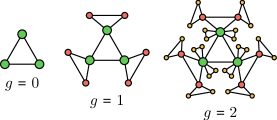
Figure 1: Construction process for the Koch network.

Let $L_{v}(g_{i})$ be the number of nodes generated at iteration $g_{i}$ ($g_{i}\geq 1$). By construction, $L_{v}(g_{i})=6\times 4^{g_{i}-1}$. In $\mathcal{K}_{g}$, the initial three nodes have the largest degree, we thus call them the hub nodes. Let $N_{g}$ and $M_{g}$ denote, respectively, the numbers of nodes and edges in $\mathcal{K}_{g}$. It is easy to derive that $N_{g}=2\times 4^{g}+1$ and $e_{g}=3\times 4^{g}$. Then, the average degree of $\mathcal{K}_{g}$ is $(6\times 4^{g})/(2\times 4^{g}+1)$, which is asymptotically equal to $3$ for large $g$.

The Koch networks display some remarkable characteristics as observed in a large variety of real-world systems [29]. It is scale-free [61], since the degree distribution $P(k)$ follows a power-law behavior $P(k)\sim k^{-3}$. In addition, the Koch networks exhibit the small-world effect [62], since the average geodesic distance grows logarithmically with $N_{g}$ and the average clustering coefficient is high, converging to a nonzero value $0.82$ for large $g$.

6.1.2 Explicit expression for diagonal of pseudoinverse of laplacian

Let $\bm{\mathit{L}}^{\dagger}(g)$ denote the Laplacian matrix of network $\mathcal{K}_{g}$. Let $V_{g}$ denote the set of the $N_{g}$ vertices in the Koch network $\mathcal{K}_{g}$. Let $\bm{\mathit{L}}_{xx}^{\dagger}(g)$ be the diagonal entry of $\bm{\mathit{L}}^{\dagger}(g)$ associated with node $x$. Let $r_{xy}(g)$ denote the resistance distance between two vertices $x$ and $y$ in $\mathcal{K}_{g}$. Then the resistance distance $r_{x}(g)$ of node $x$ in $\mathcal{K}_{g}$ is $r_{x}(g)=\sum_{y\in V_{g}}r_{xy}(g)$. And let $\delta(g)$ denote the Kirchhoff index of $\mathcal{K}_{g}$.

By (8), in order to determine $\bm{\mathit{L}}_{xx}^{\dagger}(g)$, we need first know $\delta(g)$ and $r_{x}(g)$. It was shown [63] that the Kirchhoff index of $\mathcal{K}_{g}$ is

$$\delta(g)=\frac{2^{4g+1}(6g+7)+4^{g+1}}{9}\,.$$ (15)

We now calculate $r_{x}(g)$. Let $d_{xy}(g)$ be the shortest-path distance between a pair of nodes $x$ and $y$ in $\mathcal{K}_{g}$. By construction of Koch networks, we have $r_{xy}(g)=2d_{xy}(g)/3$. Define $d_{x}(g)=\sum_{y\in V_{g}}d_{xy}(g)$ as the shortest-path distance of node $x$, which is the sum of the shortest-path distances from $x$ to all other nodes in $\mathcal{K}_{g}$. Then,

$$r_{x}(g)=\frac{2}{3}d_{x}(g)\,.$$ (16)

Thus, to find $r_{x}(g)$, one can alternatively compute $d_{x}(g)$.

We next calculate $d_{x}(g)$ for any node in $\mathcal{K}_{g}$. For the convenience of description, we distinguish all nodes in $\mathcal{K}_{g}$, by giving a label sequence to every node, such that the nodes with identical label have identical properties, e.g., degree, resistance distance, and so forth. For this purpose, we classify the $N_{g}$ nodes in $\mathcal{K}_{g}$ into $g+1$ different levels, with the $L_{v}(k)$ nodes created at the $k$th iteration belonging to level $k$. By construction, for an arbitrary node $x$ at level $k$, there is a unique shortest path $v_{0}-v_{1}-v_{2}-\cdots-v_{n}-x$ (where $n\leq k-1$), from the nearest hub node $v_{0}$ at level $0$ to node $x$. We call $\{v_{0},v_{1},v_{2},\cdots,v_{n}\}$ the set of ancestors for node $x$ and $v_{n}$ the parent of node $x$. Hence, each of the three hub nodes at level $0$ is the ancestors of $\frac{N_{g}}{3}-1$ nodes, and all other vertices are the descendant nodes of one of the three hub vertices at level $0$.

According to the unique shortest path to the closest hub node, we label each vertex at level $k$ by a unique sequence $\{i_{0},i_{1},i_{2},\cdots,i_{n},k\}$, where $i_{j}$ is the level of node $v_{j}$ on the shortest path. It is easy to see that $i_{0}=0$ and $0<i_{1}<i_{2}<\cdots<i_{n}<k$. Although different nodes may have the same labels, nodes with the same label have the same properties. According to this labeling, for a node having label (sequence) $\{i_{0},i_{1},i_{2},\cdots,i_{n}\}$, its parent has a label $\{i_{0},i_{1},i_{2},\cdots,i_{n-1}\}$, and its ancestors have a label $\{i_{0},i_{1},i_{2},\cdots,i_{k}\}$, where $k=0,1,\cdots,n-1$.

As shown above, for any node $x$ in $\mathcal{K}_{g}$ it has a unique label $\{i_{0},i_{1}\cdots,i_{n}\}$, where $i_{0}=0$ and $0<i_{1}<i_{2}<\cdots<i_{n}\leq g$, and for any pair of different vertices with identical labels, the value $d_{x}(g)$, or alternatively represented by $d_{\{i_{0},i_{1},\cdots,i_{n}\}}(g)$, for the two nodes is also identical. Based on the particular construction of $\mathcal{K}_{g}$, we can derive an explicit expression for $d_{x}(g)$ for any node $x$, as stated in the following lemma.

Lemma 6.1.

For a node $x$ in the Koch networks $\mathcal{K}_{g}$ with label $\{i_{0},i_{1},\cdots,i_{n}\}$, its shortest-path distance is

$$d_{\{i_{0},i_{1},\cdots,i_{n}\}}(g)=(g+2)4^{g}+2n\cdot 4^{g}-\sum_{k=1}^{n}2\cdot 4^{g-i_{k}}\,.$$ (17)

Proof 6.2.

By construction, for any node $x$ with label $\{0,i_{1},i_{2},\cdots,i_{n}\}$ at level $i_{n}$, there exists another vertex $x^{\prime}$, called brother of $x$. These two brothers are generated simultaneously, both of which and their parent, denoted $p$, form a triangle. It is easy to see that the label of $p$ is $\{0,i_{1},i_{2},\cdots,i_{n-1}\}$. To prove the lemma, we first derive the recursive relation between $d_{\{0,i_{1},i_{2},\cdots,i_{n}\}}(g)$ for node $x$ and $d_{\{0,i_{1},i_{2},\cdots,i_{n-1}\}}(g)$ for its parent $p$.

Note that among the $N_{g}$ nodes in $\mathcal{K}_{g}$, $N_{g-i_{n}}/3$ nodes (including node $x$) are the descendants of $x$, which constitute a set $V^{x}_{g}$; $N_{g-i_{n}}/3$ nodes (containing node $x^{\prime}$) are the descendants of node $x^{\prime}$, which form a set $V^{x^{\prime}}_{g}$; and the remaining $N_{g}-(2N_{g-i_{n}}/3)$ nodes form a set $V^{p}_{g}$. Then, $V_{g}=V^{x}_{g}\bigcup V^{x^{\prime}}_{g}\bigcup V^{p}_{g}$ and $V^{x}_{g}\bigcap V^{x^{\prime}}_{g}\bigcap V^{p}_{g}=\emptyset$. By definition, for a node $y\in V^{x}_{g}$, $d_{xy}(g)=d_{py}(g)-1$; for a node $j\in V^{x^{\prime}}_{g}$, $d_{xy}(g)=d_{py}(g)$; and for a node $y\in V^{p}_{g}$, $d_{xy}(g)=d_{py}(g)+1$. Thus

$$d_{x}(g)=d_{\{0,i_{1},i_{2},\cdots,i_{n}\}}(g)=\sum_{y\in V_{g}}{d_{xy}(g)}$$

$$= \sum_{y\in V^{x}_{g}}{d_{xy}(g)}+\sum_{y\in V^{x^{\prime}}_{g}}{d_{xy}(g)}+\sum_{y\in V^{p}_{g}}{d_{xy}(g)}$$

$$= \sum_{y\in V^{x}_{g}}(d_{py}(g)-1)+\sum_{y\in V^{x^{\prime}}_{g}}{d_{py}(g)}+\sum_{y\in V^{p}_{g}}(d_{py}(g)+1)$$

$$= \sum_{y\in V^{x}_{g}}d_{py}(g)-\frac{1}{3}N_{g-i_{n}}+\sum_{y\in V^{x^{\prime}}_{g}}{d_{py}(g)}+\sum_{j\in V^{p}_{g}}d_{py}(g)$$

$$\quad+N_{g}-\frac{2}{3}N_{g-i_{n}}$$

$$= \sum_{y\in V_{g}}{d_{py}(g)}+N_{g}-N_{g-i_{n}}$$

$$= d_{p}(g)+N_{g}-N_{g-i_{n}}$$

$$= d_{\{0,i_{1},i_{2},\cdots,i_{n-1}\}}(g)+2\cdot 4^{g}-2\cdot 4^{g-i_{n}}\,.$$ (18)

Repeatedly applying (18), we obtain

$$d_{\{0,i_{1},i_{2},\cdots,i_{n}\}}(g)$$

$$= d_{\{0,i_{1},i_{2},\cdots,i_{n-1}\}}(g)+2\cdot 4^{g}-2\cdot 4^{g-i_{n}}$$

$$= d_{\{0,i_{1},i_{2},\cdots,i_{n-2}\}}(g)+4\cdot 4^{g}-2\cdot 4^{g-i_{n-1}}-2\cdot 4^{g-i_{n}}$$

$$= \cdots$$

$$= d_{\{0\}}(g)+2n\cdot 4^{g}-\sum_{k=1}^{n}2\cdot 4^{g-i_{k}}$$

$$= (g+2)4^{g}+2n\cdot 4^{g}-\sum_{k=1}^{n}2\cdot 4^{g-i_{k}}\,,$$ (19)

where $d_{\{0\}}(g)=(g+2)4^{g}$ derived in [30] was used.

We note that Lemma 17 was previously given in [64], where the proof is omitted. Then, the resistance distance of a node in $\mathcal{K}_{g}$ can be directly determined by plugging (17) to (16).

Lemma 6.3.

In the Koch networks $\mathcal{K}_{g}$, the resistance distance of node $x$ labelled by $\{i_{0},i_{1},\cdots,i_{n}\}$ is

$$r_{x}(g)=\frac{2\times[(g+2)4^{g}+2n\cdot 4^{g}-\sum_{k=1}^{n}2\cdot 4^{g-i_{k}}]}{3}\,.$$ (20)

Inserting (15) and (20) into (8), we obtain an exact expression for $\bm{\mathit{L}}^{\dagger}_{xx}(g)$ associated with any node in $\mathcal{K}_{g}$.

Theorem 6.4.

For the Koch network $\mathcal{K}_{g}$, the diagonal entry $\bm{\mathit{L}}^{\dagger}_{xx}(g)$ corresponding to node $x$ with label $\{i_{0},i_{1},\cdots,i_{n}\}$ is

$$\bm{\mathit{L}}^{\dagger}_{xx}(g) =\frac{2}{3(2\cdot 4^{g}+1)^{2}}\left(2n\cdot 4^{g}-\displaystyle\sum_{k=1}^{n}2\cdot 4^{g-i_{k}}\right)$$

$$\quad+\frac{2^{2g+1}(5\cdot 4^{g}+3g+4)}{9(2\cdot 4^{g}+1)^{2}}.$$ (21)

6.1.3 Ordering of nodes by diagonal of pseudoinverse for laplacian

Besides the explicit expression for the diagonal entries of pseudoinverse for Laplacian matrix, we can also compare the diagonal entries for any pair of nodes in $\mathcal{K}_{g}$.

Theorem 6.5.

For two different nodes $x_{i}$ and $x_{j}$ in $\mathcal{K}_{g}$, with their labels being, respectively, $\{i_{0},i_{1},\cdots,i_{n_{i}}\}$ and $\{j_{0},j_{1},\cdots,j_{n_{j}}\}$ where $i_{0}=j_{0}=0$,

1. if $n_{i}>n_{j}$, then $\bm{\mathit{L}}^{\dagger}_{x_{i}x_{i}}(g)>\bm{\mathit{L}}^{\dagger}_{x_{j}x_{j}}(g)$;

2. if $n_{i}<n_{j}$, then $\bm{\mathit{L}}^{\dagger}_{x_{i}x_{i}}(g)<\bm{\mathit{L}}^{\dagger}_{x_{j}x_{j}}(g)$;

3. if $n_{i}=n_{j}$, and

   1. if there exists a natural integer $z$ with $0\leqslant z\leqslant n_{i}$, such that $i_{l}=j_{l}$ for $l=0,1,2,\cdots,z-1$, but $i_{z}\neq j_{z}$,

      1. if $i_{z}>j_{z}$, then $\bm{\mathit{L}}^{\dagger}_{x_{i}x_{i}}(g)>\bm{\mathit{L}}^{\dagger}_{x_{j}x_{j}}(g)$;

      2. if $i_{z}<j_{z}$, then $\bm{\mathit{L}}^{\dagger}_{x_{i}x_{i}}(g)<\bm{\mathit{L}}^{\dagger}_{x_{j}x_{j}}(g)$;

   2. if $i_{l}=j_{l}$ for $l=0,1,2,\cdots,n_{i}$, then $\bm{\mathit{L}}^{\dagger}_{x_{i}x_{i}}(g)=\bm{\mathit{L}}^{\dagger}_{x_{j}x_{j}}(g)$.

Proof 6.6.

Equality (8) implies that the ordering of nodes by $\bm{\mathit{L}}^{\dagger}_{xx}$ is consistent with the ordering of nodes by resistance distance $r_{x}(g)$. On the other hand, the ordering of nodes by resistance distance $r_{x}(g)$ agrees with the the ordering of nodes by shortest-path distance $d_{x}(g)$. For any pair of nodes $x_{i}$ and $x_{j}$, in order to compare $\bm{\mathit{L}}^{\dagger}_{x_{i}x_{i}}(g)$ and $\bm{\mathit{L}}^{\dagger}_{x_{j}x_{j}}(g)$, we can alternatively compare $d_{x_{i}}(g)$ and $d_{x_{j}}(g)$.

According to (17), we have

$$\begin{split}&\quad d_{x_{i}}(g)-d_{x_{j}}(g)\\ &=d_{\{0,i_{1},i_{2},\cdots,i_{n_{i}}\}}(g)-d_{\{0,j_{1},j_{2},\cdots,j_{n_{j}}\}}(g)\\ &=2\cdot 4^{g}(n_{i}-n_{j})-\sum_{k=1}^{n_{i}}2\cdot 4^{g-i_{k}}+\sum_{k=1}^{n_{j}}2\cdot 4^{g-j_{k}}.\end{split}$$ (22)

We can compare $d_{x_{i}}(g)$ and $d_{x_{j}}(g)$ by distinguishing three cases.

1. Case I: $n_{i}>n_{j}$. In this case, it is obvious that $n_{i}-n_{j}\geqslant 1$. Moreover, $g\geqslant n_{i}>n_{j}\geqslant 1$. Then, we get

   $$\begin{split}&\quad d_{x_{i}}(g)-d_{x_{j}}(g)\\ &=2\cdot 4^{g}(n_{i}-n_{j})-\sum_{k=1}^{n_{i}}2\cdot 4^{g-i_{k}}+\sum_{k=1}^{n_{j}}2\cdot 4^{g-j_{k}}\\ &>2\cdot 4^{g}-2\,\sum_{k=0}^{g-1}4^{k}=2\cdot 4^{g}-\frac{2}{3}(4^{g}-1)>0\,,\end{split}$$ (23)

   which means $d_{x_{i}}(g)>d_{x_{j}}(g)$ and thus $\bm{\mathit{L}}^{\dagger}_{x_{i}x_{i}}(g)>\bm{\mathit{L}}^{\dagger}_{x_{j}x_{j}}(g)$.

2. Case II: $n_{i}<n_{j}$. For this case, we can prove $\bm{\mathit{L}}^{\dagger}_{x_{i}x_{i}}(g)<\bm{\mathit{L}}^{\dagger}_{x_{j}x_{j}}(g)$, by using a process similar to the first case $n_{i}>n_{j}$.

3. Case III: $n_{i}=n_{j}$. For this particular case, we distinguish two subcases.

   1. If there exists a positive integer $z$ ($0<z\leqslant n_{i}$), such that $i_{l}=j_{l}$ for $l=0,1,2,\cdots,z-1$, but $i_{z}\neq j_{z}$, then

      $$\begin{split}&\quad d_{x_{i}}(g)-d_{x_{j}}(g)\\ &=2\cdot 4^{g}(n_{i}-n_{j})-\sum_{k=1}^{n_{i}}2\cdot 4^{g-i_{k}}+\sum_{k=1}^{n_{j}}2\cdot 4^{g-j_{k}}\\ &=2\left(-\sum_{k=z}^{n_{i}}4^{g-i_{k}}+\sum_{k=z}^{n_{j}}4^{g-j_{k}}\right).\end{split}$$ (24)

      1. If $i_{z}>j_{z}$, then

         $$\begin{split}&\quad d_{x_{i}}(g)-d_{x_{j}}(g)\\ &\geqslant 6\cdot 4^{g-i_{z}}-2\sum_{k=0}^{g-i_{z}-1}4^{k}>\frac{16}{3}\cdot 4^{g-i_{z}}>0\,,\end{split}$$ (25)

         which implies $\bm{\mathit{L}}^{\dagger}_{x_{i}x_{i}}(g)>\bm{\mathit{L}}^{\dagger}_{x_{j}x_{j}}(g)$.

      2. If $i_{z}<j_{z}$, we can analogously prove that $\bm{\mathit{L}}^{\dagger}_{x_{i}x_{i}}(g)<\bm{\mathit{L}}^{\dagger}_{x_{j}x_{j}}(g)$.

   2. If $i_{l}=j_{l}$ holds for $l=0,1,2,\cdots,n_{i}$, it is easy to prove that $\bm{\mathit{L}}^{\dagger}_{x_{i}x_{i}}(g)=\bm{\mathit{L}}^{\dagger}_{x_{j}x_{j}}(g)$.

This completes the proof.

Since the diagonal entry of $\bm{\mathit{L}}^{\dagger}(g)$ is consistent with the structural centrality, current flow centrality, and information centrality of nodes in Koch networks $\mathcal{K}_{g}$, Theorem 6.5 shows that ranking nodes in $\mathcal{K}_{g}$ according to the values of diagonal for $\bm{\mathit{L}}^{\dagger}(g)$ captures the information of all the three centralities for all nodes in $\mathcal{K}_{g}$.

6.2 Diagonal of Pseudoinverse of Laplacian for Uniform Recursive Trees

This subsection is devoted to determining the diagonal entries for the pseudoinverse of Laplacian for uniform recursive trees [31], which are also constructed in an iterative way. Let $\mathcal{U}_{g}$ ($g\geq 0$) be the networks after $g$ iterations. For $g=0$, $\mathcal{U}_{0}$ contains an isolated node, called the central node. For $g=1$, $f$ ($f$ is a positive natural number) new nodes are created and linked to the central node to form $\mathcal{U}_{1}$. For $g\geq 1$, $\mathcal{U}_{g}$ is obtained from $\mathcal{U}_{g-1}$ by performing the following operations: For each node in $U_{g-1}$, $f$ new nodes are generated and attached to it. Figure 2 illustrates the first several iterative constructions of a particular network for $f=3$.

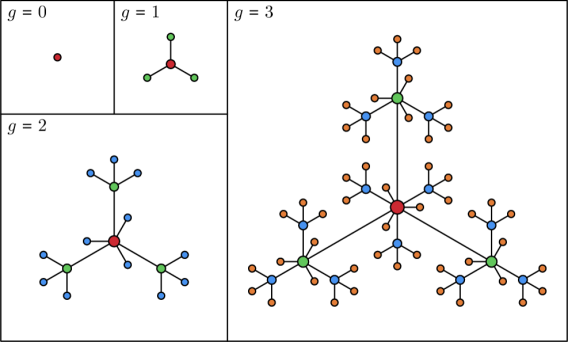
Figure 2: Construction process of a special network for $f=3$.

In the case without inducing confusion, we use the same notations as those for Koch networks. By construction, at each iterative step $g_{i}$ ($g_{i}\geq 1$), the number of newly generated nodes is $L({g_{i}})=f{(f+1)^{{g_{i}}-1}}$. Then in network $\mathcal{U}_{g}$, there are $N_{g}=(f+1)^{g}$ nodes and ${E_{g}}={(f+1)^{g}}-1$ edges. In contrast to Koch networks, the uniform recursive trees are not scale-free, but have an exponential form degree distribution. It has been observed [51] that the degree distribution of some real-world networks also decays exponentially, such as power grid. In addition, the uniform recursive trees are small-world with a low average shortest distance.

The special construction of the uniform recursive trees allows to determine exactly relevant quantities. It was shown [31] that the Kirchhoff index of $\mathcal{U}_{g}$ is

$$\delta(g)=(fg-1)(f+1)^{2g-1}+(f+1)^{g-1}\,.$$ (26)

We next determine the diagonal $\bm{\mathit{L}}_{xx}^{\dagger}(g)$ of the pseudoinverse $\bm{\mathit{L}}_{xx}(g)$ for the Laplacian matrix for graph $\mathcal{U}_{g}$, based on the relation in (8). To do so, we need first find $r_{x}(g)$ Note that for $\mathcal{U}_{g}$, $r_{ij}(g)=d_{ij}(g)$ for any pair of nodes, due to the tree-like structure.

In order to determine $r_{x}(g)$, similar to that of Koch networks, we classify the $N_{g}$ nodes in $\mathcal{U}_{g}$ into $g+1$ different levels, based on which we provide a label to each node in $\mathcal{U}_{g}$. For any node $x$ in $\mathcal{U}_{g}$, we label it by a sequence of node level information $\{0,i_{1},i_{2},...,i_{n}\}$, $0<i_{1}<i_{2}<...<i_{n}\leq g$. For any node $x$ with labeling $\{0,i_{1},i_{2},...,i_{n}\}$, we interchangeably use $x$ or $\{0,i_{1},i_{2},...,i_{n}\}$ to represent this node. For example, for the central node at level $0$ in $\mathcal{U}_{g}$, its resistance distance can be written as $r_{\{0\}}(g)$.

Before determining $r_{x}(g)$ for an arbitrary node $x$, we first we calculate $r_{\{0\}}(g)$. For $g=1$, $r_{\{0\}}(1)=f$. For $g>1$, $r_{\{0\}}(g)$ satisfies the following recursion relation.

$$r_{\{0\}}(g)=r_{\{0\}}(g-1)+f\left(r_{\{0\}}(g-1)+N_{g-1}\right),$$

which under the initial condition $r_{\{0\}}(1)=f$ is solved to yield

$$r_{\{0\}}(g)=g\,f(f+1)^{g-1}.$$ (27)

We are now in position to calculate $r_{x}(g)$ for any node $x$ in $\mathcal{U}_{g}$. Note that for any node $x$ with label $\{0,i_{1},i_{2},...,i_{n}\}$, $0<i_{1}<i_{2}<...<i_{n}\leq g$, its parent, denoted by $p$, has a label $\{0,i_{1},i_{2},...,i_{n-1}\}$. We can derive the relation between $r_{\{0,i_{1},i_{2},...,i_{n}\}}(g)$ and $r_{\{0,i_{1},i_{2},...,i_{n-1}\}}(g)$. Notice that the descendants of node $x$ at level $i_{n}$ and $x$ itself constitute one subunit of the whole network $\mathcal{U}_{g}$, which is a copy of $\mathcal{U}_{g-i_{n}}$. The node number of this subunit is $N_{g-i_{n}}$. Let $\Omega$ denote the set of nodes in $\mathcal{U}_{g}$, and let $\Omega_{x}$ denote the set of the descendant nodes of $x$. Then, $\Omega=\Omega_{x}\bigcup\overline{\Omega}_{x}$. By construction, for any node $y\in\Omega_{x}$, $r_{xy}(g)=r_{py}(g)-1$. While for any node $y\in\overline{\Omega}_{x}$, $r_{xy}(g)=r_{py}(g)+1$. Thus

$$\quad r_{\{0,i_{1},i_{2},...,i_{n}\}}(g)=r_{x}(g)=\sum_{y\in\Omega}{r_{xy}(g)}$$

$$=\sum_{y\in\Omega_{x}}{r_{xy}(g)}+\sum_{y\in\overline{\Omega}_{x}}{r_{xy}(g)}$$

$$=\sum_{y\in\Omega_{x}}{(r_{py}(g)-1)}+\sum_{y\in\overline{\Omega}_{x}}{(r_{py}(g)+1)}$$

$$=\sum_{y\in\Omega_{x}}{r_{py}(g)}-N_{g-i_{n}}+\sum_{y\in\overline{\Omega}_{x}}{r_{py}(g)}+N_{g}-N_{g-i_{n}}$$

$$=\sum_{y\in\Omega}{r_{py}(g)}+N_{g}-2N_{g-i_{n}}$$

$$=r_{p}(g)+N_{g}-2N_{g-i_{n}}$$

$$=r_{\{0,i_{1},i_{2},...,i_{n-1}\}}(g)+(f+1)^{g}-2(f+1)^{g-i_{n}}.$$

Using the above relation (LABEL:RSX2) repeatedly to give

$$\quad r_{\{0,i_{1},i_{2},...,i_{n}\}}(g)$$

$$=r_{\{0,i_{1},i_{2},...,i_{n-1}\}}(g)+\left[(f+1)^{g}-2(f+1)^{g-i_{n}}\right]$$

$$=r_{\{0,i_{1},i_{2},...,i_{n-2}\}}(g)+\left[(f+1)^{g}-2(f+1)^{g-i_{n-1}}\right]$$

$$\quad+\left[(f+1)^{g}-2(f+1)^{g-i_{n}}\right]$$

$$=\cdots\cdots$$

$$=r_{\{0\}}(g)+\sum_{k=1}^{n}\left[(f+1)^{g}-2(f+1)^{g-i_{k}}\right],$$ (29)

which, together with $r_{\{0\}}(g)=g\,f(f+1)^{g-1}$, is solved to obtain the following result.

Lemma 6.7.

For a node $x$ in the uniform recursive tree $\mathcal{U}_{g}$ with label $\{i_{0},i_{1},\cdots,i_{n}\}$, its resistance distance is

$$\quad r_{x}(g)=r_{\{0,i_{1},i_{2},...,i_{n}\}}(g)$$

$$=gf(f+1)^{g-1}+(f+1)^{g}[n-2\sum_{k=1}^{n}(f+1)^{-i_{k}}]\,.$$ (30)

Plugging (26) and (6.7) into (8) yields an explicit expression for $\bm{\mathit{L}}^{\dagger}_{xx}(g)$ associated with any node in $\mathcal{U}_{g}$.

Theorem 6.8.

For Laplacian matrix $\bm{\mathit{L}}(g)$ of the uniform recursive tree $\mathcal{U}_{g}$, the diagonal entry $\bm{\mathit{L}}^{\dagger}_{xx}(g)$ of its pseudoinverse $\bm{\mathit{L}}^{\dagger}(g)$ corresponding to node $x$ with label $\{i_{0},i_{1},\cdots,i_{n}\}$ is given by

$$\bm{\mathit{L}}^{\dagger}_{xx}(g)=n-2\sum_{k=1}^{n}(f+1)^{-i_{k}}+\frac{1}{f+1}-(f+1)^{-(g+1)}.$$ (31)

In addition to the exact expression for the diagonal of $\bm{\mathit{L}}^{\dagger}(g)$ for $\mathcal{U}_{g}$, one can also compare the diagonal entries between any two nodes in $\mathcal{U}_{g}$ with $f\geq 2$, as stated in the following theorem.

Theorem 6.9.

In the case of $f\geq 2$, for two different nodes $x_{i}$ and $x_{j}$ in the uniform recursive tree $\mathcal{U}_{g}$, with their labels being, respectively, $\{i_{0},i_{1},\cdots,i_{n_{i}}\}$ and $\{j_{0},j_{1},\cdots,j_{n_{j}}\}$ where $i_{0}=j_{0}=0$,

1. if $n_{i}>n_{j}$, then $\bm{\mathit{L}}^{\dagger}_{x_{i}x_{i}}(g)>\bm{\mathit{L}}^{\dagger}_{x_{j}x_{j}}(g)$.

2. if $n_{i}<n_{j}$, then $\bm{\mathit{L}}^{\dagger}_{x_{i}x_{i}}(g)<\bm{\mathit{L}}^{\dagger}_{x_{j}x_{j}}(g)$.

3. if $n_{i}=n_{j}$, and

   1. if there exists a natural integer $z$ with $0\leqslant z\leqslant n_{i}$, such that $i_{l}=j_{l}$ for $l=0,1,2,\cdots,z-1$, but $i_{z}\neq j_{z}$,

      1. if $i_{z}>j_{z}$, then $\bm{\mathit{L}}^{\dagger}_{x_{i}x_{i}}(g)>\bm{\mathit{L}}^{\dagger}_{x_{j}x_{j}}(g)$;

      2. if $i_{z}<j_{z}$, then $\bm{\mathit{L}}^{\dagger}_{x_{i}x_{i}}(g)<\bm{\mathit{L}}^{\dagger}_{x_{j}x_{j}}(g)$;

   2. if $i_{l}=j_{l}$ for $l=0,1,2,\cdots,n_{i}$, then $\bm{\mathit{L}}^{\dagger}_{x_{i}x_{i}}(g)=\bm{\mathit{L}}^{\dagger}_{x_{j}x_{j}}(g)$.

We omit the proof of Theorem 6.9, since it is similar to that for Theorem 6.5.

7 Numerical Results On Model Networks

To further demonstrate the performance of our approximation algorithm $\text{Approx}\mathcal{D}$, we use it to compute the diagonal elements of pseudoinverse of Laplacian matrix for some model networks, as well as their Kirchhoff index.

7.1 Diagonal of Pseudoinverse for Laplacian

We first apply our algorithm $\text{Approx}\mathcal{D}$ to approximately compute the diagonal elements of pseudoinverse of Laplacian matrix for the Koch network $\mathcal{K}_{10}$ and uniform recursive tree $\mathcal{U}_{11}$ with $f=3$. Let $V$ be the set of nodes in these two graphs. Table 4 reports the maximum relative error $\sigma_{\max}=\max_{u\in V}|\bm{\mathit{L}}^{\dagger}_{uu}-\tilde{\bm{\mathit{L}}}^{\dagger}_{uu}|/{\bm{\mathit{L}}^{\dagger}_{uu}}$, mean relative error $\sigma=\frac{1}{|V|}\sum_{u\in V}|\bm{\mathit{L}}^{\dagger}_{uu}-\tilde{\bm{\mathit{L}}}^{\dagger}_{uu}|/{\bm{\mathit{L}}^{\dagger}_{uu}}$, and running time of our numerical results.

Table 4: Maximum relative error, mean relative error, and running time (seconds, $s$) for $\tilde{\mathcal{L}^{\dagger}}$ on networks $\mathcal{K}_{10}$ and $\mathcal{U}_{11}$ with $f=3$. The diagonal elements of $\bm{\mathit{L}}^{\dagger}(g)$ are obtained via (6.4) and (31), while $\tilde{\mathcal{L}^{\dagger}}$ is obtained through algorithm $\mathtt{Approx\mathcal{D}}$ with $\epsilon=0.1$.

Network	Vertices	Edges	$\sigma_{\max}$	$\sigma$	Time
$K_{10}$	2,097,153	3,145,728	0.1366	0.0225	1630
$U_{11}$	4,194,304	4,194,303	0.1401	0.0220	4496

7.2 Kirchhoff Index

We proceed to present our numerical results for Kirchhoff index of three model networks, including Koch networks, uniform recursive trees, and pseudofractal scale-free webs [32, 33, 65]. For the first two graphs, the exact results for Kirchhoff index have been obtained in the previous section, given by (15) and (26), respectively. Hence we only need to determine the Kirchhoff index for pseudofractal scale-free webs.

Let $\mathcal{F}_{g}$ ($g\geq 0$) denote the pseudofractal scale-free webs after $g$ iterations. For $g=0$, $\mathcal{F}_{0}$ includes a triangle of three nodes and three edges. For $g>0$, $\mathcal{F}_{g}$ is obtained from $\mathcal{F}_{g-1}$ in the following way. For each existing edge in $\mathcal{F}_{g-1}$, a new node is created and connected to both end nodes of the edge. Figure 3 schematically illustrates the construction process of the graph. In $\mathcal{F}_{g}$, there are $(3^{g+1}+3)/2$ nodes and $3^{g+1}$ edges. Like the Koch networks, the pseudofractal scale-free webs also exhibit the striking scale-free small-world properties of many real networks. It has been shown [66, 28] that the Kirchhoff index $\delta(g)$ for $\mathcal{F}_{g}$ is

$$\delta(g) =\frac{1}{112}\cdot\frac{1}{3^{g+2}}\times$$

$$\quad\big{(}50\cdot 3^{3g+3}-35\cdot 3^{2g+2}2^{g+1}+48\cdot 3^{2g+2}$$

$$\quad+30\cdot 3^{g+2}2^{g+1}-14\cdot 3^{g+2}+225\cdot 2^{g+1}\big{)}\,.$$ (32)

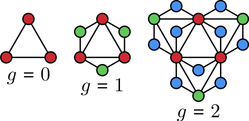
Figure 3: Iterative construction process of the pseudofractal scale-free webs.

Table 5 reports our numerical results for Kirchhoff index on three model networks, $\mathcal{K}_{10}$, $\mathcal{U}_{11}$ with $f=3$, and $\mathcal{F}_{12}$. All these numerical results are obtained via algorithm $\text{Approx}\mathcal{D}$.

Table 5: Exact Kirchhoff index $\delta$, their approximation $\tilde{\delta}$, relative error $\rho=(\delta-\tilde{\delta})/\delta$, and running time (seconds, $s$) for $\tilde{\delta}$ on three networks, $\mathcal{K}_{10}$, $\mathcal{U}_{11}$ with $f=3$, and $\mathcal{F}_{12}$. $\delta$ is obtained via (15), (26), and (7.2), while $\tilde{\delta}$ is obtained through algorithm $\text{Approx}\mathcal{D}$ with $\epsilon=0.1$.

Net	Vertices	Edges	$\delta$	$\tilde{\delta}$	$\rho$ ($\times 10^{-3}$)	Time
$K_{10}$	2,097,153	3,145,728	140,737,489,403,904	140,679,655,505,316	0.4109346	4496
$U_{11}$	4,194,304	4,194,303	3,396,122,345,421	3,396,602,496,861	0.1413823	1155
$\mathcal{F}_{13}$	2,097,153	3,145,728	16,370,506,924,032	16,346,238,029,818	1.4824766	1630

Tables 4 and 5 show that the approximation algorithm $\text{Approx}\mathcal{D}$ works effectively for all studied model networks. This again demonstrates the advantage of our proposed algorithm for large-scale networks.

8 Conclusions

The problem of estimating the diagonal entries of pseudoinverse $\bm{\mathit{L}}^{\dagger}$ of the Laplacian matrix associated with a graph arises in various applications ranging from network science to social networks and control science. In this paper, we presented an inexpensive technique to approximately compute all the diagonal entries of $\bm{\mathit{L}}^{\dagger}$ for a weighted undirected graph. Our method is based on the Johnson-Lindenstrauss Lemma and nearly-linear time solver, and has nearly linear time computation complexity. We analytically demonstrated that the approximation algorithm provides an approximation guarantee with error bounds. Moreover, we determined exactly all the diagonal entries of the pseudoinverse $\bm{\mathit{L}}^{\dagger}(g)$ the Laplacian matrices for two iteratively growing networks, the scale-free small-world Koch networks and the uniform recursive trees. With the help of several recursive relations derived from the particular structure of the two networks, we obtained rigorous expressions for every entry of matrix $\bm{\mathit{L}}^{\dagger}(g)$. We conducted extensive numerical experiments on various real-world networks and three model networks, the results of which demonstrate that the proposed approximation method is both effective and efficient. In future work, we plan to study nearly-linear time algorithm estimating the diagonal entries of pseudoinverse for a directed graph Laplacian [67], by using the approach of sparse LU factorizations developed in [68].

References

- [1] Merris, R. (1994) Laplacian matrices of graphs: A survey. Linear Algebra and its Applications, 197, 143–176.
- [2] Kirkland, S. (2018) The group inverse of the Laplacian matrix of a graph. Combinatorial Matrix Theory, pp. 131–171. Springer.
- [3] Sarkar, P. and Moore, A. W. (2011) Random walks in social networks and their applications: A survey. Social Network Data Analytics, pp. 43–77. Springer.
- [4] Dörfler, F., Simpson-Porco, J. W., and Bullo, F. (2018) Electrical networks and algebraic graph theory: Models, properties, and applications. Proceedings of the IEEE, 106, 977–1005.
- [5] Estrada, E. and Hatano, N. (2010) A vibrational approach to node centrality and vulnerability in complex networks. Physica A, 389, 3648–3660.
- [6] Ranjan, G. and Zhang, Z.-L. (2011) A geometric approach to robustness in complex networks. Proceedings of 2011 31st International Conference on Distributed Computing Systems Workshops, pp. 146–153. IEEE.
- [7] Ranjan, G. and Zhang, Z.-L. (2013) Geometry of complex networks and topological centrality. Physica A, 392, 3833–3845.
- [8] Van Mieghem, P., Devriendt, K., and Cetinay, H. (2017) Pseudoinverse of the Laplacian and best spreader node in a network. Physical Review E, 96, 032311.
- [9] Siami, M., Bamieh, B., Bolouki, S., and Motee, N. (2016) Notions of centrality in consensus protocols with structured uncertainties. Proceedings of 2016 IEEE 55th Conference on Decision and Control, pp. 3542–3547. IEEE.
- [10] Siami, M., Bolouki, S., Bamieh, B., and Motee, N. (2018) Centrality measures in linear consensus networks with structured network uncertainties. IEEE Transactions on Control of Network Systems, 5, 924–934.
- [11] Klein, D. J. and Randić, M. (1993) Resistance distance. Journal of Mathematical Chemistry, 12, 81–95.
- [12] Tizghadam, A. and Leon-Garcia, A. (2010) Autonomic traffic engineering for network robustness. IEEE Journal on Selected Areas in Communications, 28.
- [13] Li, H. and Zhang, Z. (2018) Kirchhoff index as a measure of edge centrality in weighted networks: Nearly linear time algorithms. Proceedings of the 29th Annual ACM-SIAM Symposium on Discrete Algorithms, pp. 2377–2396.
- [14] Patterson, S. and Bamieh, B. (2014) Consensus and coherence in fractal networks. IEEE Transactions on Control of Network Systems, 1, 338–348.
- [15] Shi, X., Cao, J., and Huang, W. (2018) Distributed parametric consensus optimization with an application to model predictive consensus problem. IEEE Trans. Cybern., 48, 2024–2035.
- [16] Su, H., Ye, Y., Qiu, Y., Cao, Y., and Chen, M. Z. (2019) Semi-global output consensus for discrete-time switching networked systems subject to input saturation and external disturbances. IEEE Trans. Cybern., 49, 3934–3945.
- [17] Su, H., Liu, Y., and Zeng, Z. (2020) Second-order consensus for multiagent systems via intermittent sampled position data control. IEEE Trans. Cybern., 50, 2063–2072.
- [18] Fitch, K. and Leonard, N. E. (2016) Joint centrality distinguishes optimal leaders in noisy networks. IEEE Transactions on Control of Network Systems, 3, 366–378.
- [19] Li, H., Peng, R., Shan, L., Yi, Y., and Zhang, Z. (2019) Current flow group closeness centrality for complex networks. Proceedings of World Wide Web Conference, pp. 961–971. ACM.
- [20] Poulakakis, I., Young, G. F., Scardovi, L., and Leonard, N. E. (2016) Information centrality and ordering of nodes for accuracy in noisy decision-making networks. IEEE Transactions on Automatic Control, 61, 1040–1045.
- [21] Ghosh, A., Boyd, S., and Saberi, A. (2008) Minimizing effective resistance of a graph. SIAM Review, 50, 37–66.
- [22] Ranjan, G., Zhang, Z.-L., and Boley, D. (2014) Incremental computation of pseudo-inverse of Laplacian. Proceedins of International Conference on Combinatorial Optimization and Applications, pp. 729–749. Springer.
- [23] Bozzo, E. and Franceschet, M. (2012) Approximations of the generalized inverse of the graph Laplacian matrix. Internet Mathematics, 8, 456–481.
- [24] Tang, J. M. and Saad, Y. (2011) Domain-decomposition-type methods for computing the diagonal of a matrix inverse. SIAM Journal on Scientific Computing, 33, 2823–2847.
- [25] Tang, J. M. and Saad, Y. (2012) A probing method for computing the diagonal of a matrix inverse. Numerical Linear Algebra with Applications, 19, 485–501.
- [26] Wu, L., Laeuchli, J., Kalantzis, V., Stathopoulos, A., and Gallopoulos, E. (2016) Estimating the trace of the matrix inverse by interpolating from the diagonal of an approximate inverse. Journal of Computational Physics, 326, 828–844.
- [27] Qi, Y., Zhang, Z., Yi, Y., and Li, H. (2019) Consensus in self-similar hierarchical graphs and Sierpiński graphs: Convergence speed, delay robustness, and coherence. IEEE Trans. Cybern., 49, 592–603.
- [28] Yi, Y., Zhang, Z., and Patterson, S. (2020) Scale-free loopy structure is resistant to noise in consensus dynamics in power-law graphs. IEEE Trans. Cybern., 51, 190–200.
- [29] Newman, M. E. J. (2003) The structure and function of complex networks. SIAM Review, 45, 167–256.
- [30] Zhang, Z., Zhou, S., Xie, W., Chen, L., Lin, Y., and Guan, J. (2009) Standard random walks and trapping on the Koch network with scale-free behavior and small-world effect. Phys. Rev. E, 79, 061113.
- [31] Liu, H. and Zhang, Z. (2013) Laplacian spectra of recursive treelike small-world polymer networks: Analytical solutions and applications. Journal of Chemical Physics, 138, 114904.
- [32] Dorogovtsev, S. N., Goltsev, A. V., and Mendes, J. F. F. (2002) Pseudofractal scale-free web. Phys. Rev. E, 65, 066122.
- [33] Shan, L., Li, H., and Zhang, Z. (2017) Domination number and minimum dominating sets in pseudofractal scale-free web and Sierpiński graph. Theoret. Comput. Sci., 677, 12–30.
- [34] Chebotarev, P. Y. and Shamis, E. V. (1998) On proximity measures for graph vertices. Automation and Remote Control, 59, 1443–1459.
- [35] Doyle, P. G. and Snell, J. L. (1984) Random Walks and Electric Networks. Mathematical Association of America.
- [36] Tetali, P. (1991) Random walks and the effective resistance of networks. Journal of Theoretical Probability, 4, 101–109.
- [37] Brandes, U. and Fleischer, D. (2005) Centrality measures based on current flow. Proceedings of Annual Symposium on Theoretical Aspects of Computer Science, pp. 533–544.
- [38] Stephenson, K. and Zelen, M. (1989) Rethinking centrality: Methods and examples. Social Networks, 11, 1–37.
- [39] Shan, L., Yi, Y., and Zhang, Z. (2018) Improving information centrality of a node in complex networks by adding edges, . pp. 3535–3541.
- [40] Barrat, A., Barthelemy, M., Pastor-Satorras, R., and Vespignani, A. (2004) The architecture of complex weighted networks. Proceedings of the National Academy of Sciences of the United States of America, 101, 3747–3752.
- [41] Li, H. and Schild, A. (2018) Spectral subspace sparsification. Proceedings of 2018 IEEE 59th Annual Symposium on Foundations of Computer Science, pp. 385–396.
- [42] Ben-Israel, A. and Greville, T. N. E. (1974) Generalized inverses: theory and applications. J. Wiley.
- [43] Fouss, F., Pirotte, A., Renders, J.-M., and Saerens, M. (2007) Random-walk computation of similarities between nodes of a graph with application to collaborative recommendation. IEEE Transactions on Knowledge and Data Engineering, 19, 355–369.
- [44] Xiao, W. and Gutman, I. (2003) Resistance distance and Laplacian spectrum. Theoretical Chemistry Accounts, 110, 284–289.
- [45] Bozzo, E. and Franceschet, M. (2013) Resistance distance, closeness, and betweenness. Social Networks, 35, 460–469.
- [46] Kirkland, S. J., Neumann, M., and Shader, B. L. (1997) Distances in weighted trees and group inverse of Laplacian matrices. SIAM Journal on Matrix Analysis and Applications, 18, 827–841.
- [47] Avron, H. and Toledo, S. (2011) Randomized algorithms for estimating the trace of an implicit symmetric positive semi-definite matrix. Journal of the ACM, 58, 8.
- [48] Gambhir, A. S., Stathopoulos, A., and Orginos, K. (2017) Deflation as a method of variance reduction for estimating the trace of a matrix inverse. SIAM Journal on Scientific Computing, 39, A532–A558.
- [49] Ubaru, S., Chen, J., and Saad, Y. (2017) Fast estimation of tr() via stochastic Lanczos quadrature. SIAM Journal on Matrix Analysis and Applications, 38, 1075–1099.
- [50] Yi, Y., Yang, B., Zhang, Z., Zhang, Z., and Patterson, S. (2022) Biharmonic distance-based performance metric for second-order noisy consensus networks. IEEE Trans. Inf. Theory, 68, 1220–1236.
- [51] Amaral, L. A. N., Scala, A., Barthelemy, M., and Stanley, H. E. (2000) Classes of small-world networks. Proceedings of the National Academy of Sciences, 97, 11149–11152.
- [52] Johnson, W. B. and Lindenstrauss, J. (1984) Extensions of Lipschitz mappings into a Hilbert space. Contemporary Mathematics, 26, 189–206.
- [53] Achlioptas, D. (2001) Database-friendly random projections. Proceedings of the twentieth ACM SIGMOD-SIGACT-SIGART Symposium on Principles of Database Systems, pp. 274–281. ACM.
- [54] Achlioptas, D. (2003) Database-friendly random projections: Johnson-Lindenstrauss with binary coins. Journal of Computer and System Sciences, 66, 671–687.
- [55] Spielman, D. A. and Teng, S.-H. (2004) Nearly-linear time algorithms for graph partitioning, graph sparsification, and solving linear systems. Proceedings of the thirty-sixth Annual ACM Symposium on Theory of Computing, pp. 81–90. ACM.
- [56] Spielman, D. A. and Teng, S.-H. (2014) Nearly linear time algorithms for preconditioning and solving symmetric, diagonally dominant linear systems. SIAM J. Matrix Anal. Appl., 35, 835–885.
- [57] Kunegis, J. (2013) Konect: The koblenz network collection. Proceedings of the 22nd International Conference on World Wide Web, New York, USA, pp. 1343–1350. ACM.
- [58] Kyng, R. and Sachdeva, S. (2016) Approximate Gaussian elimination for Laplacians - fast, sparse, and simple. 2016 IEEE 57th Annual Symposium on Foundations of Computer Science, pp. 573–582. IEEE.
- [59] Schneider, J. E. (1965) A generalization of the Von Koch curve. Math. Mag. , ?, 144–147.
- [60] Baliarda, C. P., Romeu, J., and Cardama, A. (2000) The Koch monopole: A small fractal antenna. IEEE Trans. Antennas Propagat., 48, 1773–1781.
- [61] Barabási, A.-L. and Albert, R. (1999) Emergence of scaling in random networks. Science, 286, 509–512.
- [62] Watts, D. J. and Strogatz, S. H. (1998) Collective dynamics of ‘small-world’ networks. Nature, 393, 440–442.
- [63] Wu, B., Zhang, Z., and Chen, G. (2011) Properties and applications of Laplacian spectra for Koch networks. Journal of Physics A, 45, 025102.
- [64] Yi, Y., Zhang, Z., Shan, L., and Chen, G. (2017) Robustness of first-and second-order consensus algorithms for a noisy scale-free small-world Koch network. IEEE Trans. Control Syst. Technol., 25, 342–350.
- [65] Xie, P., Zhang, Z., and Comellas, F. (2016) On the spectrum of the normalized Laplacian of iterated triangulations of graphs. Applied Mathematics and Computation, 273, 1123–1129.
- [66] Yang, Y. and Klein, D. J. (2015) Resistance distance-based graph invariants of subdivisions and triangulations of graphs. Discrete Applied Mathematics, 181, 260–274.
- [67] Boley, D. (2021) On fast computation of directed graph Laplacian pseudo-inverse. Linear Algebra Appl., 623, 128–148.
- [68] Cohen, M. B., Kelner, J., Kyng, R., Peebles, J., Peng, R., Rao, A. B., and Sidford, A. (2018) Solving directed Laplacian systems in nearly-linear time through sparse LU factorizations. Proceedings of the 2018 IEEE 59th Annual Symposium on Foundations of Computer Science, pp. 898–909. IEEE.