WeatherGNN: Exploiting Complicated Relationships in Numerical Weather Prediction Bias Correction

Abstract

Numerical weather prediction (NWP) may be inaccurate or biased due to incomplete atmospheric physical processes, insufficient spatial-temporal resolution, and inherent uncertainty of weather. Previous studies have attempted to correct biases by using handcrafted features and domain knowledge, or by applying general machine learning models naively. They do not fully explore the complicated meteorologic interactions and spatial dependencies in the atmosphere dynamically, which limits their applicability in NWP bias-correction. Specifically, weather factors interact with each other in complex ways, and these interactions can vary regionally. In addition, the interactions between weather factors are further complicated by the spatial dependencies between regions, which are influenced by varied terrain and atmospheric motions. To address these issues, we propose WeatherGNN, an NWP bias-correction method that utilizes Graph Neural Networks (GNN) to learn meteorologic and geographic relationships in a unified framework. Our approach includes a factor-wise GNN that captures meteorological interactions within each grid (a specific location) adaptively, and a fast hierarchical GNN that captures spatial dependencies between grids dynamically. Notably, the fast hierarchical GNN achieves linear complexity with respect to the number of grids, enhancing model efficiency and scalability. Our experimental results on two real-world datasets demonstrate the superiority of WeatherGNN in comparison with other SOTA methods, with an average improvement of 40.50% on RMSE compared to the original NWP.

Introduction

With decades of evolution, numerical weather prediction (NWP) has become the widely accepted and effective method for weather forecasting (Bauer, Thorpe, and Brunet 2015). NWP has developed from numerically solving mathematical equations derived from physical laws (Moran and Moran 2009) to generating by data-driven weather forecasting models (Bi et al. 2023; Chen et al. 2023b; Nguyen et al. 2023). Despite its advancements, NWP still faces challenges, e.g., incomplete atmospheric physical processes, insufficient spatial-temporal resolution, and inherent weather uncertainty (Gneiting and Raftery 2005; Yoshikane and Yoshimura 2022; Li et al. 2022). These limitations can lead to inaccuracies or biases in the forecasted results. As there is a growing demand for accurate weather forecasting in various applications, e.g., wind power forecasting (Han et al. 2022; Li et al. 2022), it motivates to incorporate post-modeling bias-correction process to enhance the accuracy and reliability of NWP.

Local NWP bias-correction, aims to reduce the difference between origin NWP and observations for a specific region. (Maraun 2016; Zhang et al. 2019; Yoshikane and Yoshimura 2022; Yang et al. 2022). Previous studies have attempted to address this task using different approaches, ranging from classical statistical methods (Zhang et al. 2019) to shallow machine learning methods (Hu et al. 2021; Yoshikane and Yoshimura 2022), and even deep learning (DL) methods (Han et al. 2022; Li et al. 2022). However, these approaches often rely on handcrafted features and extensive domain knowledge or naive application of general data-driven models, overlooking the intricate and dynamic meteorological interactions between weather factors on different terrains and the spatial dependencies between different regions. To address this issue, we argue that two significant aspects of relationships within local NWP are still underestimated for bias-correction.

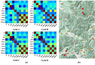
Figure 1: (a) Pearson Correlation Matrices of Different Weather Factors. Warm colors indicate a strong correlation, while cool colors indicate a weak correlation. (b) Locations and Terrains of the Four Grids. Grids A, C and D are on the uphill, while B is in a valley.

Firstly, different weather factors interact in complicated ways, while the interactions vary regionally. Although physics could interpret partially, much more highly complex and nonlinear dependencies among different weather factors still remain untractable from the data-driven perspective. For instance, air temperature, humidity, and rainfall are highly interdependent, as an increase in air temperature leads to a rise in atmospheric humidity, facilitating cloud formation and precipitation (Moran and Moran 2009). Similarly, air pressure, wind speed, and wind direction also display intricate interrelationships. In addition, some external factors, especially topography, exert a significant influence on meteorological conditions (Moran and Moran 2009). Mountains, plateaus, and canyons affect wind direction and speed, leading to unique climate phenomena, e.g., canyon wind and valley wind. Terrain also influences temperature distribution via its effect on solar radiation, with height, slope, and orientation playing critical roles. Fig. 1 illustrates how weather factors correlate in different grids, where each grid represents a specific region. Grids A and B exhibit different correlation patterns due to different terrains (A is located uphill, whereas B sits in a valley. )

Secondly, spatial dependencies among different regions/grids are complicated due to varied terrain and atmospheric motions. The weather conditions in one region can significantly impact other regions, leading to potential spatial dependencies. For example, the spatial distribution and intensity of rainfall can affect the rainfall in surrounding areas. In addition, as depicted in Fig. 2, the similarity of 100m wind speed between different grids is highly coincidental with the similarity of terrain, where wind speed patterns on land and ocean are contrasting. Therefore, investigating the spatial dependencies of different regions is crucial for effectively correcting NWP biases.

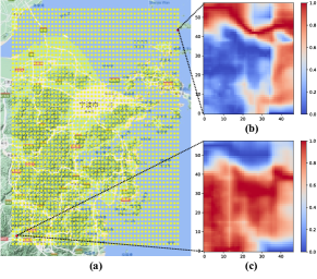
Figure 2: (a) Grid Distribution and Terrain of the Ningbo Dataset. (b) and (c) DTW similarity of 100m wind speed at one oceanic grid and one land grid with other grids.

To this end, we propose WeatherGNN, a GNN-based model that leverages meteorologic and geographic relationships efficiently for local NWP bias-correction. WeatherGNN mainly consists of a factor-wise GNN that employs factor and geographic embeddings to learn intra-grid meteorological interactions considering terrain heterogeneity, and a fast hierarchical GNN that adopts a pre-defined hierarchical structure and a dynamic adjustment to learn inter-grid spatial dependencies according to domain knowledge and weather dynamics. The main contributions are summarized as:

• We propose WeatherGNN that considers meteorologic and geographic relationships via GNNs for local NWP bias-correction in a unified framework. To the best of our knowledge, none of the preceding works have incorporated GNNs and domain knowledge simultaneously for this task.

• We introduce a factor-wise GNN to model terrain-specific meteorologic interactions adaptively and a fast hierarchical GNN to capture hierarchical spatial relationships dynamically. By leveraging domain knowledge, fast hierarchical message passing can achieve a linear complexity with respect to the number of grids, enhancing the efficiency and scalability of WeatherGNN.

• Extensive experimental results on two real-world datasets demonstrate the superiority of WeatherGNN, with an average improvement of 40.50% on RMSE compared to the original NWP.

Related Work

Bias-correction for NWP. Bias-correction methods have evolved from classical statistical methods, e.g., correcting the variance and average (Zhang et al. 2019), to shallow machine learning methods, e.g., deep belief networks (Hu et al. 2021) and SVM (Yoshikane and Yoshimura 2022). At present, a majority of DL works have emerged and achieved advantageous correcting effects due to their strong representative abilities. They mainly rely on LSTM (Li et al. 2022; Yang et al. 2022), CNN (Han et al. 2021), or their hybrid models (Han et al. 2022) to correct certain common weather factors, e.g., wind speed and precipitation. Some advanced models have also been applied to NWP bias-correction tasks and have undergone impressive improvement. For example, a recent work (Ge et al. 2022) uses AFNO (Guibas et al. 2021a) to learn continuous status of the atmosphere from sparse and non-uniform weather observational data for grid-free bias-correction. However, these studies rarely consider meteorologic and geographic relationships within NWP comprehensively. Therefore, how to fully use such relationships to correct the bias within NWP is still an open problem.

DL methods for spatial-temporal modeling. DL methods for spatial-temporal modeling have shown promising results in various applications, e.g., video action recognition (Cai, Yao, and Chen 2021), time series analysis (Chen, Gel, and Poor 2022; Liu et al. 2022), and earth system modeling (Gao et al. 2022). These methods can capture relationships between spatial and temporal dimensions and help to understand the underlying structure and dynamics of the spatial-temporal data. Some of them have been widely used due to their good generalization and model capacity, e.g., 3D convolutions (Guo et al. 2019; Luo and Yuille 2019), attention (Yan et al. 2019; Karim et al. 2022; Wei et al. 2022), Vison Transformers (ViT) (Dosovitskiy et al. 2020), and spatial-temporal graph neural networks (STGNNs) (Cai et al. 2019; Vazquez-Enriquez et al. 2021). In particular, STGNNs demonstrate superior performance when dealing with complex spatial-temporal data. They combine the strengths of GNNs with RNNs, CNNs, or attentions to capture dynamic changes in spatial dependencies over time (Yu, Yin, and Zhu 2018; Bai et al. 2020; Wu et al. 2020; Chen et al. 2020). However, STGNNs face the challenges of designing graph structures in particular scenarios and performing efficient message passing across the graph, especially on large-scale datasets.

DL methods for medium-range global weather forecasting. Since 2022, DL weather models have made significant progress in medium-range global weather forecasting (Rasp et al. 2023). For example, FourCastNet (Pathak et al. 2022) generates global forecasts based on AFNO. Pangu (Bi et al. 2023), Fengwu (Chen et al. 2023a), Fuxi (Chen et al. 2023b), and ClimaX (Nguyen et al. 2023) extend hierarchical ViT architectures by plug-and-play modules, e.g., model-specific encoder-decoders and buffer mechanisms, to make longer global forecasts. GraphCast (Lam et al. 2022) follows a GNN architecture and designs a multi-scale unweighted mesh graph to make autoregressive global forecasts. However, due to computational constraints, these global models do not consider the complex relationships between weather factors and terrain as WeatherGNN does. Thus, they fail to capture the detailed local weather patterns characterized by the complex interactions between different weather factors and the corresponding terrain. This leads to a gap between global weather forecasting and local weather forecasting, which highlights the need for bias-correction models in local NWP.

WeatherGNN

We formalize the problem of local NWP bias-correction and describe how to model both intra-grid meteorologic interactions and inter-grid spatial dependencies using WeatherGNN.

Problem Definition

The goal of local NWP bias-correction is to reduce the difference between origin NWP and observations for a specific region. The NWP data are represented as a sequence $\left[\mathcal{X}_{i}\right]_{i=1}^{T}$, and $\left[\mathcal{X}_{i}\right]_{i=1}^{T}\in\mathbb{R}^{N\times F_{\text{e}}\times T}$, where $N$ denotes the number of grids in this region , $F_{\text{e}}$ denotes the number of weather factors (e.g., temperature, humidity, and wind speed), and $T$ is the length of sequence. Similarly, $\left[\mathcal{Y}_{i}\right]_{i=1}^{T}\in\mathbb{R}^{N\times F_{\text{e}}\times T}$ represents the corresponding weather observations. Moreover, each grid has associated geographic information denoted as $\mathcal{Z}\in\mathbb{R}^{N\times F_{\text{g}}}$, where $F_{\text{g}}$ is the dimension of geographic features (e.g., longitude, latitude, and altitude). The local NWP bias-correction problem aims to learn a function $f(\cdot)$ that maps weather forecasts to observations incorporating the geographic features:

$$\{[\mathcal{X}_{i}]_{i\in\Omega(t)};\mathcal{Z}\}\xrightarrow{f(\cdot)}\mathcal{Y}_{t},$$ (1)

$$\Omega(t)=\{t-\tau,\cdots,t-1,t,t+1,\cdots,t+\tau\},$$

where $\Omega(t)$ denotes a temporal window around time step $t$ with length $T=2\tau+1$ , as we consider a period of time before and after $t$ when correcting $\mathcal{X}_{t}$. For simplicity, in the remainder of the paper, we denote $\left[\mathcal{X}_{i}\right]_{i\in\Omega(t)}$ and $\mathcal{Y}_{t}$ by $\boldsymbol{X}$ and $\boldsymbol{Y}$, respectively.

Model Overview

As illustrated in Fig. 3, WeatherGNN follows a two-branch architecture. The NWP sequences associated with the geographic features are input into factor-wise GNN and fast hierarchical GNN to capture the intra-grid meteorologic interactions and inter-grid spatial dependencies, respectively, and then mapped to corrected results.

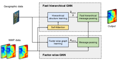
Figure 3: An Overview of WeatherGNN.

Learning Meteorologic Interactions via Factor-Wise Graph Neural Networks

As previously discussed, accurately capturing the meteorologic interactions in different terrains is crucial for effectively correcting NWP biases. However, manually defining the correlations between different factors for each grid is challenging due to the significant time cost involved, as well as issues with applicability. To address this problem, we propose a factor-wise graph learning (FGL) module that allows for automatic exploration of the hidden interrelationships between weather factors for each grid, while also considering variations in the terrain.

Factor-wise graph learning. The FGL module first randomly initializes a learnable factor embedding dictionary $\boldsymbol{E}_{\text{f}}\in\mathbb{R}^{F_{\text{e}}\times d}$ for all weather factors, where each row corresponds to the embedding vector for each factor, and $d$ is the dimension of factor embedding. This embedding is jointly optimized through model training to learn the hidden dependencies among different factors. Then, we take the geographic information of each grid $\mathcal{Z}$ as input and encode it with an MLP to obtain the grid-specific geographic embedding matrix $\boldsymbol{E}_{\text{g}}=\mathrm{MLP}(\mathcal{Z})\in\mathbb{R}^{N\times d}$ of all grids, where $N$ is the number of grids. Given the factor embedding and grid-specific geographic embedding, we can infer relationships between weather factors for each grid by first computing grid-specific factor embedding $\boldsymbol{E}$ and then multiplying $\boldsymbol{E}$ and $\boldsymbol{E}^{\top}$:

$$\boldsymbol{E}_{i}=\boldsymbol{E}_{\text{f}}+\boldsymbol{E}_{\text{g},i},$$ (2)

$$\boldsymbol{A}_{\text{intra},i}=\mathrm{Softmax}(\boldsymbol{E}_{i}\boldsymbol{E}_{i}^{\top}),$$

$$\boldsymbol{A}_{\text{intra}}=\{\boldsymbol{A}_{\text{intra},i}\}_{i=1}^{N},$$

where $\boldsymbol{E}_{i}\in\mathbb{R}^{F_{\text{e}}\times d}$ is the grid-specific factor embedding of grid $i$ considering geographic information. $\boldsymbol{A}_{\text{intra},i}\in\mathbb{R}^{F_{\text{e}}\times F_{\text{e}}}$ represents the adjacency matrix of intra-grid factor-wise graph of grid $i$. FGL module can efficiently discover meteorologic interactions for each grid and has interpretability.

Factor-wise GNN. Finally, enhanced by FGL, factor-wise GNN can be formulated as:

$$\boldsymbol{H}_{i}=\mathrm{GNN}(\boldsymbol{X}_{i},\boldsymbol{A}_{\text{intra},i}),$$ (3)

where $\boldsymbol{X}_{i}\in\mathbb{R}^{F_{\text{e}}\times T}$ is the NWP data of grid $i$, and $\boldsymbol{H}_{i}\in\mathbb{R}^{F_{\text{e}}\times d}$ is the corresponding output hidden state considering meteorologic interactions. $\mathrm{GNN}(\cdot)$ can be different variants of Graph Neural Networks, and we choose GCN (Kipf and Welling 2016) for simplicity. This factor-wise message passing is performed for each grid in parallel, obtaining the final output $\boldsymbol{H}=\{\boldsymbol{H}_{i}\}_{i=1}^{N}\in\mathbb{R}^{N\times F_{\text{e}}\times d}$. Moreover, according to Lemma 1, the factor-wise GNN has an $O(N)$ complexity.

Learning Spatial Dependencies via Fast Hierarchical Graph Neural Networks

Another crucial aspect of accurate bias-correction is incorporating the complicated spatial dependencies that exist between different grids. However, due to the intricate nature of terrains and varying weather conditions, achieving this is a nontrivial task. To address this challenge, we propose the fast hierarchical GNN (FHGNN) that can effectively capture the inter-grid spatial dependencies. FHGNN involves several steps. First, we compute the initial spatial proximity of grids based on meteorologic and geometric distance and then construct the hierarchical structure by iteratively clustering grids into multi-level clusters (i.e., super-grids), where grids from the same cluster in lower levels are more relevant and should interact with each other. Next, we adjust the spatial proximity with the attention matrix based on the current weather conditions. Finally, a fast hierarchical message passing (FHMP) module is introduced to model the inter-grid spatial dependencies, which conducts fine-grained interactions among grids at low level but coarse-grained interactions at high level. Furthermore, FHGNN is able to achieve a linear complexity w.r.t. the number of grids, while vanilla GNN has a square complexity.

Constructing hierarchical structure based on domain knowledge. We construct the hierarchical structure of grids based on pre-defined heuristic rules considering meteorologic and geographic distance. We calculate meteorologic distance matrix $\boldsymbol{W}$ by computing dynamic time warping (DTW) (Müller 2007) distance between weather sequences of each grid and the 3D geographic distance matrix $\boldsymbol{D}$ based on the latitude, longitude, and altitude information of grids obtained from geographic features $\mathcal{Z}$. Specifically, the two distance matrices are calculated as follows:

$$\boldsymbol{W}_{ij}^{f}=\mathrm{DTW}(\boldsymbol{\mathsf{X}}_{i}^{f},\boldsymbol{\mathsf{X}}_{j}^{f}),\boldsymbol{W}_{ij}=\frac{1}{F_{\text{e}}}\Sigma_{f=1}^{F_{\text{e}}}\boldsymbol{W}_{ij}^{f},$$ (4)

$$\boldsymbol{D}_{ij}=\sqrt{\lambda_{\text{lat}}d_{\text{lat},ij}^{2}+\lambda_{\text{lon}}d_{\text{lon},ij}^{2}+\lambda_{\text{alt}}d_{\text{alt},ij}^{2}},$$ (5)

where $\boldsymbol{\mathsf{X}}_{i}^{f}$ and $\boldsymbol{\mathsf{X}}_{j}^{f}$ are the time series of the $f$-th weather factor of grid $i$ and $j$ in the whole training data, respectively. $\boldsymbol{W}_{ij}^{f}$ is the $(i,j)$-th entry of $\boldsymbol{W}^{f}$, which is the DTW distance matrix of all gird-pairs w.r.t weather factor $f$. $\boldsymbol{W}$ represents the average of DTW distance matrix of all weather factors. $d_{\text{lat},ij}$, $d_{\text{lon},ij}$, $d_{\text{alt},ij}$, are the latitude, longitude, and altitude distance between grid $i$ and $j$, respectively, with $\lambda_{(\cdot)}$ being the corresponding coefficients to adjust the importance of these distances for calculating the geographic distance. Then, Gaussian kernels are applied to compute the corresponding similarity matrices, i.e., $\boldsymbol{A}_{\text{met}}$ and $\boldsymbol{A}_{\text{geo}}$, which are further combined to represent the inter-grid spatial proximity matrix. The process is formulated as:

$${\boldsymbol{A}}_{\text{met}}=\text{exp}(-\boldsymbol{W}^{2}/\sigma_{\text{met}}^{2}),\quad{\boldsymbol{A}}_{\text{geo}}=\text{exp}(-\boldsymbol{D}^{2}/\sigma_{\text{geo}}^{2}),$$ (6)

$$\boldsymbol{A}_{\text{inter}}={\boldsymbol{A}}_{\text{met}}+{\boldsymbol{A}}_{\text{geo}},$$

where $\sigma_{(\cdot)}$ are hyperparameters to control the scale of the corresponding Gaussian kernels, which ensures both matrices have a similar range of values.

Afterward, we adopt a clustering algorithm, e.g., K-means, to cluster grids into multi-level super-grids based on $\boldsymbol{A}_{\text{inter}}$ to construct the hierarchical structure. The clustering procedure is performed for $L$ iterations, and at the $l$-th iteration, we cluster the grids at level $l$ into the next coarsened super-grids at level $l+1$. We denote the assignment matrix returned from the clustering algorithm at level $l$ as $\boldsymbol{S}^{l}\in\{0,1\}^{N^{l}\times N^{l+1}}$, where each row contains one 1, and others are 0s representing the assignment of each grid at level $l$ to a super-grid at level $l+1$. $N^{l}$ is the number of grids at level $l$. Besides, we compute the spatial proximity matrix $\boldsymbol{A}^{l}$ for each level. The construction procedure of the hierarchical structure can be formulated as:

$$\boldsymbol{S}^{l}\leftarrow\text{K-means}(\boldsymbol{A}^{l}),$$ (7)

$$\boldsymbol{A}^{l}=(\boldsymbol{S}^{l-1})^{\top}\boldsymbol{A}^{l-1}\boldsymbol{S}^{l-1},\quad\boldsymbol{A}^{0}=\boldsymbol{A}_{\text{inter}},$$

where, $\boldsymbol{A}^{l}\in\mathbb{R}^{N^{l}\times N^{l}}$ ($l=1,2,\cdots,L$) is the spatial proximity matrix at level $l$, which takes $\boldsymbol{A}^{l-1}$ and generates a coarsened proximity matrix denoting the connectivity strength between super-grids at level $l$.

Moreover, we generate mask matrix $\boldsymbol{M}^{l}$ to make the spatial proximity matrices sparse, where the $(i,j)$-th entry $\boldsymbol{M}^{l}_{ij}=1$ if grids $i$ and $j$ belong to the same cluster, and $\boldsymbol{M}^{l}_{ij}=0$ otherwise, as grids belonging to the same cluster have stronger interrelationships that are preferred to reserve.

Dynamic adjustment of spatial dependencies based on NWP data. Spatial dependencies are also dependent on the weather conditions. For example, in windy weather, a grid has a strong correlation with its upwind grids. Thus, we encode the input NWP data $\boldsymbol{X}$ and utilize the attention matrix to adaptively adjust the spatial proximity matrices. This dynamic adjustment is formulated as :

$$\begin{split}&\boldsymbol{H}^{0}_{\text{Q}}=\boldsymbol{X}\boldsymbol{W}_{\text{Q}},\quad\boldsymbol{H}^{0}_{\text{K}}=\boldsymbol{X}\boldsymbol{W}_{\text{K}},\\ &\boldsymbol{H}^{l}_{\text{Q}}=(\boldsymbol{S}^{l-1})^{\top}\boldsymbol{H}^{l-1}_{\text{Q}},\quad\boldsymbol{H}^{l}_{\text{K}}=(\boldsymbol{S}^{l-1})^{\top}\boldsymbol{H}^{l-1}_{\text{K}},\\ \end{split}$$ (8)

$$\tilde{\boldsymbol{A}}^{l}=\boldsymbol{M}^{l}\odot\mathrm{Softmax}(\boldsymbol{H}_{\text{Q}}^{l}{\boldsymbol{H}_{\text{K}}^{l}}^{\top}/\sqrt{d}\odot\boldsymbol{A}^{l}).$$ (9)

In Equation 8, $\boldsymbol{H}^{0}_{\text{Q}},\boldsymbol{H}^{0}_{\text{K}}\in\mathbb{R}^{N\times d}$ are calculated by linear projections of input NWP data $\boldsymbol{X}\in\mathbb{R}^{N\times F_{\text{e}}\times T}$ with parameters $\boldsymbol{W}_{\text{Q}},\boldsymbol{W}_{\text{K}}\in\mathbb{R}^{F_{\text{e}}\times T\times d}$, respectively. These representations are iteratively aggregated according to the cluster assignment matrix, generating representations $\boldsymbol{H}^{l}_{\text{Q}},\boldsymbol{H}^{l}_{\text{K}}\in\mathbb{R}^{N^{l}\times d}$ for super-grids at each level. In Equation 9, $\odot$ denotes element-wise product and the spatial proximity matrix is adjusted with the attention matrix. Moreover, the mask $\boldsymbol{M}^{l}$ is used to make the spatial proximity matrix sparse, where only interactions of grids belonging to a same cluster are reserved.

Fast hierarchical message passing. Hierarchical message passing (FHMP) module enables the model to capture the hierarchical inter-grid spatial dependencies. The main idea of FHMP is conducting fine-grained message passing among low-level grids but coarse-grained interactions at high level to simplify and distill the redundant spatial dependencies as well as accelerate the computation. Formally, FHMP module can be formulated as:

$$\begin{split}\text{Message}&:\hat{\boldsymbol{H}}^{l}=\boldsymbol{H}^{l}\boldsymbol{W}^{l},\boldsymbol{H}^{l}=(\boldsymbol{S}^{l-1})^{\top}\boldsymbol{H}^{l-1},\\ \text{Aggregation}&:\tilde{\boldsymbol{H}}^{l}_{v^{l}}=\frac{1}{|\mathcal{N}_{v^{l}}|}\sum_{u^{l}}\tilde{\boldsymbol{A}}_{u^{l}v^{l}}^{l}\hat{\boldsymbol{H}}^{l}_{u^{l}},\\ &\forall v^{l}\in[0,1,2,\cdots N^{l}-1],\mathcal{N}_{v^{l}}=\{u^{l}|\tilde{A}^{l}_{u^{l}v^{l}}\neq 0\},\\ \text{Duplication}&:\boldsymbol{H}^{\prime}=\tilde{\boldsymbol{H}}^{0}+\sum_{l=1}^{L}\prod_{i=0}^{l-1}\boldsymbol{S}^{i}\tilde{\boldsymbol{H}}^{l},\\ \text{Update}&:\boldsymbol{H}^{\prime\prime}=\boldsymbol{H}+\boldsymbol{H}^{\prime}\boldsymbol{W},\end{split}$$ (10)

where $\hat{\boldsymbol{H}}^{l}\in\mathbb{R}^{N^{l}\times d}$ are calculated by linear projections of $\boldsymbol{H}^{l}$, representing the message of grids at level $l$, and $\boldsymbol{H}^{0}=\boldsymbol{H}$ is the output of the factor-wise GNN (see Equation 3). For a specific grid $v_{l}$ at level $l$, its neighbors $\mathcal{N}_{v^{l}}$ are identified by the spatial proximity matrix $\tilde{\boldsymbol{A}}^{l}$. $v_{l}$ then aggregates its neighbors’ messages according to the proximity strength in $\tilde{\boldsymbol{A}}^{l}$. The duplication stage is the key design of FHMP module . It duplicates the messages from the super-grids at each level to their containing grids at level 0 based on assignment matrices $[S^{i}]^{L-1}_{i=0}$, and the grids at level 0 belonging to the same super-grid share the same message from $\hat{\boldsymbol{H}}^{l}$, as illustrated in Fig. 4. With appropriate hierarchical structure, all grid-pairs at level 0 can interact. After collecting the messages from all levels, the hidden representations of grids at level 0 are updated based on integrated messages with a residual connection. According to Lemma 1, both dynamic adjustment and FHMP in FHGNN have a linear complexity w.r.t. the number of grids. The proof is in Appendix A.

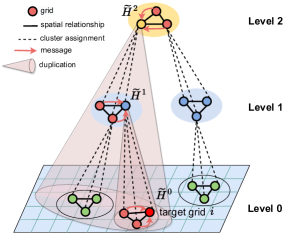
Figure 4: An Overview of Fast Hierarchical Message Passing.

Lemma 1.

The complexity of factor-wise GNN and fast hierarchical GNN is $O(N)$, where $N$ is the number of grids.

Bias-Correction Output

Given the output $\boldsymbol{H}^{\prime\prime}\in\mathbb{R}^{N\times d}$ of FHGNN, we feed it into an MLP-based decoder to produce corrected weather factors for each grid at the target time step at once. We adopt the L1 loss function to compare the difference between corrected results and ground truth, which can be formulated as: $\mathcal{L}(\hat{\boldsymbol{Y}},\boldsymbol{Y})=\sum_{f=1}^{F_{\text{e}}}w_{f}\|\hat{\boldsymbol{Y}}^{f}-\boldsymbol{Y}^{f}\|_{1}$, where $\hat{\boldsymbol{Y}}=\mathrm{MLP}\left(\boldsymbol{H}^{\prime\prime}\right)$, and $\hat{\boldsymbol{Y}}^{f}$ and $\boldsymbol{Y}^{f}$ are the corrected results and the ground truth of the weather factor $f$, and $w_{f}$ is a hyperparameter representing the corresponding weights.

Experiments

Datasets

We collect two real-world bias-correction datasets: Ningbo and Ningxia, covering two different terrain types in China. Each grid in both datasets has three types of data, i.e., geographic data, NWP data, and observational weather data. In addition, geographic data contain latitude, longitude, and DEM (commonly used in geographic information systems to represent terrain) information. Ningbo dataset depicts a coastline area with latitude range $28.85^{\circ}$N$-30.56^{\circ}$N and longitude range $120.91^{\circ}$E$-122.29^{\circ}$E. There are 58$\times$47 grids with a grid size of 0.03 degree in latitude and longitude. Both NWP and observational weather data have hourly records including 10 weather factors from 1/Jan/2021 to 1/Apr/2021. Ningxia dataset features mountainous and hilly terrain with latitude range $34.5^{\circ}$N$-42^{\circ}$N and longitude range $106^{\circ}$E$-116^{\circ}$E. There are 31$\times$41 grids with grid size of 0.25 degree in latitude and longitude. Both NWP and observational weather data have hourly records including 8 weather factors from 1/Jan/2021 to 1/Jan/2022. In our experiments, we divide each dataset into training/validation/test subsets using a 7:1:2 ratio in chronological order. We define a temporal window of 7 time steps for NWP bias-correction, including the target time step, as well as the previous and next three steps. More dataset details are in Appendix B.

Table 1: Bias-correction performance comparison of each weather factor on the Ningbo and Ningxia datasets. Bold and Underline indicate the best and second best performance, respectively. $\Delta$ denotes the relative improvement between WeatherGNN and best baselines/NWP. $*$ indicates the backbone models of global weather forecasting models.

Factor	Metric	NWP	BiLSTM-T	HybridCBA	ConvLSTM	AFNO∗	Swin∗	STGCN	HGCN∗	MegaCRN	WeatherGNN	$\Delta$ Baseline	$\Delta$ NWP
Ningbo
100ws	MAE	2.26	1.98	1.53	1.37	0.84	0.91	0.94	0.89	0.87	0.81	3.57%	64.16%
	RMSE	2.74	2.70	2.34	2.03	1.17	1.26	1.31	1.25	1.21	1.15	1.71%	58.03%
10ws	MAE	1.38	1.37	1.18	0.91	0.58	0.67	0.65	0.63	0.61	0.56	3.45%	54.35%
	RMSE	1.71	1.69	1.65	1.28	0.81	0.87	0.91	0.88	0.85	0.79	2.47%	49.12%
h	MAE	15.37	14.48	12.32	7.61	5.86	5.96	6.35	5.81	5.95	5.65	2.75%	63.24%
	RMSE	18.28	18.44	15.29	10.35	7.26	7.32	8.29	7.28	7.80	7.13	1.79%	61.00%
2t	MAE	1.28	1.20	1.19	1.16	0.93	1.10	1.12	1.04	0.91	0.91	0.00%	28.91%
	RMSE	1.74	1.54	1.58	1.51	1.27	1.34	1.47	1.31	1.23	1.26	-2.44%	27.59%
tp	MAE	0.143	0.412	0.331	0.309	0.123	0.240	0.282	0.212	0.131	0.116	5.69%	18.88%
	RMSE	0.495	0.811	0.763	0.655	0.391	0.587	0.627	0.502	0.435	0.342	12.53%	30.91%
Ningxia
100ws(U)	MAE	2.93	2.69	2.33	2.22	2.00	2.12	2.33	2.08	1.95	1.79	8.21%	38.91%
	RMSE	3.83	3.41	2.99	2.87	2.58	2.81	3.01	2.69	2.54	2.41	6.59%	37.08%
100ws(V)	MAE	3.39	2.79	2.67	2.51	2.25	2.30	2.51	2.29	2.27	2.14	4.89%	36.87%
	RMSE	4.52	3.59	3.43	3.24	2.93	3.11	3.22	3.03	2.94	2.69	8.19%	40.49%
10ws(U)	MAE	1.79	1.65	1.44	1.40	1.22	1.22	1.52	1.33	1.23	1.18	3.28%	34.08%
	RMSE	2.38	2.16	1.87	1.84	1.60	1.64	1.97	1.73	1.60	1.53	4.38%	35.71%
10ws(V)	MAE	2.03	1.73	1.55	1.50	1.32	1.41	1.56	1.38	1.35	1.22	7.58%	39.90%
	RMSE	2.74	2.24	2.02	1.96	1.75	2.08	2.01	1.85	1.80	1.61	8.00%	41.24%
2t	MAE	2.81	2.71	2.72	2.44	2.27	2.27	2.54	2.20	2.28	2.23	-1.36%	20.64%
	RMSE	3.74	3.49	3.54	3.15	2.91	2.89	3.27	2.79	2.92	2.85	-2.15%	23.80%

Table 2: Ablation study on the 100m wind speed of the Ningbo and Ningxia datasets.

Factor		Ningbo 100ws		Ningxia 100ws(U)
Metric		MAE	RMSE	MAE	RMSE
Variant	shared-F	0.84	1.19	1.87	2.49
	no-F	0.92	1.27	1.95	2.57
	geo-H	0.91	1.26	2.04	2.61
	met-H	0.89	1.26	1.93	2.58
	static-H	0.86	1.23	1.90	2.52
	no-H	0.96	1.32	2.35	2.83
WeatherGNN		0.81	1.15	1.79	2.41

Baselines and Experimental Settings

We compare WeatherGNN with state-of-the-art models, including: BiLSTM-T (Yang et al. 2022): using BiLSTM considering multiple covariates for bias-correction; HybridCBA (Han et al. 2022): combining CNN, BiLSTM, and attention mechanism to deal with relationships between target factor and other factors; ConvLSTM (Shi et al. 2015): extending LSTM with convolutional gates; AFNO (Guibas et al. 2021b): adopting Fourier neural operator to capture features adaptively. Since FourCastNet (Pathak et al. 2022) is purely on AFNO, we regard AFNO as the backbone model of FourCastNet; Swin (Liu et al. 2021): constructing a hierarchical transformer by a shifted windowing scheme. Since Pangu (Bi et al. 2023) is the variation of Swin with two additional strategies, i.e., a 3D transformer encoder to formulate data and a hierarchical aggregation algorithm to alleviate errors, we treat Swin as the backbone model of Pangu; HGCN (Guo et al. 2021): operating hierarchical GNNs to utilize hierarchical spatial dependencies. Since GraphCast (Lam et al. 2022) adopts static hierarchical graphs, we treat HGCN as the backbone model of GraphCast. STGCN (Yu, Yin, and Zhu 2018): deploying graph convolution and temporal convolution to capture spatial and temporal relationships; MegaCRN (Jiang et al. 2023): introducing adaptive graphs to learn underlying heterogeneous spatial dependencies. Notably, for our local NWP bias-correction task, we compare the performance of backbone models, i.e., AFNO, Swin, and HGCN, as that of global weather models.

Baselines and WeatherGNN are implemented with Pytorch, executed on a server with one 32GB Tesla V100 GPU card, and well-tuned according to the performance on the validation set. The hyperparameter settings are summarized in Appendix C. We optimize all models using Adam optimizer with an initial learning rate of 0.003 and set the maximum number of epochs to 100. We halt training when the validation loss does not decrease for 15 consecutive epochs.

Performance Comparison

We use Mean Absolute Error (MAE) and Root Mean Square Error (RMSE) to measure the performance of all models. As shown in Table 1, the results lead to the following findings: (1) NWP can be significantly corrected, and our proposed WeatherGNN has an average improvement of over 40% in correcting weather factors compared with the original NWP. (2) Although baselines, especially AFNO and MegaCRN, have shown competitive performance, WeatherGNN achieves the best performance in 17 out of 20 cases across two datasets, despite the slight inferiority in 2m temperature correction. One possible reason is that the 2m temperature factor varies slowly in time and space, and thus considering complicated meteorologic and geographic relationships for correcting this measure may not be necessary. (3) The bias-correction of WeatherGNN on wind speed is significant. Given the fact that the mechanism of wind formation is complex and wind speed changes over time and space rapidly, it is possible that the dynamic adjustment in fast hierarchical GNN helps WeatherGNN adapt to weather dynamics.

Model Analysis

Figure 5: Model Efficiency Comparison.

Figure 6: Visualization of Bias-Correction on Ningbo Dataset. Each row corresponds to a meteorologic factor and each column corresponds to an algorithm.

Ablation study. To evaluate the effectiveness of factor-wise GNN and fast hierarchical GNN of WeatherGNN, we conduct ablation studies on correcting the 100m wind speed of two datasets. For factor-wise GNN, we design variants: (1) shared-F: only using the factor embedding to construct a shared factor graph for all grids, ignoring spatial heterogeneity; (2) no-F: replacing the factor graphs with a one-layer MLP to encode the weather information without considering the meteorological interactions explicitly. For fast hierarchical GNN, we design variants: (3) geo-H: constructing the hierarchy only using geographic distances; (4) met-H: constructing the hierarchy only using DTW similarity of weather factor time series; (5) static-H: removing the dynamic adjustment and only adopting the static hierarchy when performing fast hierarchical message passing; (6) no-H: only using the $\boldsymbol{A}_{\text{inter}}$ calculated by Eq. 6 to model spatial dependencies between grids without constructing the hierarchy.

All designs in WeatherGNN are proven to be effective based on the results in Table 2. Besides, we have other findings: (1) Terrain is crucial for bias-correction, even when it is solely used as input (as shown in "no-F"). By comparing "shared-F" and "no-F", we observe that modeling the relationships between factors explicitly can further improve the correction outcomes. Notably, making such relationships adapt to the changing terrain can enhance the correction effect. This discovery validates the effectiveness of our factor-wise GNN. (2) Constructing a hierarchical structure with geographic and meteorologic distances significantly improves the bias-correction performance. The meteorologic distance is found to be more effective than geographic distance, possibly because the influence of geography on weather factors is partly reflected in the weather factor sequences and DTW similarity can help to discover underlying spatial dependencies. Besides, the meteorologic distance is helpful to unveil remote inter-grid dependencies. Furthermore, the hierarchical design integrating both factors achieves the best results.

Model efficiency. We evaluate the efficiency of WeatherGNN and baselines by increasing the number of grids and measuring running time and GPU memory usage. Fig. 5 illustrates that WeatherGNN (linear complexity) performs faster and requires less GPU memory than baselines. More results are in Appendix D. The efficiency advantages of WeatherGNN indicate good scalability, showing strong potential for application in large regions (e.g., continental or global applications).

Case study. We conduct case studies of bias-correction effects of different models and the learned factor-wise graph of WeatherGNN. Also, studies of prior hierarchical structures based on meteorologic and geometric distance and dynamic adjustment of spatial dependencies are in Appendix E. The cases of extreme weather, i.e., blustery weather, are in Appendix F.

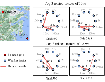
Figure 7: The Illustration of Learned Factor-Wise Graphs of Two Grids on Two Different Types of Terrains.

Bias-correction effects: We conduct a case study to investigate the bias-correction effects. We visualize the observation data at 22:00 6/Apr/2021 with origin NWP as well as corrected outputs of AFNO, MegaCRN, and WeatherGNN on measures of 2m temperature(2t), humidity(h), 10m wind speed(10ws), and 100m wind speed(100ws). As shown in Fig. 6, NWP has a large deviation from the ground truth, while baselines and WeatherGNN can effectively reduce this discrepancy. In particular, due to the comprehensive consideration of the relationships among factors and among grids, WeatherGNN demonstrates stable and excellent bias-correction effects.

Factor-wise graphs: Fig. 7 shows an example of the learned factor-wise graphs selected randomly. Grid 500 locates in the mountains and Grid 2555 is in the ocean. 10ws and 100ws at both grids are closely related to each other. However, 10ws of Grid 500 is more relevant to pressure, as the mountainous regions have diverse terrain and are prone to rapid changes in air pressure, resulting in great effects on wind speeds. On the other hand, 10ws of Grid 2555 is affected by 10div (10m horizontal divergence, a measure of the local spreading or divergence of wind field in a horizontal plane at the height of 10 meters). One of the possible reasons is that on the sea horizon, the expansion of air in the horizontal direction has a significant impact on wind speed.

Conclusion and Future Work

In this paper, we propose WeatherGNN, a GNN-based model that leverages meteorologic and geographic relationships efficiently for local NWP bias correction. Specifically, we introduce a factor-wise GNN and a fast hierarchical GNN to capture intra-grid and inter-grid dependencies in weather factors, achieving linear complexity with respect to the number of grids. Extensive experimental results demonstrate the superiority of WeatherGNN. In the future, we will investigate the use of WeatherGNN for other meteorological applications, e.g., weather forecasting and downsampling. We also plan to apply WeatherGNN to larger real-world regions to investigate its scalability and robustness across different climatic and geographical conditions.

WeatherGNN: Exploiting Complicated Relationships in Numerical Weather

Prediction Bias Correction (Appendix)

Appendix A A. Model Complexity Analysis

Lemma 1. The complexity of the factor-wise GNN and fast hierarchical GNN is $O(N)$, where $N$ is the number of grids.

Proof.

First, as the factor-wise GNN performs graph learning and message passing within each grid, it is straightforward to derive that the complexity is $O(N(F_{\text{e}})^{2}d)=O(N)$, where the number of weather factors $F_{\text{e}}$ and the hidden dimension $d$ are constant.

To analyze the complexity of the fast hierarchical GNN, we introduce additional notations. Besides the number of grids $N$, the number of levels $L$, and the number of super grids at level $l$ $N^{l}$, we introduce $k$ to represent the cluster size (i.e., the number of grids belonging to a cluster), which can be set in different clustering algorithms. Note that the cluster size $k$ and the dimension of hidden representations $d$ are constants. We can derive that $N^{l+1}=\frac{N^{l}}{k}$ and $L=\mathrm{log}_{k}N$.

The number of entries in spatial proximity matrix $\tilde{\boldsymbol{A}}^{l}$ in all $L$ levels reserved by mask matrix $\boldsymbol{M}^{l}$ is $k^{2}\sum_{l=1}^{L}N^{l}=k^{2}\sum_{l=1}^{L}\frac{N}{k^{l}}=\frac{k^{2}N}{k-1}$, and thus the complexity of dynamic adjustment is $O(N)$.

Moreover, according to Eq. 10, the complexity of FHMP can be divided into four stages:

Message: The complexity of obtaining the messages $\hat{\boldsymbol{H}}^{l}$ at level $l$ is $O(N^{l})$. For all levels, the summed complexity is $\sum_{l=0}^{L}N^{l}=\sum_{l=0}^{L}\frac{N}{k^{l}}$. It is easy to verify that $O(\sum_{l=0}^{L}\frac{N}{k^{l}})=O(\frac{kN}{k-1})=O(N)$.

Aggregation: This stage aggregates the messages in the same cluster, resulting in $k^{2}$ messages for each cluster, and the number of clusters is $\sum_{l=1}^{L}N^{l}=\sum_{l=1}^{L}\frac{N}{k^{l}}$. Thus, the complexity of Aggregation is $O(k^{2}\sum_{l=1}^{L}\frac{N}{k^{l}})=O(\frac{k^{2}N}{k-1})=O(N)$.

Duplication: Since the hierarchical structure is pre-defined, the mapping between super grids at level $l>0$ and grids at level 0, i.e., $\prod_{i=0}^{l-1}S^{i}$, can be pre-calculated. Besides, $\prod_{i=0}^{l-1}S^{i}\tilde{\boldsymbol{H}}^{l}$ can be implemented with indexing operation with complexity $O(N^{l})$, as $\prod_{i=0}^{l-1}S^{i}$ only contains 0s and 1s. Therefore, the complexity of this stage is $O(\sum_{l=1}^{L}N^{l})=O(\frac{kN}{k-1})=O(N)$.

Update: The update stage involves an addition operation of complexity $O(N)$.

Therefore, the complexity of FHMP is $O(N)$. As for the impact of edges, in WeatherGNN, the number of edges is not constant but increases linearly with the number of nodes. This is because the nodes are clustered with the cluster size of a constant, and only the edges connecting nodes belonging to the same clusters are preserved. In general, the complexity of message passing in a GNN is $O(|V|+|E|)$ [1], where $|V|$ and $|E|$ are the numbers of nodes and edges, respectively. In our case, since the number of edges is linearly related to the number of nodes, the complexity of FHMP remains $O(N)$.

To this end, the overall complexity of all blocks in WeatherGNN is $O(N)$. ∎

[1] Hamilton, W. L. (2020). Graph representation learning. Morgan & Claypool Publishers.

Appendix B B. Dataset Description

Since the local NWP bias-correction task requires direct mapping between NWP and observational data, current public weather datasets cannot meet such requirements. We construct two real-world bias-correction datasets: Ningbo and Ningxia, covering two different terrain types in China. Each grid in both datasets has three types of data, i.e., geographic data, NWP data, and observational weather data. In addition, geographic data contain latitude, longitude, and DEM (commonly used in geographic information systems to represent terrain) information.

Ningbo: The Ningbo dataset depicts a coastline area with latitude ranges between $28.85^{\circ}$N to $30.56^{\circ}$N and longitude ranges between $120.91^{\circ}$E to $122.29^{\circ}$E. There are 58$\times$47 grids with a grid size of 0.03 degrees in latitude and longitude. The DEM data are collected from ETOPO1. The NWP and observational weather data are provided by Ningbo Meteorological Bureau. Both of them have hourly weather data including 10 weather factors from 1/Jan/2021 to 1/Apr/2021.

Ningxia: The Ningxia dataset features mountainous and hilly terrain with a latitude range of $34.5^{\circ}$N to $42^{\circ}$N and a longitude range $106^{\circ}$E to $116^{\circ}$E. There are 30$\times$40 grids with grid size of 0.25 degrees in latitude and longitude. The DEM data are collected from ETOPO1. The NWP is downloaded from commercial ECMWF’s forecasts . We treat the reanalysis weather data from ECMWF’s ERA5 as ground truth. Both NWP and ECMWF’s ERA5 data contain hourly weather data with 8 weather factors, ranging from 1/Jan/2021 to 1/Jan/2022.

The statistics and weather factor descriptions of the Ningbo and Ningxia datasets are in Table 3 and Table 4, respectively. In addition, we make the Ningxia dataset open-source to the research community for more potential explorations, which can be downloaded from the anonymous link. . Note that geometric data is in the NWP file.

Table 3: The statistics and weather factor descriptions of the Ningbo dataset

Statistics
Time range	2021.1.1 20:00-2021.4.1 20:00
Temporal resolution	1-hour
Number of time steps	2880
Latitude and longitude range	$28.85^{\circ}$N-$30.56^{\circ}$N, $120.91^{\circ}$E-$122.29^{\circ}$E
Spatial resolution	0.03 degree
Number of grids	2726
Weather factors
2m temperature (2t)	the temperature of air at 2 meters above the surface of land, sea, or inland waters
Total precipitation (tp)	the accumulated liquid and frozen water, comprising rain and snow, that falls to the Earth’s surface
2m relative humidity (2rh)	the measure of the amount of moisture or water vapor present in the air compared to the maximum amount of moisture that the air could hold at a specific temperature, at 2 meters above the surface of land, sea, or inland waters
Pressure (press)	the pressure of the atmosphere at the surface of land, sea, and inland water
10m relative vorticity (10vor)	the rotation of the air at a height of 10 meters above the Earth’s surface, relative to the Earth’s rotation
10m divergence (10div)	the measure of the expansion or spreading out of air at a height of 10 meters above the Earth’s surface
10m wind speed (10ws)	the speed at which the wind is blowing at a height of 10 meters above the Earth’s surface
10m wind direction (10wd)	the direction from which the wind is coming at a height of 10 meters above the Earth’s surface
100m wind speed (100ws)	the speed at which the wind is blowing at a height of 100 meters above the Earth’s surface
100m wind direction (100wd)	the direction from which the wind is coming at a height of 10 meters above the Earth’s surface

Table 4: The statistics and weather factor descriptions of the Ningxia dataset

Statistics
Time range	2021.1.1 0:00-2022.1.1 0:00
Temporal resolution	1-hour
Number of time steps	8760
Latitude and longitude range	$34.5^{\circ}$N-$42^{\circ}$N, $106^{\circ}$E-$116^{\circ}$E
Spatial resolution	0.25 degree
Number of grids	1271
Weather factors
100m U wind component (100ws U)	the horizontal speed of air moving towards the east, at a height of 100 meters above the surface of the Earth
100m V wind component (100ws V)	the horizontal speed of air moving towards the north, at a height of 100 meters above the surface of the Earth
10m U wind component (10ws U)	the horizontal speed of air moving towards the east, at a height of 10 meters above the surface of the Earth
10m V wind component (10ws V)	the horizontal speed of air moving towards the north, at a height of 10 meters above the surface of the Earth
2m temperature (2t)	the temperature of air at 2m above the surface of land, sea, or inland waters
Mean sea level pressure (msl)	the pressure of the atmosphere at the surface of the Earth, adjusted to the height of mean sea level
Surface pressure (sp)	the pressure of the atmosphere at the surface of land, sea, and inland water
Total precipitation (tp)	the accumulated liquid and frozen water, comprising rain and snow, that falls to the Earth’s surface

Appendix C C. Hyperparameter Study

We have identified the main hyperparameters of our model and provided a list of possible tuning options in Table 5. To find highly-performing models, we utilized the widely-used Neural Network Intelligence (NNI) automatic hyperparameter tuning toolkit. Specifically, we utilized the built-in tuner, known as the Tree-structured Parzen Estimator (TPE), which is a classic Bayesian optimization algorithm. The optimized hyperparameter values for both datasets are presented in Table 5. It is worth noting that the number of levels $L$ in our model includes the count of level 0.

Table 5: Hyperparameter Descriptions and Choices

Related model component	Hyperparameter	Description	NNI Settings		Optimal choice
			Type	Values	Ningbo	Ningxia
Hierachy construction when calculating geometric distance	$\lambda_{\text{lat},(\cdot)}$	the coefficients of lantitude	quniform	[0,1,0.1]	0.4	0.3
	$\lambda_{\text{lon},(\cdot)}$	the coefficients of longtitude	quniform	[0,1,0.1]	0.4	0.3
	$\lambda_{\text{alt},(\cdot)}$	the coefficients of altitude (use DEM)	quniform	[0,1,0.1]	0.6	0.8
Factor-wise graphs	$d$	the number of dimension of factor embedding	choice	{2,4,6,8,10,12}	6	12
Fast hierarchical message passing	$L$	the number of levels	choice	{2,3,4,5}	4	3
	$N^{l}$	the number of super-grids at level $l$	choice	{256,128,64,32,16,8,4}	{L1:128,L2:32,L3:8}	{L1:64,L2:16}

Table 6: Hyperparameter Sensitivity of Hierarchical Structure.

#Level	#Super grid	MAE	RMSE
2	L2:256	1.19	1.63
	L2:128	0.93	1.38
	L2:64	0.89	1.31
3	L2:128, L3:64	0.96	1.35
	L2:128, L3:32	0.84	1.18
	L2:128, L3:8	0.87	1.28
4	L2:128, L3:32, L4:8	0.81	1.15
	L2:128, L3:32, L4:4	0.86	1.22

Number of layers and super grids. Due to the significant importance of the static hierarchy in the experimental results, we adjust two hyperparameters, i.e., the number of levels and the number of super grids at each level, to investigate the effects. We utilize the NNI automated tuning tool to select hyperparameters, which can reduce the search space of parameters. The selected results are presented in Table 6. We find that at low-level, the number of super grids plays a vital role in the bias-correction effect, as it determines how concise the information of grids in different areas is processed and aggregated. In some cases, the inappropriate number of super grids (e.g., L2:256) would make our model even worse than no hierarchy (shown in Ablation study).

Appendix D D. Model Efficiency Study

Table 7 provides insight into how the number of edges and computation cost change as the number of nodes increases. The number of edges in WeatherGNN increases linearly with the number of nodes, indicating that the model’s expressive capacity will not be restricted when scaling up to more grids.

Table 7: The numbers of edges, GPU memory, and time per iteration of WeatherGNN with the increasing number of nodes.

# Node	# Edge	GPU Memory (MB)	Time per Iteration (s)
2500	0.06 M	639	0.59
10000	0.41 M	1175	1.22
40000	1.82 M	1787	3.58

In addition, Fig. 8 compare the efficiency of WeatherGNN with baselines on simulated datasets, demonstrating the model’s scalability.

Figure 8: Model Efficiency Comparison.

Appendix E E. Case study

We conduct case studies of bias-correction effects of different models, the learned factor-wise graph of WeatherGNN, prior hierarchical structure based on meteorologic and geometric distance, and dynamic adjustment of spatial dependencies:

Bias-correction effects. We conduct a case study to investigate the bias-correction effects. We visualize the observation data at 22:00 6/Apr/2021 with origin NWP as well as corrected outputs of AFNO, MegaCRN, and WeatherGNN on measures of 2m temperature(2t), humidity(h), 10m wind speed(10ws), and 100m wind speed(100ws). As shown in Fig. 9 (b), NWP has a large deviation from the ground truth, while baselines and WeatherGNN can effectively reduce this discrepancy. In particular, due to the comprehensive consideration of the relationships among factors and among grids, WeatherGNN demonstrates stable and excellent bias-correction effects.

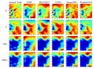
Figure 9: Visualization of Bias-Correction on Ningbo Dataset. Each row corresponds to a meteorologic factor and each column corresponds to an algorithm.

Factor-wise graphs. Fig. 10 shows an example of the learned factor-wise graphs. Grid 500 locates in the mountains and Grid 2555 is in the ocean. 10ws and 100ws at both grids are closely related to each other. However, 10ws of Grid 500 is more relevant to pressure, as the mountainous regions have diverse terrain and are prone to rapid changes in air pressure, resulting in great effects on wind speeds. On the other hand, 10ws of Grid 2555 is affected by 10div (10m horizontal divergence, a measure of the local spreading or divergence of wind field in a horizontal plane at the height of 10 meters). One of the possible reasons is that on sea horizon, the expansion of air in the horizontal direction has a significant impact on wind speed.

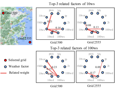
Figure 10: The Illustration of Learned Factor-Wise Graphs of Two Grids on Two Different Types of Terrains.

Hierarchical structure. Fig. 11 presents the clustering assignment of the hierarchical structure based on meteorologic and geographic distance on the Ningbo dataset. The comprehensive hierarchical structure can effectively cluster even for geographically non-adjacent grids, such as the range covered by the super-grid indicated in red at level 3.

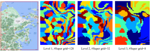
Figure 11: The Plot of Hierarchical Structure Based on Meteorologic and Geographic Distance of the Ningbo Dataset.

Dynamic adjustment of spatial dependencies. Fig. 12 gives an example of how the spatial weights change within a super-grid of the Ningxia dataset. Fig. 12(a) is the geometric distribution of grids. Our hierarchical design clusters the grids of local plains between the hills into a super grid. We present the spatial dependencies of these grids in Fig. 12(b). Fig. 12(c) and (d) are two samples chosen from the test set of the Ningxia dataset. On the one hand, the dynamic adjustment can adapt to the changing nature of NWP, on the other hand, the dynamic adjustments still preserve the strong spatial dependencies, such as the relationships determined by proximity (see in red circle).

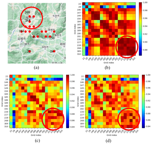
Figure 12: The Adjusted Spatial Dependencies within a Super-Grid of the Ningxia dataset.

Appendix F F. Blustery weather

WeatherGNN has the potential to model extreme weather (i.e., long-tail weather events exhibiting singular spatio-temporal patterns), as the dynamic adjustment module can adaptively learn data-dependent dependencies. In Fig. 13, we can find WeatherGNN performs well in blustery weather, which can be considered as generalized extreme weather.

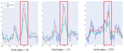
Figure 13: Bias-correction of wind speed at 10m in the blustery weather on the Ningbo datasets.

Appendix G G. Model Interpretability

WeatherGNN captures both meteorologic interactions with factor-wise GNN. By analyzing the edge weights in the learned factor-wise graphs, we can identify the most relevant factors for each factor. WeatherGNN learns 2726 factor graphs for all 2726 grids in Ningbo Dataset. By averaging the weights between 10ws and other factors in the 2726 factor graphs, we can identify the top 5 relevant factors for 10ws, which are wind speed at 10m (10ws), wind speed at 100m (100ws), wind direction at 10m (10wd), wind direction at 100m (100wd), and pressure (p). If we divide the terrain into land and sea based on altitude, we can observe that the top 5 relevant factors for 10ws on land are 10ws, 100ws, 10wd, 100wd, and p, while those at sea are 10ws, 100ws, 10wd, 100wd, and 10div (10m horizontal divergence, a measure of the local spreading or divergence of wind field in a horizontal plane at the height of 10 meters). These interesting phenomena can be explained by the fact that land areas have diverse terrain and are susceptible to rapid changes in air pressure, which greatly affects wind speeds. On the sea, the expansion of air in the horizontal direction has a significant impact on wind speed. The two specific cases of learned factor-wise graphs shown in Fig. 10 in the paper further verify this finding.

By analyzing the degree of centrality of nodes in the learned spatial graph, we can identify which corresponding grids are the most important or influential. On the Ningbo dataset, the top 10 central grids are Grid 398, 1399, 257, 1493, 1446, 1947, 304, 351, 1902, and 1901. These grids are crucial for maintaining the overall performance of the model, as removing them results in a significant decrease in accuracy. Upon further analysis, we observe that the most important grids are clustered in the estuary (orange circle) and mountain (yellow circle) regions (see the left part of Fig. 14). This observation is consistent with the distribution of wind speeds in the region, as shown in the right part of Fig. 14. These two wind speed cases are selected from EarthWindMap(https://earth.nullschool.net/) corresponding to the validation period of the Ningbo dataset. It can be seen that the wind speed at the estuary is often larger (brighter color) compared to other grids in Ningbo, while the wind speed near mountains is often smaller (darker color). When atmospheric motion changes significantly, the differences in wind speed at these locations become more pronounced, thereby highlighting the importance of these grids.

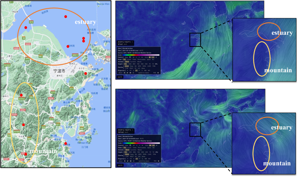
Figure 14: Left side: Top influential grids for the wind speed bias-correction on the Ningbo dataset. Most grids are clustered in the estuary (orange circle) and mountain (yellow circle) regions. Right side: Two wind speed cases selected from EarthWindMap corresponding to the validation period of the Ningbo dataset. The wind speed at the estuary is larger (brighter color) than other grids, while the wind speed near mountains is smaller (darker color).

References

- Bai et al. (2020) Bai, L.; Yao, L.; Li, C.; Wang, X.; and Wang, C. 2020. Adaptive graph convolutional recurrent network for traffic forecasting. In Advances in Neural Information Processing Systems, 17804–17815.
- Bauer, Thorpe, and Brunet (2015) Bauer, P.; Thorpe, A.; and Brunet, G. 2015. The quiet revolution of numerical weather prediction. Nature, 525(7567): 47–55.
- Bi et al. (2023) Bi, K.; Xie, L.; Zhang, H.; Chen, X.; Gu, X.; and Tian, Q. 2023. Accurate medium-range global weather forecasting with 3D neural networks. Nature, 1–6.
- Cai, Yao, and Chen (2021) Cai, D.; Yao, A.; and Chen, Y. 2021. Dynamic normalization and relay for video action recognition. Advances in neural information processing systems, 34: 11026–11040.
- Cai et al. (2019) Cai, Y.; Ge, L.; Liu, J.; Cai, J.; Cham, T.-J.; Yuan, J.; and Thalmann, N. M. 2019. Exploiting spatial-temporal relationships for 3D pose estimation via graph convolutional networks. In Proceedings of the IEEE/CVF international conference on computer vision, 2272–2281.
- Chen et al. (2023a) Chen, K.; Han, T.; Gong, J.; Bai, L.; Ling, F.; Luo, J.-J.; Chen, X.; Ma, L.; Zhang, T.; Su, R.; et al. 2023a. FengWu: Pushing the Skillful Global Medium-range Weather Forecast beyond 10 Days Lead. arXiv preprint arXiv:2304.02948.
- Chen et al. (2023b) Chen, L.; Zhong, X.; Zhang, F.; Cheng, Y.; Xu, Y.; Qi, Y.; and Li, H. 2023b. FuXi: A cascade machine learning forecasting system for 15-day global weather forecast. arXiv preprint arXiv:2306.12873.
- Chen et al. (2020) Chen, W.; Chen, L.; Xie, Y.; Cao, W.; Gao, Y.; and Feng, X. 2020. Multi-range attentive bicomponent graph convolutional network for traffic forecasting. In Proceedings of the AAAI Conference on Artificial Intelligence, 3529–3536.
- Chen, Gel, and Poor (2022) Chen, Y.; Gel, Y.; and Poor, H. V. 2022. Time-conditioned dances with simplicial complexes: Zigzag filtration curve based supra-hodge convolution networks for time-series forecasting. Advances in Neural Information Processing Systems, 35: 8940–8953.
- Dosovitskiy et al. (2020) Dosovitskiy, A.; Beyer, L.; Kolesnikov, A.; Weissenborn, D.; Zhai, X.; Unterthiner, T.; Dehghani, M.; Minderer, M.; Heigold, G.; Gelly, S.; et al. 2020. An image is worth 16x16 words: Transformers for image recognition at scale. arXiv preprint arXiv:2010.11929.
- Gao et al. (2022) Gao, Z.; Shi, X.; Wang, H.; Zhu, Y.; Wang, Y. B.; Li, M.; and Yeung, D.-Y. 2022. Earthformer: Exploring space-time transformers for earth system forecasting. Advances in Neural Information Processing Systems, 35: 25390–25403.
- Ge et al. (2022) Ge, T.; Pathak, J.; Subramaniam, A.; and Kashinath, K. 2022. DL-Corrector-Remapper: A grid-free bias-correction deep learning methodology for data-driven high-resolution global weather forecasting. arXiv preprint arXiv:2210.12293.
- Gneiting and Raftery (2005) Gneiting, T.; and Raftery, A. E. 2005. Weather forecasting with ensemble methods. Science, 310(5746): 248–249.
- Guibas et al. (2021a) Guibas, J.; Mardani, M.; Li, Z.; Tao, A.; Anandkumar, A.; and Catanzaro, B. 2021a. Adaptive fourier neural operators: Efficient token mixers for transformers. arXiv preprint arXiv:2111.13587.
- Guibas et al. (2021b) Guibas, J.; Mardani, M.; Li, Z.; Tao, A.; Anandkumar, A.; and Catanzaro, B. 2021b. Efficient Token Mixing for Transformers via Adaptive Fourier Neural Operators. In International Conference on Learning Representations.
- Guo et al. (2021) Guo, K.; Hu, Y.; Sun, Y.; Qian, S.; Gao, J.; and Yin, B. 2021. Hierarchical Graph Convolution Network for Traffic Forecasting. Proceedings of the AAAI Conference on Artificial Intelligence, 35(1): 151–159.
- Guo et al. (2019) Guo, S.; Lin, Y.; Li, S.; Chen, Z.; and Wan, H. 2019. Deep spatial–temporal 3D convolutional neural networks for traffic data forecasting. IEEE Transactions on Intelligent Transportation Systems, 20(10): 3913–3926.
- Han et al. (2021) Han, L.; Chen, M.; Chen, K.; Chen, H.; Zhang, Y.; Lu, B.; Song, L.; and Qin, R. 2021. A deep learning method for bias correction of ECMWF 24–240 h forecasts. Advances in Atmospheric Sciences, 38(9): 1444–1459.
- Han et al. (2022) Han, Y.; Mi, L.; Shen, L.; Cai, C.; Liu, Y.; Li, K.; and Xu, G. 2022. A short-term wind speed prediction method utilizing novel hybrid deep learning algorithms to correct numerical weather forecasting. Applied Energy, 312: 118777.
- Hu et al. (2021) Hu, S.; Xiang, Y.; Huo, D.; Jawad, S.; and Liu, J. 2021. An improved deep belief network based hybrid forecasting method for wind power. Energy, 224: 120185.
- Jiang et al. (2023) Jiang, R.; Wang, Z.; Yong, J.; Jeph, P.; Chen, Q.; Kobayashi, Y.; Song, X.; Suzumura, T.; and Fukushima, S. 2023. MegaCRN: Meta-Graph Convolutional Recurrent Network for Spatio-Temporal Modeling. arXiv:2212.05989.
- Karim et al. (2022) Karim, M. M.; Li, Y.; Qin, R.; and Yin, Z. 2022. A dynamic Spatial-temporal attention network for early anticipation of traffic accidents. IEEE Transactions on Intelligent Transportation Systems, 23(7): 9590–9600.
- Kipf and Welling (2016) Kipf, T. N.; and Welling, M. 2016. Semi-supervised classification with graph convolutional networks. arXiv preprint arXiv:1609.02907.
- Lam et al. (2022) Lam, R.; Sanchez-Gonzalez, A.; Willson, M.; Wirnsberger, P.; Fortunato, M.; Pritzel, A.; Ravuri, S.; Ewalds, T.; Alet, F.; Eaton-Rosen, Z.; et al. 2022. GraphCast: Learning skillful medium-range global weather forecasting. arXiv preprint arXiv:2212.12794.
- Li et al. (2022) Li, Y.; Tang, F.; Gao, X.; Zhang, T.; Qi, J.; Xie, J.; Li, X.; and Guo, Y. 2022. Numerical weather prediction correction strategy for short-term wind power forecasting based on bidirectional gated recurrent unit and XGBoost. Frontiers in Energy Research, 9: 1014.
- Liu et al. (2022) Liu, M.; Zeng, A.; Chen, M.; Xu, Z.; Lai, Q.; Ma, L.; and Xu, Q. 2022. SCINet: time series modeling and forecasting with sample convolution and interaction. Advances in Neural Information Processing Systems, 35: 5816–5828.
- Liu et al. (2021) Liu, Z.; Lin, Y.; Cao, Y.; Hu, H.; Wei, Y.; Zhang, Z.; Lin, S.; and Guo, B. 2021. Swin transformer: Hierarchical vision transformer using shifted windows. In Proceedings of the IEEE/CVF international conference on computer vision, 10012–10022.
- Luo and Yuille (2019) Luo, C.; and Yuille, A. L. 2019. Grouped spatial-temporal aggregation for efficient action recognition. In Proceedings of the IEEE/CVF International Conference on Computer Vision, 5512–5521.
- Maraun (2016) Maraun, D. 2016. Bias correcting climate change simulations-a critical review. Current Climate Change Reports, 2(4): 211–220.
- Moran and Moran (2009) Moran, J. M.; and Moran, J. M. 2009. Weather Studies : Introduction to Atmospheric Science. Boston, MA: American Meteorological Association, 4th edition.
- Müller (2007) Müller, M. 2007. Dynamic time warping. Information retrieval for music and motion, 69–84.
- Nguyen et al. (2023) Nguyen, T.; Brandstetter, J.; Kapoor, A.; Gupta, J. K.; and Grover, A. 2023. ClimaX: A foundation model for weather and climate. arXiv preprint arXiv:2301.10343.
- Pathak et al. (2022) Pathak, J.; Subramanian, S.; Harrington, P.; Raja, S.; Chattopadhyay, A.; Mardani, M.; Kurth, T.; Hall, D.; Li, Z.; Azizzadenesheli, K.; et al. 2022. Fourcastnet: A global data-driven high-resolution weather model using adaptive fourier neural operators. arXiv preprint arXiv:2202.11214.
- Rasp et al. (2023) Rasp, S.; Hoyer, S.; Merose, A.; Langmore, I.; Battaglia, P.; Russel, T.; Sanchez-Gonzalez, A.; Yang, V.; Carver, R.; Agrawal, S.; et al. 2023. WeatherBench 2: A benchmark for the next generation of data-driven global weather models. arXiv preprint arXiv:2308.15560.
- Shi et al. (2015) Shi, X.; Chen, Z.; Wang, H.; Yeung, D.-Y.; Wong, W.-k.; and Woo, W.-c. 2015. Convolutional LSTM Network: A Machine Learning Approach for Precipitation Nowcasting. In Proceedings of the 28th International Conference on Neural Information Processing Systems, 802–810. MIT Press.
- Vazquez-Enriquez et al. (2021) Vazquez-Enriquez, M.; Alba-Castro, J. L.; Docío-Fernández, L.; and Rodriguez-Banga, E. 2021. Isolated sign language recognition with multi-scale spatial-temporal graph convolutional networks. In Proceedings of the IEEE/CVF Conference on Computer Vision and Pattern Recognition, 3462–3471.
- Wei et al. (2022) Wei, Y.; Liu, H.; Xie, T.; Ke, Q.; and Guo, Y. 2022. Spatial-temporal transformer for 3d point cloud sequences. In Proceedings of the IEEE/CVF Winter Conference on Applications of Computer Vision, 1171–1180.
- Wu et al. (2020) Wu, Z.; Pan, S.; Long, G.; Jiang, J.; Chang, X.; and Zhang, C. 2020. Connecting the dots: multivariate time series forecasting with graph neural networks. In Proceedings of the ACM SIGKDD International Conference on Knowledge Discovery & Spec- tral temporal graph neural network for multivariate time- series forecasting, 753–763.
- Yan et al. (2019) Yan, C.; Tu, Y.; Wang, X.; Zhang, Y.; Hao, X.; Zhang, Y.; and Dai, Q. 2019. STAT: Spatial-temporal attention mechanism for video captioning. IEEE transactions on multimedia, 22(1): 229–241.
- Yang et al. (2022) Yang, X.; Yang, S.; Tan, M. L.; Pan, H.; Zhang, H.; Wang, G.; He, R.; and Wang, Z. 2022. Correcting the bias of daily satellite precipitation estimates in tropical regions using deep neural network. Journal of Hydrology, 608: 127656.
- Yoshikane and Yoshimura (2022) Yoshikane, T.; and Yoshimura, K. 2022. A bias correction method for precipitation through recognizing mesoscale precipitation systems corresponding to weather conditions. PLoS Water, 1(5): e0000016.
- Yu, Yin, and Zhu (2018) Yu, B.; Yin, H.; and Zhu, Z. 2018. Spatio-temporal graph convolutional networks: A deep learning framework for traffic forecasting. In Proceedings of the International Joint Conference on Artificial Intelligence, 3634–3640.
- Zhang et al. (2019) Zhang, T.; Yan, P.; Li, Z.; Wang, Y.; and Li, Y. 2019. Bias-correction method for wind-speed forecasting. Meteorologische Zeitschrift, 28(4): 293–304.