Emergent chaotic iterations in hard sparse instances of hamiltonian path problem

Abstract

A hamiltonian path is a path walk $P$ that can be a hamiltonian path or hamiltonian circuit. Determining whether such hamiltonian path exists in a given graph $G=(V,E)$ is a NP-Complete problem. In this paper, a novel algorithm with chaotic behaviour for hamiltonian path problem is proposed. We show that our algorithm runs in $O(V^{5}(V+E))$ for hard sparse instances from FHCP challenge dataset.

1 Introduction

Contributions

In this paper, we provide a implementation of SFCM-R algorithm, which is, by our knowledge, the first algorithm that relies on emergent chaotic iterations to simulate a chaotic turing machine capable of finding hamiltonian path in a variety of hard instances of HCP in polynomial time/space, thus contributing for a better understanding of the hamiltonian path problem and NP-hard problems in general in the light of dynamical systems.

Diagnose Tools

In this paper, we use 0-1 test and Lyapunov expoent $\lambda$ and 0-1 test to test whether SFCM-R output is a dynamical chaotic system. Lyapunov expoent indicates chaos when $\lambda>0$ where nearby trajectories separate exponentially. The 0-1 test provides a single statistic, which approaches 1 for chaotic systems. Both take as input a time-series data of measurements $0\leq x\leq 1$ corresponding to difference degree between algorithm state and solution, where 0 is full similarity to solution.

2 Preliminary

Conventions

By convention, $v_{LABEL}$ is a vertex labelled as $v_{LABEL}$ and $N_{v_{LABEL}}(w)$ represents a set of vertices $w^{\prime}\in N(w)$ labelled as $v_{LABEL}$. $H^{\prime}_{\text{$v_{0}$}}$ is the root of $H^{\prime}\supseteq H$ and $H^{\prime}_{v}$ is the $v$ of its current state. The notation $H_{v_{LABEL}}$ represents a set of all vertices labelled as $v_{LABEL}$. Before continuing, we’ll briefly describe what each label means. Let $w$ be a vertex $w\in V$. If $w$ is an articulation point of $\tau\in\Omega$, it will labelled as $v_{A}$ or minimal articulation vertex. A vertex labelled as $v_{A}$ or $v_{L}$ is a $v_{B}$ vertex. For conciseness, Every real articulation point of $H$ is labelled as $v_{H}$ and $C_{\text{$v_{H}$}}=\text{$v_{H}$}\cup N(\text{$v_{H}$})$ represents a $C_{\text{$v_{H}$}}$ component.

Mathematical background

Let us denote by $[[a;b]]$ the following integers: ${a,a+1,...,b}$, where $a<b$. A system under consideration iteratively modifies a collection of $n$ components. Each component $i\in[[1;n]]$ takes its value $x_{i}$ among the domain $\mathbb{B}=\{0,1\}$. A configuration of the system at discrete time t is the vector $x^{t}=(x^{t}_{1},...,x^{t}_{n})\in\mathbb{B}^{n}$. The dynamics of the system is described according to a function $f=\mathbb{B}^{n}\to\mathbb{B}^{n}$ such that $f(x)=f_{1}(x),...,f_{n}(x))$. Let be given a configuration $x$. In what follows $N(i,x)=(x_{1},...,\overline{x}_{i},...,x_{n})$ is the configuration obtained by switching the $i$th component of $x$ ($\overline{x}_{i}$ is indeed the negation of $x_{i}$). Intuitively, $x$ and $N(i,x)$ are neighbours. The discrete iterations of $f$ are represented by the oriented graph of iterations $\Gamma(f)$.

In such graph, vertices are configurations of $\mathbb{B}^{n}$ and there is an arc labelled $i$ from $x$ to $N(i,x)$ is and only if $f_{i}(x)$ is $N(i,x)$. In the sequel, the strategy $S=(S^{t})^{t\in\mathbb{N}}$ is the sequence defining which component to update at time $t$ and $S^{t}$ denotes $i$th term. This iteration scheme that only modifies one element at each iteration is usually refereed to as asynchronous iterations. More precisely, we have for any $i$,$1\leq 1\leq n$.

$$\left\{\begin{array}[]{lr}x^{0}\in\mathbb{B}^{n},\\ x^{t+1}_{i}=\left\{\begin{array}[]{lr}f_{i}(x^{t})\text{ if }S^{t}=i,\in\mathbb{B}^{n},\\ x^{t+1}_{i}\text{ otherwise.}\end{array}\right.\end{array}\right.$$ (1)

Now, we show the link between asynchronous interations and Devaney’s chaos. We introduce the function $F_{f}$ that is defined for any given application $f:\mathbb{B}^{n}\to\mathbb{B}^{n}$ by $F_{f}:[[1;n]]\times\mathbb{B}^{n}\to\mathbb{B}^{n}$ such that:

$$F_{f}(s,x)_{j}=\left\{\begin{array}[]{lr}f_{j}(x)\text{ if }j=s\in\mathbb{B}^{n},\\ x_{j}\text{ otherwise. }\end{array}\right.$$ (2)

With such a notation, asynchronously obtained configurations are defined for times $t=0,1,2,...$ by:

$$\left\{\begin{array}[]{lr}x^{0}\in\mathbb{B}^{n}\text{ and }\\ x^{t+1}=F_{f}(S^{t},x^{t}).\end{array}\right.$$ (3)

Finally, iterations defined in Eq. 2 can be described by the following system,where $\sigma$ is the so-called shift function that removes the first term of the strategy (i.e., $S^{0}$).

$$\left\{\begin{array}[]{lr}x^{0}=((S^{t})^{t\in\mathbb{N}},x^{0})\in[[1;n]]^{\mathbb{N}}\times\mathbb{B}^{n},\\ x^{k+1}=G_{f}(X^{k}),\\ \text{ where }\displaystyle\left(((S^{t})^{t\in\mathbb{N}},x)\right)=\displaystyle\left(\sigma((S^{t})^{t\in\mathbb{N}},F_{f}(S^{0},x)\right).\par\end{array}\right.$$ (4)

The relation between $\Gamma(f)$ and $G_{f}$ is obvious: there exists a path from $x$ to $x^{\prime}$ in $\Gamma(f)$ if and only if there exists a strategy $s$ such that iterations of $G_{f}$ from the initial point $(s,x)$ reach the configuration $x^{\prime}$.

Theorem 1.

Let $f:\mathbb{B}^{n}\to\mathbb{B}^{n}$. Iterations of $G_{f}$ are chaotic according to Devaney if and only if $\Gamma(f)$ is strongly connected.

2.1 Chaotic iterations according to Devaney

In this section, we stablish the link between such iterations and Devaney’s chaos is finally presented at the end of this section. In what follows and for any function $f$,$f^{n}$ means that composition $f^{o}f^{o}...^{o}f$ ($n$ times) and an iteration of a dynamical system is the step that consists in updating the global state $x^{\prime}$ at time $t$ with respect to a function $f$ s.t. $x^{t+1}=f(x^{t})$. This definition consists of three conditions: topological transitivity, density of periodic points, and sensitive point dependence on initial conditions.

Topological transitivity

It’s checked when, for any point, any neighbourhood of its future evolution eventually overlap with any other given region. This property implies that a dynamical system cannot be broken into simpler subsystems. Intuitively, its complexity does not allow any simplification.

Density of periodic points

As chaos needs some regularity to ”counteracts” the effects of transitivity. In the Devaney’s formulation, a dense set of periodic points is the element of regularity that a chaotic dynamical system has to exhibit. We recall that a point $x$ is a periodic point for $f$ of periodic $n\in\textbf{N}^{*}$ if $f^{n}(x)=x$. Then, the map $f$ is regular on the topological space $(\chi,\tau)$ if the set of periodic points for $f$ is dense in $\chi$ (for any $x\in\chi$, we can find at least one periodic point in any of its neighbours. Thus, due to these two properties, two points close to each other can behave in a completely different manner, leading to unpredictability for the whole system.

Sensitive dependence on initial conditions

Let us recall that $f$ has sensitive dependence on initial conditions if there exists $\delta>0$ such that, for any $x\in\chi$ and any neighbourhood $V$ of $x$, there exist $y\in V$ and $n>0$ such that $(d(f^{n}(x),f^{n}(y))>\delta$. The value $\delta$ is called the constant of sensitivity of $f$.

2.2 Chaotic Turing Machines

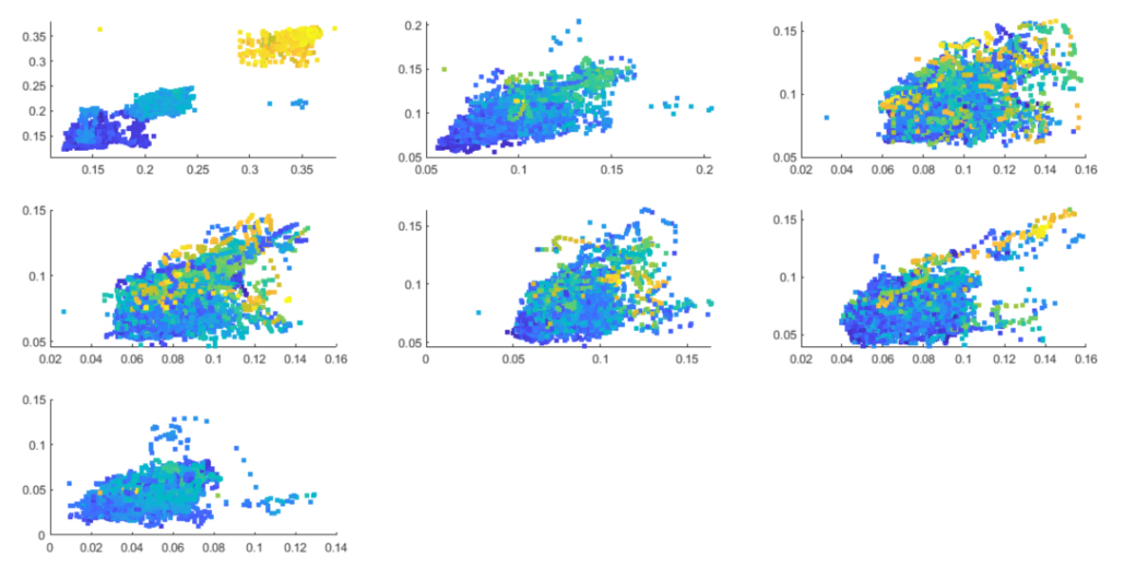
Figure 2: Reconstructed phrase space of signal $x_{i}=1-\frac{|x_{i}\cap L_{e}|}{|L_{e}|}$ from uniquely hamiltonian Fleischner graph - graph48. $x=0$ is the solution. Notice how Reconstruct approaches $x=0$ through chaotic iterations (from left to right). Each image corresponds to a different R-Policy rounds, from a total of 7 rounds. See section 4.

Let $(w,i,q)$ be the current configuration of the Turing machine (Figure 2), where $w=\#^{-\omega}(0)...w(k)\#^{\omega}$ is the paper tape, $i$ is the position of the tape head, $q$ is used for the state of the machine, and $\tau$ is its transition function (the notations used here are well-known and widely used). We define $f$ by:

$$f(w(0)...w(k),i,q)=(w(0)...w(i-1)aw(i+1)w(k),i+1,q^{\prime})$$ (5)

$$\text{ if }\tau(q,w(i))=(q^{\prime},a,\rightarrow)$$

$$f(w(0)...w(k),i,q)=(w(0)...w(i-1)aw(i-1)w(k),i+1,q^{\prime})$$ (6)

$$\text{ if }\tau(q,w(i))=(q^{\prime},a,\leftarrow)$$

Thus the Turing machine can be written as an iterate function $x^{n+1}=f(x^{n})$ on a well-defined set $\chi$, with $x^{0}$ as the initial configuration of the machine, which is $x^{0}=\{e_{i}=1:e\in L_{e}\}\vee\{e_{i}=0:e\notin L_{e}\}$ in our case. We denote by $\tau(S)$ the iterative process of the algorithm $S$. We show, experimentally, that our algorithm is capable of simulating a finite chaotic turing machine in a variety of hard instances of HCP with the emergence of chaotic iterations from its dynamics.

3 SFCM-R+ algorithm

3.1 Background

In this section, we present the first implementation of SFCM-R algorithm, called SFCM-R+, that relies on making the following conjecture hold, experimentally, for $H$ with a non-enforced parametrized polynomial-time runtime $log_{\varepsilon}V$.

Conjecture 1.

Let $H=(V,E,\text{$v_{0}$},L,\Omega)$ . $H$ has a hamiltonian sequence when (1) $|x^{t}_{k}\cap x^{t}_{m}|>0$ for every $z^{t}_{k}$, (2) $z^{t}_{m}$ maps a hamiltonian sequence, (3) $w^{*}=0$, (4) $\Gamma(f)$ is strongly connected.

$$w^{*}=g(z^{t},p)\text{ , }z^{t}=\displaystyle\left(\frac{|x^{t}_{k}\cap x^{t}_{m}|}{|x^{t}_{m}|}\right)^{m}_{k=i}$$ (7)

This is done by treating minimal mapping constraints as being part of a stable manifold of $g(z^{t},p)$, as the infinite number of unstable periodic orbits typically embedded in chaotic attractor could be taken advantage of for the purpose of achieving control by means of applying only very small perturbations in the system, which are related to enforcing ordering constraints progressively. By doing so, we can assume that there exists a nominal parameter value $p_{0}$, which is the desired orbit to be stabilized.

To every $x^{t}\in(x^{t}_{1},...,x^{t}_{n})$ we associate an analog cost function $K(s)\in[0,1]$ via $K(s=x^{t})=(max(\varepsilon(x^{t}))-min(\varepsilon(x^{t}))^{-1}\sum(\varepsilon(x^{t}_{i})-min(\varepsilon(x^{t}))$,$0\leq\varepsilon(w)\leq|V|$. Defining the energy function $V(s,\varepsilon)$ associated with $F=x^{t}$ via $V(s,a)=\sum^{M}_{m=1}=K_{m}(s)$, we see that as long as $a_{m}>0$,$\forall m\in\{1,...,M\}$ we have $V(s^{*})=0$ if and only if $s^{*}$ is a solution to F . Thus, we are looking for the lowest/zero energy points of $V$ by assuming that asynchronous iterations starting from $L_{e}$ leads to the formation of a global attracotr of the fixed point attractor $x^{*}$ where $V(s^{*})=0$, which corresponds to the solution. The search dynamics is as defined in is a gradient descent in $s$-space with a constrained ascent in the auxiliary $\varepsilon$-space.

$$\begin{array}[]{rcll}\displaystyle\frac{ds_{i}}{dt}=-\frac{\partial}{\partial s_{i}}V(\varepsilon,s),&&i=1,...,N\end{array}$$ (8)

We want to show that the dynamics is focused in the sense that the $x^{t}_{i}$ with the largest $K_{m}$ value violates the upper bound of energy of $V$, which is $\varepsilon_{MAX}$, and the dynamics drives exponentially fast to change such dominance until another $x^{t}_{i}$ happen to violates $\varepsilon_{MAX}$ and so on. Through experimentation, we show that the proposed system found at least one solution $s^{*}$ when one exists .

Here, $\Delta p$ cannot be changed directly as we can’t have access to $x^{t}_{m}$ until the reconstruction process is done. Because of that, the algorithm uses a local search scheme in order to change $\Delta p$ indirectly by solving the following optimization by using the functions Mapping and Reconstruct, respectively (see ref for details).

$${\begin{array}[]{rcll}\text{minimize}\hphantom{00}&&{\displaystyle F=\sum_{v\in V}\sum_{i=0}^{x}v_{\displaystyle i_{\varepsilon}}}\\[12.0pt] \text{subject to}\hphantom{00}&&0\leq v_{\displaystyle i_{\varepsilon}}\leq|V|\end{array}}$$ (9)

$${\begin{array}[]{rcll}\text{minimize}\hphantom{00}&&{\displaystyle\sum_{i=0}^{x}|H_{i}[V-v]_{\text{$v_{H}$}}|-|H_{i_{\text{$v_{A}$}}}\cap H_{i}[V-v]_{\text{$v_{H}$}}|}\\[12.0pt] \text{subject to}\hphantom{00}&&{\displaystyle H_{i_{\text{$v_{A}$}}}\cap H_{i}[V-v]_{\text{$v_{H}$}}\neq\emptyset}\end{array}}$$ (10)

$${\begin{array}[]{rcll}\text{maximize}\hphantom{00}&&{\displaystyle\sum_{i=0}^{x}|P^{i}_{x_{1}}|+|P^{i}_{x_{2}}|}\\[12.0pt] \text{subject to}\hphantom{00}&&{\displaystyle|P^{i}_{x_{1}}|+|P^{i}_{x_{2}}|\leq|V|}\end{array}}$$ (11)

The reconstruction process forms a continuous-time dynamical system. A continuous-time dynamical system as a deterministic algorithm does have these features: 1) the search happens on an energy landscape $V=\sum\varepsilon z^{t}$, 2) it solves easy problems efficiently (polynomial time, both analog and discrete) and 3) it guarantees to find solutions to hard problems even for solvable cases where many other algorithms fail. According to experimental analysis, although it is not a mathematically proved polynomial cost algorithm, it seems to find solutions in continuous-time t that scales polynomially on dataset, which is composed of a variety of hard HCP instances.

3.2 Reconstruction phrase

In this section, the reconstruction phrase is explained. The reconstruction task is done by the Reconstruct function, that takes following parameters as input by reference: $H=(V,E,\text{$v_{0}$},L,\Omega)$ , $L_{e}$, $H^{*}$, $\phi$, $P_{x_{1}}$, $P_{x_{2}}$. The edge $\phi$ is a non-synchronized edge $(x_{1}x_{2})\in L_{e}$ where $x_{1}$ and $x_{2}$ are initially the last vertices of two expandable paths $P^{\prime}=(x_{1})$ and $P^{\prime\prime}=(x_{2})$, respectively. $P_{x_{1}}=P^{\prime}$ will be the current path we’re expanding and $P_{x_{2}}=P^{\prime\prime}$, the other path. As for every $u$, $v$ must be added to either $P_{x_{1}}$ or $P_{x_{2}}$, $x_{1}$ and $x_{2}$ must be properly updated in order to represent the last vertices of $P_{x_{1}}$ and $P_{x_{2}}$, respectively. Every $H$ has the following property.

Property 1.

($|H^{n}|$ property) The property $|H^{n}|$ indicates that $H^{\prime}$ is a component of $H^{\prime}\supset H[V-H_{\text{$v_{H}$}}]$ has $n$ vertices $w\in Z$ with $Z=\{w^{\prime}\in V(H[V]):(|N(w)\cap H_{\text{$v_{H}$}}|=1)\wedge(w^{\prime}\neq\text{$v_{H}$})\}$. The value of $|H^{n}|$ is equal to $\alpha=\left|\bigcup_{w\in Z}\{N(w)\cap H_{\text{$v_{H}$}}\}\right|$; $|H_{\text{$v_{H}$}}^{n}|$ returns a set $\beta=\bigcup_{w\in Z}\{N(w)\cap H_{\text{$v_{H}$}}\}$. $|H^{n}|=0$ indicates that $H^{\prime}$ is a disconnected component of $H[V-H_{\text{$v_{H}$}}]$.

The term expansion call is used throughout this paper whenever we make a recursive call to Reconstruct. Every expansion call restores the initial state of both $H$ and $L_{e}$. Some conventions are used in this section. The synchronized edges will be written as $[v,u]$. The edge $[w,\square]$ is a synchronized edge $e\in L_{e}$ with $w\in e$.

Definition 1.

A synchronized edge is either: (1) a non-synchronized edge $(v,u)$ that got converted to $[v,u]$ by Reconstruct; or (2) an edge $[v,u]$ added to $L_{e}$ by Reconstruct.

The notation $d^{*}(x)$ is used to represent the degree of a vertex $x$ of a scene $H^{*}$, which is a clone of $H^{\prime}\supseteq H$ scene of the current state of Reconstruct, such that $V(H^{*})=V(H^{\prime})$ and $E(H^{*})=L_{e}\cap E(H^{\prime})$.

$P_{v}(u)$ function is used by Reconstruct to pass through $H$ by using paths of $H^{*}$, starting from $v\in\{x_{1},x_{2}\}$ until it reaches $z=u$ such that $d^{*}(z)=1$. During this process, it performs successive $H-v$ operation, converts edges from $(v,u)$ to $[v,u]$, and updates $P_{v}$. When $z$ is reached, it returns $z$. $[v,u]$ cannot be removed from $H$ unless by undoing operations performed by reconstruction phrase.

The goal of reconstruction phrase is to reconstruct a hamiltonian sequence (if it exists) by passing through $H$ in order to attach inconsistent $C_{\text{$v_{H}$}}$ components. If such hamiltonian sequence is reconstructed, $H^{*}$ will be a path graph corresponding to a valid hamiltonian sequence of the maximal $H\equiv G$. In order to do that, some edges may need to be added to $L_{e}$ to merge a component $H^{*}_{\prime}$ with $v\in V(H^{*}_{\prime})$ to another component $H^{*}_{\prime\prime}$ so that $P_{v}(u)$ can reach vertices $u\in V(H^{*}_{\prime\prime})$ properly. If this path graph is found, it means that exist a sequence of $C_{\text{$v_{H}$}}$ components that convert $L_{e}$ to a valid hamiltonian sequence. Such sequence is part of the forbidden condition of $A_{0}=SFCM-R$.

Definition 2.

Let $G=(V,E)$ be a graph. The Synchronization-based Forbidden Condition Mirroring (SFCM) algorithm is an algorithm with a configuration $g:W\times F\rightarrow A$, that consists of: (1) a finite set of scenes $W=W_{0}...W_{n}$,$W_{0}=G$, $W_{0}\equiv...\equiv W_{n}$, associated to each synchronizable forbidden condition in $F=F_{0}...F_{n}$; and (2) a pair $(w,f)$, with $w\in W$ and $f\in F$, associated to each mirrorable algorithm in $A=A_{0}...A_{n}$.

Definition 3.

(Synchronizable forbidden condition) If $F_{i}\in F$ and $F_{k}\in F$ don’t make the algorithms $A_{i}\in A$ and $A_{k}\in A$, respectively, fail to produce a valid output, then both $F_{i}\in F$ and $F_{k}\in F$ are synchronizable forbidden conditions that will be synchronized eventually when both $A_{i}$ and $A_{k}$ are executed.

In reconstruction phrase, a potential hamiltonian path $L_{e}$, which is the output of Mapping, is iteratively augmented by a local search scheme, one element at a time by Select-First. At each reconstruction iteration, $N(v)$ ordering can change depending on each $u^{x}\in N(v)$, $|\{e\in L_{e}:(u\in N(v))\wedge(u\in e)\}|$ and $d^{*}(u)$. $u^{x}$ is the priority of $u$, which is changed when $\varepsilon_{MAX}=\varepsilon_{u},V(s^{*})>0$. $N(v)$ ordering is changed by Reorder function, which returns $vN$. $vN$ is a set $S\supseteq N(v)$ In addition, $N(v)$ ordering can be changed by a shuffle operation before R-Policy reset the local priorities of reconstruction process in order to it not being stuck on local minimum. The current local search state is validated by Valid-state, that throws an error when one is found. This operations makes Reconstruct attempt to attach $\text{$v_{H}$}\in\textbf{{C}}$.

When a dead-end is found or every neighbour of $v$ is visited, we have $u=\textit{null}$. In this case,Path-split is called to change by reference $H$,$u$,$uN$,$vN$ and splitable. This function is called when $P_{x_{1}}$ reaches dead-end and $P_{x_{2}}$ needs to be expanded through $vN$ to reach another valid dead-end, or throw an error exception otherwise. $P_{x_{2}}$ is expanded by $P_{x_{1}=x_{2}}$, with (1) $(x_{1}x_{2})\in L_{e}$ or (2) $x_{2}\in V(H^{\prime})$,$H^{\prime}\in S_{1}$. If both (1) and (2) hold, or $P_{x_{2}}=\emptyset$, an error is thrown. After this operation,splitable is set to true. $vN$ is changed by Rec-Node, which takes $u$ and pass as parameter.

Algorithm 1 Reconstructor + R-Policy

1:$L_{e}$, $\phi$, hc, unrestrictedMode, hcp, longestPathFound

2:Set $L_{e}$ of synchronized edges

3:function Reconstruct

4:     $S\leftarrow(\emptyset)$

5:     $\textit{pass}\leftarrow\textit{true}$

6:     $vN\leftarrow\textsc{Rec-node}(x_{1},\textit{pass})$

7:     $u\leftarrow\textsc{Select-First}(vN)$

8:     while reconstruction of $L_{e}$ is not done do

9:         if $((u=\textit{null})\wedge\textit{splitable})$ then

10:              $u\leftarrow\textsc{Path-Swap}(H,vN)$          

11:         if $u=\textit{null}$ then

12:              throw expand          

13:         $u_{LAST}\leftarrow u$

14:         while $d^{*}(u)\neq 1$ do

15:              $vN\leftarrow\textsc{Rec-node}(u,\textit{pass})$

16:              try

17:                  if Valid-state($H$, C) then

18:                       $\textbf{{A}}\leftarrow\textbf{{C}}\cup\textbf{{A}}$

19:                       $\textbf{{C}}\leftarrow\emptyset$                                 

20:              catch error

21:                  $vN\leftarrow\textsc{Reorder}(N(v))$

22:                  Undo $k$ states until: (1) $|S|=1$ or

23:                  (2) $vN\sim w$, $w\in\textbf{{C}}$

24:                  $d^{*}(vN)\leftarrow 1$.               

25:              $u\leftarrow\textsc{Select-First}(vN)$

26:              if first then $V\leftarrow V\cup v$               

27:              if ($u\neq\textit{null}$) then

28:                  $vN\leftarrow\textsc{Rec-node}(u,\neg\textit{pass})$

29:                  $u\leftarrow\textsc{Select-First}(vN)$

30:              else

31:                  Path-split($H$,$u$,$uN$,$vN$, splitable)                        

32:         if $u_{LAST}^{i}=|V|$ then

33:              throw expand          

34:         if $x_{1}=\{\text{last visited }u\sim v\}$ then

35:              if $P_{x_{1}}=\emptyset$ then $vN\leftarrow\textsc{Rec-node}(x_{1},\textit{pass})$

36:                  if ($u\neq\textit{null}$) then

37:                       if $d^{*}(u)=1$ then

38:                           $vN\leftarrow\textsc{Rec-node}(u,\neg\textit{pass})$

39:                           $u\leftarrow\textsc{Select-First}(vN)$                                                                 

40:         Path-split($H$,$u$,$uN$,$vN$, splitable)

41:         if $|P_{x_{1}}|+|P_{x_{1}}|>\alpha$ then

42:              $\textit{longestPathFound}\leftarrow L_{e}$               

43:     return $L_{e}$

When pass = true, $vN$ corresponds to $u\in(v,u)$, $u^{x\geq 1}$, $(v,u)\in L_{e}$. Otherwise, $u\in(w,u)$, $w\neq v$, $w^{x\geq 1}$. The approach used by R-Policy to augment $L_{e}$ by local search is to find the $L_{e}$ of highest $a=|P_{x_{1}}|+|P_{x_{2}}|$ by using a well-structured dynamic in which global priorities and each $N(v),v\in V$ ordering is updated. In addition, the boolean variables hcp and restrictedMode are changed depending on specific criteria. When $\textit{restrictedMode}=\textbf{true}$, R-Policy makes Reconstruct attach only explicitly $C_{\text{$v_{H}$}}$ components. Otherwise, R-Policy makes Reconstruct attach both isolated components $H^{\prime}\supset H$ with $|H^{n}|=0$ and explicitly $C_{\text{$v_{H}$}}$ components. When $\textit{hcp}=\textbf{true}$, R-Policy makes Reconstruct enforce $L_{e}$ to be a hamiltonian circuit. Otherwise, it makes Reconstruct enforce $L_{e}$ to be a hamiltonian path. When the local priorities of reconstruction process are reset, $L_{e}$ is set to longestPathFound and the process starts again until it reaches the stop condition or a valid solution. In our case, the stop condition is (1) the maximum number of R-Policy runs with $L_{e}$ being from last R-Policy call parameter instead of Mapping, (2) $\textit{longestPathFound}=\textit{null}$ or (3) $\exists{v^{-1}}$. the priority $x$ of $w$ is represented by $w^{x}$. In this process, there may be some $w\in V$ with $d^{*}(w)=0$ that is included to $L_{e}$ in line 30 and 31. Notice that we use A, J, C in a slightly different manner from theoretical algorithm. A is used in a way that prioritizes $H_{\text{$v_{H}$}}$ sets found when the reconstruction of a hamiltonian circuit is enforced by Reconstruct with restrictedMode set to true initially. J is not explicitly enforced in Reconstruct. In this implementation, J is equivalent to $\textbf{{J}}=\{w\in V:w^{x<1}\}$ since $w^{x>1}$ tend to be visited first.

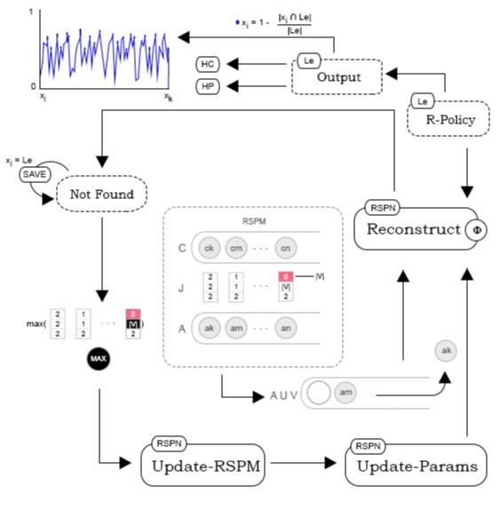
Figure 1: Reconstruction phrase steps

Algorithm 2 R-Policy Controller

1:$L_{e}$, $H=(V,E,\text{$v_{0}$},L,\Omega)$ , restrictedMode, hcp, longestPathFound, round

2:Set $L_{e}$ of synchronized edges

3:function R-Policy

4:     $\textit{lastLPF}\leftarrow\emptyset$

5:     $\textit{round}\leftarrow\textit{round}+1$

6:     $\textit{hc}\leftarrow hcp$

7:     for each $v\in V$ do

8:         Shuffle $N(v)$      

9:     while true do

10:         try

11:              $\phi\leftarrow\text{random non-visited }e\in L_{e}$

12:              if $\phi=\textit{null}$ then

13:                  throw notfound               

14:              $L_{e}\leftarrow$ Reconstruct($L_{e}$, $\phi$, hc, restrictedMode, hcp, longestPathFound)

15:              return $L_{e}$          

16:         catch expand

17:              try

18:                  $\phi\leftarrow\text{first non-visited }e_{v}e_{u}\in Z$ ,$e_{v}\in Z$,$Z=\{\textbf{{A}}\cup V\}$.

19:                  $|v\in V|_{\varepsilon}\leftarrow 0$

20:                  if $\phi=\textit{null}$ then

21:                       throw notfound                   

22:                  $L_{e}\leftarrow$ Reconstruct($L_{e}$, $\phi$, hc, restrictedMode, hcp, longestPathFound)

23:                  return $L_{e}$               

24:              catch notfound

25:                  $\textit{skip}\leftarrow\textit{false}$

26:                  for each $z$, $d^{*}(z)=0$ do

27:                       $d^{*}(z)\leftarrow c\in\{1,2\}$                   

28:                  $\textit{freqMax}\leftarrow max(|w|_{\varepsilon}^{T})$

29:                  $|v\in V|_{\varepsilon}^{T}=0$, $Z\leftarrow\emptyset$, $\textbf{{A}},\textbf{{C}}\leftarrow\emptyset$

30:                  if $\textit{freqMax}^{0}\wedge(d^{*}(freqMax)=2)$ then

31:                       Remove the first element of $S=\{L_{e}\cap(freqMax,\square)\}$ from $L_{e}$                   

32:                  if $\textit{longestPathFound}=\textit{null}$ then

33:                       return $L_{e}$                   

34:                  if $(\textit{step2}\wedge\neg\exists{v^{-1}})$ then

35:                       if ($|\textit{lastLPF}|>|\textit{longestPathFound}|$) then

36:                           if (restrictedMode) then

37:                                $\textit{freqMax}^{n}\leftarrow\textit{freqMax}^{n-1}$                            

38:                           if (hc) then

39:                                $\textit{restrictedMode}\leftarrow\textit{true}$

40:                           else

41:                                $\textit{restrictedMode}\leftarrow\textit{false}$                            

42:                           $\textit{skip}\leftarrow\textit{true}$

43:                           $\textit{hc}\leftarrow\textit{false}$                        

44:                       if  $(\neg\textit{skip})$ then

45:                           if (restrictedMode) then

46:                                $\textit{freqMax}^{n}\leftarrow\textit{freqMax}^{n-1}$

47:                                $\textit{restrictedMode}\leftarrow\textit{false}$

48:                           else

49:                                $L_{e}\leftarrow\textit{longestPathFound}$

50:                                $\textit{restrictedMode}\leftarrow\textit{true}$                                                                     

51:                  if $\exists{v^{-1}}$ then

52:                       return $L_{e}$

53:                  else

54:                       $\textit{lastLPF}\leftarrow\textit{longestPathFound}$                                          

55:         catch notfound

56:              return $L_{e}$               

In fact, when $w^{0}$, Reconstruct can’t even attach $w\in C_{\text{$v_{H}$}}$ by calling Valid-State. $w^{x}$ is changed when $|w|^{T}_{\varepsilon}>|V|$, $\varepsilon_{MAX}=|V|$. $|w|^{T}_{\varepsilon}$ is the accumulated error counter of $w$ through i-th expansion calls. $|w|_{\varepsilon}$ is the error counter of $w$ before an expansion call. Because of that, it is set to zero before an expansion call by $|v\in V|_{\varepsilon}\leftarrow 0$. When $|V|$ expansion calls are made, an exception is thrown and $N(v)$ is shuffled. Notice that by not shuffling $N(v)$ before each expansion call and by choosing only the first $u\in N(v)$ locally, we’re relying the capacity of the algorithm of reorganize itself to transform $L_{e}$ into a hamiltonian path in a deterministic, well-structured manner. Notice that the shuffle operation only affects the order of attachments, not the dynamics itself. We show in the experimental section that even by using a shuffling operation, the behaviour of Reconstruct is chaotic in variety of hard HCP instances. Instead, such operation seems to be crucial to make the algorithm converge to solution.

4 Experimental Analysis

In our experiments, we ran the above algorithm for 94 sparse graphs of FHCP dataset (sparse graphs with at most 558 vertices) with a time limit of 18 hours on AMD EPYC 7501 32-Core Processor, 8 GB RAM, 4 vCPU. Solution is found for 91 out of 94 graphs due to hardware limitations. The difference between Mapping output and solution state of Reconstruct until convergence, is seen downsampled in Figure 3 and 4. The resulting convergence of Reconstruct is seen in Figure 4, which is the state that represents the difference between Reconstruct state and solution state.

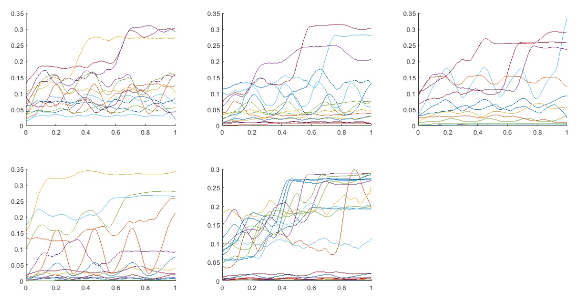
Figure 3: Mapping process - $w_{i}=1-\frac{|w_{i}\cap L_{e}|}{|L_{e}|}$

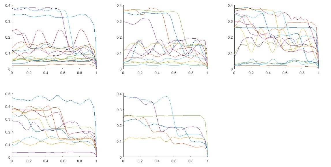
Figure 4: Reconstruct process - $x_{i}=1-\frac{|x_{i}\cap L_{e}|}{|L_{e}|}$

The following figure shows Lyapunov and $0-1$ test for $x_{i}=1-\frac{|x_{i}\cap L_{e}|}{|L_{e}|}$, respectively, of Reconstruct states (starting from Mapping output until convergence) for 91 graphs used above, indicating the presence of chaotic behaviour for almost all of them. These tests require a large number of datapoints to perform in a reliable manner. Because of that, these measurements are missing for a small fraction of instances, in which solution is found very fast, resulting in a very small $x_{i}=1-\frac{|x_{i}\cap L_{e}|}{|L_{e}|}$ . The resulting performance of algorithm is seen in Figure 5. The worst case scenario for tested graphs is $log_{|R_{\text{$v_{H}$}}|}V\cong 5$ or $O(V^{5}(V+E))$ for Reconstruct, and $log_{|M_{\text{$v_{H}$}}|}V\cong 2.5$ or $O(V^{2.5}(V+E))$ for Mapping (See supplementary material).

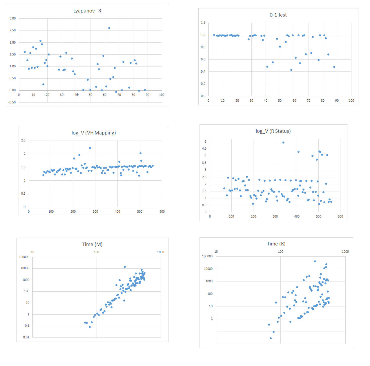
Figure 5: Lyapunov, 0-1 test, $log_{R_{|\text{$v_{H}$}|}}$, $log_{M_{|\text{$v_{H}$}|}}$, running time (in seconds) of mapping phrase , running time (in seconds) of reconstruction phrase

.

5 Conclusion

Our work shows emergent chaotic behaviour in hard instances of hamiltonian path problem. Elucidating the nature of NP-Complete problem is crucial to solve a variety of mathematical problems and can be promising for tackling real-world situations in which computational cost becomes a struggle.

6 Supplementary material

6.1 Path splitter

Algorithm 3 Path Splitter

1:$L_{e}$, $\phi$ hc, restrictedMode, hcp, longestPathFound

2:true

3:function Path-split

4:     if splitable then

5:         if hc then

6:              throw expand          

7:         $S\leftarrow\{H^{\prime}\supset H[V-H_{\text{$v_{H}$}}]:(|\{v\cup N(v)\cup x_{2}\cup N(x_{2})\}\cap V(H^{\prime})|=\emptyset)\wedge(0\leq|H^{n}|\leq 1)\}$

8:         $S_{0}\leftarrow\{H^{\prime}\in S:(|H^{n}|=1)\wedge(|H_{\text{$v_{H}$}}^{n}|^{x<1})\}$

9:         $S_{1}\leftarrow\{H^{\prime}\in S:|H^{n}|=0\}$

10:         if $((|S_{0}|>1)\vee(|S_{1}|>0))$ then

11:              throw expand          

12:         if ($S_{1}\neq\emptyset$) then

13:              $u^{\prime}\leftarrow u^{\prime}\in V(H^{\prime})$ with $H^{\prime}\in S_{1}$          

14:         if $((P_{x_{2}}=\emptyset)\wedge\neg\textit{splitable})$ then

15:              throw expand          

16:         if $H^{\prime}\in S_{1}$ then

17:              $vN\leftarrow\textsc{Rec-node}(u^{\prime},\textit{pass})$

18:         else

19:              $\textit{aux}=P_{x_{1}}$

20:              $P_{x_{1}}=P_{x_{2}}$

21:              $P_{x_{2}}=\textit{aux}$

22:              $vN\leftarrow\textsc{Rec-node}(x_{2},\textit{pass})$               

23:     $u\leftarrow\textsc{Select-First}(vN)$

24:     if $uN=\textit{null}$ then

25:         if $d^{*}(u)=1$ then

26:              $vN\leftarrow\textsc{Rec-node}(u,\neg\textit{pass})$

27:              $u\leftarrow\textsc{Select-First}(vN)$          

28:     else

29:         if splitable then

30:              $\textit{splitable}\leftarrow\textit{false}$

31:         else

32:              throw expand               

33:     return true

6.2 Validate state

Algorithm 4 Check if current state is valid

1:$v$, $H=(V,E,\text{$v_{0}$},L,\Omega)$

2:true

3:$\textit{iCounter}\leftarrow 0$

4:function Valid-state

5:     $X\leftarrow H_{\text{$v_{H}$}}$

6:     if $((P_{x_{2}}=\emptyset)\wedge\neg\textit{splitable})$ then

7:         throw expand      

8:     if (hc) then

9:         $S\leftarrow(x_{1}\in H_{\text{$v_{H}$}})\cup(x_{2}\in H_{\text{$v_{H}$}})$

10:         if $S\neq\emptyset$ then

11:              $\textbf{{C}}\leftarrow\textbf{{C}}\cup S$

12:              throw error               

13:     $V\leftarrow V-v$

14:     $S\leftarrow\{H^{\prime}\supset H[V-H_{\text{$v_{H}$}}]:(|\{v\cup N(v)\cup x_{2}\cup N(x_{2})\}\cap V(H^{\prime})|=\emptyset)\wedge(0\leq|H^{n}|\leq 1)\}$

15:     $S_{0}\leftarrow\{H^{\prime}\in S:(|H^{n}|=1)\wedge(|H_{\text{$v_{H}$}}^{n}|^{x<1})\}$

16:     $S_{1}\leftarrow\{H^{\prime}\in S:(|H^{n}|=1)\wedge(|H_{\text{$v_{H}$}}^{n}|^{x\geq 1})\}$

17:     $S_{2}\leftarrow\{H^{\prime}\in S:|H^{n}|=0\}$

18:     $S\leftarrow S_{0}\cup S_{1}\cup S_{2}$

19:     $\textit{valid}\leftarrow\textbf{true}$

20:     for each $H^{\prime}\in S$ do

21:         if $|H^{n}|=1$ then

22:              $\textit{ignore}\leftarrow\textbf{false}$

23:              if $|H_{\text{$v_{H}$}}^{n}|^{x<1}$ then

24:                  $\textit{iCounter}\leftarrow\textit{iCounter}+1$               

25:              if $((\textit{iCounter}>1)\wedge(|H_{\text{$v_{H}$}}^{n}|^{x<1}))$ then

26:                  $\textit{ignore}\leftarrow\textbf{true}$               

27:              if $(((\neg\textit{ignored})\wedge(|H_{\text{$v_{H}$}}^{n}|^{x<1}))\vee|H_{\text{$v_{H}$}}^{n}|^{x\geq 1})$ then

28:                  $|H_{\text{$v_{H}$}}^{n}|_{\varepsilon}\leftarrow|H_{\text{$v_{H}$}}^{n}|_{\varepsilon}+1$

29:                  $|H_{\text{$v_{H}$}}^{n}|_{\varepsilon}^{T}\leftarrow|H_{\text{$v_{H}$}}^{n}|_{\varepsilon}^{T}+1$

30:                  $V\leftarrow V\cup v$

31:                  if $|H_{\text{$v_{H}$}}^{n}|_{\varepsilon}>|V|$ then

32:                       $|H_{\text{$v_{H}$}}^{n}|_{\varepsilon}=0$

33:                       throw expand                   

34:                  $\textbf{{C}}\leftarrow\textbf{{C}}\cup|H_{\text{$v_{H}$}}^{n}|\cup V(H^{\prime})$

35:                  $\textit{valid}\leftarrow\textbf{false}$               

36:         else if $|H^{n}|=0$ then

37:              $\textbf{{C}}\leftarrow\textbf{{C}}\cup V(H^{\prime})$

38:              $\textit{valid}\leftarrow\textbf{false}$          

39:         $V\leftarrow V\cup v$

40:         if $(\neg\textit{valid})$ then

41:              if ($\neg\textit{restrictedMode}$) then

42:                  $\textbf{{C}}\leftarrow X$               

43:              throw error               

44:     return valid

6.3 Create reconstruction node

Algorithm 5 Create $vN$ node

1:$v$, pass

2:vN

3:function Rec-node

4:     if $v=-1$ then

5:         throw expand

6:     else

7:         $S_{L_{e}}\leftarrow\{e\in L_{e}:(u\in N(v))\wedge(u\in e)\wedge(u^{x\geq 1})\}$

8:         $S_{L_{e}}\leftarrow\{e\in S_{L_{e}}:(v\in e)\wedge(((v\notin e)\wedge\neg\textit{pass}))\vee((v\in e)\wedge\textit{pass})))\}$

9:         $S_{1}\leftarrow\{e\in S_{L_{e}}:(d^{*}(u)=1)\wedge(u\in e)\}$

10:         $S_{2}\leftarrow\{e\in S_{L_{e}}:(d^{*}(u)=2)\wedge(u\in e)\}$

11:         $S_{0}\leftarrow\{e\in E:(d^{*}(u)=0)\wedge(u\notin S_{L_{e}})\wedge(u\in e)\wedge(u^{x\geq 1})\}$

12:         $vN\leftarrow S_{1}\cup S_{2}\cup S_{0}$      

13:     return $vN$

6.4 Reorder N(v)

Algorithm 6 Reorder $N(v)$

1:$N(v)$ by reference

2:$S$

3:function Re-order

4:     $S\leftarrow\{v\in N(v):v\text{ is non-visited}\}$

5:     Order every $v\in S$ by $v_{\varepsilon}$

6:     $S\leftarrow\{v\in S:v^{x}=v^{x\geq 1}\}\cup\{v\in S:v^{x}=v^{x<1}\}$

7:     return $S$

6.5 Path swap

Algorithm 7 Path swap

1:$vN$,$H$,$P_{x_{1}}$,$P_{x_{2}}$ by reference

2:$u$

3:function Path-swap

4:     $P_{x_{2}}=P_{x_{2}}\cup\{x_{2}\}$

5:     $vN\leftarrow\textsc{Rec-node}(x_{2},\textit{pass})$

6:     $\textit{aux}=P_{x_{1}}$

7:     $P_{x_{1}}=P_{x_{2}}$

8:     $P_{x_{2}}=\textit{aux}$

9:     $u=\textsc{Select-First}(vN)$

10:     $\textit{splitable}\leftarrow\textit{false}$

11:     return $u$

6.6 Node selector

Algorithm 8 Select first $u$

1:$vN$,$H$,$P_{x_{1}}$,$L_{e}$

2:$u$

3:function Select-first($vN$)

4:     $V\leftarrow V-v$

5:     $u\leftarrow\text{first }w\in vN$

6:     if $(v,u)\notin L_{e}$ then

7:         if $d^{*}(u)>1$ then

8:              $L_{e}\leftarrow L_{e}-(\text{non-visited }e=\{w^{\prime},u)\})$          

9:         if $d^{*}(v)>1$ then

10:              $L_{e}\leftarrow L_{e}-(\text{non-visited }e=\{w^{\prime\prime},v\})$          

11:         $L_{e}\leftarrow L_{e}\cup(v,u)$      

12:     $P_{x_{1}}\leftarrow P_{x_{1}}\cup\{u\}$

13:     return $u$

6.7 FHCP dataset

In this section, the results of FHCP dataset is presented. $M_{|}VH|$ is the number of times articulation point is calculated in Mapping phrase. $R_{|}VH|$ is the number of times articulation point is calculated in Reconstruct phrase. $M_{\varepsilon}$ represents the number of errors of Mapping phrase. $R_{\varepsilon}$ represents the number of errors of Reconstruct phrase. $HC$ stands for hamiltonian cycle. $HP$ stands for hamiltonian path.

Instance	SFCM-R+
$H$	$V$	$E$	$M_{|\text{$v_{H}$}|}$	$R_{|\text{$v_{H}$}|}$	$\mu_{x}$	$M_{\varepsilon}$	$R_{\varepsilon}$	$log_{M_{|\text{$v_{H}$}|}}V$	$log_{R_{|\text{$v_{H}$}|}}V$	$L_{e}$
graph1	66	99	0	264	95.161	156	1203	1,692877851	1,205315549	HC
graph2	70	106	0	0	100.00	285	0	1,204175754	1,330468521	HC
graph3	78	117	0	23	96.104	287	190	1,204355003	1,299026958	HP
graph4	84	127	0	12450	81.944	395	52486	2,452888991	1,349386814	HP
graph5	90	135	0	234	98.864	415	1079	1,552018969	1,339674111	HP
graph6	94	142	0	262	98.889	401	956	1,510524463	1,319298376	HP
graph7	102	153	44	293	92.929	668	1363	1,560537483	1,406340845	HP
graph8	108	163	0	19742	75.556	593	80749	2,413238824	1,363736745	HP
graph9	114	171	0	578	96.429	720	2469	1,64933302	1,389141795	HP
graph10	118	178	0	10550	91.071	344	52827	2,27950044	1,224277461	HP
graph11	126	189	0	724	99.187	586	3281	1,673993305	1,317813955	HP
graph12	132	199	0	25939	73.451	797	106999	2,37170685	1,368242002	HP
graph13	138	207	0	536	99.265	952	2195	1,56150623	1,391965073	HP
graph14	142	214	0	59	97.872	1184	274	1,132631959	1,427946079	HP
graph15	150	225	0	9605	95.27	483	60756	2,198248421	1,233379859	HC
graph16	156	235	14	23918	77.612	1168	74125	2,220559976	1,398663279	HP
graph17	162	243	3	2547	97.468	512	15962	1,902266913	1,226183096	HC
graph18	166	250	0	865	99.387	1607	3213	1,579612607	1,444080986	HP
graph19	170	390	54	178880	82.468	1098	431358	2,526324545	1,363224376	HP
graph20	174	261	0	769	99.419	1666	3317	1,57137607	1,437895194	HP
graph21	180	271	0	33460	70.779	1577	148764	2,29351346	1,417935831	HP
graph22	186	279	0	32	99.454	1884	408	1,150317371	1,443076545	HP
graph23	190	286	0	35	83.333	895	239	1,043727545	1,29536736	HC
graph24	198	297	0	1	99.492	2332	24	0,600963191	1,466355897	HP
graph25	204	307	696	33	98.995	17311	657	1,219920578	1,835065291	HP
graph26	210	315	0	31	99.517	2327	479	1,15421292	1,449818452	HP
graph27	214	322	0	18	93.659	2311	178	0,965674005	1,443434631	HC
graph28	222	333	0	462	96.804	1511	4080	1,538839298	1,354981326	HP
graph29	228	343	1880	50569	73.196	42885	274546	2,306516284	1,964560395	HP
graph30	234	351	10	40	96.552	1100	705	1,202165311	1,283712784	HC
graph31	238	358	46	514	90.129	5277	2304	1,414842665	1,5662809	HC
graph32	246	369	0	539	99.588	3396	4111	1,51152052	1,47681452	HP
graph33	252	379	110	31979	98.785	8181	225024	2,228794718	1,629385155	HP
graph34	258	387	0	1	99.609	3385	68	0,759866453	1,46356354	HP
graph35	262	394	0	2	99.231	3955	190	0,942295159	1,487468291	HP
graph36	270	405	0	216	98.885	2219	1700	1,32865718	1,376247089	HP
graph37	276	415	16483	65798	74.684	276396	316957	2,253668679	2,229305382	HP
graph38	282	423	0	1995	97.491	2286	10000	1,632487075	1,370912131	HP
graph39	286	430	0	1539	99.648	4778	5589	1,52556014	1,497841159	HP
graph40	294	441	0	960	99.659	5212	3703	1,445725919	1,505867655	HP
graph41	300	451	0	77867	75.697	4416	429150	2,273852806	1,471477853	HP
graph42	306	459	81	54	99.016	7442	610	1,120531772	1,557571828	HP
graph43	310	466	0	0	100.000	5172	112	0,822529313	1,490613958	HC
graph44	318	477	0	840	99.684	5867	4570	1,46254657	1,505904431	HP
graph45	324	487	0	109997	74.17	4974	664378	2,319183771	1,472471422	HP
graph46	330	495	0	103	99.696	1731	1647	1,277218898	1,285796762	HP
graph47	334	502	169	92	74.545	2984	836	1,157884247	1,376841479	HP
graph48	338	776	594	7,88E+11	97.612	5175	3,36E+12	4,953243132	1,468577575	HP
graph49	342	513	0	18	99.11	1703	700	1,122757983	1,275130765	HC
graph50	348	523	0	120365	75.51	5919	614744	2,277597408	1,484214332	HP
graph51	354	531	0	2	99.43	3553	148	0,851415825	1,392934744	HP
graph52	358	538	0	6	97.159	3575	271	0,952654944	1,391322942	HC
graph53	366	549	0	1	99.725	7790	70	0,719762689	1,518067553	HP
graph54	372	559	0	106058	74.516	6776	583811	2,243211807	1,490336278	HP
graph55	378	567	0	1371	99.733	7946	7170	1,495841483	1,513156535	HP
graph56	382	574	3	1466	75.532	2169	12995	1,593212755	1,292090504	HP
graph57	390	585	0	3997	99.742	8493	19536	1,656012604	1,516388713	HP
graph58	396	595	273	166848	77.848	8514	774169	2,26694641	1,512931027	HP
graph60	402	603	0	3484	99.749	9047	20936	1,659185348	1,519263117	HP
graph61	406	610	0	175	99.012	10028	1173	1,176640744	1,533898559	HP
graph62	408	936	3858	613735	76.8	29031	1,57E+11	4,288532001	1,709476422	HP
graph63	414	621	0	4709	74.817	2369	97387	1,906190423	1,289478266	HP
graph64	416	625	3	205491	51.338	1351	591838	2,20389353	1,195320271	HP
graph65	420	631	44	121867	72.571	9580	705717	2,229536705	1,517722896	HP
graph66	426	639	0	892	99.764	4987	5731	1,429305807	1,406338278	HP
graph67	430	646	0	873	96.262	10947	18619	1,621419213	1,533830834	HC
graph68	438	657	0	485	98.391	10860	4629	1,387667275	1,527870294	HP
graph69	444	667	9	135208	72	10059	835950	2,236994182	1,511891122	HP
graph70	450	675	0	2	99.553	5511	174	0,844466561	1,410075669	HP
graph71	454	682	3	0	100.00	12460	241	0,896487381	1,541374464	HC
graph73	462	693	0	5561	99.782	12230	49826	1,762884495	1,533949587	HP
graph75	468	703	0	162209	74.807	10113	943591	2,237540705	1,499816956	HP
graph76	471	1161	361	2,01E+11	70.759	4284	48100000000	3,996281903	1,358705969	HP
graph77	474	711	0	975	99.788	13473	7596	1,450263983	1,54327593	HP
graph78	478	718	0	0	100.00	13518	179	0,840796289	1,541714352	HC
graph80	486	729	0	1233	99.376	3143	8235	1,457459519	1,301755813	HC
graph81	492	739	7	172639	75.545	12258	11700000000	3,740087808	1,518749115	HP
graph82	496	745	0	212552	74.949	1527	787511	2,187459362	1,181176287	HP
graph83	498	747	0	224	99.798	14919	1453	1,172412581	1,547417436	HP
graph85	502	754	0	1	99.799	14465	37	0,580664111	1,540457182	HP
graph86	503	1241	28225	1,87E+11	81.002	296899	4,77E+11	4,322866737	2,02571572	HP
graph88	507	1251	2352	1,69E+11	77.459	51870	3,44E+11	4,264888908	1,743032301	HP
graph89	510	765	0	1	99.803	15614	148	0,801553265	1,54881089	HP
graph91	516	775	0	208087	74.941	13550	1,24E+11	4,089515015	1,523211527	HP
graph92	522	783	0	576	99.808	16174	7315	1,421884782	1,548685698	HP
graph93	526	790	0	2	99.618	16456	82	0,703353135	1,549557651	HP
graph94	534	801	0	14855	74.953	3827	338949	2,0275163	1,313585433	HP
graph95	540	811	0	196188	73.789	14544	1,27E+11	4,063764119	1,523456804	HP
graph97	546	819	0	1	99.816	17940	115	0,752850862	1,554082227	HP
graph99	550	826	0	5	98.903	12894	310	0,909135752	1,499942939	HP
graph100	558	837	0	9	98.022	18623	111	0,744665227	1,554648102	HP

References

- [1] Lima C (2019). SFCM-R: A novel algorithm for the hamiltonian sequence problem. arXiv preprint arXiv:1902.06713v4
- [2] BAHI, Jacques M. et al. Neural networks and chaos: Construction, evaluation of chaotic networks, and prediction of chaos with multilayer feedforward networks. Chaos: An interdisciplinary Journal of Nonlinear Science, v. 22, n.1, 2012.