Modulating near-field thermal transfer through temporal drivings: a quantum many-body theory

Abstract

The traditional approach to studying near-field thermal transfer is based on fluctuational electrodynamics. However, this approach may not be suitable for nonequilibrium states due to dynamic drivings. In our work, we introduce a theoretical framework to describe the phenomenon of near-field heat transfer between two objects when subjected to periodic time modulations. We utilize the machinery of nonequilibrium Green’s function to derive general expressions for the DC energy current in Floquet space. Furthermore, we also obtain the energy current under the condition of small driving amplitude. The external drivings create a nonequilibrium state, which gives rise to various effects such as heat-transfer enhancement, heat-transfer suppression, and cooling. To illustrate these phenomena, we conduct numerical calculations on a system of Coulomb-coupled quantum dots, and specifically investigate the scenario of periodically driving electronic reservoir. In our calculations, we employ the $G_{0}W_{0}$ approximation, which does not require self-consistent iteration and is suitable for weak Coulomb interaction. Our theoretical formalism can be applied to study near-field energy transfer between two metallic plates under periodic time modulations.

I Introduction

Near-field heat transfer between objects with nanoscale separations has recently received significant attention due to its potential in energy harvesting and thermal management applications [1, 2, 3, 4, 5, 6, 7]. The theoretical treatment is typically formulated within the framework of fluctuating electrodynamics, which is based on the fluctuation-dissipation theorem by assuming a thermal equilibrium state for each object [8, 9]. This approach allows for the calculation of the near-field thermal current between objects, taking into account their geometries, material properties, and the frequency and polarization of the electromagnetic fields involved [6].

Recently, there has been a growing interest in the use of temporal modulation as a promising approach to control and manage thermal radiation [10, 11, 12, 13, 14, 15, 16, 17, 18, 19, 20, 21, 22, 23]. In the near-field regime, Latella et al. reported on the shuttling effect between two bodies with an oscillating temperature differences or photon chemical potential difference. However, it is important to note that this work assumes the two bodies are always in thermal equilibrium [11]. Other recent studies have focused on the time modulation of resonance frequencies to generate synthetic electric and magnetic fields [19, 20, 21]. These studies have reported nonreciprocity in the heat transfer transmission function using quantum Langevin equations. It is worth mentioning that the validity of the fluctuation-dissipation theorem has been assumed under certain conditions. Furthermore, the manipulation of spatial coherence in thermal radiation has been achieved by using a time-modulated lossless layer on top of a semi-infinite lossy substrate [17, 18]. The time modulation enables the spatial-coherence transfer and correlations between different frequency components. A quantum theoretical formulation, based on macroscopic quantum electrodynamics, has been proposed by assuming that the time-varying susceptibility modulation is local in time [22]. This theory predicts several nontrivial effects, including nonlocal correlations between fluctuating currents, far-field thermal radiation surpassing the black-body spectrum, and quantum vacuum amplification effects.

In addition to the traditional theoretical formalism based on fluctuational electrodynamics [9], a fully quantum theoretical framework utilizing the nonequilibrium Green’s function (NEGF) has been established to calculate the near-field heat current mediated by charge fluctuations [24, 25, 26, 27, 28, 29, 30]. In this work, we start from the microscopic Hamiltonian and extend the NEGF formalism to study near-field energy transfer in the presence of periodic time modulations. We derive general expressions for the energy current in the Floquet space without relying on the fluctuation-dissipation theorem. Additionally, we expand the energy current up to the second order of the driving amplitude. Using numerical calculations, we demonstrate several effects induced by the driving, such as heat-transfer enhancement, heat-transfer suppression, and cooling in a system consisting of Coulomb-coupled quantum dots.

The paper is structured as follows. In Sec. II, the model Hamiltonian and the derivation of the energy currents from two perspectives are presented. Some of the details are provided in the appendices. In Sec. III, we discuss the specific scenario of small driving amplitude. Section IV is devoted to the numerical results of the system of Coulomb coupled quantum dots, along with their physical interpretations. Our work is summarized in Sec. V.

II Theoretical Formalism

II.1 System and Hamiltonian

We investigate the near-field heat transfer between two objects by considering the contribution from charge fluctuations, as shown in Fig. 1. The energy transport between the two subsystems which are separated by a vacuum gap is mediated by electromagnetic field. To facilitate energy transport, the electronic reservoirs which serve as the heat baths in the subsystems are explicitly considered in the theoretical formalism. This will become clear later when we derive the expression of the energy current. The total Hamiltonian of the open quantum system can be partitioned as

$$\hat{H}_{\rm tot}=\hat{H}_{e}+\hat{H}_{\phi}+\hat{H}_{e\phi}.$$ (1)

The electronic Hamiltonian is given by

$$\hat{H}_{e}=\sum_{\alpha}\big{(}\hat{H}_{\alpha}+\hat{H}_{\alpha B}+\hat{V}_{\alpha B}+\hat{V}^{\dagger}_{\alpha B}\big{)},$$ (2)

where $\alpha=L,R$ denotes the two subsystems [See Fig. 1]. In the tight-binding model, the Hamiltonian of object $\alpha$ is

$$\hat{H}_{\alpha}=\sum_{i,j\in\alpha}h_{ij}c_{i}^{\dagger}c_{j},$$ (3)

where $i$ and $j$ run over all the electronic sites of object $\alpha$. The electronic reservoir which provides the dissipation channel for the energy current is considered in the Hamiltonian $\hat{H}_{\alpha B}$ with

$$\hat{H}_{\alpha B}=\sum_{k}\epsilon_{k\alpha}d_{k\alpha}^{\dagger}d_{k\alpha}.$$ (4)

The coupling between object $\alpha$ and its corresponding reservoir is given by

$$\hat{V}_{\alpha B}=\sum_{k,i\in\alpha}t_{k\alpha,i}d_{k\alpha}^{\dagger}c_{i},$$ (5)

which means that an electronic reservoir is attached to every site of the object. The degrees of freedom of the reservoirs can be analytically integrated out and act as self-energies in the electronic Green’s functions. Both $\hat{H}_{\alpha}$ and $\hat{H}_{\alpha B}$ can be time-dependent, depending on the problems to study. In our numerical calculation in Sec. IV, we drive $\hat{H}_{\alpha B}$ by applying an AC voltage bias to the electronic reservoir. To drive the object Hamiltonian $\hat{H}_{\alpha}$ via time-dependent electromagnetic fields, the Peierls substitution which ensures the gauge invariance is used. This substitution adds a scalar potential to the diagonal term and also introduces a vector potential as a phase factor in the hopping matrix elements with [31]

$$h_{ij}(t)=\big{[}h_{ij}-e_{0}\varphi(\bm{r}_{i},t)\delta_{ij}\big{]}\exp\Big{[}\frac{ie_{0}}{\hbar}\int_{\bm{r}_{i}}^{{\bm{r}_{j}}}d\bm{r}\cdot\bm{A}(\bm{r},t)\Big{]}.$$ (6)

Here, $\bm{r}_{i}$ represents the coordinates of electronic site $i$ and $e_{0}$ denotes the elementary charge. The time-periodic scalar potential $\varphi(\bm{r},t)$ can be achieved by applying a gate voltage to semiconductor nanostructures, such as quantum dots and quantum wires. In the case of two-dimensional metallic materials, the scalar potential (or carrier density) can be dynamically modulated using all-optical techniques [32, 33]. Additionally, the time-periodic vector potential $\bm{A}(\bm{r},t)$ can be realized by applying circularly polarized light.

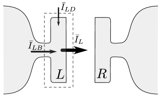
Figure 1: Schematic plot of the near-field energy transfer between two objects by considering charge fluctuations. The two subsystems where the electronic reservoirs serving as the heat baths are explicitly shown are denoted by $L$ and $R$. The average energy current flowing out of heat bath $\alpha$ is denoted as $\bar{I}_{\alpha B}$ with $\alpha=L,R$. With the external driving applied to object $\alpha$ (driving Hamiltonian $\hat{H}_{\alpha}$), the average energy current pumped into the object is $\bar{I}_{\alpha D}$. There is a conservation of energy current being expressed as $\bar{I}_{\alpha}=\bar{I}_{\alpha B}+\bar{I}_{\alpha D}$. It should be noted that if the driving is only applied to the bath Hamiltonian $\hat{H}_{\alpha B}$, we have $\bar{I}_{\alpha}=\bar{I}_{\alpha B}$.

In the context of near-field energy transfer, retardation effects due to the finite speed of propagation of electromagnetic fields can be disregarded. As a result, we do not need to consider the vector potential arising from the transverse component of the fluctuating electric currents, which is responsible for the far-field thermal radiation. Instead, our focus is on the scalar potential caused by the longitudinal fluctuating electric currents [24, 34, 35, 36, 37, 38, 29]. The observation that the Coulomb interaction is the primary mechanism for near-field heat transfer between metals was first made by Mahan [34].

The traditional approach to studying the Coulomb interaction involves eliminating the scalar field and focusing on the instantaneous interaction. However, in this work, we consider the scalar field as a fundamental quantum operator and define it in terms of the usual NEGF method [24, 29]. This approach allows us to treat the Green’s functions for electrons [as shown in Eqs. (12) and (14)] and the scalar Coulomb field [as shown in Eq. (26)] on an equal footing. Moreover, it also facilitates discussing the symmetry properties of the Green’s functions [see Appendix C]. The Hamiltonian of the scalar Coulomb field $\phi$ is given by [39]

$$\hat{H}_{\phi}=-\frac{\epsilon_{0}}{2}\int d\bm{r}\left[\big{(}\dot{\phi}(\bm{r})\big{)}^{2}/c_{0}^{2}+\big{(}\nabla\phi(\bm{r})\big{)}^{2}\right].$$ (7)

Here, $\epsilon_{0}$ is the vacuum permittivity. Due to the instantaneous nature of the Coulomb interaction, the scalar field $\phi$ does not have a free field dynamics and hence no conjugate momentum from the perspective of quantum field theory. Therefore, a fictitious speed of light $c_{0}$ is introduced. We take $c_{0}$ to infinity at the end of the calculations. For further details, we refer to Ref. [29]. The Hamiltonian that describes the interaction between the Coulomb field and electronic charges is given by

$$\hat{H}_{e\phi}=-e_{0}\sum_{i}\rho_{i}\phi(\bm{r}_{i}),$$ (8)

where $\rho_{i}=c_{i}^{\dagger}c_{i}$ is the number operator at electronic site $i$ with coordinate $\bm{r}_{i}$, and $e_{0}$ represents the elementary charge. In the limit of $c_{0}\rightarrow\infty$, this theory is equivalent to the instantaneous Coulomb problem. The Hamiltonian $\hat{H}_{\phi}+\hat{H}_{e\phi}$ captures the electron-electron interaction expressed by $\sum_{i,j}v_{ij}c_{i}^{\dagger}c_{j}^{\dagger}c_{j}c_{i}/2$ with the interaction strength $v_{ij}=e_{0}^{2}/(4\pi\epsilon_{0}|\bm{r}_{i}-\bm{r}_{j}|)$.

Below we derive the expressions for the DC energy current from both the perspectives of electronic transport and Coulomb field. The equivalence between these two perspectives is proven in Appendix D and Appendix E. The main result is presented in Subsection II.C and Section III. One who is not interested in electronic transport can skip Subsection II.B without losing any coherence.

II.2 Perspective from the electronic transport

We start deriving our formalism from the perspective of electronic transport. The average energy current consists of two components: one flowing out of the electronic reservoir and the other pumped by the external drive [See Fig. 1]. The energy current flowing out of electronic reservoir $\alpha$ at time $t$ is calculated in the Heisenberg picture by

$$I_{\alpha B}(t)= \frac{1}{i\hbar}\left<\big{[}\hat{H}_{\rm tot}(t),\hat{H}_{\alpha B}(t)\big{]}\right>$$

$$= \frac{1}{i\hbar}\left<\big{[}\hat{V}_{\alpha B}(t)+\hat{V}^{\dagger}_{\alpha B}(t),\hat{H}_{\alpha B}(t)\big{]}\right>$$

$$= \sum_{k,i\in\alpha}\left<t_{k\alpha,i}\dot{d}_{k\alpha}^{\dagger}c_{i}+t^{*}_{k\alpha,i}c^{\dagger}_{i}\dot{d}_{k\alpha}\right>.$$ (9)

The ensemble average is defined as $\left<\cdots\right>=\rm{tr}(\hat{\rho}\cdots)$, where $\hat{\rho}$ is the density-matrix operator. The time evolution of $d_{k\alpha}^{\dagger}$ and $d_{k\alpha}$ is governed by the total Hamiltonian, as shown by

$$\big{[}d_{k\alpha}^{\dagger},\hat{H}_{\rm tot}\big{]}=\big{[}d_{k\alpha}^{\dagger},\hat{H}_{\alpha B}\big{]}-\sum_{i}t^{*}_{k\alpha,i}c^{\dagger}_{i},$$ (10)

$$\big{[}d_{k\alpha},\hat{H}_{\rm tot}\big{]}=\big{[}d_{k\alpha},\hat{H}_{\alpha B}\big{]}+\sum_{i}t_{k\alpha,i}c_{i}.$$ (11)

By plugging these equations into Eq. (II.2), the contributions from the second terms cancel with each other. It is worth mentioning that the expression of Eq. (II.2) in terms of electronic Green’s functions has been derived in many works before [40, 41, 29]. We provide a brief sketch of the derivation for completeness. By defining the following Green’s function on the Keldysh contour with

$$G_{i,k\alpha}(\tau,\tau^{\prime})=\frac{1}{i\hbar}\left<{\cal T}c_{i}(\tau)d^{\dagger}_{k\alpha}(\tau^{\prime})\right>,$$ (12)

where ${\cal T}$ is the contour time-ordering operator, the thermal current can be expressed using the lesser component $G^{<}_{i,k\alpha}$ as

$$I_{\alpha B}(t)=-i\hbar\sum_{k,i\in\alpha}\Big{[}t_{k\alpha,i}\partial_{t^{\prime}}G^{<}_{i,k\alpha}(t,t^{\prime})\Big{]}\Big{|}_{t^{\prime}=t}+{\rm c.c.}.$$ (13)

In this work, the time variables in Greek letters sit on the Keldysh contour while those in Latin letters are normal ones. We can express $G_{i,k\alpha}$ in terms of the Green’s functions of object $\alpha$ and the corresponding isolated electronic reservoir, $G_{ij}$ and $g_{k\alpha}$, respectively, as

$$G_{i,k\alpha}(\tau,\tau^{\prime})=\sum_{j}\int d\tau_{1}G_{ij}(\tau,\tau_{1})t^{*}_{k\alpha,j}g_{k\alpha}(\tau_{1},\tau^{\prime}).$$ (14)

Using the Langreth rule [42], the energy current $I_{\alpha B}(t)$ can be expressed as

$$I_{\alpha B}(t)=-i\hbar\int_{-\infty}^{\infty} dt^{\prime}{\rm tr}\Big{[}G_{\alpha}^{r}(t,t^{\prime})\partial_{t}\Sigma_{\alpha}^{<}(t^{\prime},t)$$

$$+ G_{\alpha}^{<}(t,t^{\prime})\partial_{t}\Sigma_{\alpha}^{a}(t^{\prime},t)\Big{]}+{\rm c.c.}.$$ (15)

Here, the entries of $G_{\alpha}$ and $\Sigma_{\alpha}$ are respectively, $G_{ij}$ and $\Sigma_{ij}$ with $\Sigma_{ij}(\tau,\tau^{\prime})=\sum_{k}t^{*}_{k\alpha,i}g_{k\alpha}(\tau,\tau^{\prime})t_{k\alpha,j}$. The superscripts $<$, $r$, and $a$ denote the lesser, retarded, and advanced components, respectively. In this work, the symbol ${\rm tr}$ denotes trace over electronic sites only. Note that the time derivatives are on the electronic self-energies, and the positions are important for the driven case.

We map to the Floquet space, which is explained in more detail in Appendix A. Using Eqs. (A.12) and (A.13), the DC component $\bar{I}_{\alpha B}\equiv\int_{0}^{T}dtI_{\alpha B}(t)/T$ with period $T=2\pi/\Omega$ is

$$\bar{I}_{\alpha B}=\int_{\rm BZ}\frac{dE}{\pi\hbar}{\rm Re}\Big{[}{\rm Tr}\Big{(}\bm{E}\bm{G}_{\alpha}^{r}\bm{\Sigma}_{\alpha}^{<}+\bm{E}\bm{G}_{\alpha}^{<}\bm{\Sigma}_{\alpha}^{a}\Big{)}\Big{]},$$ (16)

where the symbol ${\rm Tr}$ denotes trace over both the electronic sites and the Floquet spaces. It is a generalization of the Meir-Wingreen formula [40, 43] for the energy transport in Floquet space under periodic modulation. Here and below, we use the boldface letters to denote the matrices in Floquet space. The entries of matrices $\bm{E}$ and $\bm{F}$ are, respectively, $E_{m}\delta_{m,n}$ and $F_{mn}$ with $E_{m}=E+m\hbar\Omega$. Note that the integration region is restricted to the “first Brillouin zone” with $-\hbar\Omega/2<E\leq\hbar\Omega/2$, which is denoted as “BZ”. Equation (16) gives the energy current flowing out of electronic reservoir $\alpha$. It is applicable in cases where the electronic reservoir or the object are periodically driven, or both are driven.

In the scenario where the external drive is applied to object $\alpha$ represented by $\hat{H}_{\alpha}$, the energy current pumped into system $\alpha$ is given by

$$I_{\alpha D}(t)=\sum_{ij\in\alpha}\dot{h}_{ij}(t)\big{<}c_{i}^{{\dagger}}(t)c_{j}(t)\big{>}=-i\hbar\ {\rm tr}\big{[}\dot{h}_{\alpha}(t)G_{\alpha}^{<}(t,t)\big{]}.$$ (17)

Using Eq. (D.6), the DC component becomes

$$\bar{I}_{\alpha D}=\frac{1}{T}\int_{0}^{T}i\hbar\ {\rm tr}\Big{\{}h_{\alpha}(t)\big{[}\partial_{t}G_{\alpha}^{<}(t,t)\big{]}\Big{\}}dt.$$ (18)

Using Eqs. (A.11)-(A.13), we obtain its expression in the energy domain as

$$\bar{I}_{\alpha D}=\int_{\rm BZ}\frac{dE}{2\pi\hbar}{\rm Tr}\Big{(}\bm{h}_{\alpha}\big{[}\bm{E},\bm{G}_{\alpha}^{<}\big{]}\Big{)},$$ (19)

where $\bm{h}_{\alpha}$ is a Toeplitz matrix in the Floquet space with entries:

$$[\bm{h}_{\alpha}]_{lp}=\frac{1}{T}\int_{0}^{T}h_{\alpha}(t)e^{i(l-p)\Omega t}dt.$$ (20)

The total near-field energy current is the sum of $\bar{I}_{\alpha B}$ and $\bar{I}_{\alpha D}$.

II.3 Perspective from the Coulomb field

We can also derive the expression of the energy current from the energy density of the Coulomb field with

$$u=-\frac{\epsilon_{0}}{2}\left\{\big{[}\dot{\phi}(\bm{r})\big{]}^{2}/c_{0}^{2}+\big{[}\nabla\phi(\bm{r})\big{]}^{2}\right\}.$$ (21)

The conservation law in a differential equation form is obtained as [29]

$$\partial_{t}u =-\epsilon_{0}\left[\dot{\phi}\ddot{\phi}/c_{0}^{2}+\nabla\dot{\phi}\cdot\nabla\phi\right]$$

$$=-\nabla\cdot\bm{j}+e_{0}\sum_{i}\rho_{i}\dot{\phi}(\bm{r}_{i})\delta(\bm{r}-\bm{r}_{i}),$$ (22)

where we have set $c_{0}$ to infinity, defined the Poynting vector due to the Coulomb field as $\bm{j}=\epsilon_{0}\dot{\phi}\nabla\phi$, and used the Poisson equation $\nabla^{2}\phi(\bm{r})=e_{0}\sum_{i}\rho_{i}\delta(\bm{r}-\bm{r}_{i})/\epsilon_{0}$ with $e_{0}$ the elementary charge. By integrating over volume and using Gauss’s law, Eq. (II.3) can be rewritten as

$$\oint_{\alpha}\left<\bm{j}\right>\cdot d\bm{A}=e_{0}\sum_{i\in\alpha}\big{<}\rho_{i}\dot{\phi}(\bm{r}_{i})\big{>}-\int_{\alpha}\big{<}\partial_{t}u\big{>}d\bm{r},$$ (23)

where $\bm{A}$ is the surface that encloses object $\alpha$. The left-hand side describes the energy current mediated by the Coulomb field. The right-hand side consists of two terms: the first term describes Joule heating by longitudinal current, while the second term describes the energy change rate of the dynamical Coulomb field. They are respectively denoted as $I_{\alpha}(t)$ and $I_{\alpha d}(t)$. We also refer to $I_{\alpha d}$ as the displacement energy current. It is analogous to the displacement current in AC electronic transport [44, 45]. The displacement energy current only exists in the Coulomb field and does not involve any real energy transfer, which means that its DC component vanishes, i.e., $\bar{I}_{\alpha d}=0$. Therefore, the average energy current flowing out of an object is solely contributed by Joule heating.

In the time domain, the bare (unscreened) Coulomb potential $V$ satisfies

$$\epsilon_{0}\left(\frac{1}{c_{0}^{2}}\frac{\partial^{2}}{\partial t^{2}}-\nabla^{2}\right)V(\bm{r}t,\bm{r}^{\prime}t^{\prime})=e_{0}^{2}\delta(\bm{r}-\bm{r}^{\prime})\delta(t-t^{\prime}).$$ (24)

It is seen that $e_{0}^{2}V^{-1}=-\epsilon_{0}\nabla^{2}$ under $c_{0}\rightarrow\infty$. Using the Poisson equation $\nabla^{2}\phi(\bm{r})=e_{0}\sum_{i}\rho_{i}\delta(\bm{r}-\bm{r}_{i})/\epsilon_{0}$, we have

$$I_{\alpha}(t)= {\rm Re}\left\{\epsilon_{0}\int_{\alpha}d\bm{r}\left<\big{[}\nabla^{2}\phi(\bm{r}t^{\prime})\big{]}\dot{\phi}(\bm{r}t)\right>\Big{|}_{t^{\prime}=t}\right\}$$

$$= {\rm Re}\left\{i\hbar\int_{\alpha}d\bm{r}\big{[}V^{-1}\partial_{t}W^{<}(\bm{r}t,\bm{r}t^{\prime})\big{]}\big{|}_{t^{\prime}=t}\right\}.$$ (25)

which can be expressed in terms of the dynamically screened Coulomb potential defined on the Keldysh contour as

$$W(\bm{r}\tau,\bm{r}^{\prime}\tau^{\prime})=\frac{e_{0}^{2}}{i\hbar}\left<{\cal T}\phi(\bm{r}\tau)\phi(\bm{r}^{\prime}\tau^{\prime})\right>.$$ (26)

The dynamically screened Coulomb potential is related to the unscreened Coulomb potential $V$ and the polarization function $\Pi$ defined in Eq. (B.13) through the Dyson equation as shown in Eq. (B). Using Eqs. (A.11) and (A.13), the average of $I_{\alpha}(t)$ in the energy domain can be expressed as

$$\bar{I}_{\alpha}= {\rm Re}\left[\int_{\rm BZ}\frac{dE}{2\pi\hbar}{\rm Tr}_{\alpha}\big{(}\bm{E}\bm{V}^{-1}\bm{W}^{<}\big{)}\right]$$

$$= {\rm Re}\left[\int_{\rm BZ}\frac{dE}{2\pi\hbar}{\rm Tr}_{\alpha}\big{(}\bm{E}\bm{\Pi}^{<}\bm{W}^{a}+\bm{E}\bm{\Pi}^{r}\bm{W}^{<}\big{)}\right],$$ (27)

where Eq. (B.23) has been used to get the second identity. Equation (II.3) is one of the main results of this work. It is similar in form to Eq. (16) where $\bm{W}$ represents the Green’s function for the scalar field, analogous to the electronic Green’s function $\bm{G}$, and the polarization function $\bm{\Pi}$ corresponds to self-energy from electronic reservoir. The relation $\bar{I}_{\alpha}=\bar{I}_{\alpha B}+\bar{I}_{\alpha D}$ is proven in Appendix D and Appendix E. Using the symmetries in Eq. (C.2), we can alternatively express $\bar{I}_{\alpha}$ as

$$\bar{I}_{\alpha}=\frac{1}{2}\int_{\rm BZ}\frac{dE}{2\pi\hbar}{\rm Tr}_{\alpha}\Big{[}\bm{E}\bm{\Pi}^{<}\bm{W}^{a}+\bm{E}\bm{\Pi}^{r}\bm{W}^{<}-\big{(}\bm{\Pi}\leftrightarrow\bm{W}\big{)}\Big{]}.$$ (28)

III The case of small driving amplitude

To gain a more intuitive physical understanding, we consider the case where the driving amplitude is small. By considering up to the second order of the driving amplitude, the polarization function can be expanded as

$$\bm{\Pi}^{\gamma}_{\alpha}=\bm{\Pi}^{\gamma 0}_{\alpha}+\bm{\Pi}^{\gamma 1}_{\alpha}+\bm{\Pi}^{\gamma 2}_{\alpha},$$ (29)

with $\gamma=<,r,a$. Here, $\bm{\Pi}^{\gamma 0}_{\alpha}$ represents the polarization function in the absence of external driving. The drivings induce $\bm{\Pi}^{\gamma 1}_{\alpha}$ and $\bm{\Pi}^{\gamma 2}_{\alpha}$, which are proportional to the first and second order of the driving amplitude, respectively. Both $\bm{\Pi}^{\gamma 0}_{\alpha}$ and $\bm{\Pi}^{\gamma 2}_{\alpha}$ are diagonal in Floquet space. On the other hand, the term $\bm{\Pi}^{\gamma 1}_{\alpha}$ is tridiagonal and its value depends on the phase of the external driving. Using Eq. (B.23), the dynamically screened Coulomb potential is thus expanded as

$$\bm{W}^{\gamma}=\bm{W}^{\gamma 0}+\bm{W}^{\gamma 1}+\bm{W}^{\gamma 2}.$$ (30)

Therefore, in the case of small driving amplitude, the energy current flowing out of the part $L$ is expressed as

$$\bar{I}_{L}=\bar{I}_{L0}+\bar{I}_{L2}+\bar{I}_{L\theta}.$$ (31)

The zeroth-order contribution is given by

$$\bar{I}_{L0}={\rm Re}\bigg{\{}\int_{\rm BZ}\frac{dE}{2\pi\hbar}{\rm Tr}\big{[}\bm{E}\big{(}\bm{\Pi}_{L}^{<0}\bm{W}_{LL}^{a0}+\bm{\Pi}_{L}^{r0}\bm{W}_{LL}^{<0}\big{)}\big{]}\bigg{\}},$$ (32)

which represents the energy current in the absence of temporal driving. The term that is first order in driving amplitude vanishes. The second-order contribution consists of two terms, denoted as $\bar{I}_{L2}$ and $\bar{I}_{L\theta}$. The expression of $\bar{I}_{L2}$ is given by

$$\bar{I}_{L2}={\rm Re}\bigg{\{}\int_{\rm BZ}\frac{dE}{2\pi\hbar} {\rm Tr}\big{[}\bm{E}\big{(}\widetilde{\bm{\Pi}}_{L}^{<2}\bm{W}_{LL}^{a0}+\widetilde{\bm{\Pi}}_{L}^{r2}\bm{W}_{LL}^{<0}$$

$$+ \bm{\Pi}_{L}^{<0}\bm{W}_{LL}^{a2}+\bm{\Pi}_{L}^{r0}\bm{W}_{LL}^{<2}\big{)}\big{]}\bigg{\}},$$ (33)

with

$$\widetilde{\bm{\Pi}}_{\alpha}^{r2}=\bm{\Pi}_{\alpha}^{r2}+\bm{\Pi}_{\alpha}^{r1}\bm{W}_{\alpha\alpha}^{r0}\bm{\Pi}_{\alpha}^{r1},\quad\widetilde{\bm{\Pi}}_{\alpha}^{a2}=\Big{(}\widetilde{\bm{\Pi}}_{\alpha}^{r2}\Big{)}^{\dagger},$$ (34)

$$\widetilde{\bm{\Pi}}_{\alpha}^{<2}=\bm{\Pi}_{\alpha}^{<2}+\bm{\Pi}_{\alpha}^{<1}\bm{W}_{\alpha\alpha}^{a0}\bm{\Pi}_{\alpha}^{a1}+\bm{\Pi}_{\alpha}^{r1}(\bm{W}_{\alpha\alpha}^{<0}\bm{\Pi}_{\alpha}^{a1}+\bm{W}_{\alpha\alpha}^{r0}\bm{\Pi}_{\alpha}^{<1}),$$ (35)

$$\bm{W}_{LL}^{a2}=\bm{W}_{LL}^{a0}\widetilde{\bm{\Pi}}_{L}^{a2}\bm{W}_{LL}^{a0}+\bm{W}_{LR}^{a0}\widetilde{\bm{\Pi}}_{R}^{a2}\bm{W}_{RL}^{a0},$$ (36)

and

$$\bm{W}_{LL}^{<2}= \bm{W}_{LL}^{<0}\widetilde{\bm{\Pi}}_{L}^{a2}\bm{W}_{LL}^{a0}+\bm{W}_{LL}^{r0}\big{(}\widetilde{\bm{\Pi}}_{L}^{<2}\bm{W}_{LL}^{a0}+\widetilde{\bm{\Pi}}_{L}^{r2}\bm{W}_{LL}^{<0}\big{)}$$

$$+ \bm{W}_{LR}^{<0}\widetilde{\bm{\Pi}}_{R}^{a2}\bm{W}_{RL}^{a0}+\bm{W}_{LR}^{r0}\big{(}\widetilde{\bm{\Pi}}_{R}^{<2}\bm{W}_{RL}^{a0}+\widetilde{\bm{\Pi}}_{R}^{r2}\bm{W}_{RL}^{<0}\big{)}.$$ (37)

It is evident that $\bar{I}_{L2}$ remains finite as long as one of the electronic reservoir is subjected to periodic drivings. In the case where both electronic reservoirs are driven, it is independent of the phase difference between the drivings. As we will see in the later numerical calculation, this term is relevant to heat-transfer enhancement, heat-transfer suppression and cooling. The expression of $\bar{I}_{L\theta}$ is given by

$$\bar{I}_{L\theta}={\rm Re}\bigg{\{}\int_{\rm BZ}\frac{dE}{2\pi\hbar}{\rm Tr}\big{[}\bm{E}\big{(}\bm{\Pi}_{L}^{<1}\widetilde{\bm{W}}_{L}^{a1}+\bm{\Pi}_{L}^{r1}\widetilde{\bm{W}}_{L}^{<1}\big{)}\big{]}\bigg{\}},$$ (38)

with

$$\widetilde{\bm{W}}_{L}^{a1}=\bm{W}_{LR}^{a0}\bm{\Pi}_{R}^{a1}\bm{W}_{RL}^{a0},$$ (39)

and

$$\widetilde{\bm{W}}_{L}^{<1}=\bm{W}_{LR}^{<0}\bm{\Pi}_{R}^{a1}\bm{W}_{RL}^{a0}+\bm{W}_{LR}^{r0}\left(\bm{\Pi}_{R}^{<1}\bm{W}_{RL}^{a0}+\bm{\Pi}_{R}^{r1}\bm{W}_{RL}^{<0}\right).$$ (40)

The term $\bar{I}_{L\theta}$ is finite only when both reservoirs are driven and depends on the phase difference between the drivings.

IV Numerical Results

In this section, we present the numerical results for the system of Coulomb-coupled quantum dots with the Hamiltonian:

$$\hat{H}_{\alpha}=\epsilon_{\alpha}c_{\alpha}^{{\dagger}}c_{\alpha},$$ (41)

to demonstrate the physical implications of the periodic temporal modulation. We specifically focus on the case of driving the electronic reservoir with a small driving amplitude. We consider a sinusoidal drive, which can be described by $\epsilon_{k\alpha}=\epsilon_{0,k\alpha}+\varepsilon_{\alpha}(t)$, where $\varepsilon_{\alpha}(t)=\mu_{\alpha}\cos(\Omega t+\theta_{\alpha})$ with driving amplitude $\mu_{\alpha}$, driving angular frequency $\Omega$ and phase $\theta_{\alpha}$. This driving can be realized through an AC voltage bias applied to the electrode. The reservoir self-energy $\Sigma_{\alpha}^{\gamma}$ with $\gamma=<,r,a$ in the time domain is given by [41]

$$\Sigma_{\alpha}^{\gamma}(t_{1},t_{2})=\Sigma_{\alpha 0}^{\gamma}(t_{1}-t_{2})\exp\left[\frac{1}{i\hbar}\int_{t_{2}}^{t_{1}}\varepsilon_{\alpha}(t)dt\right],$$ (42)

with $\Sigma_{\alpha 0}^{\gamma}(t_{1}-t_{2})$ representing the self-energy in the absence of periodic drive and $\kappa_{\alpha}=\mu_{\alpha}/(\hbar\Omega)$. By using Eq. (A.8) and the Jacobi-Anger expansion $\exp(i\kappa\sin x)=\sum_{n}J_{n}(\kappa)\exp(inx)$ with $J_{n}$ the Bessel function of the first kind, we find

$$\big{[}\bm{\Sigma}^{\gamma}_{\alpha}(E)\big{]}_{mn}=e^{i(n-m)\theta_{\alpha}}\sum_{l}J_{m-l}(\kappa_{\alpha})J_{n-l}(\kappa_{\alpha})\Sigma_{\alpha 0}^{\gamma}(E_{l}).$$ (43)

In the wide-band limit, which assumes energy-independent tunneling rates between the quantum dots and the electronic reservoirs, we have $\Sigma_{\alpha 0}^{r/a}(E_{l})=\mp i\eta$ where $\eta$ is the half linewidth broadened by the electrode. Thus, the retarded and advanced self-energies are diagonal in Floquet space with

$$\big{[}\bm{\Sigma}^{r/a}_{\alpha}(E)\big{]}_{mn}=\mp i\eta\delta_{mn}.$$ (44)

The lesser component $\bm{\Sigma}^{<}_{\alpha}$ is obtained by noticing that $\Sigma_{\alpha 0}^{<}(E_{l})=2i\eta f_{\alpha,l}$, where the Fermi-Dirac distribution function is $f_{\alpha,l}=1/\{\exp[\beta_{\alpha}(E_{l}-\mu_{0})]+1\}$ with $\beta_{\alpha}=1/(k_{B}T_{\alpha})$. We consider the case where the driving amplitude is small, i.e., $\kappa_{\alpha}\ll 1$. Expanding to the second order of $\kappa_{\alpha}$ while maintaining a tridiagonal structure, one has

$$\big{[}\bm{\Sigma}^{<}_{\alpha} (E)\big{]}_{mn}=2i\eta\big{[}f_{\alpha,m}+(\kappa_{\alpha}^{2}/4)(f_{\alpha,m-1}+f_{\alpha,m+1})\big{]}\delta_{mn}$$

$$+i\kappa_{\alpha}\eta(f_{\alpha,m}-f_{\alpha,n})\big{(}e^{i\theta_{\alpha}}\delta_{m,n-1}-e^{-i\theta_{\alpha}}\delta_{m,n+1}\big{)}.$$ (45)

The electronic Green’s fucntions $\bm{G}_{0}^{r}$ and $\bm{G}_{0}^{<}$ are obtained through Eq. (B.21).

We use the $G_{0}W_{0}$ approximation [46] which requires no self-consistent iteration and is good for weak Coulomb interaction. Having obtained the Green’s functions $\bm{G}_{0}$, the polarization functions and dynamically screened Coulomb potentials are then calculated using Eqs. (B) and (B.23). In the numerical calculation, the quantum-dot levels are set as equal with $\epsilon_{L}=\epsilon_{R}=15\,$meV. The half linewidth broadened by the electronic reservoirs is $\eta=30\,$meV. The temperatures of the left and right reservoirs are $T_{L(R)}=T_{0}\pm\Delta T/2$ with $T_{0}=300\,$K. The driving frequency is given by $\hbar\Omega=5\,$meV. The Coulomb potential between the two quantum dots is set to be $20\,$meV. The parameters of the system under consideration are highly tunable. The quantum-dot levels and the coupling parameter $\eta$ can be experimentally controlled through gate voltages. The Coulomb potential is given by $v=e_{0}^{2}/(4\pi\epsilon_{\rm eff}d)$, where $d$ represents the effective distance between the dots and $\epsilon_{\rm eff}$ is the effective static dielectric constant, which depends on the physical properties of the quantum dots. It is important to note that the magnitude of the quantum dot levels, coupling parameter, and Coulomb potential do not influence the physics discussed below.

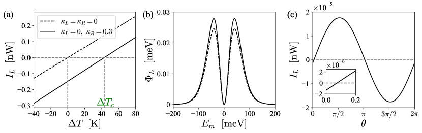
Figure 2: (a) The energy current $\bar{I}_{L}$ versus the temperature difference $\Delta T\equiv T_{L}-T_{R}$, with only electronic reservoir $R$ being driven. The energy current diminishes to zero at a finite $\Delta T$, denoted as $\Delta T_{c}$. The dashed line represents the case without any drivings, for comparison. (b) The spectrum function of the heat current is shown for a temperature difference of $\Delta T=40\,$K. The solid line represents the case where both electronic reservoirs are subjected to the same periodic driving, while the dashed line represents the case without any drivings. (c) In the absence of a temperature difference, the energy current versus the phase difference $\theta\equiv\theta_{L}-\theta_{R}$ is shown when both electronic reservoirs are subjected to periodic drivings with the same amplitude and frequency. The inset zooms in the curve at small $\theta$.

We begin by examining the scenario where only the electronic reservoir in part $R$ is driven with $\kappa_{R}=0.3$. Figure 2(a) illustrates the relationship between the energy current $\bar{I}_{L}$ and the temperature difference $\Delta T$. The energy current diminishes to zero at a certain positive $\Delta T$, referred to as $\Delta T_{c}$. When $\Delta T<0$ ($T_{R}>T_{L}$), the energy current is increased compared to the undriven case, indicating an enhancement in heat transfer. In the range of $0<\Delta T<\Delta T_{c}$, the energy current continues to flow from part $R$ to part $L$, suggesting active cooling of the lower temperature region. This implies that periodic temporal modulation presents a promising alternative for achieving near-field cooling effect [47, 48, 49, 7]. For $\Delta T>\Delta T_{c}$, the heat transfer is suppressed due to the periodic driving. The unequal energy-current magnitude by reversing the temperature difference allows for achieving thermal rectification effect. All of these phenomena are a result of the nonequilibrium state induced by the periodic driving.

We now investigate the scenario in which both electronic reservoirs are subjected to periodic drivings with the same amplitude and frequency. In the presence of a finite temperature difference, these drivings enhance the thermal transfer. The enhancement is mainly due to $\bar{I}_{L2}$, and the contribution from $\bar{I}_{LP}$ can be neglected in this case. The enhancement can be observed in Fig. 2(b), which depicts the energy current spectrum $\Phi_{L}$ defined as

$$\bar{I}_{L}=\int_{\rm BZ}\frac{dE}{2\pi\hbar}\sum_{m}\Phi_{L}(E,m).$$ (46)

When there is no temperature difference between the two parts, the energy current $\bar{I}_{L2}$ becomes zero. However, there is still a small but nonzero energy current $\bar{I}_{L\theta}$, as shown in Fig. 2(c). Notably, the energy current demonstrates periodicity with respect to the phase difference of the drivings, denoted as $\theta$. The finite negative energy current at $\theta=0$ suggests that energy is pumped into the system from the drivings.

V Conclusion

We have developed a theoretical framework using the nonequilibrium Green’s function method to investigate the near-field energy transport between two bodies when subjected to periodic temporal drivings. The energy current has been derived from both electronic transport and Joule heating, and the equivalence between these two perspectives has been demonstrated. In addition, we have expanded the energy current to the second order of the driving amplitude. The nonequilibrium state due to the external drivings is responsible for various effects including heat-transfer enhancement, heat-transfer suppression and cooling. These have been demonstrated numerically in a system of Coulomb-coupled quantum dots under $G_{0}W_{0}$ approximation. Our formalism can be extended to study more complex systems, such as the near-field energy transfer between two metallic plates where the electron densities are dynamially modulated.

Appendix A Floquet representation

We give a brief introduction to the Floquet representation of a function $F$ that has two independent arguments of time, $t_{1}$ and $t_{2}$ [50, 31, 51, 52]. By defining variables $t_{r}=t_{1}-t_{2}$ and $t_{a}=(t_{1}+t_{2})/2$, it is also possible to write in its Wigner form, $F^{w}$, as follows:

$$F(t_{1},t_{2})\equiv F^{w}(t_{a},t_{r}).$$ (A.1)

In equilibrium, $F$ only depends on $t_{r}$ because of continuous-time translational invariance. However, in the presence of a periodic drive, the system is out of equilibrium, causing $F$ to depend on both $t_{r}$ and $t_{a}$. Maintained by the discrete-time translational invariance, we have the following periodicity,

$$F(t_{1}+T,t_{2}+T)=F(t_{1},t_{2}),\ \ F^{w}(t_{a}+T,t_{r})=F^{w}(t_{a},t_{r}),$$ (A.2)

where $T$ is the period of the driving field.

The Wigner transformation of $F^{w}(t_{a},t_{r})$ into energy domain with energy $E$ and single integer index $l$ is given by

$$F^{w}_{l}(E)=\frac{1}{T}\int_{0}^{T}dt_{a}\int_{-\infty}^{\infty}dt_{r}e^{i(E/\hbar)t_{r}+il\Omega t_{a}}F^{w}(t_{a},t_{r}),$$ (A.3)

where $\Omega=2\pi/T$ is the driving angular frequency. The inverse transformation is

$$F^{w}(t_{a},t_{r})=\sum_{l\in\mathbb{Z}}\int_{-\infty}^{\infty}\frac{dE}{2\pi\hbar}e^{-i(E/\hbar)t_{r}-il\Omega t_{a}}F^{w}_{l}(E).$$ (A.4)

The Floquet representation of $F$ with Floquet indices $m$ and $n$ can be related to the Wigner representation via

$$F_{mn}(E)\equiv F^{w}_{m-n}\Big{(}E+\frac{m+n}{2}\hbar\Omega\Big{)}.$$ (A.5)

The range of $E$ in $F_{mn}(E)$ is limited to the “first Brillouin zone” (BZ), which is $-\hbar\Omega/2<E\leq\hbar\Omega/2$ [50, 31]. As a result, Eq. (A.3) is equivalent to

$$F_{mn}(E)=$$

$$\frac{1}{T}\int_{0}^{T}dt_{a}\int_{-\infty}^{\infty} dt_{r}\ F(t_{1},t_{2})e^{i\big{(}\frac{E}{\hbar}+\frac{m+n}{2}\Omega\big{)}t_{r}+i(m-n)\Omega t_{a}}.$$ (A.6)

To simplify this expression, we assume $0<t_{2}\leq T$ and $t_{1}=lT+t_{1}^{\prime}$ with integer $l$, so that $0<t_{1}^{\prime}\leq T$. The exponential phase factor in Eq. (A) is given by $E_{m}(t_{1}^{\prime}+lT)/\hbar-E_{n}t_{2}/\hbar$ with $E_{m}=E+m\hbar\Omega$ and $E_{n}=E+n\hbar\Omega$. Using the Jacobian

$$\frac{\partial(t_{r},t_{a})}{\partial(t_{1}^{\prime},t_{2})}=1,$$ (A.7)

Eq. (A) can be rewritten as

$$F_{mn}(E)=\frac{1}{T}\int_{0}^{T}dt_{2}\int_{-\infty}^{\infty}dt_{1}F(t_{1},t_{2})e^{iE_{m}t_{1}/\hbar-iE_{n}t_{2}/\hbar}.$$ (A.8)

Equation (A.4) is equivalent to

$$F(t_{1},t_{2})=\sum_{l,p}\int_{\rm BZ}\frac{dE}{2\pi\hbar}e^{-i(E_{p}/\hbar)t_{r}-il\Omega t_{a}}F^{w}_{l}(E_{p}),$$ (A.9)

where the integral interval denoted by “BZ” is $-\hbar\Omega/2<E\leq\hbar\Omega/2$. Changing the variables $l$ and $p$ to $m$ and $n$ through the transformations $l=m-n$ and $p=(m+n)/2$, we arrive at a more symmetric form with

$$F(t_{1},t_{2})=\sum_{mn}\int_{\rm BZ}\frac{dE}{2\pi\hbar}F_{mn}(E)e^{-iE_{m}t_{1}/\hbar}e^{iE_{n}t_{2}/\hbar}.$$ (A.10)

The diagonal elements represent the dependence on the time difference $t_{1}-t_{2}$, while the off-diagonal elements represent the dependence on the average time $(t_{1}+t_{2})/2$. The derivatives with respect to time indices are

$$\partial_{t_{1}}F(t_{1},t_{2})=-\frac{i}{\hbar}\sum_{mn}\int_{\rm BZ}\frac{dE}{2\pi\hbar}(\bm{EF})_{mn}e^{-i(E_{m}t_{1}-E_{n}t_{2})/\hbar},$$ (A.11)

$$\partial_{t_{2}}F(t_{1},t_{2})=\frac{i}{\hbar}\sum_{mn}\int_{\rm BZ}\frac{dE}{2\pi\hbar}(\bm{FE})_{mn}e^{-i(E_{m}t_{1}-E_{n}t_{2})/\hbar},$$ (A.12)

where $\bm{E}$ and $\bm{F}$ are matrices with entries $E_{m}\delta_{m,n}$ and $F_{mn}$, respectively. For $t_{1}=t_{2}=t$, the time average of $F(t,t)$ can be obtained as

$$\bar{F}\equiv\frac{1}{T}\int_{0}^{T}F(t,t)dt=\sum_{n}\int_{\rm BZ}\frac{dE}{2\pi\hbar}F_{nn}(E).$$ (A.13)

To provide a more complete understanding, let us relate $F_{mn}(E)$ to $F(E,E^{\prime})$ which is defined as

$$F(E,E^{\prime})=\iint dt_{1}dt_{2}e^{iEt_{1}/\hbar-iE^{\prime}t_{2}/\hbar}F(t_{1},t_{2}).$$ (A.14)

By substituting Eq. (A.10) into the above equation, we obtain

$$F(E,E^{\prime})=\sum_{mn}2\pi\hbar\delta\big{(}E-E^{\prime}+(n-m)\hbar\Omega\big{)}F_{mn}(E-m\hbar\Omega),$$ (A.15)

where $m$ is fixed by restricting $E-m\hbar\Omega$ to the range of $(-\hbar\Omega/2,\hbar\Omega/2]$. This equation demonstrates that $F(E,E^{\prime})$ is nonzero only when $E$ and $E^{\prime}$ differ by a multiple of $\hbar\Omega$.

The Floquet representation preserves the multiplication structure by mapping from the time domain to the energy domain with

$$C(t,t^{\prime})=\int dt^{\prime\prime}A(t,t^{\prime\prime})B(t^{\prime\prime},t^{\prime})$$

$$\rightarrow\ \ \bm{C}(E)=\bm{A}(E)\bm{B}(E).$$ (A.16)

We also have the following rules:

$$C(t_{1},t_{2})=A(t_{1},t_{2})B(t_{1},t_{2})$$

$$\rightarrow\ \ \bm{C}_{mn}(E)=\sum_{lp}\int_{\rm BZ}\frac{dE^{\prime}}{2\pi\hbar}\bm{A}_{l,p}(E^{\prime})\bm{B}_{m-l,n-p}(E-E^{\prime}),$$ (A.17)

and

$$C(t_{1},t_{2})=A(t_{1},t_{2})B(t_{2},t_{1})$$

$$\rightarrow\ \ \bm{C}_{mn}(E)=\sum_{lp}\int_{\rm BZ}\frac{dE^{\prime}}{2\pi\hbar}\bm{A}_{l,p}(E^{\prime})\bm{B}_{p-n,l-m}(E^{\prime}-E).$$ (A.18)

The mappings in Eqs. (A) and (A) are, respectively, useful for obtaining the electronic self-energies due to Coulomb interactions and the polarization functions in energy space.

Appendix B Nonequilibrium Green’s function (NEGF)

The Dyson equation on the Keldysh contour, which does not take into account Coulomb interactions, can be expressed as

$$G_{0}(\tau,\tau^{\prime})=$$

$$g(\tau,\tau^{\prime})+\iint d\tau_{1}d\tau_{2}g(\tau,\tau_{1})\Sigma_{B}(\tau_{1},\tau_{2})G_{0}(\tau_{2},\tau^{\prime}),$$ (B.1)

where $g$ represents the Green’s function of the free electronic system, and $\Sigma_{B}$ represents the self-energies due to the coupling to the electronic reservoirs. All time variables are defined on the Keldysh contour. The free electronic Green’s function is given by $g_{\alpha}^{-1}=i\hbar\partial_{\tau}-h_{\alpha}(\tau)$. Electronic sites are considered using matrix multiplication in Eq. (B). Including Coulomb interactions with the Hartree self-energy $\Sigma_{H}$ and Fock-like self-energy $\Sigma_{\phi}$, we have the following expression:

$$G=G_{0}+G_{0}(\Sigma_{\phi}+\Sigma_{H})G,$$ (B.2)

where the time variables and the integral as in Eq. (B) have been omitted. The structures of $g$, $\Sigma_{B}$, $G_{0}$, $\Sigma_{\phi}$, $\Sigma_{H}$, and $G$ are all diagonal in subsystem space. Taking $G$ as an example, it can be represented as a block matrix as

$$G=\begin{bmatrix}G_{L}&0\\ 0&G_{R}\end{bmatrix}.$$ (B.3)

Under $GW$ approximation [46], the self-energy $\Sigma_{\phi}$ has the form

$$\Sigma_{\phi}(\tau,\tau^{\prime})=i\hbar G(\tau,\tau^{\prime})W(\tau,\tau^{\prime}),$$ (B.4)

where $W$ is the dynamically screened Coulomb potential. The explicit expressions for the components of $\Sigma_{\phi}$ can be obtained using Langreth’s theorem [42, 40] as

$$\Sigma_{\phi}^{<}(1,2)=i\hbar G^{<}(1,2)W^{<}(1,2),$$ (B.5)

$$\Sigma_{\phi}^{>}(1,2)=i\hbar G^{>}(1,2)W^{>}(1,2),$$ (B.6)

$$\Sigma_{\phi}^{r}(1,2)=i\hbar\big{[}G^{r}(1,2)W^{<}(1,2)+G^{>}(1,2)W^{r}(1,2)\big{]},$$ (B.7)

$$\Sigma_{\phi}^{a}(1,2)=i\hbar\big{[}G^{a}(1,2)W^{<}(1,2)+G^{>}(1,2)W^{a}(1,2)\big{]},$$ (B.8)

where the indices $1$ and $2$ include those of time and electronic sites. The lesser and greater components of the Hartree self-energy vanish. The retarded and advanced components are equal and diagonal in electronic site space. They are expressed as

$$\Sigma_{H,jj}^{r}(t,t^{\prime})=\Sigma_{H,jj}^{a}(t,t^{\prime})=$$

$$-i\hbar\delta(t-t^{\prime})\sum_{k}\int dt_{1}V(\bm{r}_{j}t,\bm{r}_{k}t_{1})G_{kk}^{<}(t_{1},t_{1}).$$ (B.9)

The Hartree term for homogeneous systems is cancelled out by the contribution from the background ions. We will demonstrate later on that it does not contribute to the energy transport.

In the time domain, the bare Coulomb potential satisfies

$$\epsilon_{0}\left(\frac{1}{c_{0}^{2}}\frac{\partial^{2}}{\partial t^{2}}-\nabla^{2}\right)V(\bm{r}t,\bm{r}^{\prime}t^{\prime})=e_{0}^{2}\delta(\bm{r}-\bm{r}^{\prime})\delta(t-t^{\prime}).$$ (B.10)

Under $c_{0}\rightarrow\infty$, we ignore the term of $\partial^{2}/\partial t^{2}$. The retarded and advanced compoents of $V$ are equal and given by [29]

$$V(\bm{r}t,\bm{r}^{\prime}t^{\prime})=\frac{e_{0}^{2}}{4\pi\epsilon_{0}|\bm{r}-\bm{r}^{\prime}|}\delta(t-t^{\prime}).$$ (B.11)

The instantaneous nature results in the vanishing of its lesser and greater components. The Dyson equation for the screened Coulomb potential $W$ on the Keldysh contour can be expressed as

$$W(\bm{r}\tau,\bm{r}^{\prime}\tau^{\prime})=V(\bm{r}\tau,\bm{r}^{\prime}\tau^{\prime})+$$

$$\sum_{ij}\iint d\tau_{1}d\tau_{2}V(\bm{r}\tau,\bm{r}_{i}\tau_{1})\Pi(\bm{r}_{i}\tau_{1},\bm{r}_{j}\tau_{2})W(\bm{r}_{j}\tau_{2},\bm{r}^{\prime}\tau^{\prime}).$$ (B.12)

The polarization function on the Keldysh contour is defined as

$$\Pi(\bm{r}_{i}\tau,\bm{r}_{j}\tau^{\prime})=\frac{1}{i\hbar}\left<{\cal T}\rho_{i}(\tau)\rho_{j}(\tau^{\prime})\right>.$$ (B.13)

Under the random phase approximation, we have

$$\Pi(\bm{r}_{i}\tau,\bm{r}_{j}\tau^{\prime})=-i\hbar G_{ij}(\tau,\tau^{\prime})G_{ji}(\tau^{\prime},\tau).$$ (B.14)

Here, only the irreducible diagrams are considered in a Feynman-diagrammatic expansion with the Coulomb interaction in defining the polarization function. Its components are obtained using Langreth theorem as

$$\Pi^{<}(1,2)=-i\hbar G^{<}(1,2)G^{>}(2,1),$$ (B.15)

$$\Pi^{>}(1,2)=-i\hbar G^{>}(1,2)G^{<}(2,1),$$ (B.16)

$$\Pi^{r}(1,2)=-i\hbar\big{[}G^{r}(1,2)G^{<}(2,1)+G^{<}(1,2)G^{a}(2,1)\big{]},$$ (B.17)

$$\Pi^{a}(1,2)=-i\hbar\big{[}G^{a}(1,2)G^{<}(2,1)+G^{<}(1,2)G^{r}(2,1)\big{]}.$$ (B.18)

As the electronic Green’s function $G$, $\Pi$ is diagonal in subsystem space with

$$\Pi=\begin{bmatrix}\Pi_{L}&0\\ 0&\Pi_{R}\end{bmatrix}.$$ (B.19)

Since $\Pi$ is only nonzero on electronic sites, the relevant coordinates of $W$ in calculating energy current are those of the electrons, as shown in Eq. (II.3). Therefore, it is convenient to partition $V$ and $W$ in numerical calculation using subsystem space as shown below with

$$V=\begin{bmatrix}V_{LL}&V_{LR}\\ V_{RL}&V_{RR}\end{bmatrix},\qquad W=\begin{bmatrix}W_{LL}&W_{LR}\\ W_{RL}&W_{RR}\end{bmatrix}.$$ (B.20)

Under the $GW$ approximation, it is necessary to calculate $G$, $\Sigma_{\phi}$, $W$, and $\Pi$ self-consistently, which can be a challenging task involving the Floquet space. To reduce computational costs, we take the $G_{0}W_{0}$ approximation, which does not require self-consistent iteration and is valid for weak Coulomb interactions. In this approach, we use $G_{0}$ instead of $G$ to obtain the polarization functions $\Pi$ through Eqs. (B.15)-(B.18). We then obtain the dynamically screened Coulomb potential $W$. Furthermore, we obtain the interaction-induced self-energy $\Sigma_{\phi}$ by replacing $G$ with $G_{0}$ in Eqs. (B.5)-(B.8). The components of the electronic Green’s function used to calculate $\bar{I}{\alpha B}$ and $\bar{I}_{\alpha D}$ are obtained via Eqs. (B.2).

In the energy domain, the Dyson and the Keldysh equations for the electronic Green’s function $\bm{G}_{0}$ are, respectively,

$$\bm{G}_{0}^{r}=\big{(}\bm{E}-\bm{h}-\bm{\Sigma}_{B}^{r}\big{)}^{-1},\quad\bm{G}_{0}^{<}=\bm{G}_{0}^{r}\bm{\Sigma}_{B}^{<}\bm{G}_{0}^{a}.$$ (B.21)

To obtain the Floquet representation of the polarization function, we apply Eq. (A) to Eqs. (B.15)-(B.18). For example, considering the lesser component, we have the following equation under the $G_{0}W_{0}$ approximation:

$$\bm{\Pi}^{<}_{mn}(i,j,E)=-i \int_{\rm BZ}\frac{dE^{\prime}}{2\pi}\sum_{lp}[\bm{G}_{0}^{<}]_{l+m,p+n}(i,j,E^{\prime})$$

$$\times[\bm{G}_{0}^{>}]_{p,l}(j,i,E^{\prime}-E).$$ (B.22)

where $i$ and $j$ in the brackets denote the electronic site indices. For the dynamically screened Coulomb potential, we have

$$\bm{W}^{r}=\bm{V}+\bm{V}\bm{\Pi}^{r}\bm{W}^{r},\quad\bm{W}^{<}=\bm{W}^{r}\bm{\Pi}^{<}\bm{W}^{a}.$$ (B.23)

Given $\bm{\Pi}$ and $\bm{W}$, the energy current can be calculated from Eq. (II.3).

We apply Eq. (A) to Eqs. (B.5)-(B.8) to obtain the Floquet representation of the Fock-like self-energy $\Sigma_{\phi}$. Taking the lesser component as an example, we have

$$\bm{\Sigma}^{<}_{\phi,mn}(i,j,E)=i \int_{\rm BZ}\frac{dE^{\prime}}{2\pi}\sum_{lp}[\bm{G}_{0}^{<}]_{l,p}(i,j,E^{\prime})$$

$$\times[\bm{W}_{0}^{<}]_{m-l,n-p}(i,j,E-E^{\prime}).$$ (B.24)

The retarded and advanced components of the Hartree self-energy are expressed as

$$\bm{\Sigma}^{r}_{H,mn}(j,j,E)=\bm{\Sigma}^{a}_{H,mn}(j,j,E)=$$

$$-i\sum_{k}V(j,k)\int_{\rm BZ}\frac{dE^{\prime}}{2\pi}\sum_{l}[\bm{G}_{0}^{<}]_{l+m,l+n}(k,k,E^{\prime}).$$ (B.25)

The electronic Green’s functions $\bm{G}$ in energy domain can then be obtained through Eq. (B.2) with the Dyson and Keldysh equations, respectively, as

$$\bm{G}^{r}=\bm{G}_{0}^{r}+\bm{G}_{0}^{r}(\bm{\Sigma}^{r}_{\phi}+\bm{\Sigma}^{r}_{H})\bm{G}^{r},$$ (B.26)

$$\bm{G}^{<}=\bm{G}^{r}(\bm{\Sigma}^{<}_{\phi}+\bm{\Sigma}_{B}^{<})\bm{G}^{a}.$$ (B.27)

The information of the nonequilibrium electron distributions is contained in $\bm{G}^{<}$.

Appendix C Symmetries of the Green’s functions

Starting from the basic definition of the electronic Green’s function, we have its symmetries in the time domain as

$$[G^{r}(2,1)]^{*}=G^{a}(1,2),\quad[G^{<,>}(2,1)]^{*}=-G^{<,>}(1,2),$$ (C.1)

where indices $1$ and $2$ include both time and electronic sites. Moving on to the energy domain with Floquet representation, one has

$$[\bm{G}^{r}(E)]^{\dagger}=\bm{G}^{a}(E),\ [\bm{G}^{<}(E)]^{\dagger}=-\bm{G}^{<}(E),$$ (C.2)

where the Hermitian conjugate operator ${\dagger}$ swaps both Floquet and electronic indices and then takes complex conjugate. The symmetries of $\bm{G}$ remain consistent for $\bm{\Sigma}_{\alpha}$, $\bm{\Sigma}_{\phi}$, $\bm{W}$, and $\bm{\Pi}$.

Additionally, using the bosonic commutation relation, we have further symmetries in the time domain for the dynamically screened Coulomb potential:

$$W^{r}(2,1)=W^{a}(1,2),\quad W^{>}(2,1)=W^{<}(1,2).$$ (C.3)

In the energy domain, these symmetries can be expressed as:

$$\bm{W}^{r}_{m,n}(i,j,E)=\bm{W}^{a}_{-n,-m}(j,i,-E),$$ (C.4)

$$\bm{W}^{>}_{m,n}(i,j,E)=\bm{W}^{<}_{-n,-m}(j,i,-E),$$ (C.5)

where $m$ and $n$ are Floquet indices, and the electronic sites are indicated by $i$ and $j$. The symmetries of $\bm{W}$ are also applicable for $\bm{\Pi}$.

Appendix D Proof of energy conservation on the operator level

We demonstrate the equivalence between the perspectives from electronic transport and Coulomb field by showing the conservation of average energy currents with

$$\bar{I}_{\alpha}=\bar{I}_{\alpha B}+\bar{I}_{\alpha D},$$ (D.1)

on the operator level. Equation (D.1) implies that the average energy current emitted by object $\alpha$, $I_{\alpha}$, includes the average energy current taken from the electronic reservoir, as well as that pumped in by external drive. Let us define the Hamiltonian of a finite subsystem as:

$$\hat{H}_{\alpha C}=\hat{H}_{\alpha}+\hat{V}_{\alpha\phi}.$$ (D.2)

The energy current that flows out of this subsystem can be calculated as:

$$I_{\alpha C}(t)= -\left<d_{t}\hat{H}_{\alpha C}\right>$$

$$= \frac{1}{i\hbar}\left<\big{[}\hat{H}_{\rm tot},\hat{H}_{\alpha C}\big{]}\right>-\left<\partial_{t}\hat{H}_{\alpha C}\right>$$

$$= \frac{1}{i\hbar}\left<\big{[}\hat{V}_{\alpha B}+\hat{V}^{\dagger}_{\alpha B}+\hat{H}_{\phi},\hat{H}_{\alpha C}\big{]}\right>-I_{\alpha D}(t).$$ (D.3)

Similarly to how we obtained the last equality in Eq. (II.2), we have

$$\frac{1}{i\hbar}\big{[}\hat{V}_{\alpha B}+\hat{V}^{\dagger}_{\alpha B},\hat{H}_{\alpha C}\big{]}=\sum_{k,i\in\alpha}t_{k\alpha,i}d_{k\alpha}^{\dagger}\dot{c}_{i}+t^{*}_{k\alpha,i}\dot{c}_{i}^{\dagger}d_{k\alpha},$$ (D.4)

where time derivatives in $\dot{c}_{i}^{\dagger}$ and $\dot{c}_{i}$ denote the time evolution with respect to the total Hamiltonian.

For a periodically driven system, the ensemble average of an operator $\hat{A}$ with one time variable is periodic with $\big{<}\hat{A}(t)\big{>}=\big{<}\hat{A}(t+T)\big{>}$, where $T$ is the driving period, so that the time derivative of the ensemble average is in general finite with $\partial_{t}\big{<}\hat{A}(t)\big{>}=\big{<}\partial_{t}\hat{A}(t)\big{>}\neq 0$. By further taking the time average, which is denoted by a bar, one has

$$\overline{\big{<}\partial_{t}\hat{A}(t)\big{>}}=0.$$ (D.5)

This property implies that

$$\overline{\left<\partial_{t}(\hat{A}\hat{B})\right>}=\overline{\left<\dot{\hat{A}}\hat{B}\right>}+\overline{\left<\hat{A}\dot{\hat{B}}\right>}=0.$$ (D.6)

Using Eq. (D.6), we obtain

$$\overline{\left<t_{k\alpha,i}d_{k\alpha}^{\dagger}\dot{c}_{i}+{\rm H.c.}\right>}=-\overline{\left<t_{k\alpha,i}\dot{d}_{k\alpha}^{\dagger}c_{i}+{\rm H.c.}\right>}=-\overline{\left<I_{\alpha B}\right>}.$$ (D.7)

The above equality is only valid when taking the time average since the couplings between the subsystems and the electronic reservoirs periodically store and release energy in response to the driving field [53]. For DC components, we thus obtain

$$\bar{I}_{\alpha C}=-\bar{I}_{\alpha B}+\bar{I}_{\alpha}-\bar{I}_{\alpha D},$$ (D.8)

where we have used

$$[\hat{H}_{\phi},\hat{H}_{\alpha C}]=\big{[}\hat{H}_{\phi},\hat{V}_{\alpha}\big{]}=-e_{0}\sum_{i\in\alpha}\rho_{i}\big{[}\hat{H}_{\rm tot},\phi(\bm{r}_{i})\big{]}.$$ (D.9)

Since $\hat{H}_{\alpha C}$ has finite degrees of freedom, we have $\bar{I}_{\alpha C}=0$ using Eq. (D.5). Thus, the energy conservation described in Eq. (D.1) is proved.

Appendix E Proof of energy conservation using NEGF

We prove the energy conservation $\bar{I}_{\alpha}=\bar{I}_{\alpha B}+\bar{I}_{\alpha D}$ in the framework of NEGF. Equation (B.2) can be written as

$$G=g+G(\Sigma_{B}+\Sigma_{\phi}+\Sigma_{H})g,$$ (E.1)

where $g$ is the Green’s function of the isolated subsystem. The corresponding lesser component is

$$G^{<}g^{-1}=\big{[}G(\Sigma_{B}+\Sigma_{\phi}+\Sigma_{H})\big{]}^{<},$$ (E.2)

which can be transformed to the energy space as

$$\bm{G}^{<}(\bm{E}-\bm{h})=\big{[}\bm{G}(\bm{\Sigma}_{B}+\bm{\Sigma}_{\phi}+\bm{\Sigma}_{H})\big{]}^{<}.$$ (E.3)

Using this relation, we add Eq. (16) and Eq. (19) to obtain

$$\bar{I}_{\alpha B}+\bar{I}_{\alpha D}$$

$$= -\int_{\rm BZ}\frac{dE}{2\pi\hbar}{\rm Tr}_{\alpha}\Big{[}\bm{E}(\bm{G}\bm{\Sigma}_{\phi}+\bm{G}\bm{\Sigma}_{H})^{<}+{\rm H.c.}\Big{]}$$

$$= -\int_{\rm BZ}\frac{dE}{2\pi\hbar}{\rm Tr}_{\alpha}\Big{[}\bm{E}(\bm{G}^{r}\bm{\Sigma}_{\phi}^{<}+\bm{G}^{<}\bm{\Sigma}_{\phi}^{a})+{\rm H.c.}\Big{]},$$ (E.4)

where ${\rm Tr}_{\alpha}$ denotes trace over electronic sites in subsystem $\alpha$ and Floquet space. The Hartree self-energy does not contribute to energy transport because of the symmetry of $\bm{G}^{<}$ shown in Eq. (C.2), and the fact that $\bm{\Sigma}_{H}^{a}$ is a real diagonal matrix. Switching to the time domain, we obtain

$$\bar{I}_{\alpha B}+\bar{I}_{\alpha D}=-\frac{i\hbar}{T}\int_{0}^{T}dt_{1}\int_{-\infty}^{\infty}dt_{2}$$

$${\rm tr}_{\alpha}\Big{[}\partial_{t_{1}}G^{r}(t_{1},t_{2})\Sigma_{\phi}^{<}(t_{2},t_{1})+\partial_{t_{1}}G^{<}(t_{1},t_{2})\Sigma_{\phi}^{a}(t_{2},t_{1})$$

$$\ \ +\Sigma_{\phi}^{<}(t_{1},t_{2})\partial_{t_{1}}G^{a}(t_{2},t_{1})+\Sigma_{\phi}^{r}(t_{1},t_{2})\partial_{t_{1}}G^{<}(t_{2},t_{1})\Big{]},$$ (E.5)

where ${\rm tr}_{\alpha}$ traces over electronic sites in part $\alpha$. We can write the terms in ${\rm tr}_{\alpha}[\cdots]$ as

$$i\hbar\Big{[} \partial_{t_{1}}G^{r}(t_{1},t_{2})G^{<}(t_{2},t_{1})W^{<}(t_{2},t_{1})$$

$$+ \partial_{t_{1}}G^{<}(t_{1},t_{2})G^{a}(t_{2},t_{1})W^{<}(t_{2},t_{1})$$

$$+ \partial_{t_{1}}G^{<}(t_{1},t_{2})G^{>}(t_{2},t_{1})W^{a}(t_{2},t_{1})$$

$$+ W^{>}(t_{2},t_{1})G^{<}(t_{1},t_{2})\partial_{t_{1}}G^{a}(t_{2},t_{1})$$

$$+ W^{>}(t_{2},t_{1})G^{r}(t_{1},t_{2})\partial_{t_{1}}G^{<}(t_{2},t_{1})$$

$$+ W^{a}(t_{2},t_{1})G^{>}(t_{1},t_{2})\partial_{t_{1}}G^{<}(t_{2},t_{1})\Big{]}.$$ (E.6)

The fourth to sixth terms above are obtained by taking Hermitian conjugate of the first to third terms and using the symmetry shown in Eq. (C.3) and Eq. (C.1) for $W$. By omitting the factor $i\hbar$, we can symbolically write above terms as

$$(\partial_{1}G^{r}_{12})G^{<}_{21}W^{<}_{21}+(\partial_{1}G^{<}_{12})G^{a}_{21}W^{<}_{21}+(\partial_{1}G^{<}_{12})G^{>}_{21}W^{a}_{21}$$

$$+ G^{<}_{12}(\partial_{1}G^{a}_{21})W^{>}_{21}+G^{r}_{12}(\partial_{1}G^{<}_{21})W^{>}_{21}+G^{>}_{12}(\partial_{1}G^{<}_{21})W^{a}_{21},$$ (E.7)

where the subscripts $1$ and $2$ represent time variables $t_{1}$ and $t_{2}$ respectively. Taking the sum of the first and fifth terms of Eq. (E) yields

$$(\partial_{1}G^{r}_{12})G^{<}_{21}W^{<}_{21}+G^{r}_{12}(\partial_{1}G^{<}_{21})W^{>}_{21}$$

$$= [(\partial_{1}G^{r}_{12})G^{<}_{21}+G^{r}_{12}(\partial_{1}G^{<}_{21})]W^{<}_{21}-G^{r}_{12}(\partial_{1}G^{<}_{21})W^{a}_{21}.$$ (E.8)

where the term $G^{r}_{12}(\partial_{1}G^{<}_{21})W^{r}_{21}$ is omitted as it vanishes. Adding the second and the fourth terms of Eq. (E) results in

$$(\partial_{1}G^{<}_{12})G^{a}_{21}W^{<}_{21}+G^{<}_{12}(\partial_{1}G^{a}_{21})W^{>}_{21}$$

$$= [(\partial_{1}G^{<}_{12})G^{a}_{21}+G^{<}_{12}(\partial_{1}G^{a}_{21})]W^{<}_{21}-G^{<}_{12}(\partial_{1}G^{a}_{21})W^{a}_{21}$$

$$+G^{<}_{12}(\partial_{1}G^{a}_{21})W^{r}_{21}.$$ (E.9)

Adding the first, the second, the fourth, and the fifth terms of Eq. (E) thus yields

$$-(\partial_{1}\Pi^{r}_{12})W^{<}_{21}-i\hbar[G^{r}_{12}(\partial_{1}G^{<}_{21})+G^{<}_{12}(\partial_{1}G^{a}_{21})]W^{a}_{21}$$

$$+i\hbar G^{<}_{12}(\partial_{1}G^{a}_{21})W^{r}_{21}.$$ (E.10)

Similarly to the procedure above, by adding the third and the sixth terms of Eq. (E), we obtain

$$-(\partial_{1}\Pi^{<}_{12})W^{a}_{21}+i\hbar[G^{r}_{12}(\partial_{1}G^{<}_{21})+G^{<}_{12}(\partial_{1}G^{a}_{21})]W^{a}_{21}$$

$$-i\hbar G^{<}_{12}(\partial_{1}G^{r}_{21})W^{a}_{21},$$ (E.11)

where we have used

$$G^{>}_{12}(\partial_{1}G^{<}_{21})=G^{<}_{12}\partial_{1}G^{>}_{21}+ G^{<}_{12}(\partial_{1}G^{a}_{21}-\partial_{1}G^{r}_{21})$$

$$+ (G^{r}_{12}-G^{a}_{12})\partial_{1}G^{<}_{21},$$ (E.12)

and omitted the vanishing term $-G^{a}_{12}(\partial_{1}G^{<}_{21})W^{a}_{21}$. By taking the sum of Eqs. (E) and (E), Eq. (E) is equivalent to

$$-(\partial_{1}\Pi^{r}_{12})W^{<}_{21}-(\partial_{1}\Pi^{<}_{12})W^{a}_{21}$$

$$+i\hbar G^{<}_{12}\big{[}(\partial_{1}G^{a}_{21})W^{r}_{21}-(\partial_{1}G^{r}_{21})W^{a}_{21}\big{]}.$$ (E.13)

Using the fact that

$$G^{a}_{21}=-\theta(t_{1}-t_{2})(G^{>}_{21}-G^{<}_{21}),\ G^{r}_{21}=\theta(t_{2}-t_{1})(G^{>}_{21}-G^{<}_{21}),$$ (E.14)

one has

$$(\partial_{1}G^{a}_{21})W^{r}_{21}-(\partial_{1}G^{r}_{21})W^{a}_{21}$$

$$= -\delta(t_{1}-t_{2})(G^{>}_{21}-G^{<}_{21})(W^{r}_{21}-W^{a}_{21}).$$ (E.15)

Therefore, we arrive at

$$\bar{I}_{\alpha B}+\bar{I}_{\alpha D}=I_{i}+\frac{i\hbar}{T}\int_{0}^{T}dt_{1}\int_{-\infty}^{\infty}dt_{2}$$

$${\rm tr}_{\alpha}\Big{[}\partial_{t_{1}}\Pi^{r}(t_{1},t_{2})W^{<}(t_{2},t_{1})+\partial_{t_{1}}\Pi^{<}(t_{1},t_{2})W^{a}(t_{2},t_{1})\Big{]},$$ (E.16)

where the purely imaginary term $I_{i}$ comes from the second line in Eq. (E). Using the symmetry in Eq. (C.3), Eq. (E) is equivalent to

$$W^{>}_{12}(\partial_{1}G^{r}_{12})G^{<}_{21}+W^{>}_{12}(\partial_{1}G^{<}_{12})G^{a}_{21}+W^{r}_{12}(\partial_{1}G^{<}_{12})G^{>}_{21}$$

$$+ W^{<}_{12}G^{<}_{12}(\partial_{1}G^{a}_{21})+W^{<}_{12}G^{r}_{12}(\partial_{1}G^{<}_{21})+W^{r}_{12}G^{>}_{12}(\partial_{1}G^{<}_{21}).$$ (E.17)

Similarly to the steps from Eq. (E) to Eq. (E), we have

$$\bar{I}_{\alpha B}+\bar{I}_{\alpha D}=-I_{i}+\frac{i\hbar}{T}\int_{0}^{T}dt_{1}\int_{-\infty}^{\infty}dt_{2}$$

$${\rm tr}_{\alpha}\Big{[}W^{<}(t_{1},t_{2})\partial_{t_{1}}\Pi^{a}(t_{2},t_{1})+\partial_{t_{1}}\Pi^{<}(t_{2},t_{1})W^{r}(t_{1},t_{2})\Big{]}.$$ (E.18)

By adding Eq. (E) and (E), we eliminate the term $I_{i}$ and arrive at

$$\bar{I}_{\alpha B} +\bar{I}_{\alpha D}=\frac{1}{2}\frac{i\hbar}{T}\int_{0}^{T}dt_{1}\int_{-\infty}^{\infty}dt_{2}$$

$${\rm tr}_{\alpha}\Big{[} \partial_{t_{1}}\Pi^{r}(t_{1},t_{2})W^{<}(t_{2},t_{1})+\partial_{t_{1}}\Pi^{<}(t_{1},t_{2})W^{a}(t_{2},t_{1})$$

$$+ W^{<}(t_{1},t_{2})\partial_{t_{1}}\Pi^{a}(t_{2},t_{1})+W^{r}(t_{1},t_{2})\partial_{t_{1}}\Pi^{<}(t_{2},t_{1})\Big{]},$$ (E.19)

which can be expressed in the energy domain as

$$\bar{I}_{\alpha B}+\bar{I}_{\alpha D}=\frac{1}{2}\int_{\rm BZ}\frac{dE}{2\pi\hbar}{\rm Tr}_{\alpha}\big{[}\bm{E}\big{(} \bm{\Pi}^{r}\bm{W}^{<}+\bm{\Pi}^{<}\bm{W}^{a}$$

$$- \bm{W}^{<}\bm{\Pi}^{a}-\bm{W}^{r}\bm{\Pi}^{<}\big{)}\big{]}.$$ (E.20)

Thus, the energy conservation regarding the DC currents $\bar{I}_{\alpha}=\bar{I}_{\alpha B}+\bar{I}_{\alpha D}$ is proved from the perspective of NEGF. It can be demonstrated that this conservation is still upheld under the $G_{0}W_{0}$ approximation.

References

• Pendry [1999] J. B. Pendry, Radiative exchange of heat between nanostructures, J. Phys.: Condens. Matter 11, 6621 (1999).
• Volokitin and Persson [2007] A. I. Volokitin and B. N. J. Persson, Near-field radiative heat transfer and noncontact friction, Rev. Mod. Phys. 79, 1291 (2007).
• Song et al. [2015] B. Song, A. Fiorino, E. Meyhofer, and P. Reddy, Near-field radiative thermal transport: From theory to experiment, AIP Adv. 5, 053503 (2015).
• Liu et al. [2015] X. Liu, L. Wang, and Z. M. Zhang, Near-field thermal radiation: Recent progress and outlook, Nanoscale and Microscale Thermophys. Eng. 19, 98 (2015).
• Cuevas and García-Vidal [2018] J. C. Cuevas and F. J. García-Vidal, Radiative heat transfer, ACS Photonics 5, 3896 (2018).
• Biehs et al. [2021] S.-A. Biehs, R. Messina, P. S. Venkataram, A. W. Rodriguez, J. C. Cuevas, and P. Ben-Abdallah, Near-field radiative heat transfer in many-body systems, Rev. Mod. Phys. 93, 025009 (2021).
• Tang et al. [2021] G. Tang, L. Zhang, Y. Zhang, J. Chen, and C. T. Chan, Near-field energy transfer between graphene and magneto-optic media, Phys. Rev. Lett. 127, 247401 (2021).
• Rytov [1953] S. M. Rytov, Theory of Electrical Fluctuation and Thermal Radiation (Academy of Science of USSR, Moscow, 1953).
• Polder and Van Hove [1971] D. Polder and M. Van Hove, Theory of radiative heat transfer between closely spaced bodies, Phys. Rev. B 4, 3303 (1971).
• Coppens and Valentine [2017] Z. J. Coppens and J. G. Valentine, Spatial and temporal modulation of thermal emission, Adv. Mater. 29, 1701275 (2017).
• Latella et al. [2018] I. Latella, R. Messina, J. M. Rubi, and P. Ben-Abdallah, Radiative heat shuttling, Phys. Rev. Lett. 121, 023903 (2018).
• Kou and Minnich [2018] J. Kou and A. J. Minnich, Dynamic optical control of near-field radiative transfer, Opt. Express 26, A729 (2018).
• Li et al. [2019] H. Li, L. J. Fernández-Alcázar, F. Ellis, B. Shapiro, and T. Kottos, Adiabatic thermal radiation pumps for thermal photonics, Phys. Rev. Lett. 123, 165901 (2019).
• Buddhiraju et al. [2020] S. Buddhiraju, W. Li, and S. Fan, Photonic refrigeration from time-modulated thermal emission, Phys. Rev. Lett. 124, 077402 (2020).
• Fernández-Alcázar et al. [2021a] L. J. Fernández-Alcázar, R. Kononchuk, H. Li, and T. Kottos, Extreme nonreciprocal near-field thermal radiation via Floquet photonics, Phys. Rev. Lett. 126, 204101 (2021a).
• Fernández-Alcázar et al. [2021b] L. J. Fernández-Alcázar, H. Li, M. Nafari, and T. Kottos, Implementation of optimal thermal radiation pumps using adiabatically modulated photonic cavities, ACS Photonics 8, 2973 (2021b).
• Yu and Fan [2023a] R. Yu and S. Fan, Manipulating coherence of near-field thermal radiation in time-modulated systems, Phys. Rev. Lett. 130, 096902 (2023a).
• Yu and Fan [2023b] R. Yu and S. Fan, Time-modulated near-field radiative heat transfer (2023b), arXiv:2310.08692 .
• Biehs and Agarwal [2023a] S.-A. Biehs and G. S. Agarwal, Breakdown of detailed balance for thermal radiation by synthetic fields, Phys. Rev. Lett. 130, 110401 (2023a).
• Biehs and Agarwal [2023b] S.-A. Biehs and G. S. Agarwal, Enhancement of synthetic magnetic field induced nonreciprocity via bound states in the continuum in dissipatively coupled systems, Phys. Rev. B 108, 035423 (2023b).
• Biehs et al. [2023] S.-A. Biehs, P. Rodriguez-Lopez, M. Antezza, and G. S. Agarwal, Nonreciprocal heat flux via synthetic fields in linear quantum systems, Phys. Rev. A 108, 042201 (2023).
• Vázquez-Lozano and Liberal [2023] J. E. Vázquez-Lozano and I. Liberal, Incandescent temporal metamaterials, Nat. Commun. 14, 4606 (2023).
• Picardi et al. [2023] M. F. Picardi, K. N. Nimje, and G. T. Papadakis, Dynamic modulation of thermal emission—A tutorial, J. Appl. Phys. 133, 111101 (2023).
• Wang and Peng [2017] J.-S. Wang and J. Peng, Capacitor physics in ultra-near-field heat transfer, EPL (Europhysics Letters) 118, 24001 (2017).
• Jiang and Wang [2017] J.-H. Jiang and J.-S. Wang, Caroli formalism in near-field heat transfer between parallel graphene sheets, Phys. Rev. B 96, 155437 (2017).
• Tang and Wang [2018] G. Tang and J.-S. Wang, Heat transfer statistics in extreme-near-field radiation, Phys. Rev. B 98, 125401 (2018).
• Tang et al. [2019] G. Tang, H. H. Yap, J. Ren, and J.-S. Wang, Anomalous near-field heat transfer in carbon-based nanostructures with edge states, Phys. Rev. Appl. 11, 031004 (2019).
• Wise et al. [2022] J. L. Wise, N. Roubinowitz, W. Belzig, and D. M. Basko, Signature of resonant modes in radiative heat current noise spectrum, Phys. Rev. B 106, 165407 (2022).
• Wang et al. [2023] J.-S. Wang, J. Peng, Z.-Q. Zhang, Y.-M. Zhang, and T. Zhu, Transport in electron-photon systems, Front. Phys. 18, 43602 (2023).
• Wang and Antezza [2023] J.-S. Wang and M. Antezza, Photon mediated energy, linear and angular momentum transport in fullerene and graphene systems beyond local equilibrium (2023), arXiv:2307.11361 .
• Aoki et al. [2014] H. Aoki, N. Tsuji, M. Eckstein, M. Kollar, T. Oka, and P. Werner, Nonequilibrium dynamical mean-field theory and its applications, Rev. Mod. Phys. 86, 779 (2014).
• Li et al. [2014] W. Li, B. Chen, C. Meng, W. Fang, Y. Xiao, X. Li, Z. Hu, Y. Xu, L. Tong, H. Wang, W. Liu, J. Bao, and Y. R. Shen, Ultrafast all-optical graphene modulator, Nano Lett. 14, 955 (2014).
• Tasolamprou et al. [2019] A. C. Tasolamprou, A. D. Koulouklidis, C. Daskalaki, C. P. Mavidis, G. Kenanakis, G. Deligeorgis, Z. Viskadourakis, P. Kuzhir, S. Tzortzakis, M. Kafesaki, E. N. Economou, and C. M. Soukoulis, Experimental demonstration of ultrafast THz modulation in a graphene-based thin film absorber through negative photoinduced conductivity, ACS Photonics 6, 720 (2019).
• Mahan [2017] G. D. Mahan, Tunneling of heat between metals, Phys. Rev. B 95, 115427 (2017).
• Yu et al. [2017] R. Yu, A. Manjavacas, and F. J. García de Abajo, Ultrafast radiative heat transfer, Nat. Commun. 8, 2 (2017).
• Wise et al. [2020] J. L. Wise, D. M. Basko, and F. W. J. Hekking, Role of disorder in plasmon-assisted near-field heat transfer between two-dimensional metals, Phys. Rev. B 101, 205411 (2020).
• Ying and Kamenev [2020] X. Ying and A. Kamenev, Plasmonic tuning of near-field heat transfer between graphene monolayers, Phys. Rev. B 102, 195426 (2020).
• Chudnovskiy et al. [2023] A. L. Chudnovskiy, A. Levchenko, and A. Kamenev, Coulomb drag and heat transfer in strange metals, Phys. Rev. Lett. 131, 096501 (2023).
• Cohen-Tannoudji et al. [1989] C. Cohen-Tannoudji, J. Dupont-Roc, and G. Grynberg, Photons and Atoms: Introduction to Quantum Electrodynamics (Wiley, New York, 1989).
• Haug and Jauho [2008] H. Haug and A.-P. Jauho, Quantum kinetics in transport and optics of semiconductors, Vol. 2 (Springer, 2008).
• Chen et al. [2015a] J. Chen, M. ShangGuan, and J. Wang, A gauge invariant theory for time dependent heat current, New J. Phys 17, 053034 (2015a).
• Langreth and Nordlander [1991] D. C. Langreth and P. Nordlander, Derivation of a master equation for charge-transfer processes in atom-surface collisions, Phys. Rev. B 43, 2541 (1991).
• Meir and Wingreen [1992] Y. Meir and N. S. Wingreen, Landauer formula for the current through an interacting electron region, Phys. Rev. Lett. 68, 2512 (1992).
• Büttiker et al. [1993] M. Büttiker, A. Prêtre, and H. Thomas, Admittance of small conductors, Phys. Rev. Lett. 71, 465 (1993).
• Wang et al. [1999] B. Wang, J. Wang, and H. Guo, Current partition: A nonequilibrium Green’s function approach, Phys. Rev. Lett. 82, 398 (1999).
• Stefanucci and van Leeuwen [2013] G. Stefanucci and R. van Leeuwen, Nonequilibrium Many-Body Theory of Quantum Systems: A Modern Introduction (Cambridge University Press, 2013).
• Chen et al. [2015b] K. Chen, P. Santhanam, S. Sandhu, L. Zhu, and S. Fan, Heat-flux control and solid-state cooling by regulating chemical potential of photons in near-field electromagnetic heat transfer, Phys. Rev. B 91, 134301 (2015b).
• Chen et al. [2016] K. Chen, P. Santhanam, and S. Fan, Near-field enhanced negative luminescent refrigeration, Phys. Rev. Appl. 6, 024014 (2016).
• Zhu et al. [2019] L. Zhu, A. Fiorino, D. Thompson, R. Mittapally, E. Meyhofer, and P. Reddy, Near-field photonic cooling through control of the chemical potential of photons, Nature 566, 239 (2019).
• Tsuji et al. [2008] N. Tsuji, T. Oka, and H. Aoki, Correlated electron systems periodically driven out of equilibrium: $\text{Floquet}+\text{DMFT}$ formalism, Phys. Rev. B 78, 235124 (2008).
• Honeychurch and Kosov [2023a] T. D. Honeychurch and D. S. Kosov, Quantum transport in driven systems with vibrations: Floquet nonequilibrium Green’s functions and the self-consistent Born approximation, Phys. Rev. B 107, 035410 (2023a).
• Honeychurch and Kosov [2023b] T. D. Honeychurch and D. S. Kosov, Floquet nonequilibrium Green’s functions with fluctuation-exchange approximation: Application to periodically driven capacitively coupled quantum dots (2023b), arXiv:2307.09774 .
• Ludovico et al. [2014] M. F. Ludovico, J. S. Lim, M. Moskalets, L. Arrachea, and D. Sánchez, Dynamical energy transfer in ac-driven quantum systems, Phys. Rev. B 89, 161306 (2014).