Moiré Semiconductors on Twisted Bilayer Dice Lattice

Abstract

We propose an effective lattice model for the Moiré structure of twisted bilayer dice lattice. We find that there are flat bands near zero energy level at any twist angle besides the magic ones. The flat bands contain both bands with zero Chern number which are originated from the destructive interference of the dice lattice and the topological non-trivial ones at the magic angle. The existence of the flat bands can be detected from the peak-splitting fine structure of the optical conductance at all angles, while the transition peaks do not split and only occur at magic angles in twisted bilayer graphene.

I Introduction.

The search for flat-band system has become one of the new trends over the last few decades. Due to the large effective mass of quasi-particles, the density of states (DOS) is large, and the kinetic energy of the carriers is strongly quenched. Therefore, the flat-band system is a good candidate for studying strongly correlated electronic states induced by strong Coulomb interaction, such as ferromagnetism JOP1991 ; PRA2010 ; PRL1992 , heavy fermion nature2020 ; np2019 , fractional Chern insulator IJMP2013 ; PRL2011 , Wigner crystal PRL2007 ; PRB2008 , and unconventional superconductivity RMP1990 ; PCS2007 ; IOS2020 .

Traditionally, the nearly flat-band system can be achieved by invoking fine-tuned nearest neighbor hoppings, long-ranged hoppings, or by breaking time-reversal symmetry. Several lattice models have been proposed along this line in kagomé PTP1951 , Lieb PRL1989 , and dice lattices PRB1986 . The existence of the flat-band is guaranteed by destructive interference of the Wannier functions of lattice structure, and the flat-band states are identified as compact localized states PRL2007 ; PRB2008 ; PRB1986 ; PRL2013 ; CPB2014 . This destructive interference protection can also be generalized to lattices with mirror symmetry chen2022 . Usually, this flat-band has zero Chern number in the lattice model with nearest neighbor hopping only. On the dice lattice, the flat-band can acquire a non-zero Chern number by invoking Rashba spin-orbital coupling, and exhibits anomalous quantum Hall effect by adding onsite Hubbard interactions, which could be realized in the transition-metal oxide SrTiO3/SrIrO3/SrTiO3 trilayer heterostructure by growing along the (111) direction wang2011 . Materials with flat band structures along this line are also reported in Cu(111) confined by CO molecules np2017 , optical lattice and cold atom systems shen2010 ; njp2014 ; prl2015a ; prl2015b ; sa2015 ; ol2016 . In 3D, a famous example is the Kane semimetal, where the flat band structure is associated with the triplet degenerate nodes and can be described by a 3D Lieb lattice model Luo2018 . The low energy quasi-particle, the Kane fermion, can be viewed as a fermionic photon, i.e., a spin-1 fermion, and the flat band of Kane fermion corresponds to the ”longitudinal mode” of the photon. Experimentally, the Kane fermion has been reported in Hg_1-x Cd_xTe hgcdte and Cd₃As₂ cdas . The existence of the flat band is shown in the optical conductance by the large peaks near zero frequency hgcdte ; Luo2019 .

Recently, a new mechanism for generating flat band is found in the twisted bilayer graphene (TBG) at a magic twist angle $\theta\sim 1.08^{\degree}$ Bistritzer-MacDonald2011 ; mac2020 . Unlike the destructive interference induced flat band, the flat band structure of TBG originates form the extremely large band folding of the Moiré structure, and TBG becomes a strongly-correlated electron system. Very soon, superconductivity is reported in TBG cao2018 ; bernevig2018 . And the flat band in TBG has a non-trivial Chern number bernevig2020 , which can be explained by the zeroth chiral Landau levels of Dirac/Weyl fermions Liu2019Pseudo . Away from the half-filling, the fractional Chern insulator phase is also proposed and reported in TBG Tarnopolsky2019 ; ashvin2020 ; ashvin2021 , and the twisted bilayer MoTe₂ xu2023 ; xu2023b ; shan2023 .

In this paper, we consider the combination of Moiré structure and destructive interference induced flat band, namely, a twisted bilayer dice lattice (TBD). We construct a lattice model for TBD in the reciprocal space. We find that there are flat bands near zero energy at any twist angle besides the magic ones. The flat bands are contributed from the ones with zero Chern number as in the Dice lattice and the non-trivial ones at the magic angle, therefore, TBD is a playground for studying the interplay between the zero Chern number flat-bands and non-trivial ones. We further confirm this scenario by considering the chiral limit of the pseudo Landau level description Liu2019Pseudo .

The paper is organized as follows. In Sec. II, we provide the detailed construction of the lattice model of TBD. In Sec. III, we calculate the Bloch band structure numerically, and compare it with that of TBG. There are flat bands in TBD at all angles other than the magic ones. In Sec. IV, we use the Landau level language to describe the physics of the flat bands in TBD, where the effective magnetic field is caused by the interlayer hopping. One can directly find that, besides the topological zeroth Landau level, the higher Landau levels which are topological trivial also contribute to the flat bands. In Sec. V, we use the degenerate perturbation method to calculate the optical conductance of TBD, and we find that the flat bands contribute a peak splitting fine structure, which is a smoking-gun experimental prediction for the existence of the flat bands. This phenomenon also exists at all angles besides the magic ones when comparing with TBG. And the final section is devoted to conclusions and discussions.

II Effective model of TBD

The dice lattice can be viewed as two honeycomb lattices (A-B and B-C) sharing a same sublattice site (B), See Fig. 1. For simplicity, we consider a spinless lattice model with nearest neighbor hopping only. Due to this similarity, the TBD has the same Moiré structure as TBG. There is a flat band $E=0$ in the lattice spectrum. The low energy behavior near the Dirac point can be captured by $H_{eff}={\bf k\cdot S}$, where ${\bf k}=(k_{1},k_{2},0)$ is the lattice momentum, and ${\bf S}$ is the spin-1 generalization of Pauli matrix that acts on sublattice space.

$$S_{1}=\begin{pmatrix}0&1&0\\ 1&0&1\\ 0&1&0\end{pmatrix},S_{2}=\begin{pmatrix}0&-i&0\\ i&0&-i\\ 0&i&0\end{pmatrix},S_{3}=\begin{pmatrix}1&0&0\\ 0&0&0\\ 0&0&-1\end{pmatrix}.$$ (A1)

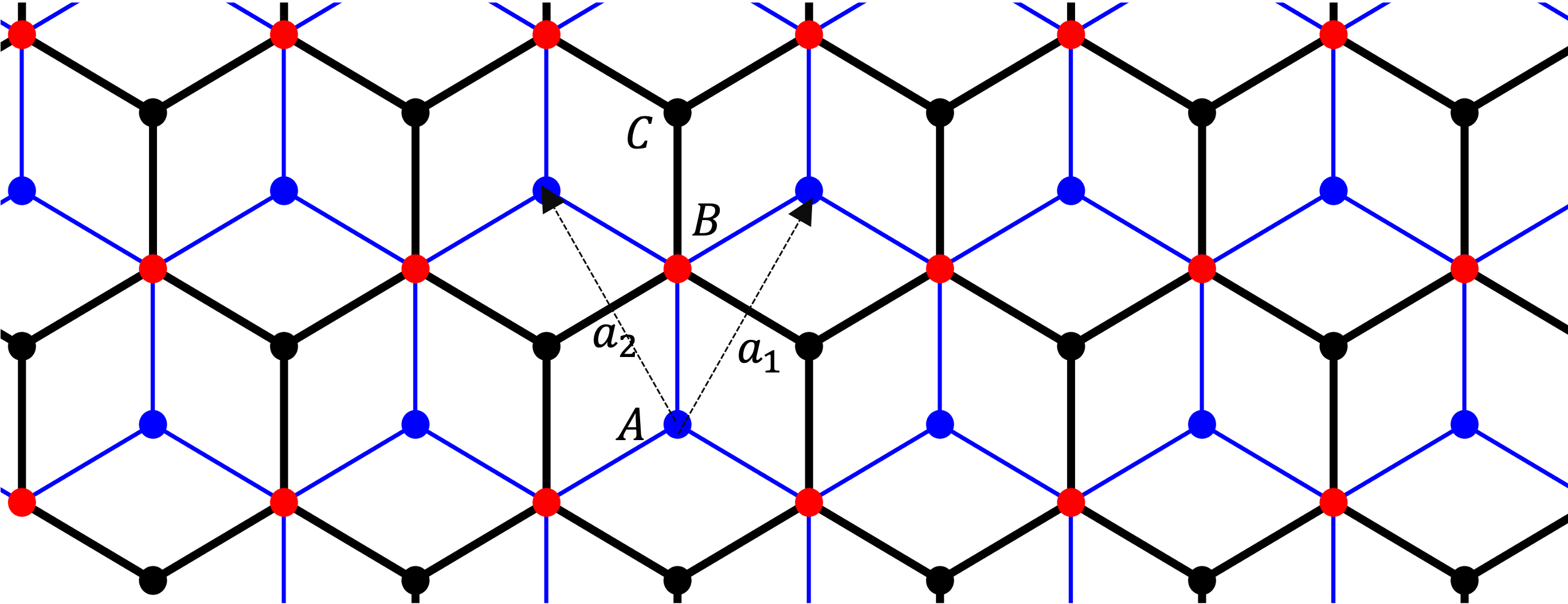
(a)

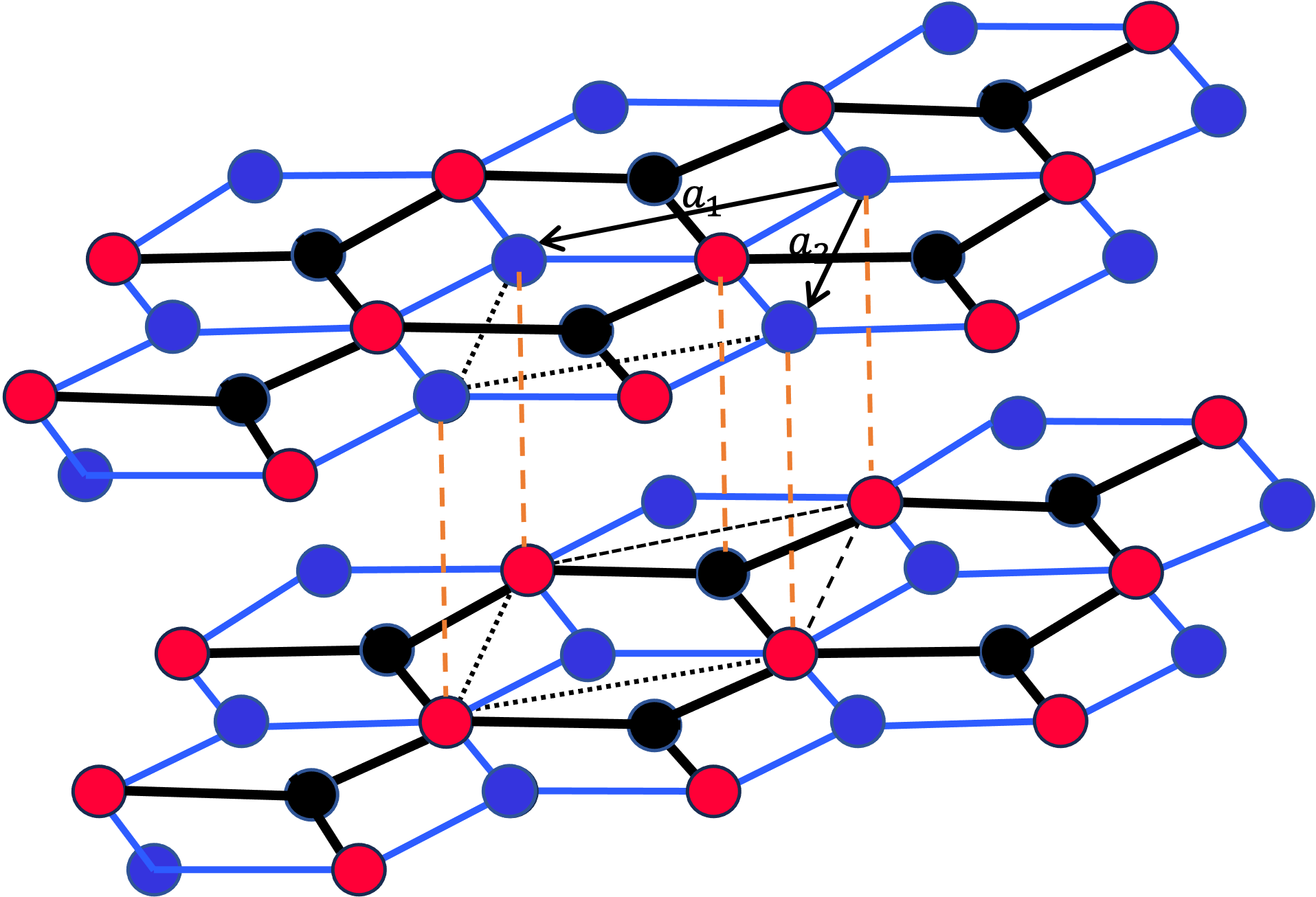
(b)

Figure 1: (color online) (a): Diagrams show the structure of dice lattice, blue dot indicate $A$ atoms, red dot $B$ indicate atoms and $C$ atoms for black dot. The lattice vectors described as $\bm{a_{1}}=a(\frac{1}{2},\frac{\sqrt{3}}{2}),\bm{a_{1}}=a(-\frac{1}{2},\frac{\sqrt{3}}{2})$, and corresponding reciprocal vectors $\bm{b_{1}}=\frac{4\pi}{\sqrt{3}a}(\frac{\sqrt{3}}{2},\frac{1}{2}),\bm{b_{2}}=\frac{4\pi}{\sqrt{3}a}(-\frac{\sqrt{3}}{2},\frac{1}{2})$, where $a=\sqrt{3}d$ is lattice constant. (b): Bilayer dice lattice in A-B stacking (Bernal). The hopping between A and C atoms in different layer are forbidden.

Since dice lattice can be realized in SrTiO3/SrIrO3/SrTiO3 trilayer heterostructure by growing along the (111) direction wang2011 , the TBD is possible to be realized in this material by twisting when growing.

For TBG, Bistritzer and MacDonald have proposed a low energy effective continuum Dirac model of the Moiré structure for small twist angle $\theta<10^{\degree}$. The effective model consists two isolated graphene layers and hopping terms between them. With this model they reveal flat Bloch bands in the electric structure at magic twist angles which give rise to large DOS Bistritzer-MacDonald2011 . Similar to the case of TBG, we follow Ref. Bistritzer-MacDonald2011 to constructed a continuum model for TBD. In TBD, we keep the top layer (Layer 1) fixed, and rotate the bottom layer (Layer 2) by $\theta$ with respect to Layer 1. The effective TBD Hamiltonian contains intralayer and interlayer parts. The low energy intra Hamiltonian reads

$$H=v_{f}\sum_{k}\psi_{1,\mathbf{k}}^{\dagger}\mathbf{S\cdot k}\psi_{1,\mathbf{k}}+v_{f}\sum_{k}\psi_{2,\mathbf{k}}^{\dagger}\mathbf{S_{\theta}\cdot k}\psi_{2,\mathbf{k}},$$ (A2)

where $S_{\theta}=e^{(i\theta/2)S_{3}}(S_{1},S_{2})e^{(-i\theta/2)S_{3}}$.

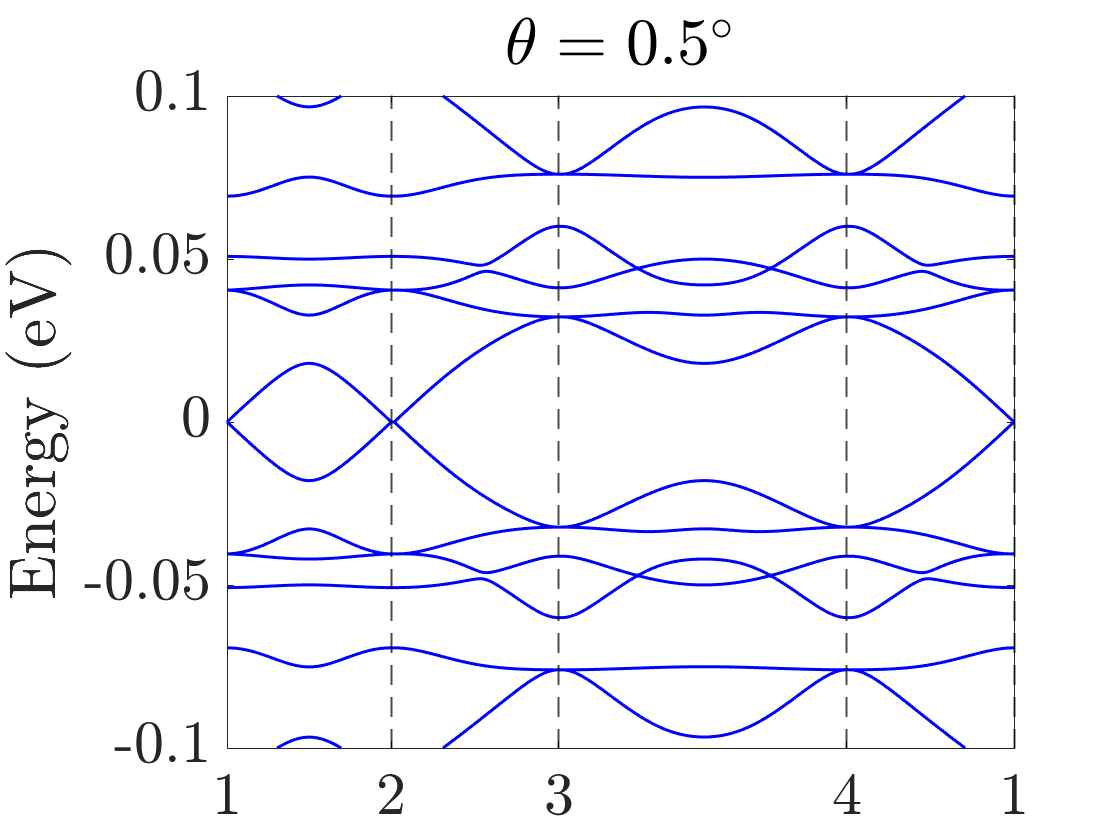
(a)

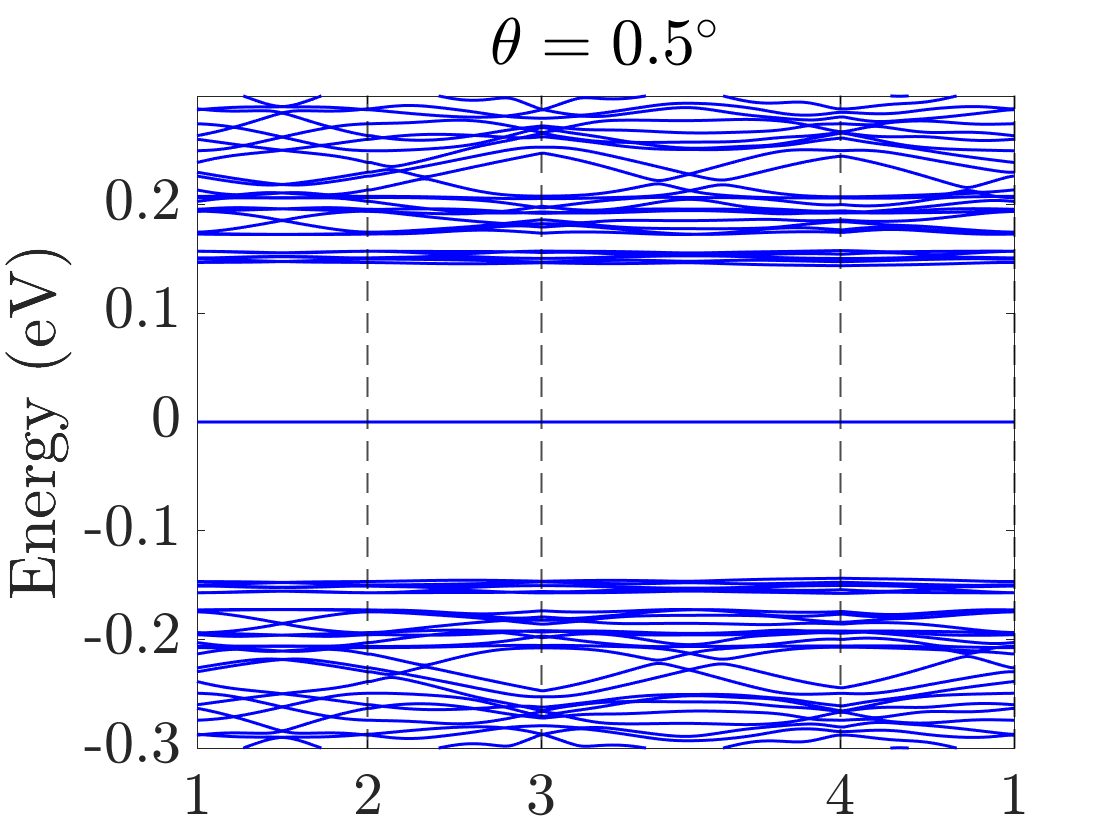
(b)

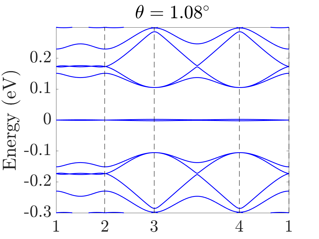
(c)

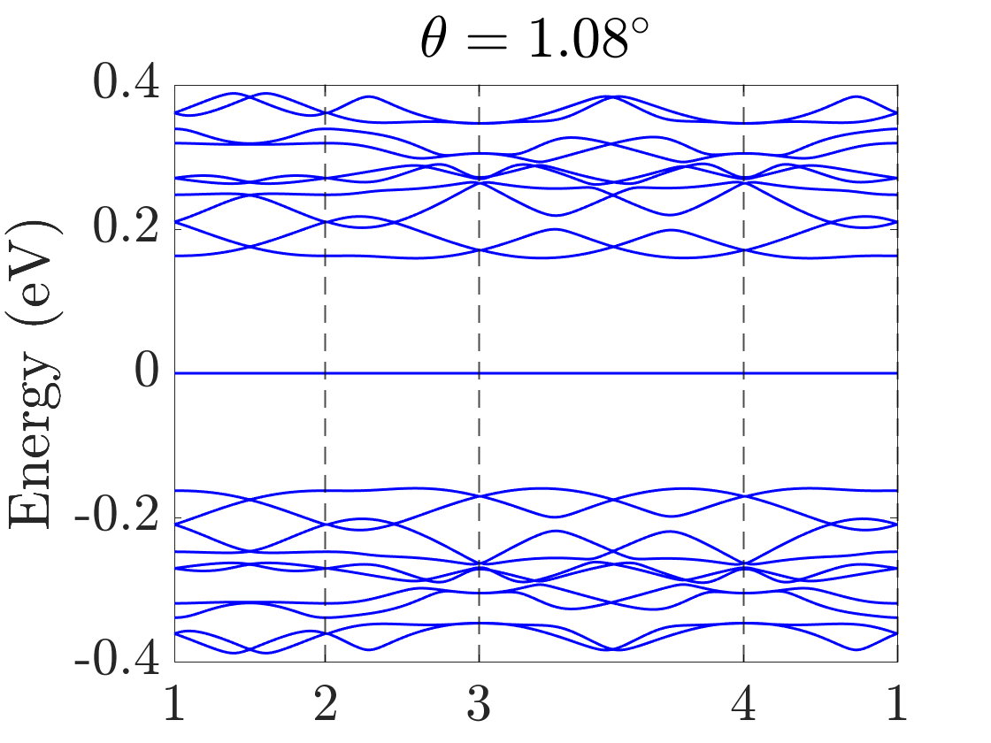
(d)

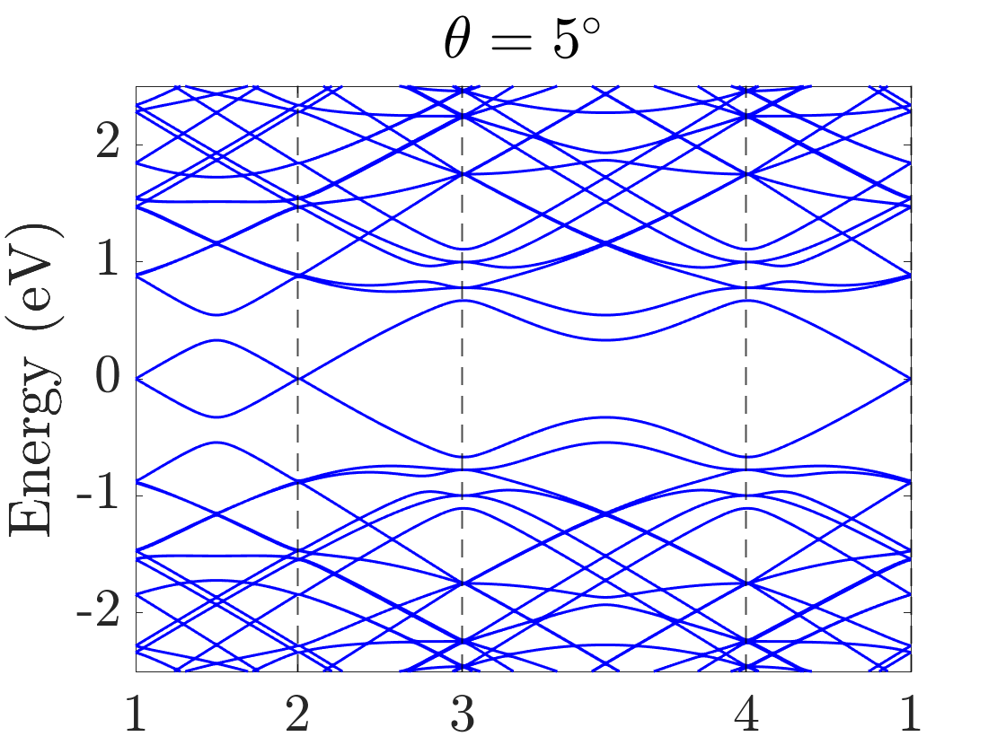
(e)

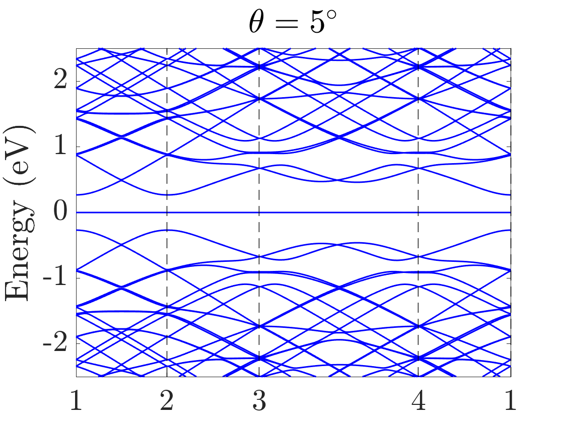
(f)

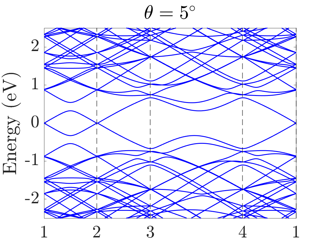
(g)

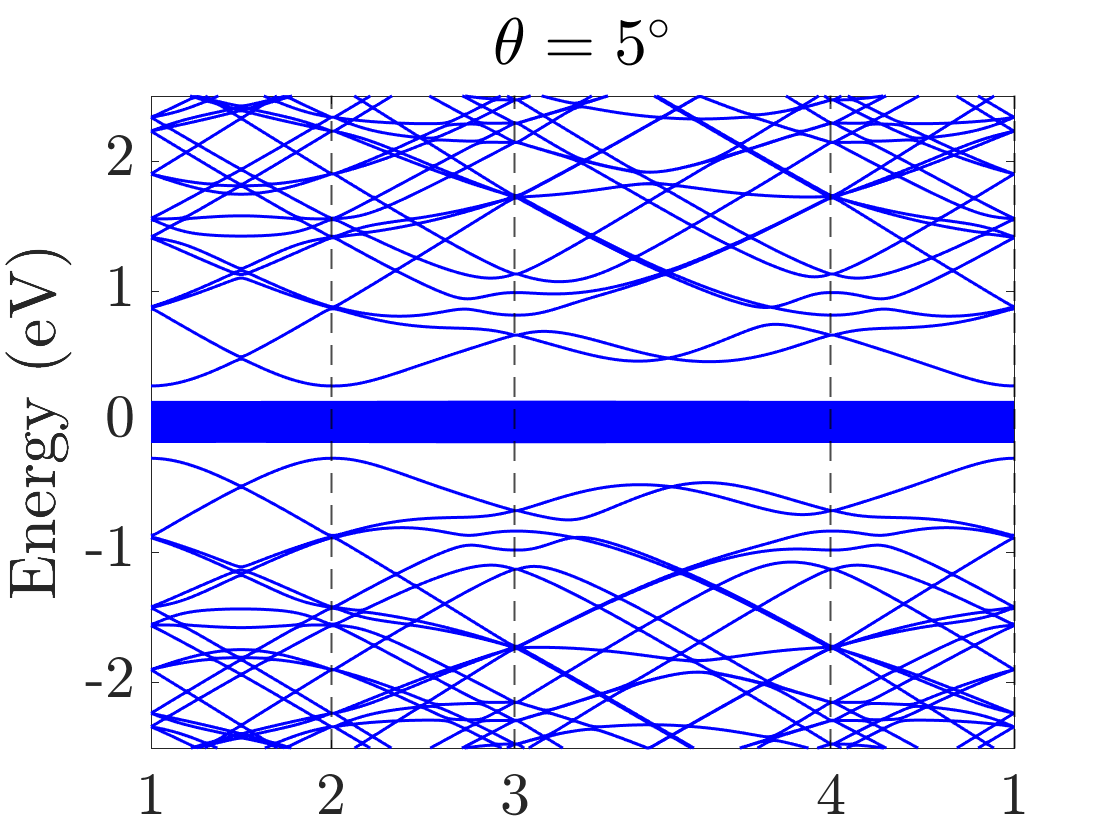
(h)

Figure 2: (color online) (a), (c), (e) The band structure of TBG lattices with hopping parameters $W_{AA^{\prime}}=0$ at twist angle $\theta=0.5^{\degree},1.08^{\degree},5^{\degree}$ respectively. The flat band only occurs at the magic angle $\theta=1.08^{\degree}$. (b), (d), (f) The band structure of TBD lattice as we set $W_{AA^{\prime}}=0$, totally flat band with high level degeneracy appears at zero energy at all angles. (g) and (h) are the band structures of TBG and TBD at twist angle $\theta=5^{\degree}$, $W_{AA^{\prime}}/W_{AB^{\prime}}=0.5$ respectively. In TBD, with the change of $W_{AA^{\prime}}$ from 0 to 1, the flat bands gradually spread. It is important to notice that we already set $W_{AC^{\prime}}=0$, which will break particl-hole symmetry at align bilayer dice lattice case. The momentum labels $1\rightarrow 2\rightarrow 3\rightarrow 4\rightarrow 1$ is defined in Fig. 3(b).

For the interlayer term $H_{\bot}$, we consider nearest neighbor hopping from layer 1 in $\alpha(\alpha=A,B,C)$ sublattice to closest sublattice $\beta(\beta=A^{\prime},B^{\prime},C^{\prime})$ in layer 2 (see Fig. 1).

$$H_{\bot}=\sum_{\mathbf{r}_{1},\mathbf{r}_{2},\alpha,\beta}c_{1,\alpha}^{\dagger}(\mathbf{r}_{1})t^{\alpha,\beta}_{1,2}(\mathbf{r}_{1},\mathbf{r}_{2})c_{2,\beta}(\mathbf{r}_{2})+h.c,$$ (A3)

where $t_{1,2}^{\alpha,\beta}=\bra{1,\mathbf{r}_{1},\alpha}H_{\bot}\ket{2,\mathbf{r}_{2},\beta}$. The band structure of aligned bilayer graphene is changed by the type of stacking, which is known as $AA$-stacked and $AB$-stacked (Bernal). For TBD, we set the aligned configuration coordinate as $\tau_{1,A}=\tau_{2,B^{\prime}}=(0,0),\tau_{1,B}=\tau_{2,C^{\prime}}=(0,d),\tau_{1,C}=\tau_{2,A^{\prime}}=(0,2d)$(see Fig. 1). To compare the results with TBG, we choose $1.42\text{\AA}$, the lattice constant of graphene.

The transition formula becomes

$$T^{\alpha,\beta}_{1,2}(\mathbf{k_{1}},\mathbf{k_{2}})=\frac{1}{A_{u.c}}\sum_{\mathbf{G}_{1},\mathbf{G}_{2}}e^{-i\mathbf{G}_{1}\cdot\tau_{1,\alpha}}t(K_{1}+\mathbf{q}_{1}+\mathbf{G}_{1})\cdot$$

$$e^{-i\mathbf{G}_{2}\cdot\tau_{1,\beta}}\delta_{K_{1}+\mathbf{q}_{1}+\mathbf{G}_{1},K_{2}+\mathbf{q}_{2}+\mathbf{G}_{2}}$$ (A4)

where $A_{u.c}$ is unit cell area, $K_{1,2}$ represent Dirac point for each layer which satisfy $K_{2}=R_{\theta}\cdot K_{1}$ where $R_{\theta}$ is the rotation matrix. Here we assume that interlayer hopping obeys $t^{\alpha,\beta}_{1,2}(\mathbf{r}_{1},\mathbf{r}_{2})=t^{\alpha,\beta}_{1,2}(\mathbf{r}_{1}+\tau_{1,\alpha}-\mathbf{r}_{2}-\tau_{2,\beta})$, which decays rapidly if $k$ in reciprocal space exceeds the Dirac pointBistritzer-MacDonald2011 . Considering this property we can only choose three vectors ${\bf 0}$, and $\mathbf{G}_{l}=\mathbf{g}_{l,1},\mathbf{g}_{l,2},\mathbf{g}_{l,3}$ with $\mathbf{g}_{l,1}=0,\mathbf{g}_{l,2}=\mathbf{b}_{l,2},\mathbf{g}_{l,3}=-\mathbf{b}_{l,1}$ being reciprocal lattice vectors and $l=1,2$ being layer index. Then we have three hopping matrices reads

$$T_{1}=W\begin{pmatrix}1&1&1\\ 1&1&1\\ 1&1&1\end{pmatrix},T_{2}=We^{-i\mathbf{g}_{1,2}\cdot\mathbf{\tau}_{0}}\begin{pmatrix}e^{i\phi}&1&e^{-i\phi}\\ e^{-i\phi}&e^{i\phi}&1\\ 1&e^{-i\phi}&e^{i\phi}\end{pmatrix},$$

$$T_{3}=We^{-i\mathbf{g}_{1,3}\cdot\mathbf{\tau}_{0}}\begin{pmatrix}e^{-i\phi}&1&e^{i\phi}\\ e^{i\phi}&e^{-i\phi}&1\\ 1&e^{i\phi}&e^{-i\phi}\end{pmatrix},$$ (A5)

where $W=\frac{t(|K|)}{A_{u.c}}=110meV$ with $|K|=4\pi/(3\sqrt{3}d)$ as in graphene Bistritzer-MacDonald2011 , and $\phi=2\pi/3$.

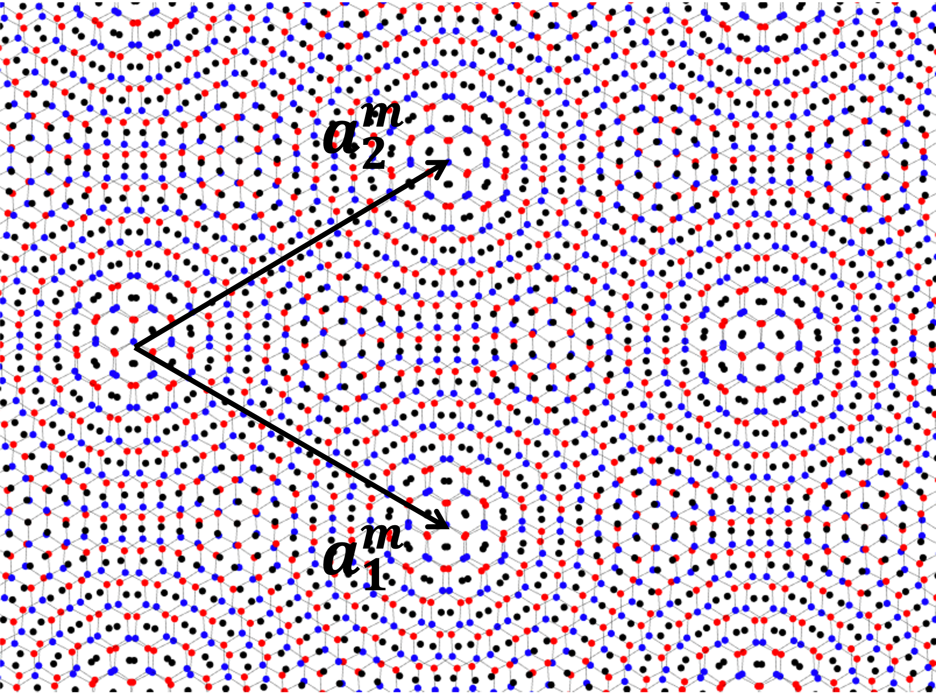
(a)

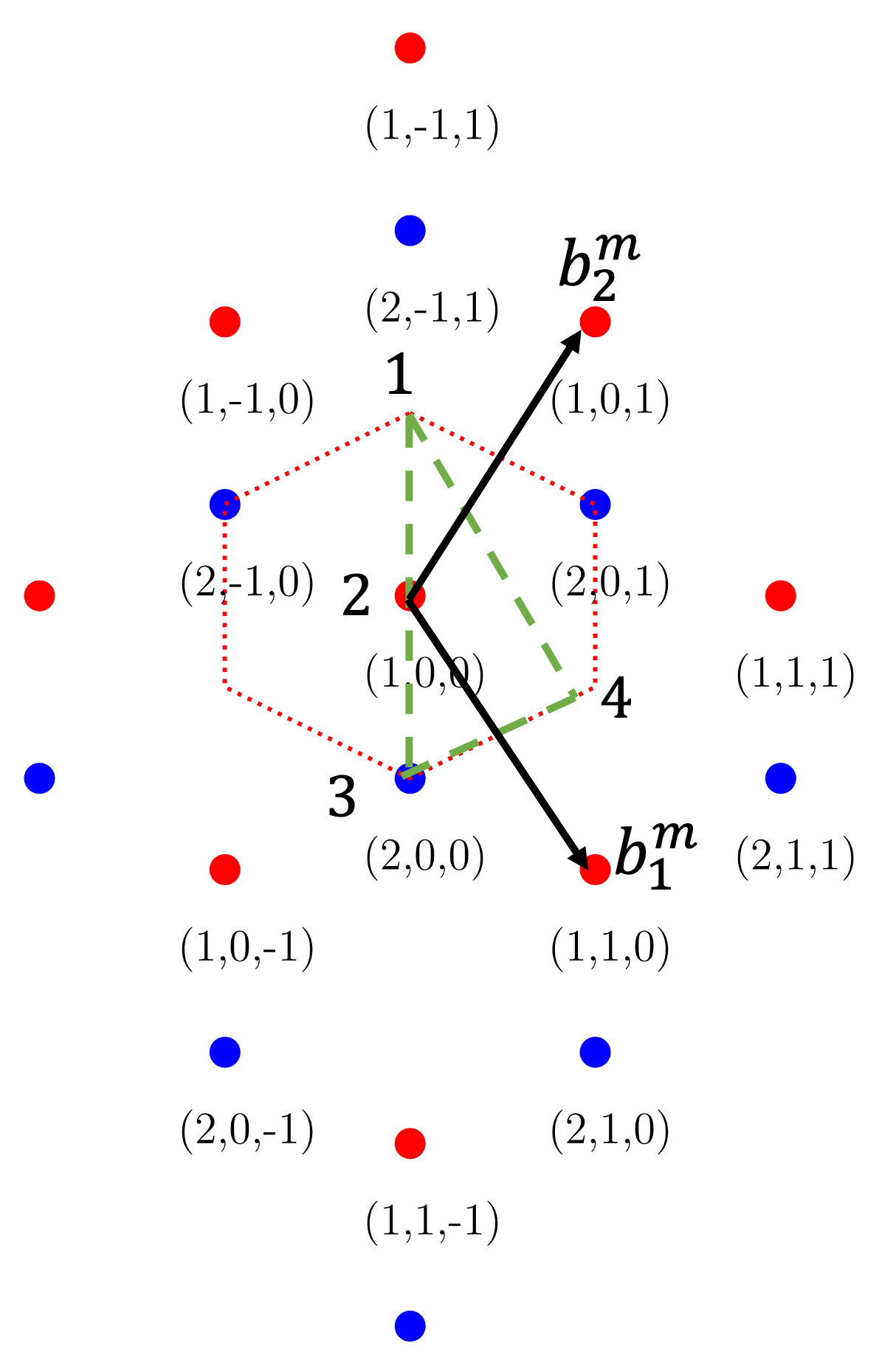
(b)

Figure 3: (color online) (a): The Moiré period structure of dice lattice which unit cell described by its Moiré lattice vectors reads $\bm{a_{1}^{m}}=L_{s}(\frac{\sqrt{3}}{2},-\frac{1}{2}),\bm{a_{2}^{m}}=L_{s}(\frac{\sqrt{3}}{2},\frac{1}{2})$, where $L_{s}=\frac{a}{2\sin(\theta/2)}$ is size of Moiré unit cell. (b): Reciprocal space of TBD with reciprocal vectors reads $\bm{b^{m}_{1}}=\frac{4\pi}{\sqrt{3}L_{s}}(\frac{1}{2},-\frac{\sqrt{3}}{2}),\bm{b^{m}_{2}}=\frac{4\pi}{\sqrt{3}L_{s}}(\frac{1}{2},\frac{\sqrt{3}}{2})$, and red dash line mark the first Brillouin zone with green dash line mark the reciprocal path of TBD band structure. We use Bravais lattice vectors mapping the reciprocal space of TBD like $\bm{b}=l_{1}\bm{b^{m}_{1}}+l_{2}\bm{b^{m}_{2}}$, the first number represent the layer index which also represent by red point(layer 1) and blue point(layer2).

III Comparing the band structures of TBG and TBD

After building effective model of TBD, we now can compare the band structures of TBG and TBD. In our previous calculation, we assume the hopping term is isotropic, namely, the hopping amplitude of different sublattice equal to each other, which induces $W_{AA^{\prime}}=W_{AB^{\prime}}$. In TBG, the absolutely flat band at magic angle $\theta\approx 1.08^{\degree}$ can be obtained in the chiral limit, namely, by choosing $W_{AA^{\prime}}=0$ Tarnopolsky2019 . In the chiral limit of TBD, highly degenerate flat bands at zero energy also exist. In our model, the chiral limit corresponds to setting $W_{AA^{\prime}}=W_{AC^{\prime}}=0$. $W_{AC^{\prime}}$ is a new ingredient in TBD when comparing with TBG, and the effects of non-zero $W_{AC^{\prime}}$ will be discussed at the end of this section. We set parameter $W=110mev$, and truncate Hamiltonian at order of $l_{1}=l_{2}=3$, meanwhile we choose three moiré angle $\theta=0.5^{\degree},1.08^{\degree},5^{\degree}$, and final results of the band structure are summarized in Fig.2.

Unlike TBG which has flat bands near magic angles, TBD has flat bands at all angles, which is the manifestation of flat band of single layer dice lattice model (see Fig. 2). These TBD flat bands are highly degenerate in the chiral limit. When $W_{AA^{\prime}}$ and $W_{AC^{\prime}}$ are nonzero, the degeneracy is lifted and behaves as Landau levels (see Fig. 5b).

When $W_{AA^{\prime}}$ is non-zero, the degeneracy of the central flat bands is lifted. As $W_{AA^{\prime}}$ increases, we can observe from Fig. 2h that the range of the central flat band gradually expands, where we have set $W_{AC^{\prime}}=0$. Interestingly, in the TBD system, even if we set the parameter $W_{AA^{\prime}}$ = 0, changing the value of $W_{AC^{\prime}}$ can also lead to the lifting of degeneracy in $\theta=0.5^{\degree},1.08^{\degree},5^{\degree}$. Therefore, to obtain the band structure of the central flat band, both parameters, $W_{AA^{\prime}}$ and $W_{AC^{\prime}}$, must be set to zero. Additionally, when the two layers are aligned, the parameter $W_{AC^{\prime}}$ affects particle-hole symmetry. Meanwhile, in TBD under the condition both $W_{AA^{\prime}}\neq 0$ and $W_{AC^{\prime}}\neq 0$, the particle-hole symmetry will also be broken.

After discussing the effects of parameters $W_{AA^{\prime}}$ and $W_{AC^{\prime}}$ on the flat band structure of TBD system, we now turn to their effects on the band structure in align bilayer case. In both perfect aligned stacking and A-B stacking bilayer dice lattice, the parameter $W_{AC^{\prime}}$ will significantly affect the particle-hole symmetry of the band. First we have the Hamiltonian of A-B align bilayer dice lattice reads

$$H=\begin{pmatrix}0&h(\bm{k})&0&0&t_{\bot}&0\\ h^{*}(\bm{k})&0&f(\bm{k})&0&0&t_{\bot}\\ 0&f^{*}(\bm{k})&0&0&0&0\\ 0&0&0&0&h(\bm{k})&0\\ t_{\bot}&0&0&h^{*}(\bm{k})&0&f(\bm{k})\\ 0&t_{\bot}&0&0&f^{*}(\bm{k})&0\end{pmatrix},$$ (A6)

where $h(\bm{k})=-\tau(e^{i\bm{k}\cdot\tau_{B}}+e^{i\bm{k}\cdot(\tau_{B}-a_{1})}+e^{i\bm{k}\cdot(\tau_{B}-a_{2})})$, and corresponding $f(k)=-\tau(e^{i\bm{k}\cdot(\tau_{B}-\tau_{C})}+e^{i\bm{k}\cdot(\tau_{B}-a_{1}-\tau_{C})}+e^{i\bm{k}\cdot(\tau_{B}-a_{2}-\tau_{C})})$ which $\tau=\sqrt{2}v_{f}\hbar/(3d)$. The hopping amplitude of A-B sublattice same with graphene and the basis of bilayer align dice lattices is $\Psi^{\dagger}=[c^{\dagger}_{1,A},c^{\dagger}_{1,B},c^{\dagger}_{1,C},c^{\dagger}_{2,A^{\prime}},c^{\dagger}_{2,B^{\prime}},c^{\dagger}_{2,C^{\prime}}]$. The position of atoms B and C in one unit cell are $\tau_{B}=d(0,1),\tau_{C}=d(0,2)$, and $d$ is lattice constant. It is worth noticing that we set hopping parameter $W_{AC^{\prime}}=0$ in order to maintain particle-hole symmetry of system. The band structure of two different ways of stacking shown in Fig.4

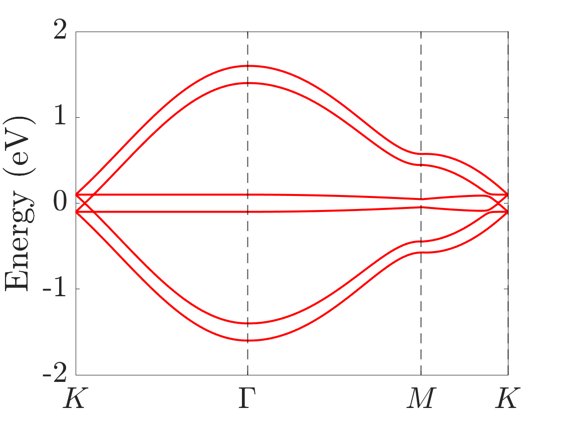
(a)

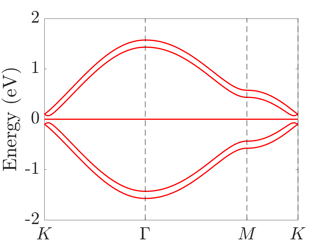
(b)

Figure 4: (color online) Here we set reciprocal path same with graphenecatarina2019twisted , lattices vector and coordinate of atoms in unit cell same with Fig.1. (a) The band structure of A-A stacking(perfect align), here we set hopping amplitude $t_{A,A^{\prime}}=t_{B,B^{\prime}}=t_{C,C^{\prime}}=0.33eV$. (b) The band structure of A-B stacking(Bernal-stack), in this case hopping between $A$ and $C^{\prime}$ sublattices is forbidden because of particle-hole symmetry, $t_{A,B^{\prime}}=t_{B,C^{\prime}}=0.33eV$2016PhR…648….1R .

IV $SU(2)$ symmetry and Landau level structure

We have assumed chiral limit in the previous calculations of the band structure, while in real TBG system at small twist angle $\theta\leq 10^{\degree}$, the lattice period will be dependent on different atomic stacking and cause atomic layer deformation PhysRevB.90.155451 , which eventually drives the system away from the chiral limit. This effect can be described by introducing interlayer couplings which can be represented by an $SU(2)$ gauge potential Liu2019Pseudo ; San-Jose2012Non-Abelian ; ren2021 . Similar to TBG, one can write the low energy Hamiltonian as

$$H=-\hbar v_{f}(\mathbf{k}-\frac{e}{\hbar}\mathbf{A}\tau_{2})\cdot S+3u_{0}\tau_{1},$$ (A7)

where $3u_{0}$ represents the hopping parameter $W_{AA^{\prime}}$ which transforms into a scalar potential Liu2019Pseudo , and $\tau_{1,2}$ are the Pauli matrices that act on the layer index. The gauge potential reads $\mathbf{A}=(2\pi u^{\prime}_{0})/(L_{s}ev_{f})(y,-x)$, $u^{\prime}_{0}$ denote hopping parameters $W_{AB^{\prime}},W_{BC^{\prime}}$ in our system and $u_{0}$ denote $W_{AA^{\prime}}$. The effective magnetic field ${\bf B}=\nabla\times{\bf A}\approx 120T$ for TBG at $\theta\approx 1.08^{\degree}$ Liu2019Pseudo . The effective magnetic field has opposite directions on each layer, therefore time-reversal symmetry is preserved. In the following numerical calculations, we set $u^{\prime}_{0}=0.01eV,u_{0}=0.1eV$. A comparison between the effective continuous Hamiltonian and the Landau level description is presented in Appendix A, which also supports the usage of the Landau level method.

To discuss the Landau level structure, we transform the Hamiltonian (A7) into basis of $\tau_{2}$

$${\scriptsize H(\mathbf{k})=\begin{pmatrix}0&\pi_{x}+i\pi_{y}&0&3iu_{0}&0&0\\ \pi_{x}-i\pi_{y}&0&\pi_{x}+i\pi_{y}&0&3iu_{0}&0\\ 0&\pi_{x}-i\pi_{y}&0&0&0&3iu_{0}\\ -3iu_{0}&0&0&0&\pi^{\prime}_{x}+i\pi^{\prime}_{y}&0\\ 0&-3iu_{0}&0&\pi^{\prime}_{x}-i\pi^{\prime}_{y}&0&\pi^{\prime}_{x}+i\pi^{\prime}_{y}\\ 0&0&-3iu_{0}&0&\pi^{\prime}_{x}-i\pi^{\prime}_{y}&0\end{pmatrix}},$$ (A8)

where $\pi_{x}=\hbar v_{f}k_{x}-ev_{f}A_{x}$, $\pi_{y}=-\hbar v_{f}k_{y}+ev_{f}A_{y}$, $\pi^{\prime}_{x}=\hbar v_{f}k_{x}+ev_{f}A_{x}$, and $\pi^{\prime}_{y}=-\hbar v_{f}k_{y}-ev_{f}A_{y}$. Since $u_{0}$ is small, we can treat it as a perturbation. Then for the unperturbed Hamiltonian $H_{0}$, we define the Landau level creation operators of the two layers, $b^{\dagger}=\sqrt{\frac{L_{s}}{8\pi u^{\prime}_{0}\hbar v_{f}}}(\pi_{x}-i\pi_{y})$, and $a^{\dagger}=\sqrt{\frac{L_{s}}{8\pi u^{\prime}_{0}\hbar v_{f}}}(\pi^{\prime}_{x}+i\pi^{\prime}_{y})$. And the nonzero commutators are $[b,b^{\dagger}]=[a,a^{\dagger}]=1$. Denoting the unperturbed eigenfunction as $\ket{\Psi}$,

$$H_{0}(\mathbf{k})\ket{\Psi}=\hbar w\begin{pmatrix}0&b&0&0&0&0\\ b^{\dagger}&0&b&0&0&0\\ 0&b^{\dagger}&0&0&0&0\\ 0&0&0&0&a^{\dagger}&0\\ 0&0&0&a&0&a^{\dagger}\\ 0&0&0&0&a&0\end{pmatrix}\begin{pmatrix}A^{1}_{n}\ket{n-1}\\ A^{2}_{n}\ket{n}\\ A^{3}_{n}\ket{n+1}\\ B^{1}_{m}\ket{m+1}\\ B^{2}_{m}\ket{m}\\ B^{3}_{m}\ket{m-1}\end{pmatrix},$$ (A9)

where $\hbar w=\sqrt{\frac{8\pi u^{\prime}_{0}\hbar v_{f}}{L_{s}}}$, $\ket{n},\ket{m}$ denote Landau levels with $b\ket{n}=\sqrt{n}\ket{n-1},b^{\dagger}\ket{n}=\sqrt{n+1}\ket{n+1},a^{\dagger}\ket{m}=\sqrt{m+1}\ket{m+1},a\ket{m}=\sqrt{m}\ket{m-1}$.

The spectra of $H_{0}(\mathbf{k})$ For $n,m>0$ reads

$$E_{\pm}^{n,m}=\pm\hbar w\sqrt{2(n,m)+1},\quad E_{0}^{n,m}=0.$$ (A10)

Due to the quasi spin-1 nature of the sublattice structure of Dice model, For $n,m=0$,

$$E^{0}_{\pm}=\pm\hbar w,$$ (A11)

Which correspond to the 1st Landau levels in the upper and lower layers. And the $E=0$ for the 0th Landau level with $n,m=-1$. As mentioned before, $n(m)$ labels the states in Layer 1(2), therefore we use $1(2)$ to denote the corresponding wave functions.

The wavefunctions for $m,n=1,2,3...$ are

$$\ket{\Psi}^{1}_{\pm}=\begin{pmatrix}\sqrt{\frac{n}{4n+2}}\ket{n-1}\\ \pm\sqrt{\frac{2n+1}{4n+2}}\ket{n}\\ \sqrt{\frac{n+1}{4n+2}}\ket{n+1}\\ 0\\ 0\\ 0\end{pmatrix},\ket{\Psi}^{2}_{\pm}=\begin{pmatrix}0\\ 0\\ 0\\ \sqrt{\frac{m+1}{4m+2}}\ket{m+1}\\ \pm\sqrt{\frac{2m+1}{4m+2}}\ket{m}\\ \sqrt{\frac{m}{4m+2}}\ket{m-1}\\ \end{pmatrix},$$ (A12)

$$\ket{\Psi}^{1}_{0}=\begin{pmatrix}-\sqrt{\frac{n+1}{2n+1}}\ket{n-1}\\ 0\ket{n}\\ \sqrt{\frac{n}{2n+1}}\ket{n+1}\\ 0\\ 0\\ 0\end{pmatrix},\ket{\Psi}^{2}_{0}=\begin{pmatrix}0\\ 0\\ 0\\ -\sqrt{\frac{m}{2m+1}}\ket{m+1}\\ 0\ket{m}\\ \sqrt{\frac{m+1}{2m+1}}\ket{m-1}\\ \end{pmatrix}.$$ (A13)

For $n,m=0$, we have

$$\ket{\Psi}^{1}_{\pm}=\sqrt{\frac{1}{2}}\begin{pmatrix}0\\ \pm\ket{0}\\ \ket{1}\\ 0\\ 0\\ 0\end{pmatrix},\quad\ket{\Psi}^{2}_{\pm}=\sqrt{\frac{1}{2}}\begin{pmatrix}0\\ 0\\ 0\\ \ket{1}\\ \pm\ket{0}\\ 0\end{pmatrix},$$ (A14)

and for $n,m=-1$

$$\ket{\Psi}^{1}_{0}=\begin{pmatrix}0\\ 0\\ \ket{0}\\ 0\\ 0\\ 0\end{pmatrix},\quad\ket{\Psi}^{2}_{0}=\begin{pmatrix}0\\ 0\\ 0\\ \ket{0}\\ 0\\ 0\end{pmatrix}.$$ (A15)

The band structure is illustrated in Fig.5, which is similar to the band structure in Fig. 2. And the lifting of the degeneracy of flat bands is caused by the perturbation $u_{0}$, the interlayer hopping. After perturbation, a double degeneracy remains which is related to the $S_{3}$ symmetry (the pseudo-spin in the $z$ direction) Liu2019Pseudo .

V Optical conductance

In reality, materials that rotates the polarization plane of linearly polarized light have lots of applications in various devices, which is usually achieved by the magneto-optical effects, quantum Hall effect, and the Kerr and Faraday rotations by invoking external magnetic fields oc1 ; oc2 ; oc3 ; oc4 ; oc5 ; oc6 ; oc7 , which also limits the applications in small-scale devices. Therefore, searching for materials with intrinsic properties that rotates light is urgent for recent applications. The TBG is such a candidate for advanced optical applications due to the tunable twist angles occ1 ; occ2 . Here we study the optical conductance of TBD, which could be another candidate for such applications.

We utilize Kubo formula in Landau level basis to calculate the optical conductance of TBD system PhysRevB.94.125435 ,

$$\sigma_{\alpha,\beta}=\frac{ig}{2\pi\hbar l^{2}_{B}}\sum_{LL_{s}}\frac{f-f^{\prime}}{\varepsilon^{\prime}-\varepsilon}\frac{\braket{\Psi}{j_{\alpha}}{\Psi^{\prime}}\braket{\Psi^{\prime}}{j_{\beta}}{\Psi}}{w-(\varepsilon^{\prime}-\varepsilon)+i\Gamma},$$ (A16)

where $l_{B}=\sqrt{(L_{s}hcv_{f})/4\pi u^{\prime}_{0}}$ is magnetic length, without considering spin degree of freedom we can simply set $g=2$, $f$ is Fermi distribution meanwhile $w$ is photon energy. Here we shall emphasize that, although we use the Landau level description, no magnetic field is applied. The effective magnetic field is induced by the hopping of $W_{AB^{\prime}}$ and $W_{BC^{\prime}}$, and the effective magnetic field has opposite directions on top and bottom layers of TBD. Therefore time-reversal symmetry is preserved.

We take into account the contribution of all Landau levels, however the remaining double degeneracy of the band structure will cause divergence of conductance. For doubly-degenerate band, we fix the divergent part of Kubo formula (A16) into

$$\lim_{\epsilon^{\prime}-\epsilon\to 0}\frac{f(\epsilon)-f^{\prime}(\epsilon^{\prime})}{\epsilon^{\prime}-\epsilon}=\frac{e^{(\epsilon_{0}-\mu)/kT}}{(e^{(\epsilon_{0}-\mu)/kT}+1)^{2}}\cdot\frac{1}{kT}.$$ (A17)

From Hamiltonian (A8), the current is obtained by $j_{\alpha,\beta}=\frac{\delta H_{0}(\mathbf{k})}{\delta A_{\alpha,\beta}}$,

$$j_{x}=ev_{f}\begin{pmatrix}0&-1&0&0&0&0\\ -1&0&-1&0&0&0\\ 0&-1&0&0&0&0\\ 0&0&0&0&1&0\\ \ 0&0&0&1&0&1\\ 0&0&0&0&1&0\end{pmatrix},$$ (A18)

$$j_{y}=ev_{f}\begin{pmatrix}0&i&0&0&0&0\\ -i&0&i&0&0&0\\ 0&-i&0&0&0&0\\ 0&0&0&0&-i&0\\ \ 0&0&0&i&0&-i\\ 0&0&0&0&i&0\end{pmatrix}.$$ (A19)

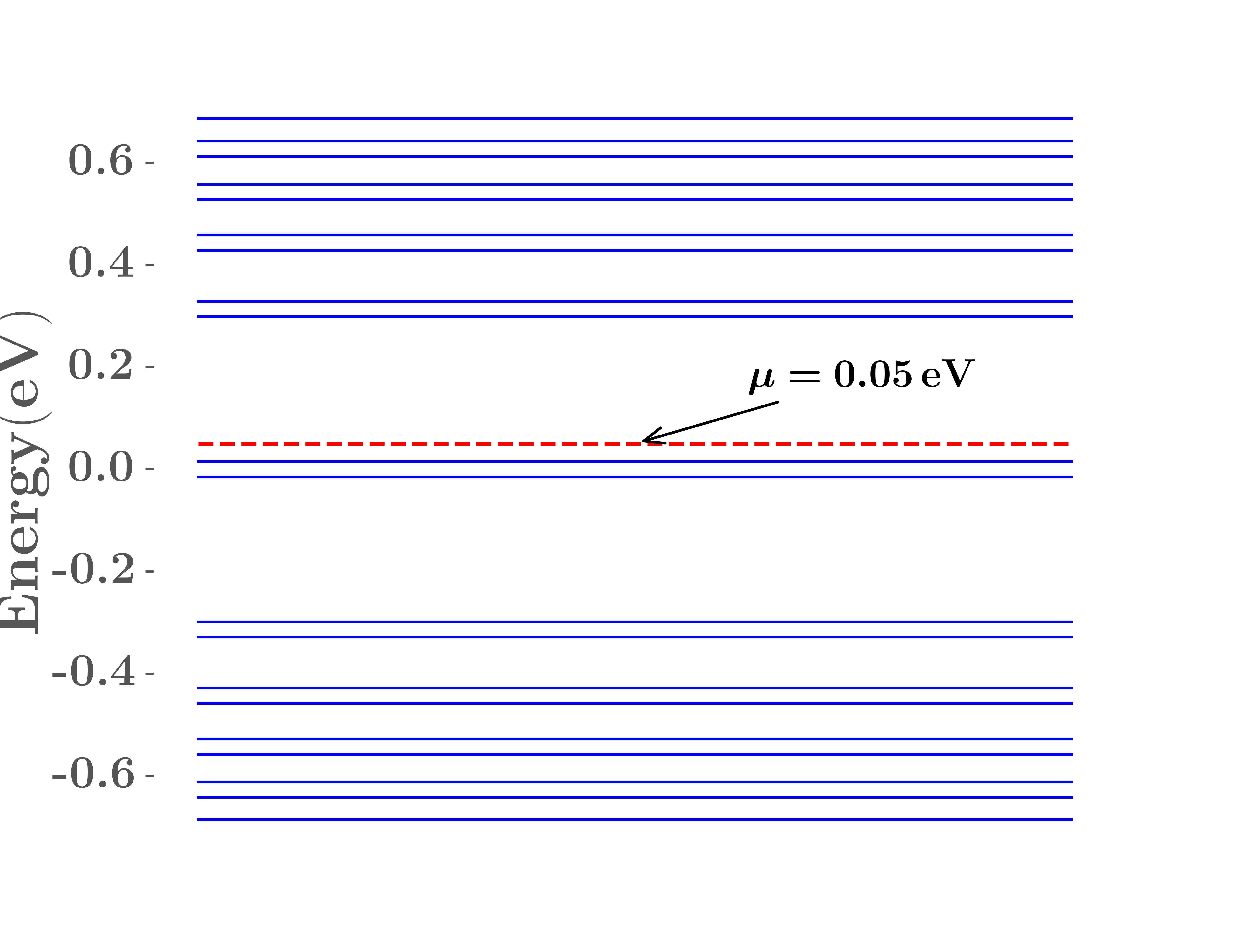
(a)

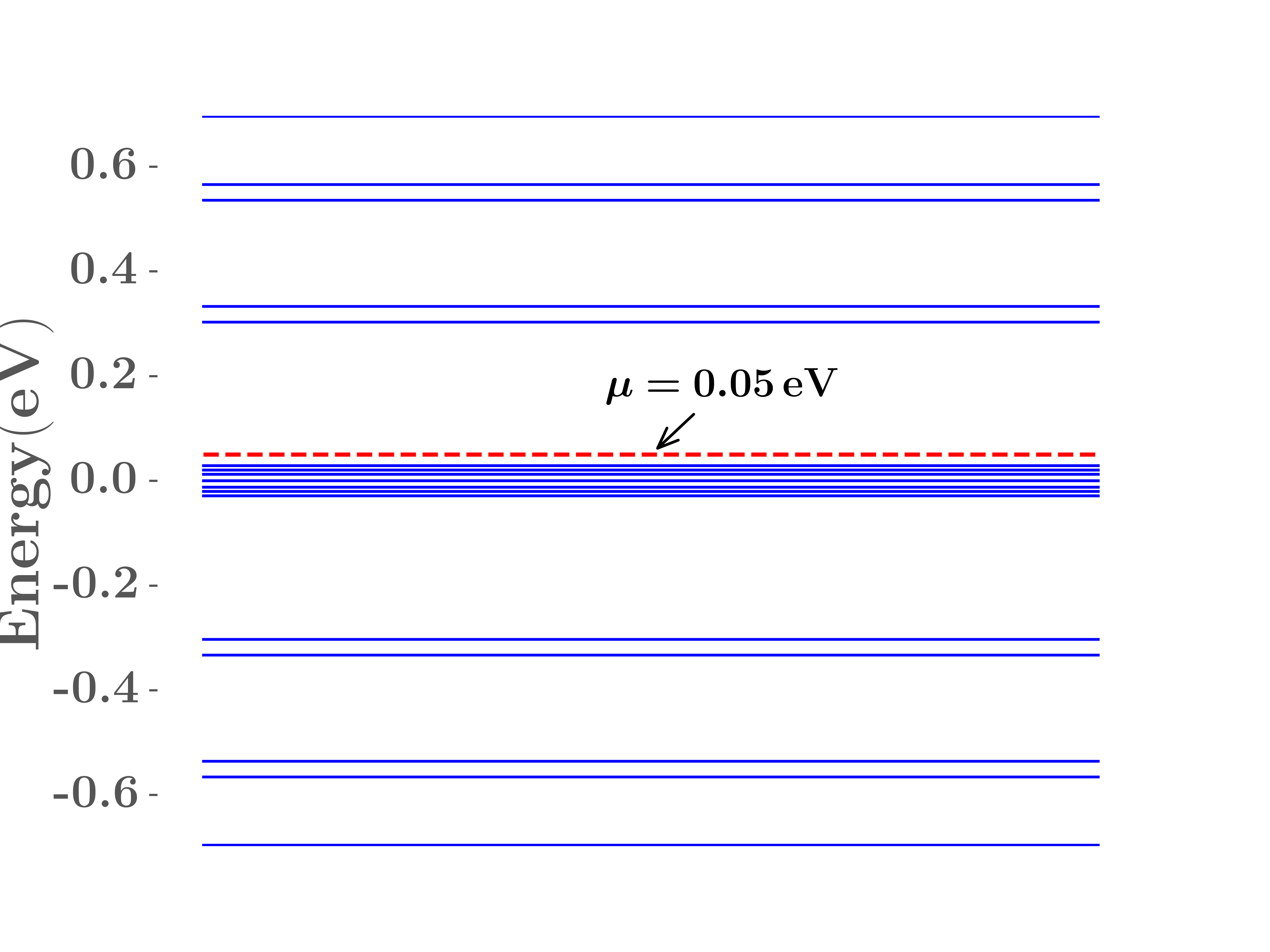
(b)

(c)

(d)

Figure 5: (color online) (a) The Landau level of TBG lattice in the vicinity of $K_{1}$ and $K_{2}$ with chemical potential $\mu=0.05eV$ (the red dotted line). (b) The Landau level of TBD with same chemical potential of TBD. (c) Optical conductance of TBG with same truncation, $\pm$ represent the two flat band near zero energy, for the band bigger(smaller) we denote as $L=0^{\pm},\pm 1,\pm 2,...$. For example, $T_{\pm,0^{+}}$ represents the contribution from two flat bands to first upper branch Landau level denoted by $L=0^{+}$. (d) Optical conductance of TBD with truncate $n=m=6$, we denote the Landau levels(without flat band near zero energy) with integer $L=0^{\pm},\pm 1,\pm 2,...$, $0^{+}$ denoting upper branch and $0^{-}$ lower branch. For flat band we use their energy value to denote, for example $T_{-0.012,0^{+}}$ respects contribution from flat band with energy $E=-0.012eV$ to first upper branch Landau level denoted by $L=0^{+}$.

The numerical result for $\mu=0.05eV$ and $T=300K$ of the conductance of TBD lattice is shown in Fig. 5(c). The double peak structure is caused by the splitting of double degeneracy, and the width of splitting depends on $u^{\prime}_{0}$. Due to the choice of chemical potential, Meanwhile, because of the high DOS in the near zero band of Landau level, all significant absorption peaks are originated from transitions between the near zero band and the positive energy band, or between the bottom valence band and the near zero band. By comparing with the result of TBG in Fig. 5(d), the fine structure of TBD provides a smoking-gun experiment prediction for showing the existence of these near zero energy bands.

Although the Landau level description for TBG fails when the twist angle is away from the magic ones, the Landau level structure remains in TBD (see Figs. 2g and 2h). Therefore in the optical conductance at angles other than the magic ones, the peak splitting remains in TBD while the peaks raising from the transitions form the flat bands disappear in TBG, which is also a key experimental difference between TBG and TBD.

The transitions between these zero energy levels are forbidden in TBD, which meanings that there are no peaks at low frequency near $\omega\sim 0$, which is a key difference to the three-dimensional Kane fermion Luo2019 . The reason of this phenomenon attributed to the structure of current and wavefunction in 2D, that is, $\braket{\Psi}{j_{\alpha}}{\Psi^{\prime}}\braket{\Psi^{\prime}}{j_{\beta}}{\Psi}=0$ between those near zero band, and their contribution to the optical conductance is zero, while in three-dimensional, the $k_{3}S_{3}$ part will have a nontrivial contribution, and the transition between different Landau levels has a non zero $k_{3}$, which causes the peaks near zero frequency Luo2019 .

VI Conclusions

In this paper, we constructed a lattice model for TBD. It has flat bands at all twisted angles besides the magic ones, which could be conformed by the peak splitting fine structure of the optical conductance near the magic angles. And away from the magic angles, the peak splitting remains in TBD while these peaks disappear in TBG due to the nonexistence of the flat bands. The flat bands in TBD are composed of zero Chern number ones by destructive interference of the dice lattice as well as the topological nontrivial ones by the Moiré structure at the magic angles. In this model we have neglected the spin degrees of freedom of electrons. If the spin orbital coupling interaction is added, the bands with zero Chern number may become non-trivial wang2011 . The TBD is possible to be realized in the transition-metal oxide SrTiO3/SrIrO3/SrTiO3 trilayer heterostructure by growing and twisting along the (111) direction. As a semiconductor, due to the large DOS of the flat bands of TBD, it may have potential applications on temperature-sensitive, photosensitive manipulations. With interactions, TBD may also be a good candidate for fractional Chern insulator.

Appendix A Density of states of two different system

In our previous discussions, we follow Ref. Bistritzer-MacDonald2011 to construct a tight-binding model for TBG and TBD lattice in reciprocal space. To discuss the influence of parameters $W_{AC^{\prime}}$ and $W_{AA^{\prime}}$ on the spectrum of these models, we also consider the chiral limitLiu2019Pseudo ; San-Jose2012Non-Abelian for a comparison. In order to compute the optical conductance of both models, we use the pseudo-Landau level description (A7) of the effective theory. In order to verify applicability of the Landau level scenario, we construct a reciprocal space tight-binding model in Landau basis, and compare the density of states (DOS) between this model and the one generated from Ref. Bistritzer-MacDonald2011 . We find that they have similar behaviors (see Fig. 6), especially, they have a high DOS at the zero energy near the magic angle of $1.08^{\degree}$, which supports the usage of the effective description of pseudo-Landau levels.

The low energy Dirac equation reads

$$H=-\hbar v_{f}(\mathbf{k}-\frac{e}{\hbar}\mathbf{A}\tau_{2})\cdot\bm{\sigma}+3u_{0}\tau_{1},$$ (A1)

where hopping matrices reads

$$T=\begin{pmatrix}\psi_{1,A}^{\dagger}&\psi_{1,B}^{\dagger}\end{pmatrix}\begin{pmatrix}3iu_{0}&0\\ 0&3iu_{0}\\ \end{pmatrix}\begin{pmatrix}\psi_{2,A^{\prime}}\\ \psi_{2,B^{\prime}}\end{pmatrix},$$ (A2)

(a)

(b)

Figure 6: (color online) (a) DOS of TBG mode which calculated using Landau level model with $\theta=1.08^{\degree}$ and $u_{0}/u_{0}^{\prime}=0.2$. (b) DOS of TBG is calculated by using continuum model with $W_{AA^{\prime}}=W_{AB^{\prime}}$ and $\theta=1.08^{\degree}$. We calculate this result in order to compare with Ref. Bistritzer-MacDonald2011 . For more details see Appendix A.

after transforming into the Landau basis, the Hamiltonian of intralayer reads

$$H_{0}(\mathbf{k})=\hbar w\begin{pmatrix}0&\sqrt{n}&0&0\\ \sqrt{n}&0&0&0\\ 0&0&0&\sqrt{m}\\ 0&0&\sqrt{m}&0\end{pmatrix}.$$ (A3)

The Hamiltonian of low energy continuum TBG in the first honeycomb(see Fig. 3(b)) reads

$$H(q)=\begin{pmatrix}H_{1}^{K_{1}}(q)&T_{1}&T_{2}&T_{3}\\ T_{1}^{\dagger}&H_{2}^{K_{2}}(q+\mathbf{q_{b}})&0&0\\ T_{2}^{\dagger}&0&H_{2}^{K_{2}}(q+\mathbf{q_{tr}})&0\\ T_{3}^{\dagger}&0&0&H_{2}^{K_{2}}(q+\mathbf{q_{tl}})\end{pmatrix},$$ (A4)

where $H_{1}^{K_{1}}$ denote Hamiltonian of layer 1 in the vicinity of Dirac point $K_{1}$, and $1,2$ is layer index. The three hopping direction can be illustrated as

$$\mathbf{q_{b}}=\Delta K,$$ (A5)

$$\mathbf{q_{tr}}=\Delta K+\mathbf{g}_{1,2}-\mathbf{g}_{2,2},$$ (A6)

$$\mathbf{q_{tl}}=\Delta K+\mathbf{g}_{1,3}-\mathbf{g}_{2,3}.$$ (A7)

Thus, we can use reciprocal vectors $b^{m}_{1}$ and $b^{m}_{2}$ mapping numerous reciprocal points(see Fig. 3(b)) to construct a continuum model. We numerically solve the continuum model contains near 250 reciprocal points, which allow us to calculate DOS of the system in different method. Result display in Fig. 6, two methods with same rotation angle $\theta=1.08^{\degree}$ and truncation $l_{1},l_{2}=5$. From Fig. 6 we can see that the DOS result of two methods show similar structure.

References

- (1) A. Mielke, Journal of Physics A: Mathematical and General 24, L73 (1991).
- (2) H. Tasaki, Physical Review Letters 69, 1608 (1992).
- (3) S. Zhang, H.-H. Hung, and C. Wu, Physical Review A 82, 053618 (2010).
- (4) Jun-Won Rhim, Kyoo Kim, and Bohm-Jung Yang, Nature 584, 59-63 (2020).
- (5) J.-X. Yin, S. S. Zhang, G. Chang, Q. Wang, S. S. Tsirkin, Z. Guguchia, B. Lian, H. Zhou, K. Jiang, I. Belopolski, N. Shumiya, D. Multer, M. Litskevich, T. A. Cochran, H. Lin, Z. Wang, T. Neupert, S. Jia, H. Lei, and M. Z. Hasan, Nature Physics 15, 443-448 (2019).
- (6) E. Tang, J.-W. Mei, and X.-G. Wen, Physical Review Letters 106, 236802 (2011).
- (7) E. J. Bergholtz, and Z. Liu, International Journal of Modern Physics B 27, 1330017 (2013).
- (8) C. Wu, D. Bergman, L. Balents, and S. Das Sarma, Physical Review Letters 99, 070401 (2007).
- (9) C. Wu and S. Das Sarma, Physical Review B 77, 235107 (2008).
- (10) R. Micnas, J. Ranninger, and S. Robaszkiewicz, Reviews of Modern Physics 62, 113 (1990).
- (11) S. Miyahara, S. Kusuta, and N. Furukawa, Physica C: Superconductivity 460, 1145 (2007).
- (12) H. Aoki, Journal of Superconductivity and Novel Magnetism 33, 2341 (2020).
- (13) I. Syôzi, Progress of Theoretical Physics 6, 306 (1951).
- (14) E. H. Lieb, Phys. Rev. Lett. 62, 1201 (1989).
- (15) B. Sutherland, Phys. Rev. B 34, 5208 (1986).
- (16) Z. Liu, Z.-F. Wang, J.-W. Mei, Y.-S. Wu, and F. Liu, Phys. Rev. Lett. 110, 106804 (2013).
- (17) Z. Liu, F. Liu, Y.-S. Wu, Chin. Phys. B 23, 077308, (2014).
- (18) Y.-G. Chen, J.-T. Huang, K. Jiang, J.-P. Hu, arXiv:2212.13526.
- (19) F. Wang, and Y. Ran, Phys. Rev. B 84, 241103(R) (2011).
- (20) M. R. Slot, T. S. Gardenier, P. H. Jacobse, G. C.P. van Miert, S. N. Kempkes, S. J.M. Zevenhuizen, C. M. Smith, D. Vanmaekelbergh, I. Swart, Nature Physics 13, 672-676 (2017).
- (21) R. Shen, L. B. Shao, B. Wang, and D. Y. Xing. Phys. Rev. B 81, 041410(R) (2010).
- (22) D. Guzmán-Silva, C. Mejía-Cortés, M. A. Bandres, M. C. Rechtsman, S. Weimann, S. Nolte, M. Segev, A. Szameit, and R. A. Vicencio. New J. Phys. 16, 063061 (2014).
- (23) S. Mukherjee, , A. Spracklen, D. Choudhury, N. Goldman, P. Ohberg, E. Andersson, and R. R. Thomson. Phys. Rev. Lett. 114, 245504 (2015).
- (24) R. A. Vicencio, C. Cantillano, L. Morales-Inostroza, B. Real, C. Mejía-Cortés, S. Weimann, A. Szameit, and M. I. Molina. Phys. Rev. Lett. 114, 245503 (2015).
- (25) S. Taie, H. Ozawa, T. Ichinose, T. Nishio, S. Nakajima, and Y. Takahashi. Sci. Adv. 1, 1500854 (2015).
- (26) S. Xia, Y. Hu, D. Song, Y. Zong, L. Tang, and Z. Chen. Opt. Lett. 41, 1435 (2016).
- (27) X. Luo, F.-Y. Li, Y. Yu, New J. Phys. 20, 083036 (2018).
- (28) M. Orlita, D. M. Basko, M. S. Zholudev, F. Teppe, W. Knap, V. I. Gavrilenko, N. N. Mikhailov, S. A. Dvoretskii, P. Neugebauer, C. Faugeras, A. -L. Barra, G. Martinez, and M. Potemski, Nature Physics 10, 233 (2014).
- (29) A. Akrap, M. Hakl, S. Tchoumakov, I. Crassee, J. Kuba, M. O. Goerbig, C. C. Homes, O. Caha, J. Novak, F. Teppe, W. Desrat, S. Koohpayeh, L. Wu, N. P. Armitage, A. Nateprov, E. Arushanov, Q. D. Gibson, R. J. Cava, D. van der Marel, B. A. Piot, C. Faugeras, G. Martinez, M. Potemski, and M. Orlita, Phys. Rev. Lett. 117, 136401 (2016).
- (30) X. Luo, Y.-G. Chen, and Y. Yu, New J. Phys. 21, 083010 (2019).
- (31) R. Bistritzer and A. H. MacDonald. Proc. Natl. Acad. Sci. U.S.A. 108, 12233–12237 (2011).
- (32) E. Y. Andrei, and A. H. MacDonald, Nature Materials 19, pages1265-1275 (2020).
- (33) Y. Cao, V. Fatemi, S. Fang, K. Watanabe, T. Taniguchi, E. Kaxiras, and P. Jarillo-Herrero. Nature 556, 43-50 (2018).
- (34) B. Lian, Z. Wang, and B. A. Bernevig, Phys. Rev. Lett. 122, 257002 (2019).
- (35) K. P. Nuckolls, M. Oh, D. Wong, B. Lian, K. Watanabe, T. Taniguchi, B. A. Bernevig, A. Yazdani, Nature 588, 610-615 (2020)
- (36) J. Liu, J. Liu, and X. Dai. Phys. Rev. B 99, 155415 (2019).
- (37) G. Tarnopolsky, A.J. Kruchkov, and A. Vishwanath. Phys. Rev. Lett. 122, 106405 (2019).
- (38) P. J. Ledwith, G. Tarnopolsky, E. Khalaf, A. Vishwanath, Phys. Rev. Research 2, 023237 (2020).
- (39) Y. Xie, A. T. Pierce, J. Min Park, D. E. Parker, E. Khalaf, P. Ledwith, Y. Cao, S. H. Lee, S. Chen, P. R. Forrester, K. Watanabe, T. Taniguchi, A. Vishwanath, P. Jarillo-Herrero, and A. Yacoby, Nature volume 600, pages439-443 (2021).
- (40) J. Cai, E. Anderson, C. Wang, X. Zhang, X. Liu, W. Holtzmann, Y. Zhang, F. Fan, T. Taniguchi, K. Watanabe, Y. Ran, T. Cao, L. Fu, D. Xiao, W. Yao, and X. Xu. Nature (2023).
- (41) H. Park, J. Cai, E. Anderson, Y. Zhang, J. Zhu, X. Liu, C. Wang, W. Holtzmann, C. Hu, Z. Liu, T. Taniguchi, K. Watanabe, J. Chu, T. Cao, L. Fu, W. Yao, C. Chang, D. Cobden, D. Xiao, and X. Xu. Nature (2023).
- (42) Y. Zeng, Z. Xia, K. Kang, J. Zhu, P. Knüppel, C. Vaswani, K. Watanabe, T. Taniguchi, K. F. Mak, and J. Shan. arXiv preprint arXiv:2305.00973.
- (43) G. Catarina, B. Amorim, E. V. Castro, J. M. V. P. Lopes, and N. Peres, in Handbook of Graphene Set (John Wiley & Sons, Ltd, 2019), Chap. 6, pp. 177-231.
- (44) K. Uchida, S. Furuya, J.-I. Iwata, and A. Oshiyama, Phys. Rev. B 90, 155451 (2014).
- (45) A. V. Rozhkov, A. O. Sboychakov, A. L. Rakhmanov, and Franco Nori, Phys. Rep. 648, 1-104 (2016).
- (46) P. San-Jose, J. Gonzalez, and F. Guinea, Phys. Rev. Lett. 108, 216802 (2012).
- (47) Y. Ren, Q. Gao, A.H. MacDonald, and Q. Niu Phys. Rev. Lett. 126, 016404 (2021).
- (48) W.-K. Tse and A. H. MacDonald, Phys. Rev. B 84, 205327 (2011).
- (49) I. Crassee, J. Levallois, A. L. Walter, M. Ostler, A. Bost- wick, E. Rotenberg, T. Seyller, D. van der Marel, and A. B. Kuzmenko, Nat. Phys. 7, 48 (2011).
- (50) R. Nandkishore and L. Levitov, Phys. Rev.Lett. 107, 097402 (2011).
- (51) R. Shimano, G. Yumoto, J. Y. Yoo, R. Matsunaga, S. Tan- able, H. Hibino, T. Morimoto, and H. Aoki, Nat. Commun. 4, 1841 (2013).
- (52) E. L. Izake, Journal of Pharmaceutical Sciences 96, 1659 (2007).
- (53) W. Liu, J. Gan, D. Schlenk, and W. A. Jury, Proceedings of the National Academy of Sciences 102, 701 (2005).
- (54) M. L. Solomon, J. Hu, M. Lawrence, A. García-Etxarri, and J. A. Dionne, ACS Photonics 6, 43 (2019).
- (55) C.-J. Kim, A. Sáchez-Castillo, Z. Ziegler, Y. Ogawa, C. Noguez, and J. Park, Nat. Nanotechnol. 11, 520 (2016).
- (56) S. T. Ho and V. N. Do, arXiv:2303.07330.
- (57) E. Illes and E. J. Nicol, Phys. Rev. B 94, 125435 (2016).