The interplay of phase fluctuations and nodal quasiparticles:
ubiquitous Fermi arcs in two-dimensional -wave superconductors
Xu-Cheng Wang
State Key Laboratory of Surface Physics, Fudan University, Shanghai 200433, China
Center for Field Theory and Particle Physics, Department of Physics, Fudan University, Shanghai 200433, China
Xiao Yan Xu
xiaoyanxu@sjtu.edu.cnKey Laboratory of Artificial Structures and Quantum Control (Ministry of Education), School of Physics and Astronomy, Shanghai Jiao Tong University, Shanghai 200240, China
Hefei National Laboratory, University of Science and Technology of China, Hefei 230088, China
Yang Qi
qiyang@fudan.edu.cnState Key Laboratory of Surface Physics, Fudan University, Shanghai 200433, China
Center for Field Theory and Particle Physics, Department of Physics, Fudan University, Shanghai 200433, China
Hefei National Laboratory, University of Science and Technology of China, Hefei 230088, China
Abstract
We investigate the role of superconducting phase fluctuations in generic 2D superconductors.
For nodal -wave superconductors, it is found that the thermal (static) phase fluctuations in the normal state
significantly broaden the -wave nodes, and lead to the pseudogap and accompanying Fermi arcs in a quite general manner.
The formation of Fermi arcs can be depicted by the intertwinement between -wave superconductivity
and the scattering of Cooper pairs.
To support our theoretical findings, we numerically report the observation of Fermi arcs in a concrete lattice model,
proposed originally by X. Y. Xu and T. Grover in Phys. Rev. Lett. 126, 217002 (2021), using the determinant quantum Monte Carlo (DQMC) method without the infamous sign problem. As far as we noticed, it is the first time in a highly-correlated model that the Fermi arcs are identified with unbiased DQMC simulations. Despite the conciseness of our theory, our simulation results confirm the theoretical predictions qualitatively.
Introduction.—
Since its first discovery in underdoped cuprates
[1, 2, 3, 4, 5, 6, 7, 8, 9] over decades ago,
the pseudogap phenomenon has manifested itself in various (quasi) two-dimensional (2D) superconducting materials
including thin-film FeSe [10, 11],
layered heavy fermion systems [12, 13, 14],
and magic angle twisted bilayer graphene [15].
Despite of the varying and intricate material settings,
the pseudogap appears to have a close relationship with the superconductivity and is seemingly a general phenomenon in 2D superconductors.
One prominent explanation of the pseudogap is to treat it as a precursor to the underlying superconductivity.
It is expected that the Berezinskii-Kosterlitz-Thouless (BKT) nature of superconducting transition in 2D tends to depress the complete establishment of phase coherence,
hence decreasing the transition temperature .
In this sense, electrons preform pairs above , but the superconducting fluctuations,
especially the phase components which are more relevant to the BKT transition,
interact strongly with the Cooper pairs, which, to some extent, attributes to the normal state physics in 2D superconductors.
We have previously discussed this general relationship between the superconductivity, phase fluctuations, and the pseudogap in our recent work [16].
Another fascinating spectral observation in the pseudogap regime of high- superconductors,
mainly cuprates, is the Fermi arcs [17, 18, 19, 20],
where the Fermi surface gets separated into disconnected segments centering at the nodal points of -wave superconductors.
The Fermi arc is highly non-trivial in that it clearly violates the Luttinger’s theorem [21].
A recent numerical study [22] investigated a phenomenological model with pure -wave superconducting pairing,
where they found conclusive evidence for the existence of pseudogap and Fermi arcs.
An important implication of their results is that the pseudogap and accompanying Fermi arcs require neither the strong correlation nor the presence of competing order,
which again stressed their close connection to the superconductivity itself.
Other relevant works along this stream include Refs. [23, 24, 25],
where the authors analyzed the phase fluctuations in the underdoped cuprates,
and Ref. [26], where bulk Fermi arcs were predicted to be present in heavy fermion compounds due to the finite lifetime effect.
We argue that due to the general interplay between thermal phase fluctuations and nodal quasiparticles,
the Fermi arcs naturally emerge in the superconducting normal state,
and appear to be ubiquitous in 2D superconductors with -wave nodes.
In this Letter, we manage to establish the relationship between thermal (static) phase fluctuations of nodal superconductivity and Fermi arcs.
Firstly, we develop a general framework to deal with the interplay between static phase fluctuations and quasiparticles using the perturbation theory.
Our analysis reveals that, due to the scattering process mediated by fluctuating phases of superconductivity,
the BCS quasiparticles acquire a finite lifetime proportional to above the superconducting transition,
giving rise to the pseudogap and Fermi arcs at finite temperatures in a unified picture.
Here, denotes the pair-scattering rate and the superconducting correlation length.
To support our theory numerically, we report
the formation of Fermi arcs in a Hubbard-like model with unbiased determinant Quantum Monte Carlo (DQMC) simulations.
It turns out that the numerical results we obtained confirm our theoretical predictions.
Our findings also imply the possibility of observing Fermi arcs with spectroscopic measurements in other 2D nodal superconductors.
Phase fluctuations and Fermi arcs.—
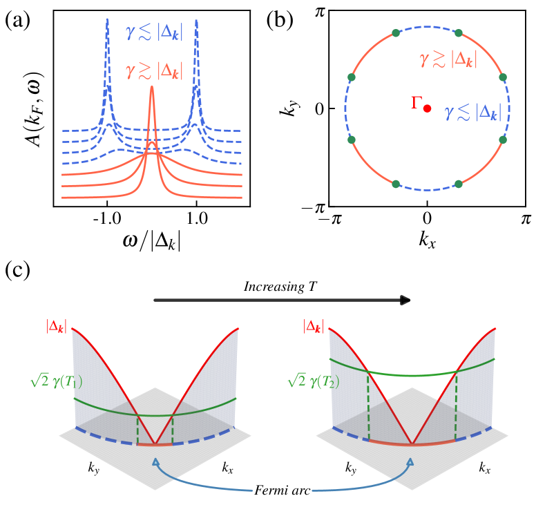
Figure 1:
(a) Spectral weights for varying values of ,
after setting .
(b) Schematic plot of the formation of Fermi arcs (for simplicity we adopt a circular Fermi surface).
(c) Evolution of Fermi arcs with increasing temperatures.
The theoretical analysis on the phase fluctuations starts from a phenomenological Hamiltonian with a generic superconducting pairing
.
The superconducting order parameter has an intrinsic momentum dependence
,
where denotes the form factor of pairing, e.g. for pairing.
We assume that:
(1) Due to the BKT nature of 2D superconducting transition, the phase fluctuations of dominate in the low-energy theory, and its amplitude maintains the mean-field value .
This is partially supported by the anomalously small superfluid density in 2D superconductors [27, 28, 29], e.g. cuprates.
The small value of results in the temperature associated with phase fluctuations being of the same order as the superconducting temperature ,
which suggests that the phase fluctuations play a crucial role in the thermodynamics near .
(2) The superconducting fluctuation in the temporal direction is neglectable compared with the spatial one.
Namely, we consider here only the static fluctuations of superconductivity.
This can be argued from the fact that the spatial correlation length diverges in the vicinity of BKT transition,
while the correlation in the imaginary-time direction is bounded by a finite inverse temperature .
Hence for the low-energy theory with a cutoff length scale satisfying , all the temporal fluctuations of are effectively integrated out.
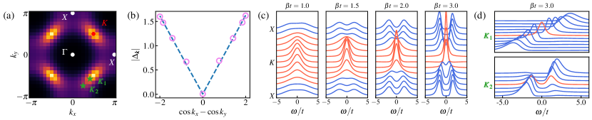
Figure 2:
Observations of Fermi arcs in DQMC.
(a) Green’s function as an estimation of the single-particle spectral function with lattice size and temperature ,
which is well below the superconducting transition. The nodal point is labeled as , and the anti-nodal point as .
(b) -wave gap function extracted from the low-temperature BCS gap in the single-particle spectrum.
(c) Single-particle spectral function along the node-antinode line -- for varying temperatures.
The red curves outline the shape of Fermi arcs, and the length of Fermi arcs grows with increasing temperature.
(d) Single-particle spectral function along the path perpendicular to the Fermi surface with temperature .
The momentum paths intersect with the Fermi surface at and respectively, marked out as the green stars in Fig. 2(a).
At this temperature, belongs to the Fermi arc while the spectrum at is gapped.
Under these assumptions, we can regard the fluctuating superconducting order parameters as a disordered background.
With certain fixed configurations of , one unambiguously solves the bilinear Hamiltonian by perturbative expansion over (assume ).
The effect of phase fluctuations is taken into account after averaging over the fluctuating configurations of
using the conditions of disorder averaging,
and ,
where is a function that exponentially decays from to 0 when .
For generic 2D superconductors, the superconducting transition falls into the BKT universality class,
and as a consequence, follows the BKT scaling of [30, 31],
where is a non-universal constant and represents the reduced temperature.
Following the scheme outlined above, we can evaluate any single-particle quantity using the perturbation theory.
For details of the theoretical analysis, readers may refer to Refs. [16, 32].
We firstly consider the electronic self-energy, which turns out to possess an intuitive form in the vicinity of superconducting where ,
(1)
For the -wave case, we define the superconducting gap and .
Eq. (1) describes a standard BCS-like self-energy corrected by a finite lifetime of Cooper pairs, denoted as a finite imaginary part of self-energy.
We will see that this scattering process of Cooper pairs naturally provides a unified description of the crossover from the BCS theory to the high-temperature Fermi liquid.
Consider the electrons carrying Fermi momenta and satisfying , the retarded Green’s function has complex poles at
[32],
with .
The real component of the pole denotes the frequency of quasiparticles,
and the imaginary one represents the inverse lifetime.
For temperatures close to the superconducting transition where ,
the phase fluctuations are too frail to smear the BCS picture, hence the Cooper pairs still survive up to an inverse lifetime ,
with two Green’s function poles at opposite frequencies.
At high temperatures with severe phase fluctuations and ,
the quasiparticle gets settled at the Fermi energy , which corresponds to a Fermi liquid.
Tuning up the strength of fluctuations , i.e. increasing temperature from , the system undergoes a smooth crossover from the BCS physics to a Fermi liquid state, see Fig. 1(a).
We further find that in the intermediate regime of the crossover,
the pair-scattering causes the broadening of single-particle spectrum, accounting for the evolution of pseudogap and Fermi arcs.
A straightforward calculation [32] reveals that for the pseudogap emerges in the single-particle spectrum,
and completely closes when ,
which is slightly smaller than because of the finite broadening of BCS peaks.
This analysis intuitively leads to the Fermi arcs as shown in Fig. 1(b)-(c).
Considering electrons labeled by the Fermi momentum, the pair-scattering rate varies only gently via the Fermi velocity , given the correlation length .
For those momenta near anti-nodes which experience large and , the spectrum is pseudogapped.
Otherwise, for those momenta near the nodes, the spectrum becomes gapless and metallic.
As temperature increases, the strong phase fluctuations lead to a decrease in and a significant increase in , causing the arcs to grow, see Fig. 1(c), until the large Fermi surface is recovered eventually.
The discussion above establishes a universal connection between phase fluctuations, pseudogap, and Fermi arcs for 2D nodal superconductors.
Numerical studies.—
To support the theoretical arguments above, here we numerically verify our predictions in a concrete lattice model.
The model we borrow here is proposed by Xu and Grover in Ref. [33],
the ground state of which has been proved to exhibit a competition between nodal -wave superconductivity (dSC) and antiferromagnetism (AFM)
by applying determinant Quantum Monte Carlo (DQMC) simulations.
This model couples the electrons (), which live on the vertices of the square lattice,
to the fluctuating rotors which live on the nearest-neighbor bonds .
The Hamiltonian is given by ,
where
denotes the standard Hubbard model at half-filling with nearest-neighbor hoppings, and .
is the coupling between electrons and rotors in the -wave pairing channel,
where for bonds along the -axis and for bonds along the -axis.
rules the dynamics of rotors
and a self-interaction term is included resembling that in the quantum rotor model [34],
where is the canonical momentum.
It is shown in Ref. [33] that this model is free of the infamous sign problem due to the presence of an anti-unitary symmetry [35],
and a complete phase diagram of the ground state is established which supports competing dSC and AFM.
To search for the Fermi arcs and evaluate the role of phase fluctuations, we simulate the model at finite temperatures using DQMC.
Details about the DQMC algorithm and its implementation to this model can be found in [36, 32].
Unless otherwise specified, we set the imaginary-time spacing equal to for maintaining a controllable systematic error and work with lattice sizes ranging from 8 to 24.
For all our presented results, we set , , and .
According to [33], this set of parameters realizes a nodal -wave superconductor, and importantly, there is no presence of long-range magnetic order in the ground state.
In Fig. 2 we show the formation of Fermi arcs in the electronic single-particle spectrum at finite temperature.
The single-particle spectra are extracted from the imaginary-time Green’s functions, which are computed using the stochastic analytic continuation (SAC) method [37, 38].
As shown in Fig. 2(c), the well-defined nodal gap manifests itself in the single-particle spectrum at low temperature ,
and the extraction of the gap function in Fig. 2(b) confirms that the superconducting gap indeed possesses a symmetry.
For increasing temperatures, the Fermi arcs spread out to the antinodes, illustrated as red curves in Fig. 2(c),
and this can be explained by the proliferation of phase fluctuations following our analysis in the previous section.
To quantify the superconducting fluctuations, we first identify the -wave superconductivity and locate the superconducting transition
through measuring the -wave pairing order parameter ,
and the static -wave pairing correlation function .
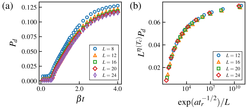
By applying data collapse (Fig. 3), we determine the superconducting BKT transition at and the correlation function with .
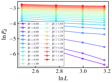
Figure 3:
Data collapse to determine the BKT transition temperature and superconducting correlation length .
(a) -wave pairing correlation function versus varying inverse temperature .
(b) Data collapse of -wave pairing correlation .
We have fixed the critical exponent for the BKT transition [30, 31],
and obtained and .
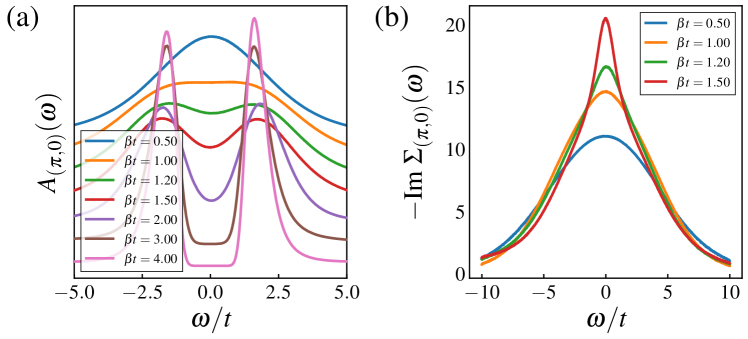
Figure 4:
(a) Antinode pseudogap extracted using SAC. The inverse temperature ranges from 0.5 to 4, with .
(b) Electronic self-energy computed from the single-particle spectrum in Fig. 4(a).
In order to benchmark with the theoretical self-energy in Eq. (1) directly, we calculate the electronic self-energy
from the single-particle spectrum obtained by SAC.
By noting that , we first compute based on the Kramers-Kronig relation,
and relate the self-energy to the complex Green’s function via .
Fig. 4 shows the recovered single-particle spectrum at the antinode, and the corresponding self-energy evaluated.
It is inspiring that the imaginary part of the self-energy indeed behaves as what we expected theoretically in Eq. (1).
For antinodal fermions, peaks significantly at the Fermi energy with a finite broadening
growing up with increasing temperatures, due to the scattering of Cooper pairs.
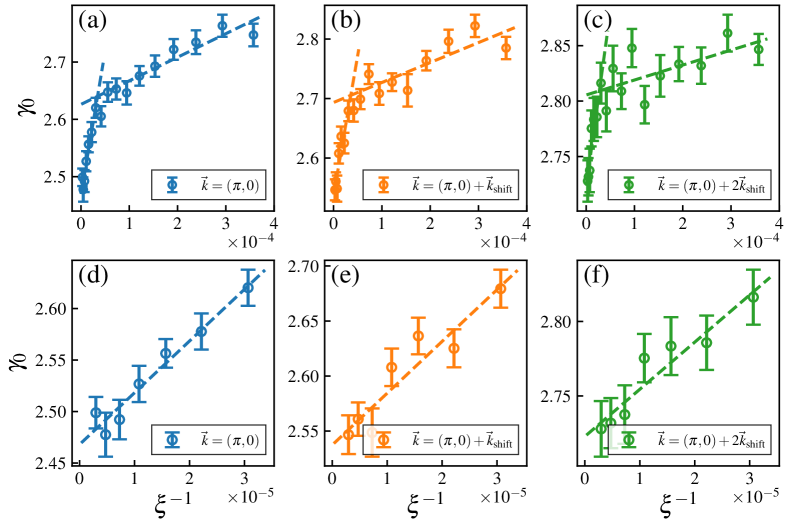
Figure 5:
Cooper pair scattering rate extracted by fitting the electronic self-energy.
The DQMC data contributing to the evaluation of self-energy are obtained on an lattice with and ranging from 0.7 to 0.9.
We focus on the momenta in the neighborhood of antinodes, e.g. ,
and the shift of moment reads .
Figs. 5(d)-(f) is the zoom-in to the small region of the same data shown in Figs. 5(a)-(c).
For all the fittings, remains small with a weak temperature dependence, which we do not present here.
We fit the self-energy according to the fitting formula ,
which quite resembles that in Eq. (1) with for the antinode.
is interpreted as the pair-scattering in our theory
while can be regarded as a Fermi-liquid-like renormalization,
and denotes the renormalized superconducting gap.
It turns out that this form of self-energy is also widely accepted as a working-assumption in dealing with angle-resolved photoemission data of realistic high- materials [39, 40].
In Fig. 5 we plot the fittings of versus the inverse correlation length for momenta near the antinodes.
Overall speaking, has a positive relation to the inverse correlation length over a large temperature range.
A linear relationship between and is found in Figs. 5(d)-(f) for temperatures close to ,
as we expected for the scattering induced by phase fluctuations where .
On the other hand, the slope of versus gradually decreases as the temperature grows, as shown in Fig. 5(a)-(c).
In this regime, our theory may cease to be effective if decays too fast to several lattice constants, which contradicts our theoretical assumption .
(Although the presented in Fig. 5 remains large numerically, note that we can only determine up to a non-universal factor.)
Besides, we can not exclude the effect of short-ranged spin-density-wave (SDW), which is possibly presented at finite temperatures although the ground state exhibits no long-range magnetic order.
Since the Fermi surface of our model has perfect nesting,
the scattering of short-ranged SDW makes identical and inseparable contributions to the self-energy compared with the scattering of fluctuating superconductivity.
This may account for the additional broadening in and above the superconducting phase,
causing gradual deviations from a linear relation as in Fig. 5.
In conclusion, the broadening of self-energy in Fig. 4(b) and its dependence on the superconducting correlation length in Fig.5 together validate our theory qualitatively, at least in the vicinity of .
Conclusion and Discussions.—
In summary, we propose that quite generally for 2D superconductors,
the strong phase fluctuations above mediate a well-defined scattering process for the Cooper pairs,
leading to ubiquitous pseudogap in the electronic single-particle spectrum.
Further for nodal -wave superconductors, the interplay of phase fluctuations and nodal quasiparticles leads to the Fermi arcs in a quite general manner.
We also confirm our theoretical predictions by performing an unbiased DQMC study on a lattice model
hosting a nodal -wave superconducting ground state and observing Fermi arcs at finite temperatures.
The research methodology we followed here implies a reliable approach to analyzing phase fluctuations with generic superconducting pairing,
and can get readily extended to problems concerning static disorders or other fluctuating orders at finite temperatures, e.g. the short-ranged SDW.
It is also surprising that one can understand the formation of Fermi arcs and superconducting fluctuations in such a unified and concise picture.
To fully figure out the evolution of Fermi arcs, it is of great interest to study the coexisting superconducting and SDW fluctuations from both theoretical and computational perspectives,
which will guide our future work.
Acknowledgements.
Acknowledgements.—
Y.Q. is supported by National Natural Science Foundation of China (NSFC) through Grant Nos. 11874115 and 12174068.
X.Y.X. acknowledges the support of National Key R&D Program of China (Grant No. 2022YFA1402702, No. 2021YFA1401400), the National Natural Science Foundation of China (Grants No. 12274289), Shanghai Pujiang Program under Grant No. 21PJ1407200, the Innovation Program for Quantum Science and Technology (under Grant no. 2021ZD0301900), Yangyang Development Fund, and startup funds from SJTU.
The authors also appreciate Beijing PARATERA Tech Co., Ltd. for providing the HPC resources which have contributed to the computational results presented in this work.
Marshall et al. [1996]D. S. Marshall, D. S. Dessau, A. G. Loeser, C.-H. Park, A. Y. Matsuura, J. N. Eckstein, I. Bozovic, P. Fournier, A. Kapitulnik, W. E. Spicer, and Z.-X. Shen, Phys. Rev. Lett. 76, 4841 (1996).
Kang et al. [2020]B. L. Kang, M. Z. Shi, S. J. Li, H. H. Wang, Q. Zhang, D. Zhao, J. Li, D. W. Song, L. X. Zheng, L. P. Nie, T. Wu, and X. H. Chen, Phys. Rev. Lett. 125, 097003 (2020).
Faeth et al. [2021]B. D. Faeth, S.-L. Yang, J. K. Kawasaki, J. N. Nelson, P. Mishra, C. T. Parzyck, C. Li, D. G. Schlom, and K. M. Shen, Phys. Rev. X 11, 021054 (2021).
Zhou et al. [2013]B. B. Zhou, S. Misra, E. H. Da Silva Neto, P. Aynajian, R. E. Baumbach, J. D. Thompson, E. D. Bauer, and A. Yazdani, Nature Physics 9, 474 (2013).
Gyenis et al. [2018]A. Gyenis, B. E. Feldman, M. T. Randeria, G. A. Peterson, E. D. Bauer, P. Aynajian, and A. Yazdani, Nat. Commun. 9, 549 (2018).
Oh et al. [2021]M. Oh, K. P. Nuckolls, D. Wong, R. L. Lee, X. Liu, K. Watanabe, T. Taniguchi, and A. Yazdani, Nature 600, 240 (2021).
Yoshida et al. [2003]T. Yoshida, X. J. Zhou, T. Sasagawa, W. L. Yang, P. V. Bogdanov, A. Lanzara, Z. Hussain, T. Mizokawa, A. Fujimori, H. Eisaki, Z.-X. Shen, T. Kakeshita, and S. Uchida, Phys. Rev. Lett. 91, 027001 (2003).
Kanigel et al. [2006]A. Kanigel, M. R. Norman, M. Randeria, U. Chatterjee, S. Souma, A. Kaminski, H. M. Fretwell, S. Rosenkranz, M. Shi, T. Sato, T. Takahashi, Z. Z. Li, H. Raffy, K. Kadowaki, D. Hinks, L. Ozyuzer, and J. C. Campuzano, Nat. Phys. 2, 447 (2006).
Kanigel et al. [2007]A. Kanigel, U. Chatterjee, M. Randeria, M. R. Norman, S. Souma, M. Shi, Z. Z. Li, H. Raffy, and J. C. Campuzano, Phys. Rev. Lett. 99, 157001 (2007).
Kondo et al. [2015]T. Kondo, W. Malaeb, Y. Ishida, T. Sasagawa, H. Sakamoto, T. Takeuchi, T. Tohyama, and S. Shin, Nat. Commun. 6, 7699 (2015).
Keimer et al. [2015]B. Keimer, S. A. Kivelson, M. R. Norman, S. Uchida, and J. Zaanen, Nature 518, 179 (2015).
Uemura et al. [1989]Y. J. Uemura, G. M. Luke, B. J. Sternlieb, J. H. Brewer, J. F. Carolan, W. N. Hardy, R. Kadono, J. R. Kempton, R. F. Kiefl, S. R. Kreitzman, P. Mulhern, T. M. Riseman, D. L. Williams, B. X. Yang, S. Uchida, H. Takagi, J. Gopalakrishnan, A. W. Sleight, M. A. Subramanian, C. L. Chien, M. Z. Cieplak, G. Xiao, V. Y. Lee, B. W. Statt, C. E. Stronach, W. J. Kossler, and X. H. Yu, Phys. Rev. Lett. 62, 2317 (1989).
[32]See Supplemental Material at URL for technical details about the self-energy evaluation, pseudogap in the single-particle spectrum, the determinant Quantum Monte Carlo implementation, determination of BKT transition point, and the stochastic analytic continuation calculation .
Assaad and Evertz [2008]F. Assaad and H. Evertz, Computational Many-Particle Physics, edited by H. Fehske, R. Schneider, and A. Weiße, Lecture Notes in Physics, Vol. 739 (Springer, Berlin, Heidelberg, 2008) pp. 277–356.
Shi et al. [2008]M. Shi, J. Chang, S. Pailhés, M. R. Norman, J. C. Campuzano, M. Månsson, T. Claesson, O. Tjernberg, A. Bendounan, L. Patthey, N. Momono, M. Oda, M. Ido, C. Mudry, and J. Mesot, Phys. Rev. Lett. 101, 047002 (2008).
Supplementary Material for “The interplay of phase fluctuations and nodal quasiparticles:
ubiquitous Fermi arcs in two-dimensional -wave superconductors”
I Perturbative Evaluation of the Electronic Self-energy
In this section, we deduce the electronic self-energy using disorder averaging and the perturbative theory.
Because the first order correction vanishes due to our disorder averaging condition ,
we focus on the second order self-energy correction, which can be read from the Feynman diagram in Fig. S1 as
(S1)
Figure S1:
Feynman diagram for the second-order self-energy correction.
The arrowed solid lines denote the fermionic propagators.
At the interaction vertex, marked by a cross, the particles flowing from the left and right carry opposite charges,
and a particle with momentum can get scattered into a hole with momentum .
This implies that the superconducting pairing in our phenomenological model conserves neither momentum nor charge.
The dashed lines and the crossed dot represent the disorder averaging over pairing correlation functions.
For a fixed configuration of superconducting order parameters , the translational invariance is broken,
and hence the self-energy Eq. (S1) depends on both incoming momentum and the outcoming one .
The Fourier-transformed superconducting order parameter is defined as
(S2)
where in the second step we have applied the relation .
Hereafter, we assume a -wave pairing ,
but note that a similar analysis can be applied to deal with generic forms of pairing.
For the convenience of analytic calculations and without losing of generality,
we adopt a Gaussian decay function for the disorder-averaged pairing correlation,
and express it in the momentum representation as
(S3)
Substituting this result into Eq. (S1), we obtain with
(S4)
From Eq. (S4) one can already realize that the self-energy acquires a finite imaginary component caused by the phase fluctuations,
which exactly corresponds to the inverse lifetime of Cooper pairs.
This can be brought out explicitly by further diving into the limit of large correlation length , i.e. near the superconducting transition ,
and examining the imaginary part of self-energy,
(S5)
In the first step, we use the identity ,
and then substitute with before we further absorb it into
by noting that the integrand takes a significant value only near the small region around cut off by .
In the second step, one can exactly solve the integral over by assuming a free dispersion and is the zero-order modified Bessel function of the first kind.
The asymptotic form of in the limit of is adopted in the last step,
and we finally find that the imaginary part of self-energy obeys a Gaussian distribution with a peak positioned at and a standard deviation .
This observation on motivates us to rewrite the self-energy into
(S6)
which is exactly what we have announced in the main text.
The imaginary part of Eq. (S6) turns out to obey a Lorentz distribution compared with the Gaussian one in Eq. (S5).
It is very hopeful that Eq. (S4) and Eq. (S6) will produce similar low-energy properties in the neighborhood of superconducting transition .
To see this, both the real and imaginary parts of Eq. (S4) and Eq. (S6) are benchmarked numerically in Fig. S2,
where good agreements are achieved for .
We argue that for any specific form of two-point correlation, imposed by the disorder averaging condition with a well-defined correlation length ,
the detailed high-energy information of the correlation decay is irrelevant to the system’s thermodynamics in the vicinity of and can hardly be probed.
Under this assumption, a similar analysis as we outline above applies to generic correlations,
and it is generally expected that the low-energy physics is well described by the self-energy in Eq. (S6).
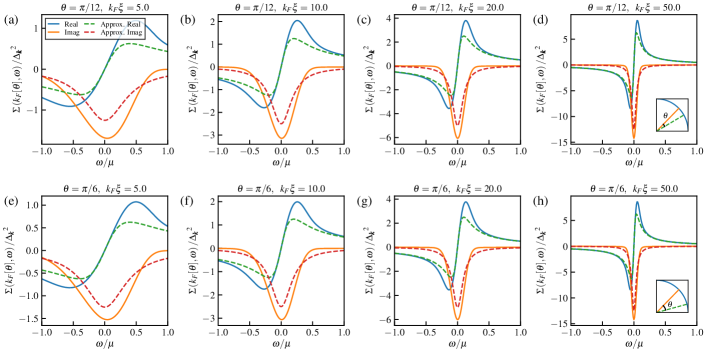
Figure S2:
Benchmarks of self-energy in Eq. (S4) and Eq. (S6)
by varying both the correlation length and the angle between the node and momentum , which is illustrated in the mini chart of the rightmost figure.
The exact self-energy Eq. (S4) is plotted in the solid line and the approximated one Eq. (S6) in the dashed line.
It is found that Eq. (S6) produces similar real and imaginary components as Eq. (S4) especially when blows up.
We also test the results for momenta away from the Fermi surface, which are generally a translation of the results above, and hence we do not show them separately.
II Evolution of the Electronic Single-particle Spectrum and Pseudogap
The retarded Green’s function follows straightforwardly from the self-energy in Eq. (S6) as
(S7)
where we define as the nodal BCS dispersion.
The pole of Green’s function reflects the dispersion of emergent quasiparticles,
which can be readily read from Eq. (S7).
The single-particle spectral function can be evaluated from as
(S8)
and for the Fermi momentum where ,
(S9)
By examining the denominator of Eq. (S9), it is easy to find that approaches its maximum value when
(S10a)
(S10b)
According to this, we define the energy scale of pseudogap .
It is realized that the spectral gap remains open above superconducting unless .
The smooth crossover from the BCS quasiparticle picture to the Fermi liquid at high temperature, i.e. the pseudogap, is shown in Fig. S3.
Close to the superconducting temperature, i.e. ,
we infer from Eq. (S9) that
with the broadening of BCS peaks characterized by .
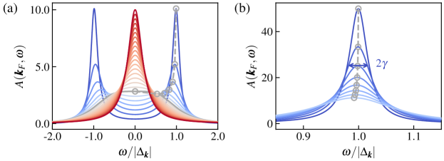
Figure S3:
Single-particle spectral function at the Fermi momentum for varying .
We outline the spectral peaks at using the dashed line with circles.
(a) The crossover from the BCS physics to the Fermi liquid
with ranging from 0.1 to 2.5.
The intermediate region corresponds to the onset of pseudogap, which gets completely closed when , i.e., the gray solid curve.
(b) Broadening of the BCS quasiparticle peak, e.g., the one near , for ranging from 0.02 to 0.1.
The two-sided arrow implies that the spectrum acquires a half-width proportional to .
III Determinant Quantum Monte Carlo Implementation
III.1 Basic Formalism of Determinant Quantum Monte Carlo
We here transcribe our lattice model as follows
(S11a)
(S11b)
(S11c)
(S11d)
To investigate the thermodynamic properties of this model, we apply determinant Quantum Monte Carlo (DQMC) simulation at finite temperatures.
It is insightful to first switch to the particle-hole channel, and reformulate the model Hamiltonian on the square lattice
with a basis transformation , which leads to
(S12a)
(S12b)
(S12c)
(S12d)
where denotes the density operator.
In the framework of DQMC and given the partition function ,
one divides the imaginary-time evolution into slices with imaginary-time spacing .
We further decompose the exponent of at time slice into more sectors, where different sectors basically do not commute.
This can be accomplished by using Trotter decomposition at the cost of an accompanying systematic error of order , as in Eq. (S13),
(S13)
To analytically integrate out the fermionic degrees of freedom, one needs to transform the two-body interaction term into fermion bilinears under the Hubbard-Stratonovich (HS) transformation.
The resulting fermion bilinears are coupled to certain auxiliary bosonic fields , which take values in . [41]
(S14)
where enumerates the lattice sites, , , , , and .
This particular scheme of HS transformation preserves the spin symmetry and introduces a systematic error of order when measuring physical observables, which is, however, neglectable compared with the Trotter error.
To deal with the bosonic rotor fields in the path integral formalism,
it is convenient to adopt the bosonic coherent state representation satisfying for all bonds .
Under this representation, we need to estimate the matrix element .
This can be achieved by inserting completeness relations of the angular momentum eigenstates and applying the Poisson summation formula [42].
As a result, under the Villain approximation, we finally get
(S15)
After these preparations, we are ready to evaluate the partition function in Eq. (S13).
First of all, we trace out the bosonic fields using Eq. (S15) and the definition of coherent states,
(S16)
where we have mapped the quantum rotor term into a 3D anisotropic XY model in the path integral level.
Furthermore, we trace out the fermion bilinears using Eq. (S14),
(S17)
with the constant prefactor omitted.
In Eq. (S17), denotes our fermionic basis,
and the three matrices , , satisfy that , , and .
matrix is defined as .
For fermion bilinears, the identity holds.
To conclude, by identifying the configurations as , the partition function reads with
(S18a)
(S18b)
One can verify that , , stay invariant under the anti-unitary transformation : , , as mentioned in the main text.
This guarantees that the determinant in Eq. (S18b) is positive for any and the sign problem does not appear [35].
III.2 Monte Carlo Updating Schemes
We adopt the local updating scheme to update the auxiliary field configuration .
Both and fields are picked up and changed randomly in a trail local update.
The accepting ratio of the new configuration is given by
(S19)
where the ratio can be calculated trivially.
To evaluate , a nice result holds
(S20)
where we define , and the equal-time Green’s function with .
We stress that the Green’s functions are crucial to both the Monte Carlo updates and the measurements of physical observables,
hence we shall carry them around throughout the entire simulation.
Once the new configuration is accepted, the Green’s function is updated accordingly as
(S21)
For local updates, possesses a quite sparse structure: e.g. for local update , it has only two non-zero diagonal elements;
and for the update of rotor , also involves a limited number of elements, which does not scale with the system size ,
after we apply the checkerboard breakups when multiplying .
Due to the sparseness of , the locally updated Green’s function can be evaluated efficiently using
Eq. (S21) and the Sherman-Morrison-Woodbury formula [36].
Apart from the local updates, we also develop a global updating scheme to update the rotors by cluster.
Because the rotor fields serve as the order parameter describing the symmetry breaking of superconductivity,
the simulation under the local updating scheme suffers from the critical slowing down, especially in the superconducting phase at low temperatures.
To address this problem, we embed the Wolff algorithm [43, 44] into the general framework of DQMC.
The steps for the global updating scheme are as follows:
•
Randomly select certain rotor field as the starting point for growing the cluster.
•
Grow the rotor cluster in both the spatial and temporal direction according to the rotor-relevant weight in ,
using the standard Wolff algorithm [43].
•
To fulfill the detailed balance, the trial cluster update is accepted based on a probability given by
(S22)
where denotes the configuration after the cluster update.
Once the trial configuration is accepted, we update the cluster simultaneously.
This concludes a complete Wolff cluster update.
Note that after the global update, we need to compute the updated Green’s function from scratch, which is numerically expensive.
In practice, we always combine the global updating scheme with the local one, e.g. performing a batch of global updates after several local Monte Carlo sweeps over the complete space-time lattice.
In Fig. S4, we measure and benchmark the autocorrelation function for these two updating schemes.
It is found that, e.g. in the -wave superconducting (-SC) phase, the combined updating scheme with both local and Wolff cluster (WC) updates exhibits a much shorter autocorrelation time for rotor observables and a much shorter Markov time for the thermalization, compared with the pure local updating scheme.
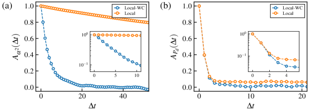
Figure S4:
Autocorrelation functions for the local updating scheme and the combined local-WC updating scheme.
The autocorrelation function for certain observable is defined as .
denotes the time difference in the Markov chain, and we measure the ‘time’ in the unit of a single Monte Carlo sweep,
where we scan over the complete space-time lattice for one time.
In the local-WC scheme, one Wolff cluster move is followed after one usual Monte Carlo sweep.
Measurements are performed in the -SC phase with parameters , , , , , and , where the local scheme typically suffers from the critical slowing down.
(a) Autocorrelation function for the static correlation function of rotors .
The insets show the semi-log plots of the same data, especially the exponentially decay part.
(b) Autocorrelation function for the static -wave pairing correlation function , which is defined in III.3.
We can see from Fig. 3(a) that by applying the local-WC scheme, the autocorrelation of , which explicitly depends on the rotors, is significantly suppressed.
However, it turns out that the fermionic observable, e.g. , is more sensitive to the discrete fields than the rotors,
hence applying cluster updates on rotors has a limited impact on the autocorrelation time of , as shown in Fig. S4(b).
III.3 Measurements
Both static and dynamic physical observables can be measured in DQMC by decomposing them into equal-time or time-displaced Green’s functions using Wick’s theorem.
A standard Monte Carlo sampling procedure then follows to estimate the expectation values of the observables.
In our context, in order to identify the -wave superconductivity, we define the -wave pairing order parameter ,
and measure the static -wave pairing correlation function ,
(S23)
where we have expressed the formula in the particle-hole channel, and identified the equal-time Green’s function as .
One then breaks up the quartic terms in Eq. (S23) into products of Green’s function using Wick’s theorem.
Another important observable we want to evaluate is the single-particle spectral function, through which we observe the formation of pseudogap and Fermi arcs directly.
Consider the time-displaced Green’s function in the momentum space,
(S24)
where
and .
The single-particle spectrum is related to the imaginary-time through an integral transform,
for obtaining which we perform the stochastic analytic continuation calculations, as we will introduce in Sec. V.
IV Determination of the BKT Transition Point
We perform finite-size scaling analysis to locate the BKT transition point.
The scaling of the -wave correlation function follows a BKT form [45]
(S25)
where denotes the reduced temperature, and is a universal scaling function.
For the BKT transition, the critical exponent .
At the transition point where diverges, we conclude from Eq. (S25) that .
In DQMC simulations, we measure the -wave correlation for varying temperatures and lattice sizes to obtain .
Fig. S5 shows the plot of versus for varying temperatures.
By requiring the slope of versus equals to , we locate the superconducting transition temperature as .
Fixing the value of and , one can then tune the non-universal factor to let the measured data collapse into a universal function,
and further obtain the correlation length , as we did in the main text.
Figure S5:
Double log plot of versus lattice size for varying temperatures.
V Stochastic Analytic Continuation Calculation
Technically, the evaluation of the single-particle spectrum from the imaginary-time Green’s function ,
defined on a discrete imaginary-time set , turns out to be a challenging task.
By definition, is related to through the following integral transform
(S26)
where denotes the integral kernel. For fermionic Green’s functions, .
It has long been realized that solving the inverse integral transform, i.e. obtaining from ,
appears to be an ill-posed problem, especially when ’s are estimated from the QMC simulations with statistical errors,
which makes the analytic continuation procedure numerically unstable.
To overcome this challenge, we apply the stochastic analytic continuation (SAC) [37] to obtain all the single-particle spectra presented in this work.
The combination of QMC and SAC has succeeded in producing reliable real-frequency spectral functions in many spin and fermionic models.
For interested readers, we refer to a recent review [38], which provides a comprehensive introduction to SAC.
The key spirit of SAC is to perform a Monte Carlo sampling procedure over the parametric space of .
The statistical weight of certain parametric configuration obeys a Boltzmann distribution as
(S27)
where quantifies the goodness of fitting between the QMC-measured Green’s functions and the ones fitted from the parameterized spectrum.
denotes the fictitious temperature to strike a balance between the minimization of and the thermal fluctuations which smoothen the spectrum.
In practice, one performs a simulated annealing procedure to lower adiabatically from a sufficiently high value.
Once the optimal is found, all statistically possible spectral configurations are sampled to produce the final results.