Quantum Bayesian Optimization

Zhongxiang Dai*1, Gregory Kang Ruey Lau*1,2, Arun Verma1, Yao Shu1,
Bryan Kian Hsiang Low1, Patrick Jaillet3
1
Department of Computer Science, National University of Singapore
2CNRS@CREATE, 1 Create Way, #08-01 Create Tower, Singapore 138602
3Department of Electrical Engineering and Computer Science, MIT
dzx@nus.edu.sg, greglau@comp.nus.edu.sg, arun@comp.nus.edu.sg,
shuyao95@u.nus.edu, lowkh@comp.nus.edu.sg, jaillet@mit.edu
Abstract

Kernelized bandits, also known as Bayesian optimization (BO), has been a prevalent method for optimizing complicated black-box reward functions. Various BO algorithms have been theoretically shown to enjoy upper bounds on their cumulative regret which are sub-linear in the number $T$ of iterations, and a regret lower bound of $\Omega(\sqrt{T})$ has been derived which represents the unavoidable regrets for any classical BO algorithm. Recent works on quantum bandits have shown that with the aid of quantum computing, it is possible to achieve tighter regret upper bounds better than their corresponding classical lower bounds. However, these works are restricted to either multi-armed or linear bandits, and are hence not able to solve sophisticated real-world problems with non-linear reward functions. To this end, we introduce the quantum-Gaussian process-upper confidence bound (Q-GP-UCB) algorithm. To the best of our knowledge, our Q-GP-UCB is the first BO algorithm able to achieve a regret upper bound of $\mathcal{O}(\text{poly}\log T)$, which is significantly smaller than its regret lower bound of $\Omega(\sqrt{T})$ in the classical setting. Moreover, thanks to our novel analysis of the confidence ellipsoid, our Q-GP-UCB with the linear kernel achieves a smaller regret than the quantum linear UCB algorithm from the previous work. We use simulations, as well as an experiment using a real quantum computer, to verify that the theoretical quantum speedup achieved by our Q-GP-UCB is also potentially relevant in practice.

1 Introduction

00footnotetext: * Equal contribution.

Kernelized bandits [9], also named Bayesian optimization (BO) [10, 11, 16, 19, 32], has been an immensely popular method for various applications involving the optimization of complicated black-box reward functions. For example, BO has been extensively used to optimize the hyperparameters of machine learning (ML) models [12, 14, 22], the parameters of computationally expensive simulators [5], etc. In every iteration $t=1,\ldots,T$, BO chooses an arm/input $x_{t}$ and then queries the reward function $f$ for a noisy observation $y_{t}=f(x_{t})+\zeta_{t}$ where $\zeta_{t}$ is a sub-Gaussian noise. In addition to its impressive practical performance, BO is also equipped with solid theoretical guarantees. A number of commonly adopted BO algorithms have been theoretically shown to enjoy sub-linear upper bounds on their cumulative regret [9, 33], which ensures that they are guaranteed to be able to find the global optimum of the reward function as $T$ (i.e., the total number of function queries) increases. On the other hand, a lower bound of $\Omega(\sqrt{T})$ (ignoring additional log factors) on the cumulative regret of BO has been shown [31], which represents the fundamental limit of any BO algorithm (in the classical setting). In other words, no classical BO algorithm can achieve a cumulative regret smaller than $\Omega(\sqrt{T})$. This naturally begs the question: can we leverage more advanced technology to go beyond the classical setting and hence break this fundamental limit of $\Omega(\sqrt{T})$? In this work, we give an affirmative answer by showing that this can be achieved with the aid of quantum computing [34].

Quantum bandits, which incorporates quantum computing into bandit algorithms, has been studied by a number of recent works [8, 38, 40, 41]. Notably, the recent work of [38] has introduced quantum variants of classical algorithms for multi-armed bandits (MAB) and stochastic linear bandits (SLB). In the setting of quantum bandits adopted by [38], every query to the reward function $f$ at the arm $x_{t}$ (in the classical setting) is replaced by a chance to access a quantum oracle, which encodes the reward distribution for the arm $x_{t}$. For every selected arm $x_{t}$, [38] has proposed to adopt the quantum Monte Carlo (QMC) algorithm [4, 28] as a subroutine to obtain an accurate estimation of $f(x_{t})$ in an efficient way, i.e., using a small number of queries to the quantum oracle (Lemma 1). As a result, [38] has shown that the regrets of the quantum algorithms for both MAB and SLB are significantly improved compared with their classical counterparts and are smaller than their classical lower bounds. However, both MAB and SLB fall short when optimizing complex real-world functions (e.g., optimizing the hyperparameters of ML models). This is because MAB is unable to exploit the correlations among the arms to model the reward function, and the assumption of a linear reward function adopted by SLB is usually too restrictive in practice. Therefore, designing a quantum bandit algorithm capable of optimizing sophisticated non-linear reward functions, which is a critical step towards practically useful quantum bandit algorithms, is still an open problem. In this work, we resolve this open problem by proposing the first algorithm for quantum BO.

Similar to [38], in our quantum BO problem setting, queries to the reward function in the classical setting are replaced by access to a quantum oracle encoding the reward distribution. As discussed in [38, 39], a quantum oracle is available when the learning environment is implemented by a quantum algorithm, which makes the setting of our quantum BO fairly general. For example, our quantum BO algorithm may be used to optimize the hyperparameters of quantum ML algorithms [3], such as quantum support vector machines (SVMs) [29], quantum neural networks (NNs) [1, 18], among others. It may also be used to optimize the parameters of simulators implemented on a quantum computer, or for applications involving quantum systems where the data produced is inherently quantum. Moreover, our quantum BO algorithm could also be applied to classical data and algorithms, because as discussed in [39], any classical computer program can be converted to a quantum circuit, allowing it to serve as a quantum oracle in our quantum BO algorithm.

In this work, we introduce the first quantum BO algorithm: quantum-Gaussian process-upper confidence bound (Q-GP-UCB). For every selected arm $x_{s}$, our Q-GP-UCB algorithm (Algo.Β 1) adopts the QMC subroutine (Lemma 1) to efficiently estimate the corresponding reward function value $f(x_{s})$ to satisfy a target estimation error $\epsilon_{s}$. Every arm $x_{s}$ is selected based on our weighted GP posterior distribution, in which every previously selected arm $x_{s}$ is given a weight of $1/\epsilon_{s}^{2}$ which is inversely related to its estimation error. The theoretical analysis of our Q-GP-UCB is faced with non-trivial technical challenges, and our contributions can be summarized as follows:

  • $\bullet$

    We analyze the growth rate of the weighted information gain (Sec.Β 5.1) which arises due to the use of our weighted GP regression (Sec.Β 4.1), and show its connection with the standard maximum information gain commonly used in the analysis of BO/kernelized bandits [9, 33]. Our analysis here may be of broader independent interest for future works adopting weighted GP regression.

  • $\bullet$

    We derive a tight confidence ellipsoid which gives a guarantee on the concentration of the reward function around the weighted GP posterior mean (Sec.Β 5.3), and discuss the intuition behind our proof which corresponds to an interesting interpretation about our Q-GP-UCB algorithm. A particularly crucial and novel step in our analysis relies on the recognition to apply the concentration inequality for 1-sub-Gaussian noise (Sec.Β 5.3).

  • $\bullet$

    We prove that our Q-GP-UCB achieves a regret upper bound of $\mathcal{O}(\text{poly}\log T)$ for the commonly used squared exponential (SE) kernel (Secs.Β 5.4 and 5.5), which is considerably smaller than the classical regret lower bound of $\Omega(\sqrt{T})$ [31] and hence represents a significant quantum speedup.

  • $\bullet$

    By using a similar proof technique to the one adopted for our tight confidence ellipsoid (Sec.Β 5.3), we improve the confidence ellipsoid for the quantum linear UCB (Q-LinUCB) algorithm [38]. This improved analysis leads to a tighter regret upper bound for Q-LinUCB, which matches the regret of our Q-GP-UCB with the linear kernel (Sec.Β 5.6).

  • $\bullet$

    We use simulations implemented based on the Qiskit package to verify the empirical improvement of our Q-GP-UCB over the classical GP-UCB and over Q-LinUCB, through a synthetic experiment and an experiment on automated machine learning (AutoML) (Sec.Β 6). Notably, we have also performed an experiment using a real quantum computer, in which our Q-GP-UCB still achieves a consistent performance advantage (Fig.Β 4, App.Β J)

2 Related Work

A number of recent works have studied bandit algorithms in the quantum setting. The works of [8] and [40] have focused on the problem of pure exploration in quantum bandits. [25] has studied a different problem setting where the learner aims to maximize some property of an unknown quantum state (i.e., the rewards) by sequentially selecting the observables (i.e., actions). The recent work of [38] has introduced algorithms for quantum multi-armed bandits (MAB) and stochastic linear bandits (SLB), and has shown that by incorporating the QMC subroutine into MAB and SLB, tight regret upper bounds can be achieved which are better than the classical lower bounds. More recently, the works of [23] and [41] have followed similar approaches to introduce quantum bandit algorithms for, respectively, stochastic convex bandits and bandits with heavy-tailed reward distributions. In addition to quantum bandits, some recent works have introduced quantum reinforcement learning (RL) algorithms. [39] has assumed access to a generative model of the environment and proved that their quantum RL algorithm achieves significantly better sample complexity over their classical counterparts. More recently, [17, 43] have removed the requirement for a generative model in quantum RL and achieved quantum speedup in terms of the regret. More comprehensive reviews of the related works on quantum RL can be found in recent surveys (e.g., [27]). The problem setting of our quantum BO (Sec.Β 3.2) is the same as many of these above-mentioned previous works on quantum bandits [38, 41] and quantum RL [17, 39, 43]. However, to the best of our knowledge, none of the existing works on quantum bandits (and quantum RL) is able to handle non-linear reward functions, which we resolve in this work. Over the years, extensive efforts [7, 24, 30, 36] have been made to design BO/kernelized bandit algorithms whose regret upper bounds are small enough to (nearly) match the classical regret lower bound of $\Omega(\sqrt{T})$ (ignoring additional log factors). Our work provides an alternative route by proving that with the aid of quantum computing, it is possible to achieve a tight regret upper bound which is significantly smaller than the classical regret lower bound.

3 Problem Setting and Background

3.1 Classical Kernelized Bandits

A BO/kernelized bandit algorithm aims to maximize a reward function $f\mathrel{\mathop{\mathchar 58\relax}}\mathcal{X}\rightarrow\mathbb{R}$ where $\mathcal{X}\subset\mathbb{R}^{d}$, i.e., it aims to find $x^{*}\in\arg\max_{x\in\mathcal{X}}f(x)$. Consistent with the previous works on BO/kernelized bandits [9, 37], we assume that $f$ lies in the reproducing kernel Hilbert space (RKHS) associated with a kernel $k$: $f\in H_{k}(\mathcal{X})$. That is, we assume that $\mathinner{\!\left\lVert f\right\rVert}_{H_{k}}\leq B$ for $B>0$, in which $\mathinner{\!\left\lVert\cdot\right\rVert}_{H_{k}}$ denotes the RKHS norm induced by the kernel $k$. Note that unlike previous works on linear bandits [2], our assumption here allows $f$ to be non-linear w.r.t.Β the input $x$. In this work, we mainly focus on the widely used squared exponential (SE) kernel: $k(x,x^{\prime})\triangleq\exp(-\mathinner{\!\left\lVert x-x^{\prime}\right\rVert}^{2}_{2}/(2l^{2}))$ in which $l$ is the length scale. We also extend our results to the MatΓ©rn kernel in Sec.Β 5.7. Without loss of generality, we assume that $k(\cdot,\cdot)\leq 1$. In the following, we use $[t]$ to denote $\{1,\ldots,t\}$ for simplicity.

In every iteration $t\in[T]$ of BO, an input $x_{t}$ is selected, after which a corresponding noisy observation $y_{t}=f(x_{t})+\zeta_{t}$ is collected where $\zeta_{t}$ is a sub-Gaussian noise (e.g., bounded noise or Gaussian noise). The inputs $x_{t}$’s are sequentially selected by maximizing an acquisition function, which is calculated based on the Gaussian process (GP) posterior distribution. Specifically, after $t$ iterations, we use the current history $\mathcal{D}_{t}\triangleq\{(x_{1},y_{1}),\ldots,(x_{t},y_{t})\}$ to calculate the GP posterior predictive distribution at $x\in\mathcal{X}$: $\mathcal{N}(\mu_{t}(x),\sigma^{2}_{t}(x))$ where

$$\begin{split}\mu_{t}(x)\triangleq k_{t}^{\top}(x)(K_{t}+\lambda I)^{-1}Y_{t},\quad\sigma^{2}_{t}(x)\triangleq k(x,x)-k_{t}^{\top}(x)(K_{t}+\lambda I)^{-1}k_{t}(x),\end{split}$$ (1)

in which $k_{t}(x)\triangleq[k(x_{\tau},x)]^{\top}_{\tau\in[t]}$ and $Y_{t}\triangleq[y_{x_{\tau}}]^{\top}_{\tau\in[t]}$ are column vectors, $K_{t}\triangleq[k(x_{\tau},x_{\tau^{\prime}})]_{\tau,\tau^{\prime}\in[t]}$ is the $t\times t$ covariance matrix, and $\lambda>1$ is a regularization parameter. Based on (1), a commonly used acquisition function is GP-UCB [33], which selects the next query by: $x_{t+1}=\arg\max_{x\in\mathcal{X}}\mu_{t}(x)+\xi_{t+1}\sigma_{t}(x)$ where $\xi_{t+1}$ is a parameter carefully chosen to balance exploration and exploitation. The performance of a BO/kernelized bandit algorithm is usually theoretically analyzed by deriving an upper bound on its cumulative regret: $R_{T}=\sum^{T}_{t=1}[f(x^{*})-f(x_{t})]$, and a tighter regret upper bound is an indicator of a better theoretical convergence.

3.2 Quantum Bandits/BO

A quantum state $|x\rangle$ in Hilbert space $\mathbb{C}^{n}$ can be expressed as a superposition of $n$ basis states (e.g. qubits) via a vector $\vec{x}=[x_{1},\ldots,x_{n}]^{\top}$, with $|x_{i}|^{2}$ representing the probability of being in the $i^{th}$ basis state. Given two quantum states $|x\rangle\in\mathbb{C}^{n}$ and $|y\rangle\in\mathbb{C}^{m}$, we use $|x\rangle|y\rangle=[x_{1}y_{1},\ldots,x_{n}y_{m}]^{\top}$ to denote their tensor product. A quantum algorithm typically works by applying unitary operators to quantum states, and may have access to input data encoded in unitary operators called quantum oracles (examples have been discussed in Sec.Β 1). We defer a more detailed introduction to quantum computing to related works dedicated to these topics (e.g., [26]).

Our quantum BO setting follows that of the quantum bandits works in [38, 41]. In every iteration of quantum BO, after an input $x$ is selected, instead of observing a noisy reward as in classical BO/bandits (Sec.Β 3.1), we get a chance to access a quantum unitary oracle $\mathcal{O}_{x}$ and its inverse that encode the noisy reward distribution. Specifically, let $P_{x}$ denote the reward distribution, $\Omega_{x}$ denote the finite sample space of $P_{x}$, and $y_{x}\mathrel{\mathop{\mathchar 58\relax}}\Omega_{x}\rightarrow\mathbb{R}$ denote the random reward associated with input $x$. Then, $\mathcal{O}_{x}$ is formally defined as:

$$\mathcal{O}_{x}\mathrel{\mathop{\mathchar 58\relax}}|0\rangle\rightarrow{\textstyle\sum}_{\omega\in\Omega_{x}}\sqrt{P_{x}(\omega)}|\omega\rangle|y_{x}(\omega)\rangle.$$ (2)

Quantum mean estimation, which aims to estimate the mean of an unknown distribution with better sample efficiency than classical algorithms, has been a widely studied problem [4, 21]. Consistent with the works of [38, 41], we will make use of the following quantum Monte Carlo (QMC) algorithm:

Lemma 1 (Quantum Monte Carlo (QMC) [28]).

Let $y_{x}\mathrel{\mathop{\mathchar 58\relax}}\Omega_{x}\rightarrow\mathbb{R}$ denote a random variable, $\Omega_{x}$ is equipped with probability measure $P_{x}$, and the quantum unitary oracle $\mathcal{O}_{x}$ encodes $P_{x}$ and $y_{x}$.

  • $\bullet$

    Bounded Noise: If the noisy output observation satisfies $y_{x}\in[0,1]$, then there exists a constant $C_{1}>1$ and a QMC algorithm $\text{QMC}(\mathcal{O}_{x},\epsilon,\delta)$ which returns an estimate $\hat{y}_{x}$ of $\mathbb{E}[y_{x}]$ such that $\mathbb{P}(|\hat{y}_{x}-\mathbb{E}[y_{x}]|>\epsilon)\leq\delta$, using at most $\frac{C_{1}}{\epsilon}\log(1/\delta)$ queries to $\mathcal{O}_{x}$ and its inverse.

  • $\bullet$

    Noise with Bounded Variance: If the variance of $y_{x}$ is $\leq\sigma^{2}$, then for $\epsilon<4\sigma$, there exists a constant $C_{2}>1$ and a QMC algorithm $\text{QMC}(\mathcal{O}_{x},\epsilon,\delta)$ which returns an estimate $\hat{y}_{x}$ s.t. $\mathbb{P}(|\hat{y}_{x}-\mathbb{E}[y_{x}]|>\epsilon)\leq\delta$, using at most $\frac{C_{2}\sigma}{\epsilon}\log_{2}^{3/2}\left(\frac{8\sigma}{\epsilon}\right)\log_{2}(\log_{2}\frac{8\sigma}{\epsilon})\log\frac{1}{\delta}$ queries to $\mathcal{O}_{x}$ and its inverse.

The quantum query complexity of a quantum algorithm is usually measured by the number of queries to the quantum oracle [3, 38]. So, the sample complexities from Lemma 1 can be compared with that of classical Monte Carlo (MC) estimation. In the classical setting, it can be easily shown using concentration inequalities that MC estimation requires $\widetilde{\mathcal{O}}(1/\epsilon^{2})$ samples to reach a target mean estimation error of $\epsilon$. Therefore, the QMC algorithm (Lemma 1), which only needs $\widetilde{\mathcal{O}}(1/\epsilon)$ samples, achieves a quadratic reduction in the required number of samples. This dramatic improvement is crucial for the quantum speedup in terms of regrets achieved by our algorithm (Sec.Β 5.4).

During our Q-GP-UCB algorithm, after every input $x_{s}$ is selected, we will apply the QMC algorithm from Lemma 1 with the quantum oracle $\mathcal{O}_{x_{s}}$ to obtain an estimation $y_{s}$ of its reward $f(x_{s})$ (line 6 of Algo.Β 1). Of note, the above-mentioned equivalence between a query to the quantum oracle and a sample for classical MC mean estimation implies that a query to the quantum oracle $\mathcal{O}_{x}$ in quantum BO/bandits is equivalent to the pulling of an arm $x$ in classical BO/bandits. Therefore, the cumulative regret $R_{T}$ of our Q-GP-UCB algorithm is defined as the regret incurred after $T$ queries to the quantum oracle, which makes it amenable to comparisons with the regrets of classical algorithms.

4 Quantum Bayesian Optimization

In this section, we first introduce weighted GP regression (Sec.Β 4.1) which will be used by our Q-GP-UCB algorithm to calculate the acquisition function for input selection, and then describe our Q-GP-UCB algorithm (Sec.Β 4.2) in detail.

4.1 Weighted GP Posterior Distribution

In contrast to standard GP-UCB [33] which uses the standard GP posterior distribution (1) to calculate the acquisition function, our Q-GP-UCB makes use of a weighted GP posterior distribution. That is, we assign a weight to every previous observation. Specifically, after stage $s$ of our Q-GP-UCB (i.e., given π’Ÿsβ‰œ{(xΟ„,yΟ„)}Ο„βˆˆ[s]β‰œsubscriptπ’Ÿπ‘ subscriptsubscriptπ‘₯𝜏subscriptπ‘¦πœπœdelimited-[]𝑠\mathcal{D}_{s}\triangleq\{(x_{\tau},y_{\tau})\}_{{\tau}\in[s]}), we define the weight matrix Wsβ‰œdiag​(1/Ο΅12,…,1/Ο΅s2)β‰œsubscriptπ‘Šπ‘ diag1superscriptsubscriptitalic-Ο΅12…1superscriptsubscriptitalic-ϡ𝑠2W_{s}\triangleq\text{diag}(1/\epsilon_{1}^{2},\ldots,1/\epsilon_{s}^{2}). Wssubscriptπ‘Šπ‘ W_{s} is an $s\times s$ diagonal matrix, in which the $\tau^{\text{th}}$ diagonal element represents the weight $1/\epsilon_{\tau}^{2}$ given to the $\tau^{\text{th}}$ observation $(x_{\tau},y_{\tau})$. We will set $\epsilon_{\tau}=\widetilde{\sigma}_{\tau-1}(x_{\tau})/\sqrt{\lambda}$ (Sec.Β 4.2), i.e., $\epsilon_{\tau}$ is calculated using the weighted GP posterior standard deviation (3) (conditioned on the first ${\tau}-1$ observations) at $x_{\tau}$.

Define $K_{s}\triangleq[k(x_{\tau},x_{\tau^{\prime}})]_{\tau,\tau^{\prime}\in[s]}$ which is the $s\times s$-dimensional covariance matrix given the first $s$ observations, and define K~sβ‰œWs1/2​Ks​Ws1/2β‰œsubscript~𝐾𝑠superscriptsubscriptπ‘Šπ‘ 12subscript𝐾𝑠superscriptsubscriptπ‘Šπ‘ 12\widetilde{K}_{s}\triangleq W_{s}^{1/2}K_{s}W_{s}^{1/2} which is the weighted covariance matrix. Similarly, define ks​(x)β‰œ[k​(x,xΟ„)]Ο„βˆˆ[s]βŠ€β‰œsubscriptπ‘˜π‘ π‘₯subscriptsuperscriptdelimited-[]π‘˜π‘₯subscriptπ‘₯𝜏top𝜏delimited-[]𝑠k_{s}(x)\triangleq[k(x,x_{\tau})]^{\top}_{\tau\in[s]} and k~s​(x)β‰œWs1/2​ks​(x)β‰œsubscript~π‘˜π‘ π‘₯superscriptsubscriptπ‘Šπ‘ 12subscriptπ‘˜π‘ π‘₯\widetilde{k}_{s}(x)\triangleq W_{s}^{1/2}k_{s}(x). Denote the collection of output observations by Ysβ‰œ[yΟ„]Ο„βˆˆ[s]βŠ€β‰œsubscriptπ‘Œπ‘ subscriptsuperscriptdelimited-[]subscriptπ‘¦πœtop𝜏delimited-[]𝑠Y_{s}\triangleq[y_{\tau}]^{\top}_{\tau\in[s]}, and define Y~sβ‰œWs1/2​Ysβ‰œsubscript~π‘Œπ‘ superscriptsubscriptπ‘Šπ‘ 12subscriptπ‘Œπ‘ \widetilde{Y}_{s}\triangleq W_{s}^{1/2}Y_{s}. With these definitions, given π’Ÿssubscriptπ’Ÿπ‘ \mathcal{D}_{s}, our weighted GP posterior distribution at an input $x\in\mathcal{X}$ is a Gaussian distribution: 𝒩​(ΞΌ~s​(x),Οƒ~s2​(x))𝒩subscript~πœ‡π‘ π‘₯superscriptsubscript~πœŽπ‘ 2π‘₯\mathcal{N}(\widetilde{\mu}_{s}(x),\widetilde{\sigma}_{s}^{2}(x)), in which

$$\begin{split}\widetilde{\mu}_{s}(x)\triangleq\widetilde{k}_{s}^{\top}(x)(\widetilde{K}_{s}+\lambda I)^{-1}\widetilde{Y}_{s},\quad\widetilde{\sigma}^{2}_{s}(x)\triangleq k(x,x)-\widetilde{k}_{s}^{\top}(x)(\widetilde{K}_{s}+\lambda I)^{-1}\widetilde{k}_{s}(x).\end{split}$$ (3)

Note that the GP posterior mean ΞΌ~ssubscript~πœ‡π‘ \widetilde{\mu}_{s} above is equivalently the solution to the following weighted kernel ridge regression problem: ΞΌ~s=arg⁑minf∈Hk​(𝒳)β€‹βˆ‘Ο„=1s1ϡτ2​(yΟ„βˆ’f​(xΟ„))2+λ​βˆ₯fβˆ₯Hk2subscript~πœ‡π‘ subscript𝑓subscriptπ»π‘˜π’³subscriptsuperscriptπ‘ πœ11superscriptsubscriptitalic-ϡ𝜏2superscriptsubscriptπ‘¦πœπ‘“subscriptπ‘₯𝜏2πœ†superscriptsubscriptdelimited-βˆ₯βˆ₯𝑓subscriptπ»π‘˜2\widetilde{\mu}_{s}={\arg\min}_{f\in H_{k}(\mathcal{X})}\sum^{s}_{\tau=1}\frac{1}{\epsilon_{\tau}^{2}}(y_{\tau}-f(x_{\tau}))^{2}+\lambda\mathinner{\!\left\lVert f\right\rVert}_{H_{k}}^{2}. We give a more detailed analysis of the weighted GP posterior (3) in App.Β A. Weighted GP regression has also been adopted by previous works on BO such as [15]. However, our choice of the weights, algorithmic design and theoretical analyses all require significantly novel treatments.

4.2 Q-GP-UCB Algorithm

1:Β Β forΒ stage $s=1,2,\ldots$Β do
2:Β Β Β Β Β xs=arg⁑maxxβˆˆπ’³β‘ΞΌ~sβˆ’1​(x)+Ξ²s​σ~sβˆ’1​(x)subscriptπ‘₯𝑠subscriptπ‘₯𝒳subscript~πœ‡π‘ 1π‘₯subscript𝛽𝑠subscript~πœŽπ‘ 1π‘₯x_{s}={\arg\max}_{x\in\mathcal{X}}\widetilde{\mu}_{s-1}(x)+\beta_{s}\widetilde{\sigma}_{s-1}(x) (3).
3:Β Β Β Β Β Ο΅s=Οƒ~sβˆ’1​(xs)/Ξ»subscriptitalic-ϡ𝑠subscript~πœŽπ‘ 1subscriptπ‘₯π‘ πœ†\epsilon_{s}=\widetilde{\sigma}_{s-1}(x_{s})/\sqrt{\lambda}.
4:Β Β Β Β Β (a) $N_{\epsilon_{s}}=\frac{C_{1}}{\epsilon_{s}}\log(\frac{2\overline{m}}{\delta})$ (for bounded noise), or(b) $N_{\epsilon_{s}}=\frac{C_{2}\sigma}{\epsilon_{s}}\log_{2}^{3/2}\big{(}\frac{8\sigma}{\epsilon_{s}}\big{)}\log_{2}(\log_{2}\frac{8\sigma}{\epsilon_{s}})\log\frac{2\overline{m}}{\delta}$ (for noise with variance bounded by $\sigma^{2}$).
5:Β Β Β Β Β If βˆ‘k=1sNΟ΅k>Tsubscriptsuperscriptπ‘ π‘˜1subscript𝑁subscriptitalic-Ο΅π‘˜π‘‡\sum^{s}_{k=1}N_{\epsilon_{k}}>T, terminate the algorithm.
6:Β Β Β Β Β Run the $\text{QMC}(\mathcal{O}_{x_{s}},\epsilon_{s},\delta/(2\overline{m}))$ algorithm to query the quantum oracle of $x_{s}$ for the next $N_{\epsilon_{s}}$ rounds, and obtain $y_{s}$ as an estimate of $f(x_{s})$.
7:Β Β Β Β Β Update the weighted GP posterior (3) using $(x_{s},y_{s})$.
Algorithm 1 Q-GP-UCB

Our Q-GP-UCB algorithm is presented in Algo.Β 1.Β Q-GP-UCB proceeds in stages.Β In stage $s$, we first select the next input $x_{s}$ to query by maximizing the GP-UCB acquisition function calculated using the weighted GP posterior distribution (3) (line 2 of Algo.Β 1). Here $\beta_{s}\triangleq B+\sqrt{2(\widetilde{\gamma}_{s-1}+1+\log(2/\delta))}$ (more details in Sec.Β 5.3), in which $\delta\in(0,2/e]$ and $\widetilde{\gamma}_{s-1}\triangleq\frac{1}{2}\log(\text{det}(I+\frac{1}{\lambda}\widetilde{K}_{s-1}))$ is the weighted information gain (more details in Sec.Β 5.1). Next, we calculate Ο΅s=Οƒ~sβˆ’1​(xs)/Ξ»subscriptitalic-ϡ𝑠subscript~πœŽπ‘ 1subscriptπ‘₯π‘ πœ†\epsilon_{s}=\widetilde{\sigma}_{s-1}(x_{s})/\sqrt{\lambda} (line 3) and $N_{\epsilon_{s}}$ (line 4), in which $N_{\epsilon_{s}}$ depends on the type of noise and the value of $\epsilon_{s}$. Here $\overline{m}$ is an upper bound on the total number $m$ of stages which we will analyze in Sec.Β 5.2. Subsequently, unless the algorithm is terminated (line 5), we run the QMC algorithm (Lemma 1) to estimate $f(x_{s})$ by querying the quantum oracle of $x_{s}$ for $N_{\epsilon_{s}}$ rounds (line 6). The QMC procedure returns an estimate $y_{s}$ of the reward function value $f(x_{s})$, for which the estimation error is guaranteed to be bounded: $|y_{s}-f(x_{s})|\leq\epsilon_{s}$ with probability of at least $1-\delta/(2\overline{m})$. Lastly, we update the weighted GP posterior (3) using the newly collected input-output pair $(x_{s},y_{s})$, as well as its weight $1/\epsilon_{s}^{2}$ (line 7).

Of note, the value of $\epsilon_{s}$ is used for both (a) calculating the number $N_{\epsilon_{s}}$ of queries to the quantum oracle for $x_{s}$, and (b) computing the weight $1/\epsilon_{s}^{2}$ assigned to $(x_{s},y_{s})$ in the weighted GP regression (3) in the subsequent iterations. Regarding (a), our designs of $\epsilon_{s}$ and $N_{\epsilon_{s}}=\widetilde{\mathcal{O}}(1/\epsilon_{s})$ have an interesting interpretation in terms of the exploration-exploitation trade-off: In the initial stages, the weighted GP posterior standard deviation Οƒ~sβˆ’1​(xs)subscript~πœŽπ‘ 1subscriptπ‘₯𝑠\widetilde{\sigma}_{s-1}(x_{s}) and hence $\epsilon_{s}$ are usually large, which leads to a small number $N_{\epsilon_{s}}$ of queries for every $x_{s}$ and hence allows our Q-GP-UCB to favor the exploration of more unique inputs; in later stages, Οƒ~sβˆ’1​(xs)subscript~πœŽπ‘ 1subscriptπ‘₯𝑠\widetilde{\sigma}_{s-1}(x_{s}) and $\epsilon_{s}$ usually become smaller, which results in large $N_{\epsilon_{s}}$’s and hence causes our Q-GP-UCB to prefer the exploitation of a small number of unique inputs. Regarding (b), assigning a larger weight $1/\epsilon_{s}^{2}$ to an input $x_{s}$ with a smaller $\epsilon_{s}$ is reasonable, because a smaller $\epsilon_{s}$ indicates a smaller estimation error for $y_{s}$ as we explained above, which makes the observation $y_{s}$ more accurate and reliable for calculating the weighted GP regression (3).

Note that we have modified the original GP-UCB by querying every selected input $x_{s}$ multiple times, in order to make it amenable to the integration of the QMC subroutine. The recent work of [6] has also adapted BO to evaluate a small number of unique inputs while querying each of them multiple times. It has been shown [6] that the resulting BO algorithm preserves both the theoretical guarantee (i.e., the regret upper bound) and empirical performance of the original BO, while significantly reducing the computational cost. So, the findings from [6] can serve as justifications for our modification to GP-UCB. Also note that despite this similarity, [6] still focuses on the traditional setting (i.e., their regret upper bound is $R_{T}=\mathcal{O}(\gamma_{T}\sqrt{T})$) and their regret analyses are entirely different from ours.

5 Theoretical Analysis

Throughout our analysis, we condition on the event that $|f(x_{s})-y_{s}|\leq\epsilon_{s},\forall s=1,\ldots,m$. This event holds with probability of at least $1-\delta/2$, because we set the error probability in QMC (Lemma 1) to $\delta/(2\overline{m})$ in which $\overline{m}\geq m$ (see Theorem 2 for details). For simplicity, we mainly focus on the scenario of bounded noise (i.e., the observations are bounded within $[0,1]$, the first case of Lemma 1), because the theoretical analyses and insights about the other scenario of noise with bounded variance (i.e., the second case of Lemma 1) are almost identical (more details in Sec.Β 5.5).

5.1 Weighted Information Gain

To begin with, the following lemma (proof in App.Β B) gives an upper bound on the sum of the weights in all $m$ stages, which will be useful for upper-bounding the weighted information gain $\widetilde{\gamma}_{m}$.

Lemma 2.

Choose $\delta\in(0,2/e]$, then we have that βˆ‘s=1m1/Ο΅s2≀T2subscriptsuperscriptπ‘šπ‘ 11superscriptsubscriptitalic-ϡ𝑠2superscript𝑇2\sum^{m}_{s=1}1/\epsilon_{s}^{2}\leq T^{2}.

Denote by $\gamma_{T}$ the maximum information gain from any set of $T$ inputs: $\gamma_{T}\triangleq\max_{\{x_{1},\ldots,x_{T}\}\subset\mathcal{X}}\frac{1}{2}\log\det(I+\frac{1}{\lambda}K_{T})$, which is commonly used in the analysis of BO/kernelized bandit algorithms [9, 33]. Denote by $\widetilde{\gamma}_{m}$ the weighted information gain from all $m$ selected inputs in all stages: $\widetilde{\gamma}_{m}\triangleq\frac{1}{2}\log\det(I+\frac{1}{\lambda}\widetilde{K}_{m})$. Note that in the definition of $\widetilde{\gamma}_{m}$, we do not take the maximum over all sets of $m$ inputs, so $\widetilde{\gamma}_{m}$ still depends on the selected inputs $\mathcal{X}_{m}\triangleq\{x_{1},\ldots,x_{m}\}$. Also note that $\{\epsilon_{1},\ldots,\epsilon_{m}\}$ are known constants conditioned on $\mathcal{X}_{m}$. This is because the weighted GP posterior standard deviation Οƒ~sβˆ’1subscript~πœŽπ‘ 1\widetilde{\sigma}_{s-1} (3) does not depend on the output observations, so every Ο΅s=Οƒ~sβˆ’1​(xs)/Ξ»subscriptitalic-ϡ𝑠subscript~πœŽπ‘ 1subscriptπ‘₯π‘ πœ†\epsilon_{s}=\widetilde{\sigma}_{s-1}(x_{s})/\sqrt{\lambda} only depends on $\{x_{1},\ldots,x_{s}\}$. The next theorem gives an upper bound on $\widetilde{\gamma}_{m}$.

Theorem 1.

(a) Given $\mathcal{X}_{m}\triangleq\{x_{1},\ldots,x_{m}\}$, the growth rate of $\widetilde{\gamma}_{m}$ is the same as that of Ξ³βˆ‘s=1m1/Ο΅s2subscript𝛾subscriptsuperscriptπ‘šπ‘ 11superscriptsubscriptitalic-ϡ𝑠2\gamma_{\sum^{m}_{s=1}1/\epsilon_{s}^{2}}.
(b) $\widetilde{\gamma}_{m}\leq\gamma_{T^{2}}$.

We give the complete statement of result (a) in Theorem 8 (App.Β C), which presents the concrete growth rate. As stated by result (a), to obtain an upper bound on $\widetilde{\gamma}_{m}$, we simply need to firstly use the upper bound on $\gamma_{T}$ from previous works [35], and then replace the $T$ in this upper bound by βˆ‘s=1m1/Ο΅s2subscriptsuperscriptπ‘šπ‘ 11superscriptsubscriptitalic-ϡ𝑠2\sum^{m}_{s=1}1/\epsilon_{s}^{2}. Based on this, the result (b) has further upper-bounded βˆ‘s=1m1/Ο΅s2subscriptsuperscriptπ‘šπ‘ 11superscriptsubscriptitalic-ϡ𝑠2\sum^{m}_{s=1}1/\epsilon_{s}^{2} by $T^{2}$ through Lemma 2. Note that because Ο΅s=Οƒ~sβˆ’1​(xs)/λ≀1subscriptitalic-ϡ𝑠subscript~πœŽπ‘ 1subscriptπ‘₯π‘ πœ†1\epsilon_{s}=\widetilde{\sigma}_{s-1}(x_{s})/\sqrt{\lambda}\leq 1, we have that $1/\epsilon_{s}^{2}\geq 1$ and hence βˆ‘s=1m1/Ο΅s2β‰₯msubscriptsuperscriptπ‘šπ‘ 11superscriptsubscriptitalic-ϡ𝑠2π‘š\sum^{m}_{s=1}1/\epsilon_{s}^{2}\geq m. Therefore, our weighted information gain $\widetilde{\gamma}_{m}$ has a looser upper bound than $\gamma_{m}$. This intuitively implies that our weighted covariance matrix $\widetilde{K}_{m}$ is expected to contain more information than the original $K_{m}$, whose implication will be discussed again in Sec.Β 5.2. The proof of Theorem 1 (App.Β C) has followed the analysis of the information gain from [35]. Specifically, we have leveraged a finite-dimensional projection of the infinite-dimensional RKHS feature space, and hence upper-bounded the information gain in terms of the tail mass of the eigenvalues of the kernel $k$. The proof requires carefully tracking the impact of the weights $1/\epsilon_{s}^{2}$ throughout the analysis. Importantly, our Theorem 1 and its analysis may be of wider independent interest for future works which also adopt weighted GP regression (Sec.Β 4.1).

The growth rate of $\gamma_{T}$ has been characterized for commonly used kernels [35]. Based on these, the next corollary provides the growth rates of $\widetilde{\gamma}_{m}$ for the linear and squared exponential (SE) kernels.

Corollary 1.

For the linear and squared exponential (SE) kernels, we have that

Ξ³~m=π’ͺ​(d​logβ€‹βˆ‘s=1m1/Ο΅s2)=π’ͺ​(d​log⁑T)linear kernel,Ξ³~m=π’ͺ​(logd+1β€‹βˆ‘s=1m1/Ο΅s2)=π’ͺ​((log⁑T)d+1)SE kernel.formulae-sequencesubscript~π›Ύπ‘šπ’ͺ𝑑subscriptsuperscriptπ‘šπ‘ 11superscriptsubscriptitalic-ϡ𝑠2π’ͺ𝑑𝑇linear kernel,subscript~π›Ύπ‘šπ’ͺsuperscript𝑑1superscriptsubscript𝑠1π‘š1superscriptsubscriptitalic-ϡ𝑠2π’ͺsuperscript𝑇𝑑1SE kernel.\begin{split}\widetilde{\gamma}_{m}&=\mathcal{O}(d\log{\textstyle\sum}^{m}_{s=1}1/\epsilon_{s}^{2})=\mathcal{O}(d\log T)\qquad\text{linear kernel,}\\ \widetilde{\gamma}_{m}&=\mathcal{O}(\log^{d+1}{\textstyle\sum}_{s=1}^{m}1/\epsilon_{s}^{2})=\mathcal{O}((\log T)^{d+1})\qquad\text{SE kernel.}\end{split}

5.2 Upper Bound on The Total Number $m$ of Stages

The next theorem gives an upper bound on the total number of stages of our Q-GP-UCB algorithm.

Theorem 2.

For the linear kernel, our Q-GP-UCB algorithm has at most $m=\mathcal{O}(d\log T)$ stages. For the SE kernel, our Q-GP-UCB algorithm has at most $m=\mathcal{O}(\left(\log T\right)^{d+1})$ stages.

Note that for the linear kernel, our upper bound on $m$ matches that of the Q-LinUCB algorithm from [38] (see Lemma 2 from [38]). The proof of Theorem 2 is given in App.Β D, and here we give a brief sketch of the proof. For stage $s$, define Vsβ‰œΞ»β€‹I+βˆ‘Ο„=1s(1/ϡτ2)​ϕ​(xΟ„)​ϕ​(xΟ„)βŠ€β‰œsubscriptπ‘‰π‘ πœ†πΌsubscriptsuperscriptπ‘ πœ11superscriptsubscriptitalic-ϡ𝜏2italic-Ο•subscriptπ‘₯𝜏italic-Ο•superscriptsubscriptπ‘₯𝜏topV_{s}\triangleq\lambda I+\sum^{s}_{\tau=1}(1/\epsilon_{\tau}^{2})\phi(x_{\tau})\phi(x_{\tau})^{\top}, in which $\phi(\cdot)$ is the (potentially infinite-dimensional) RKHS feature mapping: $k(x,x^{\prime})=\phi(x)^{\top}\phi(x^{\prime})$. Intuitively, $\log\det V_{s}$ represents the amount of information contained in the first $s$ selected inputs $\{x_{1},\ldots,x_{s}\}$. As the first step in our proof, we prove that thanks to our choice of $\epsilon_{s}$ (line 3 of Algo.Β 1) and our design of the weights $1/\epsilon_{s}^{2}$, the amount of information $\log\det V_{s}$ is doubled after every stage: $\det V_{\tau+1}=2\det V_{\tau},\forall\tau=0,\ldots,m-1$. This allows us to show that $m\log 2=\log(\det(V_{m})/\det(V_{0}))$ where $V_{0}=\lambda I$. Next, we show that this term is also related to our weighted information gain: $\log(\det(V_{m})/\det(V_{0}))=2\widetilde{\gamma}_{m}$, which allows us to upper-bound $m$ in terms of $\widetilde{\gamma}_{m}$ and hence in terms of βˆ‘s=1m1/Ο΅s2subscriptsuperscriptπ‘šπ‘ 11superscriptsubscriptitalic-ϡ𝑠2\sum^{m}_{s=1}1/\epsilon_{s}^{2} (see Corollary 1). This eventually allows us to derive an upper bound on $m$ by using the fact that the total number of iterations (i.e., queries to the quantum oracles) is no larger than $T$. Therefore, the key intuition of the proof here is that as long as we gather a sufficient amount of information in every stage, we do not need a large total number of stages.

5.3 Confidence Ellipsoid

The next theorem proves the concentration of $f$ around the weighted GP posterior mean (3).

Theorem 3.

Let $\eta\triangleq 2/T$, $\lambda\triangleq 1+\eta$, and $\beta_{s}\triangleq B+\sqrt{2(\widetilde{\gamma}_{s-1}+1+\log(2/\delta))}$. We have with probability of at least $1-\delta/2$ that

|f​(x)βˆ’ΞΌ~sβˆ’1​(x)|≀βs​σ~sβˆ’1​(x),βˆ€s∈[m],xβˆˆπ’³.formulae-sequence𝑓π‘₯subscript~πœ‡π‘ 1π‘₯subscript𝛽𝑠subscript~πœŽπ‘ 1π‘₯formulae-sequencefor-all𝑠delimited-[]π‘šπ‘₯𝒳|f(x)-\widetilde{\mu}_{s-1}(x)|\leq\beta_{s}\widetilde{\sigma}_{s-1}(x),\qquad\forall s\in[m],x\in\mathcal{X}.

The proof of Theorem 3 is presented in App.Β E, and here we give a brief proof sketch. Denote by $\mathcal{F}_{s-1}$ the $\sigma$-algebra β„±sβˆ’1={x1,…,xs,ΞΆ1,…,ΞΆsβˆ’1}subscriptℱ𝑠1subscriptπ‘₯1…subscriptπ‘₯𝑠subscript𝜁1…subscriptπœπ‘ 1\mathcal{F}_{s-1}=\{x_{1},\ldots,x_{s},\zeta_{1},\ldots,\zeta_{s-1}\} where $\zeta_{k}=y_{k}-f(x_{k})$ is the noise. Recall that Ws1/2β‰œdiag​(1/Ο΅1,…,1/Ο΅s)β‰œsuperscriptsubscriptπ‘Šπ‘ 12diag1subscriptitalic-Ο΅1…1subscriptitalic-ϡ𝑠W_{s}^{1/2}\triangleq\text{diag}(1/\epsilon_{1},\ldots,1/\epsilon_{s}) (Sec.Β 4.1), and define $\zeta_{1\mathrel{\mathop{\mathchar 58\relax}}s}\triangleq[\zeta_{k}]_{k\in[s]}$. In the first part of the proof, we use the RKHS feature space view of the weighted GP posterior (3) (see App.Β A) to upper-bound |f​(x)βˆ’ΞΌ~sβˆ’1​(x)|𝑓π‘₯subscript~πœ‡π‘ 1π‘₯|f(x)-\widetilde{\mu}_{s-1}(x)| in terms of Οƒ~sβˆ’1​(x)subscript~πœŽπ‘ 1π‘₯\widetilde{\sigma}_{s-1}(x) and β€–Ws1/2​΢1:sβ€–((K~s+η​I)βˆ’1+I)βˆ’1subscriptnormsuperscriptsubscriptπ‘Šπ‘ 12subscript𝜁:1𝑠superscriptsuperscriptsubscript~πΎπ‘ πœ‚πΌ1𝐼1||W_{s}^{1/2}\zeta_{1\mathrel{\mathop{\mathchar 58\relax}}s}||_{((\widetilde{K}_{s}+\eta I)^{-1}+I)^{-1}}. Next, the most crucial step in the proof is to upper-bound β€–Ws1/2​΢1:sβ€–((K~s+η​I)βˆ’1+I)βˆ’1subscriptnormsuperscriptsubscriptπ‘Šπ‘ 12subscript𝜁:1𝑠superscriptsuperscriptsubscript~πΎπ‘ πœ‚πΌ1𝐼1||W_{s}^{1/2}\zeta_{1\mathrel{\mathop{\mathchar 58\relax}}s}||_{((\widetilde{K}_{s}+\eta I)^{-1}+I)^{-1}} in terms of $\widetilde{\gamma}_{s}$ by applying the self-normalized concentration inequality from Theorem 1 of [9] to 1-sub-Gaussian noise. This is feasible because (a) every Ο΅s=Οƒ~sβˆ’1​(xs)/Ξ»subscriptitalic-ϡ𝑠subscript~πœŽπ‘ 1subscriptπ‘₯π‘ πœ†\epsilon_{s}=\widetilde{\sigma}_{s-1}(x_{s})/\sqrt{\lambda} is $\mathcal{F}_{s-1}$-measurable, and (b) conditioned on $\mathcal{F}_{s-1}$, the scaled noise term ΞΆs/Ο΅ssubscriptπœπ‘ subscriptitalic-ϡ𝑠\zeta_{s}/\epsilon_{s} (in Ws1/2​΢1:ssuperscriptsubscriptπ‘Šπ‘ 12subscript𝜁:1𝑠W_{s}^{1/2}\zeta_{1\mathrel{\mathop{\mathchar 58\relax}}s}) is $1$-sub-Gaussian. The statement (a) follows because $\epsilon_{s}$ only depends on $\{x_{1},\ldots,x_{s}\}$ as we have discussed in Sec.Β 5.1. The statement (b) follows since our QMC subroutine ensures that every noise term $\zeta_{k}$ is bounded within $[-\epsilon_{k},\epsilon_{k}]$ (Sec.Β 4.2) because $|y_{k}-f(x_{k})|\leq\epsilon_{k}$ (with high probability). This suggests that conditioned on $\mathcal{F}_{s-1}$ (which makes $\epsilon_{s}$ a known constant as discussed above), ΞΆs/Ο΅ssubscriptπœπ‘ subscriptitalic-ϡ𝑠\zeta_{s}/\epsilon_{s} is bounded within $[-1,1]$ and is hence 1-sub-Gaussian.

This critical step in the proof is in fact also consistent with an interesting interpretation about our algorithm. That is, after $x_{s}$ is selected in stage $s$, we adaptively decide the number $N_{\epsilon_{s}}$ of queries to the quantum oracle in order to reach the target accuracy $\epsilon_{s}$ (line 4 of Algo.Β 1). This ensures that $|y_{s}-f(x_{s})|\leq\epsilon_{s}$ (with high probability), which guarantees that the noise ΞΆs=ysβˆ’f​(xs)subscriptπœπ‘ subscript𝑦𝑠𝑓subscriptπ‘₯𝑠\zeta_{s}=y_{s}-f(x_{s}) is (conditionally) $\epsilon_{s}$-sub-Gaussian. Moreover, note that the vector of observations Y~ssubscript~π‘Œπ‘ \widetilde{Y}_{s} used in the calculation of the weighted GP posterior mean (3) is Y~s=Ws1/2​Yssubscript~π‘Œπ‘ superscriptsubscriptπ‘Šπ‘ 12subscriptπ‘Œπ‘ \widetilde{Y}_{s}=W_{s}^{1/2}Y_{s}. So, from the perspective of the weighted GP posterior (3), every noisy observation $y_{s}$, and hence every noise ΞΆssubscriptπœπ‘ \zeta_{s}, is multiplied by $1/\epsilon_{s}$. So, the effective noise of the observations Y~ssubscript~π‘Œπ‘ \widetilde{Y}_{s} used in the weighted GP posterior (i.e., ΞΆs/Ο΅ssubscriptπœπ‘ subscriptitalic-ϡ𝑠\zeta_{s}/\epsilon_{s}) is $\epsilon_{s}/\epsilon_{s}=1$-sub-Gaussian. This shows the underlying intuition as to why our proof of the concentration of the reward function $f$ using the weighted GP regression can make use of 1-sub-Gaussian noise (e.g., in contrast to the $\sigma$-sub-Gaussian noise used in the proof of classical GP-UCB [9]).

Our tight confidence ellipsoid around $f$ from Theorem 3 is crucial for deriving a tight regret upper bound for our Q-GP-UCB (Sec.Β 5.4). Moreover, as we will discuss in more detail in Sec.Β 5.6, our proof technique for Theorem 3, interestingly, can be adopted to obtain a tighter confidence ellipsoid for the Q-LinUCB algorithm from [38] and hence improve its regret upper bound.

5.4 Regret Upper Bound

Here we derive an upper bound on the cumulative regret of our Q-GP-UCB algorithm.

Theorem 4.

With probability of at least $1-\delta$, we have that111We have omitted the dependency on $\log(1/\delta)$ for simplicity. Refer to App.Β F for the full expression.

$$\begin{split}R_{T}&=\mathcal{O}\big{(}d^{3/2}(\log T)^{3/2}\log(d\log T)\big{)}\qquad\text{linear kernel},\\ R_{T}&=\mathcal{O}\big{(}(\log T)^{3(d+1)/2}\log((\log T)^{d+1})\big{)}\qquad\text{SE kernel}.\end{split}$$

The proof of Theorem 4 is presented in App.Β F. The proof starts by following the standard technique in the proof of UCB-type algorithms to show that rs=f​(xβˆ—)βˆ’f​(xs)≀2​βs​σ~sβˆ’1​(xs)subscriptπ‘Ÿπ‘ π‘“superscriptπ‘₯𝑓subscriptπ‘₯𝑠2subscript𝛽𝑠subscript~πœŽπ‘ 1subscriptπ‘₯𝑠r_{s}=f(x^{*})-f(x_{s})\leq 2\beta_{s}\widetilde{\sigma}_{s-1}(x_{s}). Next, importantly, our design of Ο΅s=Οƒ~sβˆ’1​(xs)/Ξ»subscriptitalic-ϡ𝑠subscript~πœŽπ‘ 1subscriptπ‘₯π‘ πœ†\epsilon_{s}=\widetilde{\sigma}_{s-1}(x_{s})/\sqrt{\lambda} allows us to show that rs≀2​βs​ϡs​λsubscriptπ‘Ÿπ‘ 2subscript𝛽𝑠subscriptitalic-Ο΅π‘ πœ†r_{s}\leq 2\beta_{s}\epsilon_{s}\sqrt{\lambda}. After that, the total regrets incurred in a stage $s$ can be upper-bounded by NΟ΅sΓ—2​βs​ϡs​λ=π’ͺ​(1Ο΅s​log⁑(mΒ―/Ξ΄)Γ—Ξ²s​ϡs)=π’ͺ​(Ξ²s​log⁑(mΒ―/Ξ΄))subscript𝑁subscriptitalic-ϡ𝑠2subscript𝛽𝑠subscriptitalic-Ο΅π‘ πœ†π’ͺ1subscriptitalic-Ο΅π‘ Β―π‘šπ›Ώsubscript𝛽𝑠subscriptitalic-ϡ𝑠π’ͺsubscriptπ›½π‘ Β―π‘šπ›ΏN_{\epsilon_{s}}\times 2\beta_{s}\epsilon_{s}\sqrt{\lambda}=\mathcal{O}(\frac{1}{\epsilon_{s}}\log(\overline{m}/\delta)\times\beta_{s}\epsilon_{s})=\mathcal{O}(\beta_{s}\log(\overline{m}/\delta)). Lastly, the regret upper bound follows by summing the regrets from all $m$ stages. Of note, for the commonly used SE kernel, our regret upper bound is of the order $\mathcal{O}(\text{poly}\log T)$, which is significantly smaller than the regret lower bound of $\Omega(\sqrt{T})$ in the classical setting shown by [31]. This improvement over the classical fundamental limit is mostly attributed to the use of the QMC (Lemma 1), i.e., line 6 of Algo.Β 1. If the QMC procedure is replaced by classical MC estimation, then in contrast to the $N_{\epsilon_{s}}=\mathcal{O}(1/\epsilon_{s})$ queries by QMC, every stage would require $N_{\epsilon_{s}}=\mathcal{O}(1/\epsilon_{s}^{2})$ queries. As a result, this would introduce an additional factor of $1/\epsilon_{s}$ to the total regrets in a stage $s$ (as discussed above), which would render the derivation of our regret upper bound (Theorem 4) invalid. This verifies that our tight regret upper bound in Theorem 4 is only achievable with the aid of quantum computing. Our Theorem 4 is a demonstration of the immense potential of quantum computing to dramatically improve the theoretical guarantees over the classical setting.

Importantly, when the linear kernel is used, the regret upper bound of our Q-GP-UCB is in fact better than that of the Q-LinUCB algorithm from [38]. This improvement arises from our tight confidence ellipsoid in Theorem 3. In Sec.Β 5.6, we will give a more detailed discussion of this improvement and adopt our proof technique for Theorem 3 to improve the confidence ellipsoid for Q-LinUCB, after which their improved regret upper bound matches that of our Q-GP-UCB with the linear kernel.

5.5 Regret Upper Bound for Noise with Bounded Variance

Here we analyze the regret of our Q-GP-UCB when the variance of the noise is bounded by $\sigma^{2}$, which encompasses common scenarios including $\sigma$-sub-Gaussian noises and Gaussian noises with a variance of $\sigma^{2}$. Consistent with the analysis of Q-LinUCB [38], in order to apply the theoretical guarantee provided by QMC (Lemma 1) for noise with bounded variance, here we need to assume that the noise variance is not too small, i.e., we assume that $\sigma>1/4$. In this case of noise with bounded variance, the following theorem gives an upper bound on the regret of our Q-GP-UCB.

Theorem 5.

With probability of at least $1-\delta$, we have that

$$\begin{split}R_{T}&=\mathcal{O}\big{(}\sigma d^{3/2}(\log T)^{3/2}\log(d\log T)(\log_{2}\sigma T)^{3/2}\log_{2}(\log_{2}\sigma T)\big{)}\qquad\text{linear kernel,}\\ R_{T}&=\mathcal{O}\big{(}\sigma(\log T)^{3(d+1)/2}\log((\log T)^{d+1})(\log_{2}\sigma T)^{3/2}\log_{2}(\log_{2}\sigma T)\big{)}\qquad\text{SE kernel.}\end{split}$$ (4)

The proof of Theorem 5 is given in App.Β G. Note that same as Theorem 4, the regret for the SE kernel in Theorem 5 is also of the order $\mathcal{O}(\text{poly}\log T)$, which is also significantly smaller than the classical regret lower bound of $\Omega(\sqrt{T})$ [31]. Moreover, Theorem 5 shows that for both the linear kernel and SE kernel, the regret of our Q-GP-UCB is reduced when the noise variance $\sigma^{2}$ becomes smaller.

5.6 Improvement to Quantum Linear UCB (Q-LinUCB)

As we have mentioned in Sec.Β 5.4, the regret upper bound of our Q-GP-UCB with the linear kernel is $R_{T}=\mathcal{O}(d^{3/2}(\log T)^{3/2}\log(d\log T))$, which is better than the corresponding $R_{T}=\mathcal{O}(d^{2}(\log T)^{3/2}\log(d\log T))$ for Q-LinUCB [38]222This is the high-probability regret (rather than expected regret) from [38], which we focus on in this work. by a factor of $\mathcal{O}(\sqrt{d})$. This improvement can be attributed to our tight confidence ellipsoid from Theorem 3. Here, following the general idea of the proof of our Theorem 3, we prove a tighter confidence ellipsoid for the Q-LinUCB algorithm, i.e., we improve Lemma 3 from the work of [38]. Here we follow the notations from [38], and we defer the detailed notations, as well as the proof of Theorem 6 below, to App.Β H due to space limitation.

Theorem 6 (Improved Confidence Ellipsoid for [38]).

With probability of at least $1-\delta$,

ΞΈβˆ—βˆˆπ’žs={ΞΈβˆˆβ„d:βˆ₯ΞΈβˆ’ΞΈ^sβˆ₯Vs≀(2​d​log⁑(1+L2Ξ»β€‹βˆ‘k=1s1Ο΅k2)​1Ξ΄+λ​S)},βˆ€s∈[m].formulae-sequencesuperscriptπœƒsubscriptπ’žπ‘ πœƒsuperscriptℝ𝑑:subscriptdelimited-βˆ₯βˆ₯πœƒsubscript^πœƒπ‘ subscript𝑉𝑠2𝑑1superscript𝐿2πœ†subscriptsuperscriptπ‘ π‘˜11superscriptsubscriptitalic-Ο΅π‘˜21π›Ώπœ†π‘†for-all𝑠delimited-[]π‘š\theta^{*}\in\mathcal{C}_{s}=\{\theta\in\mathbb{R}^{d}\mathrel{\mathop{\mathchar 58\relax}}\mathinner{\!\left\lVert\theta-\widehat{\theta}_{s}\right\rVert}_{V_{s}}\leq\Big{(}\sqrt{2d\log\Big{(}1+\frac{L^{2}}{\lambda}\sum^{s}_{k=1}\frac{1}{\epsilon_{k}^{2}}\Big{)}\frac{1}{\delta}}+\sqrt{\lambda}S\Big{)}\},\qquad\forall s\in[m].

Note that the size of the confidence ellipsoid from our Theorem 6 is of the order π’ͺ​(d​log⁑(βˆ‘k=1s1/Ο΅k2))=π’ͺ​(d​log⁑T)π’ͺ𝑑subscriptsuperscriptπ‘ π‘˜11superscriptsubscriptitalic-Ο΅π‘˜2π’ͺ𝑑𝑇\mathcal{O}(\sqrt{d\log(\sum^{s}_{k=1}1/\epsilon_{k}^{2})})=\mathcal{O}(\sqrt{d\log T}) (we have used Lemma 2 here), which improves over the $\mathcal{O}(\sqrt{ds})=\mathcal{O}(\sqrt{dm})=\mathcal{O}(\sqrt{d\times d\log T})=\mathcal{O}(d\sqrt{\log T})$ from Lemma 3 of [38] by a factor of $\sqrt{d}$. Plugging in our tighter confidence ellipsoid (Theorem 6) into the regret analysis of Q-LinUCB, the regret upper bound for Q-LinUCB is improved to $R_{T}=\mathcal{O}\big{(}d^{3/2}\log^{3/2}T\log(d\log T)\big{)}$ (more details at the end of App.Β H). This improved regret upper bound exactly matches that of our Q-GP-UCB with the linear kernel (Theorem 4). Similar to Theorem 3, the most crucial step in the proof of Theorem 6 is to apply the self-normalized concentration inequality from Theorem 1 of [2] to 1-sub-Gaussian noise. Again this is feasible because Ο΅s=Οƒ~sβˆ’1​(xs)/Ξ»subscriptitalic-ϡ𝑠subscript~πœŽπ‘ 1subscriptπ‘₯π‘ πœ†\epsilon_{s}=\widetilde{\sigma}_{s-1}(x_{s})/\sqrt{\lambda} is $\mathcal{F}_{s-1}$-measurable, and conditioned on $\mathcal{F}_{s-1}$, the scaled noise ΞΆs/Ο΅ssubscriptπœπ‘ subscriptitalic-ϡ𝑠\zeta_{s}/\epsilon_{s} is $1$-sub-Gaussian.

5.7 Regret Upper Bound for the MatΓ©rn Kernel

So far we have mainly focused on the linear and SE kernels in our analysis. Here we derive a regret upper bound for our Q-GP-UCB algorithm for the Matérn kernel with smoothness parameter $\nu$.

Theorem 7 (MatΓ©rn Kernel, Bounded Noise).

With probability of at least $1-\delta$, we have that

$$\begin{split}R_{T}&=\widetilde{\mathcal{O}}\big{(}T^{3d/(2\nu+d)}\big{)}.\end{split}$$

The proof is in App.Β I. Note that the state-of-the-art regret upper bound for the MatΓ©rn kernel in the classical setting is $R_{T}=\mathcal{O}(\sqrt{T\gamma_{T}})=\widetilde{\mathcal{O}}(T^{(\nu+d)/(2\nu+d)})$ [7, 24, 30, 36], which matches the corresponding classical regret lower bound (up to logarithmic factors in $T$) [35]. Therefore, the regret upper bound of our Q-GP-UCB for the MatΓ©rn kernel (Theorem 7) improves over the corresponding classical regret lower bound when $\nu>2d$, i.e., when the reward function is sufficiently smooth. Also note that similar to the classical GP-UCB [33] (with regret $R_{T}=\mathcal{O}(\gamma_{T}\sqrt{T})=\widetilde{\mathcal{O}}(T^{(\nu+3d/2)/(2\nu+d)})$) which requires the reward function to be sufficiently smooth (i.e., $\nu>d/2$) to attain sub-linear regrets for the MatΓ©rn kernel, our Q-GP-UCB, as the first quantum BO algorithm, also requires the reward function to be smooth enough (i.e., $\nu>d$) in order to achieve a sub-linear regret upper bound for the MatΓ©rn kernel. We leave it to future works to further improve our regret upper bound and hence relax this requirement for smooth functions.

6 Experiments

We use the Qiskit python package to implement the QMC algorithm (Lemma 1) following the recent work of [20]. Some experimental details are deferred to App.Β J due to space limitation.

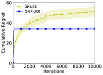
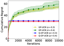
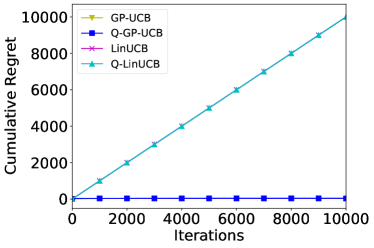
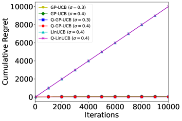
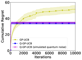
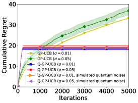
Synthetic Experiment. Here we use a grid of $|\mathcal{X}|=20$ equally spaced points within $[0,1]$ as the $1$-dimensional input domain $\mathcal{X}$ ($d=1$), and sample a function $f$ from a GP prior with the SE kernel. The sampled function $f$ is scaled so that its output is bounded within $[0,1]$, and then used as the reward function in the synthetic experiments. We consider two types of noises: (a) bounded noise (within $[0,1]$) and (b) Gaussian noise, which correspond to the two types of noises in Lemma 1, respectively. For (a) bounded noise, we follow the practice of [38] such that when an input $x$ is selected, we treat the function value $f(x)$ as the probability for a Bernoulli distribution, i.e., we observe an output of $1$ with probability of $f(x)$ and 00 otherwise. For (b) Gaussian noise, we simply add a zero-mean Gaussian noise with variance $\sigma^{2}$ to $f(x)$. The results for (a) bounded noise and (b) Gaussian noise are shown in Figs.Β 1 (a) and (b), respectively. The figures show that for both types of noises, our Q-GP-UCB significantly outperforms the classical baseline of GP-UCB. Specifically, although our Q-GP-UCB incurs larger regrets in the initial stage, it is able to leverage the accurate observations provided by the QMC subroutine to rapidly find the global optimum. These results show that the quantum speedup of our Q-GP-UCB in terms of the tighter regret upper bounds (TheoremsΒ 4 and 5) may also be relevant in practice. We have additionally compared with linear UCB (LinUCB) [2] and Q-LinUCB [38], which are, respectively, the most representative classical and quantum linear bandit algorithms. The results in Fig.Β 2 (App.Β J) show that in these experiments where the reward function is non-linear, algorithms based on linear bandits severely underperform compared with BO/kernelized bandit algorithms in both the classical and quantum settings.

Refer to caption Refer to caption Refer to caption Refer to caption
(a) synthetic (Bernoulli) (b) synthetic (Gaussian) (c) AutoML (d) AutoML
Figure 1: Cumulative regret for synthetic experiments with (a) bounded noise and (b) Gaussian noise. (c) Cumulative regret for the AutoML experiment; (d) additionally includes results for linear bandits.

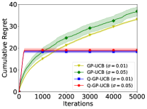
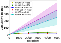
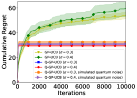
AutoML Experiment. In our experiments on automated machine learning (AutoML), we use our Q-GP-UCB algorithm to tune the hyperparameters of an SVM for a classification task. Here we consider a Gaussian noise with a variance of $\sigma^{2}$ since it is more practical and more commonly used in real-world experiments. The results in Fig.Β 1 (c) show that our Q-GP-UCB again significantly outperforms the classical GP-UCB. Fig.Β 1 (d) additionally shows the comparisons with LinUCB and Q-LinUCB. The results again corroborate that BO/kernelized bandit algorithms are considerably superior in real-world applications with highly non-linear reward functions in both the classical and quantum settings. These results here further demonstrate the potential of our Q-GP-UCB to lead to quantum speedup in practical applications.

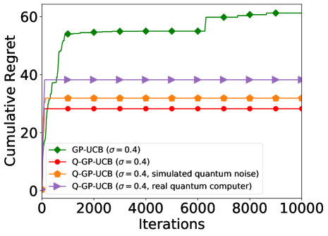
More Realistic Experiments. We have additionally tested the performance of our Q-GP-UCB algorithm after accounting for the effect of quantum noise, by incorporating into our Qiskit simulations a noise model based on the actual performance of real IBM quantum computers. The results (Fig.Β 3 in App.Β J) show that although the addition of quantum noise slightly deteriorates the performance of our Q-GP-UCB, it is still able to significantly outperform classical GP-UCB. Notably, we have additionally performed an experiment using a real quantum computer (details in App.Β J), in which the performance of our Q-GP-UCB, although further worsened compared to the experiment using simulated noise, is still considerably better than classical GP-UCB (Fig.Β 4, App.Β J). Also note that the work of [38] has not shown that Q-LinUCB outperforms LinUCB in the presence of simulated quantum noise. Therefore, the consistently superior performances of our Q-GP-UCB over GP-UCB with both simulated quantum noise and a real quantum computer serve as important new support for the potential practical advantages of quantum bandit algorithms.

Discussion. In our experimental results (e.g., Fig.Β 1), our Q-GP-UCB usually has relatively larger regrets in the initial stages but quickly achieves zero regret thereafter (i.e., the curve plateaus), which has also been observed in [38] for the Q-LinUCB algorithm. This is because in the initial stages, our Q-GP-UCB explores a smaller number of unique arms than GP-UCB. However, after the initial exploration, our Q-GP-UCB quickly starts to perform reliable exploitation, because the accurate reward observations achieved thanks to our QMC subroutines allow us to rapidly learn the reward function and hence find the optimal arm.

7 Conclusion

We have introduced the first quantum BO algorithm, named Q-GP-UCB. Our Q-GP-UCB achieves a regret upper bound of $\mathcal{O}(\text{poly}\log T)$, which is significantly smaller than the classical regret lower bound of $\Omega(\sqrt{T})$. A limitation of our work is that the regret upper bound of our Q-GP-UCB: $\mathcal{O}((\log T)^{3(d+1)/2})$ (ignoring polylog factors) has a worse dependency on the input dimension $d$ than the regret of the classical GP-UCB: $\mathcal{O}((\log T)^{d+1}\sqrt{T})$. A similar limitation is shared by Q-LinUCB, since its regret has a dependency of $\mathcal{O}(d^{3/2})$ in contrast to the $\mathcal{O}(d)$ of LinUCB. It is an interesting future work to explore potential approaches to remove this extra dependency on $d$. Another limitation of our work is that for the MatΓ©rn kernel, we require the reward function to be smooth enough in order to achieve a sub-linear regret upper bound (Sec.Β 5.7). So, another important future work is to further tighten the regret upper bound of our Q-GP-UCB for the MatΓ©rn kernel when the reward function is less smooth, as well as for other kernels encompassing non-smooth functions such as the neural tangent kernel which has been adopted by recent works on neural bandits [13, 42, 44]. Moreover, another interesting future work is to derive regret lower bounds in our setting of quantum kernelized bandits, which can help evaluate the tightness of our regret upper bounds.

Acknowledgements and Disclosure Funding

This research/project is supported by the National Research Foundation, Singapore under its AI Singapore Programme (AISG Award No: AISG-PhD/$2023$-$01$-$039$J). DesCartes: this research is supported by the National Research Foundation, Prime Minister’s Office, Singapore under its Campus for Research Excellence and Technological Enterprise (CREATE) programme.

References

  • [1] A.Β Abbas, D.Β Sutter, C.Β Zoufal, A.Β Lucchi, A.Β Figalli, and S.Β Woerner. The power of quantum neural networks. Nature Computational Science, 1(6):403–409, 2021.
  • [2] Y.Β Abbasi-Yadkori, D.Β PΓ‘l, and C.Β SzepesvΓ‘ri. Improved algorithms for linear stochastic bandits. In Proc. NeurIPS, volumeΒ 24, 2011.
  • [3] J.Β Biamonte, P.Β Wittek, N.Β Pancotti, P.Β Rebentrost, N.Β Wiebe, and S.Β Lloyd. Quantum machine learning. Nature, 549(7671):195–202, 2017.
  • [4] G.Β Brassard, P.Β Hoyer, M.Β Mosca, and A.Β Tapp. Quantum amplitude amplification and estimation. Contemporary Mathematics, 305:53–74, 2002.
  • [5] S.Β Cakmak, R.Β AstudilloΒ Marban, P.Β Frazier, and E.Β Zhou. Bayesian optimization of risk measures. In Proc. NeurIPS, volumeΒ 33, pages 20130–20141, 2020.
  • [6] D.Β Calandriello, L.Β Carratino, A.Β Lazaric, M.Β Valko, and L.Β Rosasco. Scaling Gaussian process optimization by evaluating a few unique candidates multiple times. In Proc. ICML, pages 2523–2541. PMLR, 2022.
  • [7] R.Β Camilleri, K.Β Jamieson, and J.Β Katz-Samuels. High-dimensional experimental design and kernel bandits. In Proc. ICML, pages 1227–1237. PMLR, 2021.
  • [8] B.Β CasalΓ©, G.Β DiΒ Molfetta, H.Β Kadri, and L.Β Ralaivola. Quantum bandits. Quantum Machine Intelligence, 2:1–7, 2020.
  • [9] S.Β R. Chowdhury and A.Β Gopalan. On kernelized multi-armed bandits. In Proc. ICML, pages 844–853, 2017.
  • [10] Z.Β Dai, B.Β K.Β H. Low, and P.Β Jaillet. Federated Bayesian optimization via Thompson sampling. In Proc. NeurIPS, 2020.
  • [11] Z.Β Dai, B.Β K.Β H. Low, and P.Β Jaillet. Differentially private federated Bayesian optimization with distributed exploration. In Proc. NeurIPS, volumeΒ 34, 2021.
  • [12] Z.Β Dai, Y.Β Shu, B.Β K.Β H. Low, and P.Β Jaillet. Sample-then-optimize batch neural Thompson sampling. In Proc. NeurIPS, 2022.
  • [13] Z.Β Dai, Y.Β Shu, A.Β Verma, F.Β X. Fan, B.Β K.Β H. Low, and P.Β Jaillet. Federated neural bandits. In Proc. ICLR, 2023.
  • [14] Z.Β Dai, H.Β Yu, B.Β K.Β H. Low, and P.Β Jaillet. Bayesian optimization meets Bayesian optimal stopping. In Proc. ICML, pages 1496–1506, 2019.
  • [15] Y.Β Deng, X.Β Zhou, B.Β Kim, A.Β Tewari, A.Β Gupta, and N.Β Shroff. Weighted Gaussian process bandits for non-stationary environments. In Proc. AISTATS, pages 6909–6932. PMLR, 2022.
  • [16] P.Β I. Frazier. A tutorial on Bayesian optimization. arXiv preprint arXiv:1807.02811, 2018.
  • [17] B.Β Ganguly, Y.Β Wu, D.Β Wang, and V.Β Aggarwal. Quantum computing provides exponential regret improvement in episodic reinforcement learning. arXiv:2302.08617, 2023.
  • [18] S.Β Garg and G.Β Ramakrishnan. Advances in quantum deep learning: An overview. arXiv preprint arXiv:2005.04316, 2020.
  • [19] R.Β Garnett. Bayesian Optimization. Cambridge Univ. Press, 2022.
  • [20] D.Β Grinko, J.Β Gacon, C.Β Zoufal, and S.Β Woerner. Iterative quantum amplitude estimation. npj Quantum Information, 7(1):52, 2021.
  • [21] L.Β K. Grover. A framework for fast quantum mechanical algorithms. In Proceedings of the thirtieth annual ACM symposium on Theory of computing, pages 53–62, 1998.
  • [22] F.Β Hutter, L.Β Kotthoff, and J.Β Vanschoren. Automated machine learning: methods, systems, challenges. Springer Nature, 2019.
  • [23] T.Β Li and R.Β Zhang. Quantum speedups of optimizing approximately convex functions with applications to logarithmic regret stochastic convex bandits. In Proc. NeurIPS, 2022.
  • [24] Z.Β Li and J.Β Scarlett. Gaussian process bandit optimization with few batches. In Proc. AISTATS, pages 92–107. PMLR, 2022.
  • [25] J.Β Lumbreras, E.Β Haapasalo, and M.Β Tomamichel. Multi-armed quantum bandits: Exploration versus exploitation when learning properties of quantum states. Quantum, 6:749, 2022.
  • [26] A.Β Messiah. Quantum mechanics. Courier Corporation, 2014.
  • [27] N.Β Meyer, C.Β Ufrecht, M.Β Periyasamy, D.Β D. Scherer, A.Β Plinge, and C.Β Mutschler. A survey on quantum reinforcement learning. arXiv:2211.03464, 2022.
  • [28] A.Β Montanaro. Quantum speedup of Monte Carlo methods. Proceedings of the Royal Society A: Mathematical, Physical and Engineering Sciences, 471(2181):20150301, 2015.
  • [29] P.Β Rebentrost, M.Β Mohseni, and S.Β Lloyd. Quantum support vector machine for big data classification. Physical review letters, 113(13):130503, 2014.
  • [30] S.Β Salgia, S.Β Vakili, and Q.Β Zhao. A domain-shrinking based Bayesian optimization algorithm with order-optimal regret performance. In Proc. NeurIPS, volumeΒ 34, pages 28836–28847, 2021.
  • [31] J.Β Scarlett, I.Β Bogunovic, and V.Β Cevher. Lower bounds on regret for noisy Gaussian process bandit optimization. In Proc. COLT, pages 1723–1742. PMLR, 2017.
  • [32] B.Β Shahriari, K.Β Swersky, Z.Β Wang, R.Β P. Adams, and N.Β de Freitas. Taking the human out of the loop: A review of Bayesian optimization. Proceedings of the IEEE, 104(1):148–175, 2016.
  • [33] N.Β Srinivas, A.Β Krause, S.Β M. Kakade, and M.Β Seeger. Gaussian process optimization in the bandit setting: No regret and experimental design. In Proc. ICML, pages 1015–1022, 2010.
  • [34] A.Β Steane. Quantum computing. Reports on Progress in Physics, 61(2):117, 1998.
  • [35] S.Β Vakili, K.Β Khezeli, and V.Β Picheny. On information gain and regret bounds in Gaussian process bandits. In Proc. AISTATS, pages 82–90. PMLR, 2021.
  • [36] M.Β Valko, N.Β Korda, R.Β Munos, I.Β Flaounas, and N.Β Cristianini. Finite-time analysis of kernelised contextual bandits. In Proc. UAI, 2013.
  • [37] A.Β Verma, Z.Β Dai, and B.Β K.Β H. Low. Bayesian optimization under stochastic delayed feedback. In Proc. ICML, pages 22145–22167. PMLR, 2022.
  • [38] Z.Β Wan, Z.Β Zhang, T.Β Li, J.Β Zhang, and X.Β Sun. Quantum multi-armed bandits and stochastic linear bandits enjoy logarithmic regrets. In Proc. AAAI.
  • [39] D.Β Wang, A.Β Sundaram, R.Β Kothari, A.Β Kapoor, and M.Β Roetteler. Quantum algorithms for reinforcement learning with a generative model. In Proc. ICML, pages 10916–10926. PMLR, 2021.
  • [40] D.Β Wang, X.Β You, T.Β Li, and A.Β M. Childs. Quantum exploration algorithms for multi-armed bandits. In Proc. AAAI, volumeΒ 35, pages 10102–10110, 2021.
  • [41] Y.Β Wu, C.Β Guan, V.Β Aggarwal, and D.Β Wang. Quantum heavy-tailed bandits. arXiv:2301.09680, 2023.
  • [42] W.Β Zhang, D.Β Zhou, L.Β Li, and Q.Β Gu. Neural Thompson sampling. In Proc. ICLR, 2021.
  • [43] H.Β Zhong, J.Β Hu, Y.Β Xue, T.Β Li, and L.Β Wang. Provably efficient exploration in quantum reinforcement learning with logarithmic worst-case regret. arXiv:2302.10796, 2023.
  • [44] D.Β Zhou, L.Β Li, and Q.Β Gu. Neural contextual bandits with UCB-based exploration. In Proc. ICML, pages 11492–11502. PMLR, 2020.

Appendix A Analysis of the Weighted GP Posterior (3)

Here we show an alternative view of the weighted GP posterior distribution (3) in the RKHS feature space. The notations in this section will be extensively used in the theoretical analyses in the subsequent sections.

We denote the kernel $k$ by $k(x,x^{\prime})=\phi(x)^{\top}\phi(x^{\prime})$, in which $\phi(x)$ is the potentially infinite-dimensional feature mapping of $x$ in the RKHS of $k$. Define $\Phi_{s}\triangleq[\phi(x_{1}),\ldots,\phi(x_{s})]^{\top}$ which is an sΓ—βˆžπ‘ s\times\infty matrix. Recall that we have defined Wsβ‰œdiag​(1Ο΅12,…,1Ο΅s2)β‰œsubscriptπ‘Šπ‘ diag1superscriptsubscriptitalic-Ο΅12…1superscriptsubscriptitalic-ϡ𝑠2W_{s}\triangleq\text{diag}(\frac{1}{\epsilon_{1}^{2}},\ldots,\frac{1}{\epsilon_{s}^{2}}) which is an $s\times s$ diagonal matrix. Define Vsβ‰œΞ»β€‹I+βˆ‘Ο„=1s1ϡτ2​ϕ​(xΟ„)​ϕ​(xΟ„)⊀=λ​I+Ξ¦sβŠ€β€‹Ws​Φsβ‰œsubscriptπ‘‰π‘ πœ†πΌsubscriptsuperscriptπ‘ πœ11superscriptsubscriptitalic-ϡ𝜏2italic-Ο•subscriptπ‘₯𝜏italic-Ο•superscriptsubscriptπ‘₯𝜏topπœ†πΌsuperscriptsubscriptΦ𝑠topsubscriptπ‘Šπ‘ subscriptΦ𝑠V_{s}\triangleq\lambda I+\sum^{s}_{\tau=1}\frac{1}{\epsilon_{\tau}^{2}}\phi(x_{\tau})\phi(x_{\tau})^{\top}=\lambda I+\Phi_{s}^{\top}W_{s}\Phi_{s} which is an $\infty\times\infty$ matrix, and let $V_{0}\triangleq\lambda I$. With these notations, it can be easily verified that $K_{s}=\Phi_{s}\Phi_{s}^{\top}=[k(x_{\tau},x_{\tau^{\prime}})]_{\tau,\tau^{\prime}=1,\ldots,s}$, and K~s=Ws1/2​Φs​ΦsβŠ€β€‹Ws1/2=Ws1/2​Ks​Ws1/2subscript~𝐾𝑠superscriptsubscriptπ‘Šπ‘ 12subscriptΦ𝑠superscriptsubscriptΦ𝑠topsuperscriptsubscriptπ‘Šπ‘ 12superscriptsubscriptπ‘Šπ‘ 12subscript𝐾𝑠superscriptsubscriptπ‘Šπ‘ 12\widetilde{K}_{s}=W_{s}^{1/2}\Phi_{s}\Phi_{s}^{\top}W_{s}^{1/2}=W_{s}^{1/2}K_{s}W_{s}^{1/2}. Moreover, we can also easily show that ks​(x)=Ξ¦s​ϕ​(x)=[k​(x,xΟ„)]Ο„=1,…,ssubscriptπ‘˜π‘ π‘₯subscriptΦ𝑠italic-Ο•π‘₯subscriptdelimited-[]π‘˜π‘₯subscriptπ‘₯𝜏𝜏1…𝑠k_{s}(x)=\Phi_{s}\phi(x)=[k(x,x_{\tau})]_{\tau=1,\ldots,s}, k~s​(x)=Ws1/2​Φs​ϕ​(x)=Ws1/2​ks​(x)subscript~π‘˜π‘ π‘₯superscriptsubscriptπ‘Šπ‘ 12subscriptΦ𝑠italic-Ο•π‘₯superscriptsubscriptπ‘Šπ‘ 12subscriptπ‘˜π‘ π‘₯\widetilde{k}_{s}(x)=W_{s}^{1/2}\Phi_{s}\phi(x)=W_{s}^{1/2}k_{s}(x), and Y~s=Ws1/2​Yssubscript~π‘Œπ‘ superscriptsubscriptπ‘Šπ‘ 12subscriptπ‘Œπ‘ \widetilde{Y}_{s}=W_{s}^{1/2}Y_{s}.

We start by deriving an alternative expression for the weighted GP posterior mean ΞΌ~s​(x)subscript~πœ‡π‘ π‘₯\widetilde{\mu}_{s}(x). To begin with, we have that

Ξ¦sβŠ€β€‹Ws1/2​(K~s+λ​I)=Ξ¦sβŠ€β€‹Ws1/2​(Ws1/2​Φs​ΦsβŠ€β€‹Ws1/2+λ​I)=Ξ¦sβŠ€β€‹Ws1/2​Ws1/2​Φs​ΦsβŠ€β€‹Ws1/2+λ​ΦsβŠ€β€‹Ws1/2=(Ξ¦sβŠ€β€‹Ws​Φs+λ​I)​ΦsβŠ€β€‹Ws1/2=Vs​ΦsβŠ€β€‹Ws1/2.superscriptsubscriptΦ𝑠topsuperscriptsubscriptπ‘Šπ‘ 12subscript~πΎπ‘ πœ†πΌsuperscriptsubscriptΦ𝑠topsuperscriptsubscriptπ‘Šπ‘ 12superscriptsubscriptπ‘Šπ‘ 12subscriptΦ𝑠superscriptsubscriptΦ𝑠topsuperscriptsubscriptπ‘Šπ‘ 12πœ†πΌsuperscriptsubscriptΦ𝑠topsuperscriptsubscriptπ‘Šπ‘ 12superscriptsubscriptπ‘Šπ‘ 12subscriptΦ𝑠superscriptsubscriptΦ𝑠topsuperscriptsubscriptπ‘Šπ‘ 12πœ†superscriptsubscriptΦ𝑠topsuperscriptsubscriptπ‘Šπ‘ 12superscriptsubscriptΦ𝑠topsubscriptπ‘Šπ‘ subscriptΞ¦π‘ πœ†πΌsuperscriptsubscriptΦ𝑠topsuperscriptsubscriptπ‘Šπ‘ 12subscript𝑉𝑠superscriptsubscriptΦ𝑠topsuperscriptsubscriptπ‘Šπ‘ 12\begin{split}\Phi_{s}^{\top}W_{s}^{1/2}(\widetilde{K}_{s}+\lambda I)&=\Phi_{s}^{\top}W_{s}^{1/2}(W_{s}^{1/2}\Phi_{s}\Phi_{s}^{\top}W_{s}^{1/2}+\lambda I)\\ &=\Phi_{s}^{\top}W_{s}^{1/2}W_{s}^{1/2}\Phi_{s}\Phi_{s}^{\top}W_{s}^{1/2}+\lambda\Phi_{s}^{\top}W_{s}^{1/2}\\ &=(\Phi_{s}^{\top}W_{s}\Phi_{s}+\lambda I)\Phi_{s}^{\top}W_{s}^{1/2}\\ &=V_{s}\Phi_{s}^{\top}W_{s}^{1/2}.\end{split}

Now we multiply both sides by $V_{s}^{-1}$ on the left and by (K~s+λ​I)βˆ’1superscriptsubscript~πΎπ‘ πœ†πΌ1(\widetilde{K}_{s}+\lambda I)^{-1} on the right, which leads to

Vsβˆ’1​ΦsβŠ€β€‹Ws1/2=Ξ¦sβŠ€β€‹Ws1/2​(K~s+λ​I)βˆ’1superscriptsubscript𝑉𝑠1superscriptsubscriptΦ𝑠topsuperscriptsubscriptπ‘Šπ‘ 12superscriptsubscriptΦ𝑠topsuperscriptsubscriptπ‘Šπ‘ 12superscriptsubscript~πΎπ‘ πœ†πΌ1\begin{split}V_{s}^{-1}\Phi_{s}^{\top}W_{s}^{1/2}=\Phi_{s}^{\top}W_{s}^{1/2}(\widetilde{K}_{s}+\lambda I)^{-1}\end{split}

Now we can show that

ΞΌ~s​(x)=ϕ​(x)βŠ€β€‹Vsβˆ’1​ΦsβŠ€β€‹Ws​Ys=ϕ​(x)βŠ€β€‹Ξ¦sβŠ€β€‹Ws1/2​(K~s+λ​I)βˆ’1​Ws1/2​Ys=k~sβŠ€β€‹(x)​(K~s+λ​I)βˆ’1​Y~s.subscript~πœ‡π‘ π‘₯italic-Ο•superscriptπ‘₯topsuperscriptsubscript𝑉𝑠1superscriptsubscriptΦ𝑠topsubscriptπ‘Šπ‘ subscriptπ‘Œπ‘ italic-Ο•superscriptπ‘₯topsuperscriptsubscriptΦ𝑠topsuperscriptsubscriptπ‘Šπ‘ 12superscriptsubscript~πΎπ‘ πœ†πΌ1superscriptsubscriptπ‘Šπ‘ 12subscriptπ‘Œπ‘ subscriptsuperscript~π‘˜top𝑠π‘₯superscriptsubscript~πΎπ‘ πœ†πΌ1subscript~π‘Œπ‘ \begin{split}\widetilde{\mu}_{s}(x)=\phi(x)^{\top}V_{s}^{-1}\Phi_{s}^{\top}W_{s}Y_{s}&=\phi(x)^{\top}\Phi_{s}^{\top}W_{s}^{1/2}(\widetilde{K}_{s}+\lambda I)^{-1}W_{s}^{1/2}Y_{s}\\ &=\widetilde{k}^{\top}_{s}(x)(\widetilde{K}_{s}+\lambda I)^{-1}\widetilde{Y}_{s}.\end{split}

Next, we derive an alternative expression for the weighted GP posterior variance $\widetilde{\sigma}^{2}_{s}(x)$. To begin with, we have that

(Wsβˆ’1+1λ​Φs​Φs⊀)βˆ’1=(Wsβˆ’1/2​(I+1λ​Ws1/2​Φs​ΦsβŠ€β€‹Ws1/2)​Wsβˆ’1/2)βˆ’1=Ws1/2​(I+1λ​Ws1/2​Φs​ΦsβŠ€β€‹Ws1/2)βˆ’1​Ws1/2=λ​Ws1/2​(λ​I+K~s)βˆ’1​Ws1/2.superscriptsuperscriptsubscriptπ‘Šπ‘ 11πœ†subscriptΦ𝑠superscriptsubscriptΦ𝑠top1superscriptsuperscriptsubscriptπ‘Šπ‘ 12𝐼1πœ†superscriptsubscriptπ‘Šπ‘ 12subscriptΦ𝑠superscriptsubscriptΦ𝑠topsuperscriptsubscriptπ‘Šπ‘ 12superscriptsubscriptπ‘Šπ‘ 121superscriptsubscriptπ‘Šπ‘ 12superscript𝐼1πœ†superscriptsubscriptπ‘Šπ‘ 12subscriptΦ𝑠superscriptsubscriptΦ𝑠topsuperscriptsubscriptπ‘Šπ‘ 121superscriptsubscriptπ‘Šπ‘ 12πœ†superscriptsubscriptπ‘Šπ‘ 12superscriptπœ†πΌsubscript~𝐾𝑠1superscriptsubscriptπ‘Šπ‘ 12\begin{split}\left(W_{s}^{-1}+\frac{1}{\lambda}\Phi_{s}\Phi_{s}^{\top}\right)^{-1}&=\left(W_{s}^{-1/2}\left(I+\frac{1}{\lambda}W_{s}^{1/2}\Phi_{s}\Phi_{s}^{\top}W_{s}^{1/2}\right)W_{s}^{-1/2}\right)^{-1}\\ &=W_{s}^{1/2}\left(I+\frac{1}{\lambda}W_{s}^{1/2}\Phi_{s}\Phi_{s}^{\top}W_{s}^{1/2}\right)^{-1}W_{s}^{1/2}\\ &=\lambda W_{s}^{1/2}\left(\lambda I+\widetilde{K}_{s}\right)^{-1}W_{s}^{1/2}.\end{split} (5)

This allows us to show that

Οƒ~s2​(x)=λ​ϕ​(x)βŠ€β€‹Vsβˆ’1​ϕ​(x)=λ​ϕ​(x)βŠ€β€‹(λ​I+Ξ¦sβŠ€β€‹Ws​Φs)βˆ’1​ϕ​(x)=(a)λ​ϕ​(x)βŠ€β€‹(1λ​Iβˆ’1λ​ΦsβŠ€β€‹(Wsβˆ’1+Ξ¦s​1λ​Φs⊀)βˆ’1​Φs​1Ξ»)​ϕ​(x)=ϕ​(x)βŠ€β€‹Ο•β€‹(x)βˆ’Ο•β€‹(x)βŠ€β€‹Ξ¦sβŠ€β€‹(Wsβˆ’1+1λ​Φs​Φs⊀)βˆ’1​Φs​1λ​ϕ​(x)=(b)ϕ​(x)βŠ€β€‹Ο•β€‹(x)βˆ’Ο•β€‹(x)βŠ€β€‹Ξ¦sβŠ€β€‹Ws1/2​(λ​I+K~s)βˆ’1​Ws1/2​Φs​ϕ​(x)=k​(x,x)βˆ’k~sβŠ€β€‹(x)​(K~s+λ​I)βˆ’1​k~s​(x),subscriptsuperscript~𝜎2𝑠π‘₯πœ†italic-Ο•superscriptπ‘₯topsuperscriptsubscript𝑉𝑠1italic-Ο•π‘₯πœ†italic-Ο•superscriptπ‘₯topsuperscriptπœ†πΌsuperscriptsubscriptΦ𝑠topsubscriptπ‘Šπ‘ subscriptΦ𝑠1italic-Ο•π‘₯superscriptπ‘Žπœ†italic-Ο•superscriptπ‘₯top1πœ†πΌ1πœ†superscriptsubscriptΦ𝑠topsuperscriptsuperscriptsubscriptπ‘Šπ‘ 1subscriptΦ𝑠1πœ†superscriptsubscriptΦ𝑠top1subscriptΦ𝑠1πœ†italic-Ο•π‘₯italic-Ο•superscriptπ‘₯topitalic-Ο•π‘₯italic-Ο•superscriptπ‘₯topsuperscriptsubscriptΦ𝑠topsuperscriptsuperscriptsubscriptπ‘Šπ‘ 11πœ†subscriptΦ𝑠superscriptsubscriptΦ𝑠top1subscriptΦ𝑠1πœ†italic-Ο•π‘₯superscript𝑏italic-Ο•superscriptπ‘₯topitalic-Ο•π‘₯italic-Ο•superscriptπ‘₯topsuperscriptsubscriptΦ𝑠topsuperscriptsubscriptπ‘Šπ‘ 12superscriptπœ†πΌsubscript~𝐾𝑠1superscriptsubscriptπ‘Šπ‘ 12subscriptΦ𝑠italic-Ο•π‘₯π‘˜π‘₯π‘₯superscriptsubscript~π‘˜π‘ topπ‘₯superscriptsubscript~πΎπ‘ πœ†πΌ1subscript~π‘˜π‘ π‘₯\begin{split}\widetilde{\sigma}^{2}_{s}(x)&=\lambda\phi(x)^{\top}V_{s}^{-1}\phi(x)\\ &=\lambda\phi(x)^{\top}(\lambda I+\Phi_{s}^{\top}W_{s}\Phi_{s})^{-1}\phi(x)\\ &\stackrel{{\scriptstyle(a)}}{{=}}\lambda\phi(x)^{\top}\left(\frac{1}{\lambda}I-\frac{1}{\lambda}\Phi_{s}^{\top}(W_{s}^{-1}+\Phi_{s}\frac{1}{\lambda}\Phi_{s}^{\top})^{-1}\Phi_{s}\frac{1}{\lambda}\right)\phi(x)\\ &=\phi(x)^{\top}\phi(x)-\phi(x)^{\top}\Phi_{s}^{\top}(W_{s}^{-1}+\frac{1}{\lambda}\Phi_{s}\Phi_{s}^{\top})^{-1}\Phi_{s}\frac{1}{\lambda}\phi(x)\\ &\stackrel{{\scriptstyle(b)}}{{=}}\phi(x)^{\top}\phi(x)-\phi(x)^{\top}\Phi_{s}^{\top}W_{s}^{1/2}\left(\lambda I+\widetilde{K}_{s}\right)^{-1}W_{s}^{1/2}\Phi_{s}\phi(x)\\ &=k(x,x)-\widetilde{k}_{s}^{\top}(x)(\widetilde{K}_{s}+\lambda I)^{-1}\widetilde{k}_{s}(x),\end{split}

in which we have used the matrix inversion lemma in step $(a)$, and used equation (5) in step $(b)$.

To summarize, we have derived the following alternative expressions for the weighted GP posterior distribution (3):

ΞΌ~s​(x)=ϕ​(x)βŠ€β€‹Vsβˆ’1​ΦsβŠ€β€‹Ws​Ys=k~sβŠ€β€‹(x)​(K~s+λ​I)βˆ’1​Y~s,Οƒ~s2​(x)=λ​ϕ​(x)βŠ€β€‹Vsβˆ’1​ϕ​(x)=k​(x,x)βˆ’k~sβŠ€β€‹(x)​(K~s+λ​I)βˆ’1​k~s​(x).formulae-sequencesubscript~πœ‡π‘ π‘₯italic-Ο•superscriptπ‘₯topsuperscriptsubscript𝑉𝑠1superscriptsubscriptΦ𝑠topsubscriptπ‘Šπ‘ subscriptπ‘Œπ‘ superscriptsubscript~π‘˜π‘ topπ‘₯superscriptsubscript~πΎπ‘ πœ†πΌ1subscript~π‘Œπ‘ subscriptsuperscript~𝜎2𝑠π‘₯πœ†italic-Ο•superscriptπ‘₯topsuperscriptsubscript𝑉𝑠1italic-Ο•π‘₯π‘˜π‘₯π‘₯superscriptsubscript~π‘˜π‘ topπ‘₯superscriptsubscript~πΎπ‘ πœ†πΌ1subscript~π‘˜π‘ π‘₯\begin{split}\widetilde{\mu}_{s}(x)&=\phi(x)^{\top}V_{s}^{-1}\Phi_{s}^{\top}W_{s}Y_{s}=\widetilde{k}_{s}^{\top}(x)(\widetilde{K}_{s}+\lambda I)^{-1}\widetilde{Y}_{s},\\ \widetilde{\sigma}^{2}_{s}(x)&=\lambda\phi(x)^{\top}V_{s}^{-1}\phi(x)=k(x,x)-\widetilde{k}_{s}^{\top}(x)(\widetilde{K}_{s}+\lambda I)^{-1}\widetilde{k}_{s}(x).\end{split} (6)

Appendix B Proof of Lemma 2

To begin with, we can lower-bound the total number of iterations (i.e., the total number of queries to the quantum oracles) in $m$ stages by

βˆ‘s=1mC1Ο΅s​log⁑(2​mΒ―Ξ΄)β‰₯βˆ‘s=1m1Ο΅sβ‰₯βˆ‘s=1m1Ο΅s2.subscriptsuperscriptπ‘šπ‘ 1subscript𝐢1subscriptitalic-ϡ𝑠2Β―π‘šπ›Ώsubscriptsuperscriptπ‘šπ‘ 11subscriptitalic-ϡ𝑠subscriptsuperscriptπ‘šπ‘ 11superscriptsubscriptitalic-ϡ𝑠2\sum^{m}_{s=1}\frac{C_{1}}{\epsilon_{s}}\log(\frac{2\overline{m}}{\delta})\geq\sum^{m}_{s=1}\frac{1}{\epsilon_{s}}\geq\sqrt{\sum^{m}_{s=1}\frac{1}{\epsilon_{s}^{2}}}. (7)

The first inequality follows since $C_{1}>1$ (Lemma 1) and $\log(\frac{2\overline{m}}{\delta})\geq\log(\frac{2}{\delta})\geq 1$ because we have chosen $\delta\in(0,2/e]$. Suppose that βˆ‘s=1m1Ο΅s2>T2subscriptsuperscriptπ‘šπ‘ 11superscriptsubscriptitalic-ϡ𝑠2superscript𝑇2\sum^{m}_{s=1}\frac{1}{\epsilon_{s}^{2}}>T^{2}, then we have that βˆ‘s=1mC1Ο΅s​log⁑(2​mΒ―Ξ΄)>Tsubscriptsuperscriptπ‘šπ‘ 1subscript𝐢1subscriptitalic-ϡ𝑠2Β―π‘šπ›Ώπ‘‡\sum^{m}_{s=1}\frac{C_{1}}{\epsilon_{s}}\log(\frac{2\overline{m}}{\delta})>T which is a contradiction. Therefore, we have that

βˆ‘s=1m1Ο΅s2≀T2.subscriptsuperscriptπ‘šπ‘ 11superscriptsubscriptitalic-ϡ𝑠2superscript𝑇2\sum^{m}_{s=1}\frac{1}{\epsilon_{s}^{2}}\leq T^{2}. (8)

Appendix C Proof of Theorem 1

Here we prove the growth rate of $\widetilde{\gamma}_{m}$, i.e., the weighted information gain. Recall that $W_{m}=\text{diag}\left(\frac{1}{\epsilon_{1}^{2}},\frac{1}{\epsilon_{2}^{2}},\ldots,\frac{1}{\epsilon_{m}^{2}}\right)$, and $\widetilde{\gamma}_{m}=\frac{1}{2}\log\det\left(I+\lambda^{-1}\widetilde{K}_{m}\right)$. Our proof here follows closely the proof of Theorem 3 from the work of [35]. We will omit the subscript $m$ as long as the context is clear.

Denote by $K_{m}=\Phi_{m}\Phi_{m}^{\top}=[k(x_{i},x_{j})]_{i,j=1,\ldots,m}$ the $m\times m$ covariance matrix, and define $\widetilde{K}_{m}=W_{m}^{1/2}\Phi_{m}\Phi_{m}^{\top}W_{m}^{1/2}=W^{1/2}_{m}K_{m}W^{1/2}_{m}$. Following Theorem 1 from [35], our kernel $k$ can be denoted as $k(x,x^{\prime})=\sum^{\infty}_{\tau=1}\lambda_{\tau}\psi_{\tau}(x)\psi_{\tau}(x^{\prime})$, in which $\{\lambda_{\tau}\}_{\tau=1,\ldots,\infty}$ and $\{\psi_{\tau}\}_{\tau=1,\ldots,\infty}$ represent, respectively, the eigenvalues and eigenfunctions of the kernel $k$. We will make use of the projection onto a $D$-dimensional RKHS ($D<\infty$), which consists of the first $D$ features corresponding to the $D$ largest eigenvalues of the kernel $k$. Specifically, define $k_{P}$ as the $D$-dimensional projection in the RKHS of $k$, and $k_{O}$ corresponds to the orthogonal element such that $k(\cdot,\cdot)=k_{P}(\cdot,\cdot)+k_{O}(\cdot,\cdot)$. That is, following Section 3.2 from the work of [35], define

$$k_{P}(x,x^{\prime})=\sum^{D}_{\tau=1}\lambda_{\tau}\psi_{\tau}(x)\psi_{\tau}(x^{\prime}).$$ (9)

We define $K_{P}\triangleq[k_{P}(x_{i},x_{j})]_{i,j=1,\ldots,m}$ and $K_{O}\triangleq[k_{O}(x_{i},x_{j})]_{i,j=1,\ldots,m}$. Similarly, define $\widetilde{K}_{P}=W^{1/2}_{m}K_{P}W^{1/2}_{m}$ and $\widetilde{K}_{O}=W^{1/2}_{m}K_{O}W^{1/2}_{m}$. This implies that $K_{m}=K_{P}+K_{O}$ and that $\widetilde{K}_{m}=\widetilde{K}_{P}+\widetilde{K}_{O}$.

Here to be consistent with [35], we use $I_{m}$ to denote the $m\times m$-dimensional identity matrix. Denote by $\widetilde{I}(\mathbf{y}_{m};f)$ the information gain about the function $f$ from the observations $\mathbf{y}_{m}=[y_{1},\ldots,y_{m}]$. We have that

$$\begin{split}\widetilde{I}(\mathbf{y}_{m};f)&=\frac{1}{2}\log\det\left(I_{m}+\frac{1}{\lambda}\widetilde{K}_{m}\right)\\ &=\frac{1}{2}\log\det\left(I_{m}+\frac{1}{\lambda}\left(\widetilde{K}_{P}+\widetilde{K}_{O}\right)\right)\\ &=\frac{1}{2}\log\det\left(\left(I_{m}+\frac{1}{\lambda}\widetilde{K}_{P}\right)\left(I_{m}+\frac{1}{\lambda}\left(I_{m}+\frac{1}{\lambda}\widetilde{K}_{P}\right)^{-1}\widetilde{K}_{O}\right)\right)\\ &=\frac{1}{2}\log\det\left(I_{m}+\frac{1}{\lambda}\widetilde{K}_{P}\right)+\frac{1}{2}\log\det\left(I_{m}+\frac{1}{\lambda}\left(I_{m}+\frac{1}{\lambda}\widetilde{K}_{P}\right)^{-1}\widetilde{K}_{O}\right).\end{split}$$ (10)

The last line follows because $\det{(AB)}=\det{(A)}\det{(B)}$. In the following, we will separately upper-bound the two terms in (10).

We start by upper-bounding the first term in equation (10). Denote by $\boldsymbol{\psi}_{D}(x)$ the $D$-dimensional feature vector corresponding to the first $D$ principle features of the kernel $k$ (i.e., the features corresponding to the largest $D$ eigenvalues). Define $\Psi_{m,D}\triangleq[\boldsymbol{\psi}_{D}(x_{1}),\ldots,\boldsymbol{\psi}_{D}(x_{m})]^{\top}$ which is an $m\times D$ matrix. Denote by $\Lambda_{D}=\text{diag}(\lambda_{1},\ldots,\lambda_{D})$ a $D\times D$-diagonal matrix whose diagonal entries consist of the largest $D$ eigenvalues of the kernel $k$ in descending order. With this definition, we have that $K_{P}=\Psi_{m,D}\Lambda_{D}\Psi_{m,D}^{\top}$ and

$$\widetilde{K}_{P}=W^{1/2}_{m}\Psi_{m,D}\Lambda_{D}\Psi_{m,D}^{\top}W^{1/2}_{m}.$$ (11)

Also define the gram matrix:

$$\widetilde{G}_{m}=\Lambda_{D}^{1/2}\Psi_{m,D}^{\top}W_{m}\Psi_{m,D}\Lambda_{D}^{1/2}.$$ (12)

Based on these definitions, we have that

$$\det\left(I_{D}+\frac{1}{\lambda}\widetilde{G}_{m}\right)=\det\left(I_{m}+\frac{1}{\lambda}\widetilde{K}_{P}\right),$$ (13)

which follows from the Weinstein–Aronszajn identity: $\det\left(I_{D}+AA^{\top}\right)=\det\left(I_{m}+A^{\top}A\right)$ for a $D\times m$ matrix $A$, and we have plugged in $A=\frac{1}{\sqrt{\lambda}}\Lambda_{D}^{1/2}\Psi_{m,D}^{\top}W_{m}^{1/2}$. In addition, the following inequality will also be useful in the subsequent proof:

$$\mathinner{\!\left\lVert\Lambda_{D}^{1/2}\boldsymbol{\psi}_{D}(x)\right\rVert}_{2}^{2}=\sum^{D}_{\tau=1}\lambda_{\tau}\psi_{\tau}^{2}(x)=k_{P}(x,x)\leq k(x,x)\leq 1,$$ (14)

in which we have made use of the definition of $k_{P}$ from (9), and our assumption (w.l.o.g.) that $k(x,x^{\prime})\leq 1,\forall x,x^{\prime}$ (Sec.Β 3.1). In the following, we will denote the trace of a matrix $A$ by $\text{Tr}(A)$. Next, we have that

Tr​(ID+1λ​G~m)=D+1λ​Tr​(G~m)=D+1λ​Tr​(Ξ›D1/2​Ψm,DβŠ€β€‹Wm​Ψm,D​ΛD1/2)=(a)D+1λ​Tr​(Ξ›D1/2​[βˆ‘s=1m1Ο΅s2​𝝍D​(xs)​𝝍DβŠ€β€‹(xs)]​ΛD1/2)=D+1λ​Tr​(βˆ‘s=1m1Ο΅s2​ΛD1/2​𝝍D​(xs)​𝝍DβŠ€β€‹(xs)​ΛD1/2)=D+1Ξ»β€‹βˆ‘s=1m1Ο΅s2​Tr​(Ξ›D1/2​𝝍D​(xs)​𝝍DβŠ€β€‹(xs)​ΛD1/2)=(b)D+1Ξ»β€‹βˆ‘s=1m1Ο΅s2​Tr​(𝝍DβŠ€β€‹(xs)​ΛD1/2​ΛD1/2​𝝍D​(xs))=D+1Ξ»β€‹βˆ‘s=1m1Ο΅s2​𝝍DβŠ€β€‹(xs)​ΛD1/2​ΛD1/2​𝝍D​(xs)=D+1Ξ»β€‹βˆ‘s=1m1Ο΅s2​βˆ₯Ξ›D1/2​𝝍D​(xs)βˆ₯22≀(c)D+1Ξ»β€‹βˆ‘s=1m1Ο΅s2,Trsubscript𝐼𝐷1πœ†subscript~πΊπ‘šπ·1πœ†Trsubscript~πΊπ‘šπ·1πœ†TrsuperscriptsubscriptΛ𝐷12superscriptsubscriptΞ¨π‘šπ·topsubscriptπ‘Šπ‘šsubscriptΞ¨π‘šπ·superscriptsubscriptΛ𝐷12superscriptπ‘Žπ·1πœ†TrsuperscriptsubscriptΛ𝐷12delimited-[]subscriptsuperscriptπ‘šπ‘ 11superscriptsubscriptitalic-ϡ𝑠2subscript𝝍𝐷subscriptπ‘₯𝑠superscriptsubscript𝝍𝐷topsubscriptπ‘₯𝑠superscriptsubscriptΛ𝐷12𝐷1πœ†Trsubscriptsuperscriptπ‘šπ‘ 11superscriptsubscriptitalic-ϡ𝑠2superscriptsubscriptΛ𝐷12subscript𝝍𝐷subscriptπ‘₯𝑠superscriptsubscript𝝍𝐷topsubscriptπ‘₯𝑠superscriptsubscriptΛ𝐷12𝐷1πœ†subscriptsuperscriptπ‘šπ‘ 11superscriptsubscriptitalic-ϡ𝑠2TrsuperscriptsubscriptΛ𝐷12subscript𝝍𝐷subscriptπ‘₯𝑠superscriptsubscript𝝍𝐷topsubscriptπ‘₯𝑠superscriptsubscriptΛ𝐷12superscript𝑏𝐷1πœ†subscriptsuperscriptπ‘šπ‘ 11superscriptsubscriptitalic-ϡ𝑠2Trsuperscriptsubscript𝝍𝐷topsubscriptπ‘₯𝑠superscriptsubscriptΛ𝐷12superscriptsubscriptΛ𝐷12subscript𝝍𝐷subscriptπ‘₯𝑠𝐷1πœ†subscriptsuperscriptπ‘šπ‘ 11superscriptsubscriptitalic-ϡ𝑠2superscriptsubscript𝝍𝐷topsubscriptπ‘₯𝑠superscriptsubscriptΛ𝐷12superscriptsubscriptΛ𝐷12subscript𝝍𝐷subscriptπ‘₯𝑠𝐷1πœ†subscriptsuperscriptπ‘šπ‘ 11superscriptsubscriptitalic-ϡ𝑠2superscriptsubscriptdelimited-βˆ₯βˆ₯superscriptsubscriptΛ𝐷12subscript𝝍𝐷subscriptπ‘₯𝑠22superscript𝑐𝐷1πœ†subscriptsuperscriptπ‘šπ‘ 11superscriptsubscriptitalic-ϡ𝑠2\begin{split}\text{Tr}\left(I_{D}+\frac{1}{\lambda}\widetilde{G}_{m}\right)&=D+\frac{1}{\lambda}\text{Tr}\left(\widetilde{G}_{m}\right)\\ &=D+\frac{1}{\lambda}\text{Tr}\left(\Lambda_{D}^{1/2}\Psi_{m,D}^{\top}W_{m}\Psi_{m,D}\Lambda_{D}^{1/2}\right)\\ &\stackrel{{\scriptstyle(a)}}{{=}}D+\frac{1}{\lambda}\text{Tr}\left(\Lambda_{D}^{1/2}\left[\sum^{m}_{s=1}\frac{1}{\epsilon_{s}^{2}}\boldsymbol{\psi}_{D}(x_{s})\boldsymbol{\psi}_{D}^{\top}(x_{s})\right]\Lambda_{D}^{1/2}\right)\\ &=D+\frac{1}{\lambda}\text{Tr}\left(\sum^{m}_{s=1}\frac{1}{\epsilon_{s}^{2}}\Lambda_{D}^{1/2}\boldsymbol{\psi}_{D}(x_{s})\boldsymbol{\psi}_{D}^{\top}(x_{s})\Lambda_{D}^{1/2}\right)\\ &=D+\frac{1}{\lambda}\sum^{m}_{s=1}\frac{1}{\epsilon_{s}^{2}}\text{Tr}\left(\Lambda_{D}^{1/2}\boldsymbol{\psi}_{D}(x_{s})\boldsymbol{\psi}_{D}^{\top}(x_{s})\Lambda_{D}^{1/2}\right)\\ &\stackrel{{\scriptstyle(b)}}{{=}}D+\frac{1}{\lambda}\sum^{m}_{s=1}\frac{1}{\epsilon_{s}^{2}}\text{Tr}\left(\boldsymbol{\psi}_{D}^{\top}(x_{s})\Lambda_{D}^{1/2}\Lambda_{D}^{1/2}\boldsymbol{\psi}_{D}(x_{s})\right)\\ &=D+\frac{1}{\lambda}\sum^{m}_{s=1}\frac{1}{\epsilon_{s}^{2}}\boldsymbol{\psi}_{D}^{\top}(x_{s})\Lambda_{D}^{1/2}\Lambda_{D}^{1/2}\boldsymbol{\psi}_{D}(x_{s})\\ &=D+\frac{1}{\lambda}\sum^{m}_{s=1}\frac{1}{\epsilon_{s}^{2}}\mathinner{\!\left\lVert\Lambda_{D}^{1/2}\boldsymbol{\psi}_{D}(x_{s})\right\rVert}_{2}^{2}\\ &\stackrel{{\scriptstyle(c)}}{{\leq}}D+\frac{1}{\lambda}\sum^{m}_{s=1}\frac{1}{\epsilon_{s}^{2}},\end{split} (15)

in which $(a)$ follows because Ξ¨m,DβŠ€β€‹Wm​Ψm,D=βˆ‘s=1m1Ο΅s2​𝝍D​(xs)​𝝍DβŠ€β€‹(xs)superscriptsubscriptΞ¨π‘šπ·topsubscriptπ‘Šπ‘šsubscriptΞ¨π‘šπ·subscriptsuperscriptπ‘šπ‘ 11superscriptsubscriptitalic-ϡ𝑠2subscript𝝍𝐷subscriptπ‘₯𝑠superscriptsubscript𝝍𝐷topsubscriptπ‘₯𝑠\Psi_{m,D}^{\top}W_{m}\Psi_{m,D}=\sum^{m}_{s=1}\frac{1}{\epsilon_{s}^{2}}\boldsymbol{\psi}_{D}(x_{s})\boldsymbol{\psi}_{D}^{\top}(x_{s}), $(b)$ has made use of the cyclic property of the trace operator, and $(c)$ follows from (14) above.

Also note that for a positive definite matrix $P\in\mathbb{R}^{n\times n}$, we have that

$$\log\det(P)\leq n\log\frac{\text{Tr}(P)}{n}.$$ (16)

Therefore, we have that

log​det(Im+1λ​K~P)=log​det(ID+1λ​G~m)≀D​log⁑D+1Ξ»β€‹βˆ‘s=1m1Ο΅s2D=D​log⁑(1+1λ​Dβ€‹βˆ‘s=1m1Ο΅s2).subscriptπΌπ‘š1πœ†subscript~𝐾𝑃subscript𝐼𝐷1πœ†subscript~πΊπ‘šπ·π·1πœ†subscriptsuperscriptπ‘šπ‘ 11superscriptsubscriptitalic-ϡ𝑠2𝐷𝐷11πœ†π·subscriptsuperscriptπ‘šπ‘ 11superscriptsubscriptitalic-ϡ𝑠2\begin{split}\log\det\left(I_{m}+\frac{1}{\lambda}\widetilde{K}_{P}\right)&=\log\det\left(I_{D}+\frac{1}{\lambda}\widetilde{G}_{m}\right)\\ &\leq D\log\frac{D+\frac{1}{\lambda}\sum^{m}_{s=1}\frac{1}{\epsilon_{s}^{2}}}{D}=D\log\left(1+\frac{1}{\lambda D}\sum^{m}_{s=1}\frac{1}{\epsilon_{s}^{2}}\right).\end{split} (17)

The first equality follows from (13), and the inequality results from (16) and (15).

Now we upper-bound the second term in equation (10). To begin with, we have that

$$\begin{split}\text{Tr}\left(\left(I_{m}+\frac{1}{\lambda}\widetilde{K}_{P}\right)^{-1}\widetilde{K}_{O}\right)\leq\text{Tr}\left(\widetilde{K}_{O}\right),\end{split}$$ (18)

which is because the matrix $\left(I_{m}+\frac{1}{\lambda}\widetilde{K}_{P}\right)^{-1}$ is positive semi-definite (PSD) whose largest eigenvalue is upper-bounded by $1$, and $\text{Tr}(P_{1}P_{2})\leq\lambda_{P_{1}}\text{Tr}(P_{2})$ where $P_{1}$ and $P_{2}$ are PSD matrices and $\lambda_{P_{1}}$ is the largest eigenvalue of $P_{1}$. Next, define $\delta_{D}\triangleq\sum^{\infty}_{\tau=D+1}\lambda_{\tau}\psi^{2}$ where $|\phi_{\tau}(x)|\leq\psi,\forall x,\tau$. Then we immediately have that $k_{O}(x,x^{\prime})=\sum^{\infty}_{\tau=D+1}\lambda_{\tau}\phi_{\tau}(x)\phi_{\tau}(x^{\prime})\leq\delta_{D},\forall x,x^{\prime}$. Therefore, we have that

Tr​(K~O)=βˆ‘s=1m1Ο΅s2​kO​(xs,xs)≀δDβ€‹βˆ‘s=1m1Ο΅s2.Trsubscript~𝐾𝑂subscriptsuperscriptπ‘šπ‘ 11superscriptsubscriptitalic-ϡ𝑠2subscriptπ‘˜π‘‚subscriptπ‘₯𝑠subscriptπ‘₯𝑠subscript𝛿𝐷subscriptsuperscriptπ‘šπ‘ 11superscriptsubscriptitalic-ϡ𝑠2\text{Tr}\left(\widetilde{K}_{O}\right)=\sum^{m}_{s=1}\frac{1}{\epsilon_{s}^{2}}k_{O}(x_{s},x_{s})\leq\delta_{D}\sum^{m}_{s=1}\frac{1}{\epsilon_{s}^{2}}. (19)

As a result, we have that

Tr​(Im+1λ​(Im+1λ​K~P)βˆ’1​K~O)≀m+1λ​δDβ€‹βˆ‘s=1m1Ο΅s2,TrsubscriptπΌπ‘š1πœ†superscriptsubscriptπΌπ‘š1πœ†subscript~𝐾𝑃1subscript~πΎπ‘‚π‘š1πœ†subscript𝛿𝐷subscriptsuperscriptπ‘šπ‘ 11superscriptsubscriptitalic-ϡ𝑠2\begin{split}\text{Tr}\left(I_{m}+\frac{1}{\lambda}\left(I_{m}+\frac{1}{\lambda}\widetilde{K}_{P}\right)^{-1}\widetilde{K}_{O}\right)\leq m+\frac{1}{\lambda}\delta_{D}\sum^{m}_{s=1}\frac{1}{\epsilon_{s}^{2}},\end{split} (20)

in which the inequality follows from (18) and (19).

Next, again making use of equation (16) and incorporating the upper bound on the trace from (20), we have that

log​det(Im+1λ​(Im+1λ​K~P)βˆ’1​K~O)≀m​log⁑m+1λ​δDβ€‹βˆ‘s=1m1Ο΅s2m≀m​log⁑(1+Ξ΄Dmβ€‹Ξ»β€‹βˆ‘s=1m1Ο΅s2)≀mΓ—Ξ΄Dmβ€‹Ξ»β€‹βˆ‘s=1m1Ο΅s2≀(βˆ‘s=1m1Ο΅s2)​δDΞ».subscriptπΌπ‘š1πœ†superscriptsubscriptπΌπ‘š1πœ†subscript~𝐾𝑃1subscript~πΎπ‘‚π‘šπ‘š1πœ†subscript𝛿𝐷subscriptsuperscriptπ‘šπ‘ 11superscriptsubscriptitalic-ϡ𝑠2π‘šπ‘š1subscriptπ›Ώπ·π‘šπœ†subscriptsuperscriptπ‘šπ‘ 11superscriptsubscriptitalic-ϡ𝑠2π‘šsubscriptπ›Ώπ·π‘šπœ†subscriptsuperscriptπ‘šπ‘ 11superscriptsubscriptitalic-ϡ𝑠2subscriptsuperscriptπ‘šπ‘ 11superscriptsubscriptitalic-ϡ𝑠2subscriptπ›Ώπ·πœ†\begin{split}\log\det\left(I_{m}+\frac{1}{\lambda}\left(I_{m}+\frac{1}{\lambda}\widetilde{K}_{P}\right)^{-1}\widetilde{K}_{O}\right)&\leq m\log\frac{m+\frac{1}{\lambda}\delta_{D}\sum^{m}_{s=1}\frac{1}{\epsilon_{s}^{2}}}{m}\\ &\leq m\log\left(1+\frac{\delta_{D}}{m\lambda}\sum^{m}_{s=1}\frac{1}{\epsilon_{s}^{2}}\right)\\ &\leq m\times\frac{\delta_{D}}{m\lambda}\sum^{m}_{s=1}\frac{1}{\epsilon_{s}^{2}}\\ &\leq\left(\sum^{m}_{s=1}\frac{1}{\epsilon_{s}^{2}}\right)\frac{\delta_{D}}{\lambda}.\end{split} (21)

in which the second last step is because $\log(1+z)\leq z,\forall z\in\mathbb{R}$.

Finally, combining the upper bounds from 17 and 21, equation (10) can be upper-bounded by

I~​(𝐲m;f)≀12​D​log⁑(1+βˆ‘s=1m1Ο΅s2D​λ)+12​(βˆ‘s=1m1Ο΅s2)​δDΞ».~𝐼subscriptπ²π‘šπ‘“12𝐷1subscriptsuperscriptπ‘šπ‘ 11superscriptsubscriptitalic-ϡ𝑠2π·πœ†12subscriptsuperscriptπ‘šπ‘ 11superscriptsubscriptitalic-ϡ𝑠2subscriptπ›Ώπ·πœ†\begin{split}\widetilde{I}(\mathbf{y}_{m};f)\leq\frac{1}{2}D\log\left(1+\frac{\sum^{m}_{s=1}\frac{1}{\epsilon_{s}^{2}}}{D\lambda}\right)+\frac{1}{2}\left(\sum^{m}_{s=1}\frac{1}{\epsilon_{s}^{2}}\right)\frac{\delta_{D}}{\lambda}.\end{split} (22)

Therefore, we have that

Ξ³~m=I~​(𝐲m;f)=12​log​det(Im+1λ​K~m)≀12​D​log⁑(1+βˆ‘s=1m1Ο΅s2D​λ)+12​(βˆ‘s=1m1Ο΅s2)​δDΞ».subscript~π›Ύπ‘š~𝐼subscriptπ²π‘šπ‘“12subscriptπΌπ‘š1πœ†subscript~πΎπ‘š12𝐷1subscriptsuperscriptπ‘šπ‘ 11superscriptsubscriptitalic-ϡ𝑠2π·πœ†12subscriptsuperscriptπ‘šπ‘ 11superscriptsubscriptitalic-ϡ𝑠2subscriptπ›Ώπ·πœ†\begin{split}\widetilde{\gamma}_{m}=\widetilde{I}(\mathbf{y}_{m};f)=\frac{1}{2}\log\det\left(I_{m}+\frac{1}{\lambda}\widetilde{K}_{m}\right)\leq\frac{1}{2}D\log(1+\frac{\sum^{m}_{s=1}\frac{1}{\epsilon_{s}^{2}}}{D\lambda})+\frac{1}{2}\left(\sum^{m}_{s=1}\frac{1}{\epsilon_{s}^{2}}\right)\frac{\delta_{D}}{\lambda}.\end{split} (23)

Also recall that for the standard unweighted maximum information gain $\gamma_{T}$, we have that [35]

$$\begin{split}\gamma_{T}=\frac{1}{2}\log\det\left(I_{T}+\frac{1}{\lambda}K_{T}\right)\leq\frac{1}{2}D\log(1+\frac{T}{D\lambda})+\frac{1}{2}T\frac{\delta_{D}}{\lambda}.\end{split}$$ (24)

Therefore, the upper bound on the weighted information gain $\widetilde{\gamma}_{m}$ is obtained by replacing the $T$ from the upper bound on standard maximum information gain $\gamma_{T}$ by βˆ‘s=1m1Ο΅s2subscriptsuperscriptπ‘šπ‘ 11superscriptsubscriptitalic-ϡ𝑠2\sum^{m}_{s=1}\frac{1}{\epsilon_{s}^{2}}. This is formalized by the following Theorem.

Theorem 8.

[More formal statement of Theorem 1 (a)] Given $\mathcal{X}_{m}\triangleq\{x_{1},\ldots,x_{m}\}$, then we have that

Ξ³~m≀12​D​log⁑(1+βˆ‘s=1m1Ο΅s2D​λ)+12​(βˆ‘s=1m1Ο΅s2)​δDΞ»,subscript~π›Ύπ‘š12𝐷1subscriptsuperscriptπ‘šπ‘ 11superscriptsubscriptitalic-ϡ𝑠2π·πœ†12subscriptsuperscriptπ‘šπ‘ 11superscriptsubscriptitalic-ϡ𝑠2subscriptπ›Ώπ·πœ†\widetilde{\gamma}_{m}\leq\frac{1}{2}D\log(1+\frac{\sum^{m}_{s=1}\frac{1}{\epsilon_{s}^{2}}}{D\lambda})+\frac{1}{2}\left(\sum^{m}_{s=1}\frac{1}{\epsilon_{s}^{2}}\right)\frac{\delta_{D}}{\lambda},
Ξ³βˆ‘s=1m1/Ο΅s2≀12​D​log⁑(1+βˆ‘s=1m1Ο΅s2D​λ)+12​(βˆ‘s=1m1Ο΅s2)​δDΞ».subscript𝛾subscriptsuperscriptπ‘šπ‘ 11superscriptsubscriptitalic-ϡ𝑠212𝐷1subscriptsuperscriptπ‘šπ‘ 11superscriptsubscriptitalic-ϡ𝑠2π·πœ†12subscriptsuperscriptπ‘šπ‘ 11superscriptsubscriptitalic-ϡ𝑠2subscriptπ›Ώπ·πœ†\gamma_{\sum^{m}_{s=1}1/\epsilon_{s}^{2}}\leq\frac{1}{2}D\log(1+\frac{\sum^{m}_{s=1}\frac{1}{\epsilon_{s}^{2}}}{D\lambda})+\frac{1}{2}\left(\sum^{m}_{s=1}\frac{1}{\epsilon_{s}^{2}}\right)\frac{\delta_{D}}{\lambda}.

Lastly, note that it has been shown that $\gamma_{T}=\mathcal{O}(d\log T)$ for the linear kernel and $\gamma_{T}=\mathcal{O}((\log T)^{d+1})$ for the SE kernel, Therefore, plugging in Lemma 2, which allows us to upper-bound βˆ‘s=1m1/Ο΅s2subscriptsuperscriptπ‘šπ‘ 11superscriptsubscriptitalic-ϡ𝑠2\sum^{m}_{s=1}1/\epsilon_{s}^{2} by $T^{2}$, leads to Corollary 1.

Appendix D Proof of Theorem 2

Our proof here follows the outline of the proof of Lemma 2 from the work of [38]. To begin with, we show that $\text{det}(V_{\tau+1})=2\text{det}(V_{\tau}),\forall\tau=0,\ldots,m-1$, i.e., the amount of collected information is doubled after every stage.

$$\begin{split}\text{det}(V_{\tau+1})&=\text{det}\left(\lambda I+\sum^{\tau+1}_{j=1}\frac{1}{\epsilon_{j}^{2}}\phi(x_{j})\phi(x_{j})^{\top}\right)\\ &=\text{det}\left(\lambda I+\sum^{\tau}_{j=1}\frac{1}{\epsilon_{j}^{2}}\phi(x_{j})\phi(x_{j})^{\top}+\frac{1}{\epsilon_{\tau+1}^{2}}\phi(x_{\tau+1})\phi(x_{\tau+1})^{\top}\right)\\ &=\text{det}\left(V_{\tau}+\frac{1}{\epsilon_{\tau+1}^{2}}\phi(x_{\tau+1})\phi(x_{\tau+1})^{\top}\right)\\ &=\text{det}\left(V_{\tau}^{1/2}\left(I+\frac{1}{\epsilon_{\tau+1}^{2}}V_{\tau}^{-1/2}\phi(x_{\tau+1})\phi(x_{\tau+1})^{\top}V_{\tau}^{-1/2}\right)V_{\tau}^{1/2}\right)\\ &=\text{det}\left(V_{\tau}\right)\text{det}\left(I+\frac{1}{\epsilon_{\tau+1}^{2}}V_{\tau}^{-1/2}\phi(x_{\tau+1})\phi(x_{\tau+1})^{\top}V_{\tau}^{-1/2}\right)\\ &\stackrel{{\scriptstyle(a)}}{{=}}\text{det}\left(V_{\tau}\right)\left(1+\frac{1}{\epsilon^{2}_{\tau+1}}\phi(x_{\tau+1})^{\top}V_{\tau}^{-1/2}V_{\tau}^{-1/2}\phi(x_{\tau+1})\right)\\ &=\text{det}\left(V_{\tau}\right)\left(1+\frac{1}{\epsilon_{\tau+1}^{2}}\mathinner{\!\left\lVert\phi(x_{\tau+1})\right\rVert}_{V_{\tau}^{-1}}^{2}\right)\\ &\stackrel{{\scriptstyle(b)}}{{=}}\text{det}\left(V_{\tau}\right)\left(1+\frac{\widetilde{\sigma}_{\tau}^{2}(x_{\tau+1})/\lambda}{\widetilde{\sigma}_{\tau}^{2}(x_{\tau+1})/\lambda}\right)\\ &=2\text{det}\left(V_{\tau}\right).\end{split}$$ (25)

Step $(a)$ has made use of the matrix determinant lemma: $\det(I+ab^{\top})=\det(I+a^{\top}b)$, and $(b)$ follows from the expression of the weighted GP posterior variance (6) and our choice of $\epsilon_{\tau+1}=\widetilde{\sigma}_{\tau}(x_{\tau+1})/\sqrt{\lambda}$ (line 3 of Algo.Β 1). An immediate consequence of (25) is that $\text{det}(V_{m})=2^{m}\text{det}(V_{0})$. Recall we have defined earlier that $V_{0}=\lambda I$ (App.Β A).

Recall that following the notations of App.Β A, we have that $V_{m}=\lambda I+\Phi_{m}^{\top}W_{m}\Phi_{m}$. Next, we can also show that

$$\begin{split}\log\frac{\text{det}(V_{m})}{\text{det}(V_{0})}&=\log\frac{\text{det}(\lambda I+\Phi_{m}^{\top}W_{m}\Phi_{m})}{\text{det}(\lambda I)}\\ &=\log\text{det}\left(I+\frac{1}{\lambda}(\Phi_{m}^{\top}W_{m}^{1/2})(W_{m}^{1/2}\Phi_{m})\right)\\ &\stackrel{{\scriptstyle(a)}}{{=}}\log\text{det}\left(I+\frac{1}{\lambda}W_{m}^{1/2}\Phi_{m}\Phi_{m}^{\top}W_{m}^{1/2}\right)\\ &=\log\text{det}\left(I+\frac{1}{\lambda}\widetilde{K}_{m}\right)\\ &=2\widetilde{\gamma}_{m},\end{split}$$ (26)

in which step $(a)$ has again made use of the Weinstein–Aronszajn identity (similar to (13)), and the last two equalities have simply plugged in the expressions for K~s=Ws1/2​Φs​ΦsβŠ€β€‹Ws1/2subscript~𝐾𝑠superscriptsubscriptπ‘Šπ‘ 12subscriptΦ𝑠superscriptsubscriptΦ𝑠topsuperscriptsubscriptπ‘Šπ‘ 12\widetilde{K}_{s}=W_{s}^{1/2}\Phi_{s}\Phi_{s}^{\top}W_{s}^{1/2} (App.Β A), and $\widetilde{\gamma}_{m}=\frac{1}{2}\log\det(I+\lambda^{-1}\widetilde{K}_{m})$ (Sec.Β 5.1).

According to Corollary 1, for the linear kernel, we have that there exists an absolute constant $C>0$ such that Ξ³~m≀C​d​log⁑(βˆ‘s=1m1Ο΅s2)subscript~π›Ύπ‘šπΆπ‘‘subscriptsuperscriptπ‘šπ‘ 11superscriptsubscriptitalic-ϡ𝑠2\widetilde{\gamma}_{m}\leq Cd\log\left(\sum^{m}_{s=1}\frac{1}{\epsilon_{s}^{2}}\right). Combining equations (25) and (26), we can show that

m​log⁑2=log⁑det​(Vm)det​(V0)=2​γ~m≀2​C​d​log⁑(βˆ‘s=1m1Ο΅s2).π‘š2detsubscriptπ‘‰π‘šdetsubscript𝑉02subscript~π›Ύπ‘š2𝐢𝑑subscriptsuperscriptπ‘šπ‘ 11superscriptsubscriptitalic-ϡ𝑠2m\log 2=\log\frac{\text{det}(V_{m})}{\text{det}(V_{0})}=2\widetilde{\gamma}_{m}\leq 2Cd\log\left(\sum^{m}_{s=1}\frac{1}{\epsilon_{s}^{2}}\right). (27)

This allows us to show that

βˆ‘s=1m1Ο΅s2β‰₯(2m)1/(2​C​d).subscriptsuperscriptπ‘šπ‘ 11superscriptsubscriptitalic-ϡ𝑠2superscriptsuperscript2π‘š12𝐢𝑑\sum^{m}_{s=1}\frac{1}{\epsilon_{s}^{2}}\geq(2^{m})^{1/(2Cd)}. (28)

Note that in every stage $s$, we query the quantum oracle for $\frac{C_{1}}{\epsilon_{s}}\log(\frac{2\overline{m}}{\delta})$ times, in which $C_{1}>1$, $\delta\in(0,2/e]$ and $\overline{m}$ is an upper bound on the total number of stages. An immediate consequence is that $\log(\frac{2\overline{m}}{\delta})\geq\log(\frac{2}{\delta})\geq 1$. Therefore, the total number of iterations can be analyzed as

βˆ‘s=1mC1Ο΅s​log⁑(2​mΒ―Ξ΄)β‰₯βˆ‘s=1m1Ο΅sβ‰₯βˆ‘s=1m1Ο΅s2β‰₯(2m)1/(2​C​d).subscriptsuperscriptπ‘šπ‘ 1subscript𝐢1subscriptitalic-ϡ𝑠2Β―π‘šπ›Ώsubscriptsuperscriptπ‘šπ‘ 11subscriptitalic-ϡ𝑠subscriptsuperscriptπ‘šπ‘ 11superscriptsubscriptitalic-ϡ𝑠2superscriptsuperscript2π‘š12𝐢𝑑\sum^{m}_{s=1}\frac{C_{1}}{\epsilon_{s}}\log(\frac{2\overline{m}}{\delta})\geq\sum^{m}_{s=1}\frac{1}{\epsilon_{s}}\geq\sqrt{\sum^{m}_{s=1}\frac{1}{\epsilon_{s}^{2}}}\geq\sqrt{(2^{m})^{1/(2Cd)}}. (29)

Now we derive an upper bound on $m$ by contradiction. Suppose $m>\frac{2Cd}{\log 2}\log T$, this immediately implies that

$$\sqrt{(2^{m})^{1/(2Cd)})}>T.$$ (30)

This equation, combined with (29), implies that βˆ‘s=1mC1Ο΅s​log⁑(2​mΒ―Ξ΄)>Tsubscriptsuperscriptπ‘šπ‘ 1subscript𝐢1subscriptitalic-ϡ𝑠2Β―π‘šπ›Ώπ‘‡\sum^{m}_{s=1}\frac{C_{1}}{\epsilon_{s}}\log(\frac{2\overline{m}}{\delta})>T, which is a contradiction. Therefore, we have that

$$m\leq\frac{2}{\log 2}Cd\log T=\mathcal{O}(d\log T).$$ (31)

That is, for the linear kernel, our algorithm runs for at most $\mathcal{O}(d\log T)$ stages, which matches the upper bound on the total number of stages for the quantum linear UCB (Q-LinUCB) algorithm, as proved by Lemma 2 from the work of [38].

Next, for the SE kernel, Corollary 1 shows that there exists an absolute constant $C>0$ such that Ξ³~m≀C​logd+1⁑(βˆ‘s=1m1Ο΅s2)subscript~π›Ύπ‘šπΆsuperscript𝑑1subscriptsuperscriptπ‘šπ‘ 11superscriptsubscriptitalic-ϡ𝑠2\widetilde{\gamma}_{m}\leq C\log^{d+1}\left(\sum^{m}_{s=1}\frac{1}{\epsilon_{s}^{2}}\right). Again combining equations (25) and (26), we can show that

m​log⁑2=log⁑det​(Vm)det​(V0)=2​γ~m≀2​C​logd+1⁑(βˆ‘s=1m1Ο΅s2).π‘š2detsubscriptπ‘‰π‘šdetsubscript𝑉02subscript~π›Ύπ‘š2𝐢superscript𝑑1subscriptsuperscriptπ‘šπ‘ 11superscriptsubscriptitalic-ϡ𝑠2m\log 2=\log\frac{\text{det}(V_{m})}{\text{det}(V_{0})}=2\widetilde{\gamma}_{m}\leq 2C\log^{d+1}\left(\sum^{m}_{s=1}\frac{1}{\epsilon_{s}^{2}}\right). (32)

This allows us to show that

βˆ‘s=1m1Ο΅s2β‰₯exp⁑((m​log⁑22​C)1/(d+1)).subscriptsuperscriptπ‘šπ‘ 11superscriptsubscriptitalic-ϡ𝑠2superscriptπ‘š22𝐢1𝑑1\sum^{m}_{s=1}\frac{1}{\epsilon_{s}^{2}}\geq\exp\left(\left(\frac{m\log 2}{2C}\right)^{1/(d+1)}\right). (33)

Now again we derive an upper bound on $m$ by contradiction. Suppose $m>\frac{2C}{\log 2}\left(2\log T\right)^{d+1}$, then this implies that

$$\sqrt{\exp\left(\left(\frac{m\log 2}{2C}\right)^{1/(d+1)}\right)}>T.$$ (34)

This, combined with (29), implies that βˆ‘s=1mC1Ο΅s​log⁑(2​mΒ―Ξ΄)>Tsubscriptsuperscriptπ‘šπ‘ 1subscript𝐢1subscriptitalic-ϡ𝑠2Β―π‘šπ›Ώπ‘‡\sum^{m}_{s=1}\frac{C_{1}}{\epsilon_{s}}\log(\frac{2\overline{m}}{\delta})>T which is a contradiction. Therefore

$$m\leq\frac{2C}{\log 2}\left(2\log T\right)^{d+1}=\mathcal{O}\left(\left(\log T\right)^{d+1}\right)$$ (35)

for the SE kernel. This completes the proof.

Appendix E Proof of Theorem 3

Our proof here follows closely the proof of Theorem 2 from [9]. Denote by ΞΆssubscriptπœπ‘ \zeta_{s} the observation noise for the observation in stage $s$: ys=f​(xs)+ΞΆssubscript𝑦𝑠𝑓subscriptπ‘₯𝑠subscriptπœπ‘ y_{s}=f(x_{s})+\zeta_{s}. Define ΞΆ1:sβ‰œ[ΞΆ1,…,ΞΆs]βŠ€β‰œsubscript𝜁:1𝑠superscriptsubscript𝜁1…subscriptπœπ‘ top\zeta_{1\mathrel{\mathop{\mathchar 58\relax}}s}\triangleq[\zeta_{1},\ldots,\zeta_{s}]^{\top} which is an $s\times 1$ vector. Denote by $\mathcal{F}_{s}$ the $\sigma$-algebra: β„±s={x1,…,xs+1,ΞΆ1,…,ΞΆs}subscriptℱ𝑠subscriptπ‘₯1…subscriptπ‘₯𝑠1subscript𝜁1…subscriptπœπ‘ \mathcal{F}_{s}=\{x_{1},\ldots,x_{s+1},\zeta_{1},\ldots,\zeta_{s}\}. With this definition, we have that $x_{s}$ is $\mathcal{F}_{s-1}$-measurable, and ΞΆssubscriptπœπ‘ \zeta_{s} is $\mathcal{F}_{s}$-measurable. Note that we have used $\phi(\cdot)$ to denote the RKHS feature map of the kernel $k$: $k(x,x^{\prime})=\phi(x)^{\top}\phi(x^{\prime})$, and here we let $\phi(x)=k(x,\cdot)$. Then using the reproducing property, we have that $f(x)=\langle\phi(x),f\rangle_{k}=\phi(x)^{\top}f$, in which the inner product denotes the inner product induced by the RKHS of $k$.

To begin with, we have that

Ξ¦sβŠ€β€‹Ws1/2​(Ws1/2​Φs​ΦsβŠ€β€‹Ws1/2+λ​I)βˆ’1=(Ξ¦sβŠ€β€‹Ws​Φs+λ​I)βˆ’1​ΦsβŠ€β€‹Ws1/2,superscriptsubscriptΦ𝑠topsuperscriptsubscriptπ‘Šπ‘ 12superscriptsuperscriptsubscriptπ‘Šπ‘ 12subscriptΦ𝑠superscriptsubscriptΦ𝑠topsuperscriptsubscriptπ‘Šπ‘ 12πœ†πΌ1superscriptsuperscriptsubscriptΦ𝑠topsubscriptπ‘Šπ‘ subscriptΞ¦π‘ πœ†πΌ1superscriptsubscriptΦ𝑠topsuperscriptsubscriptπ‘Šπ‘ 12\Phi_{s}^{\top}W_{s}^{1/2}(W_{s}^{1/2}\Phi_{s}\Phi_{s}^{\top}W_{s}^{1/2}+\lambda I)^{-1}=(\Phi_{s}^{\top}W_{s}\Phi_{s}+\lambda I)^{-1}\Phi_{s}^{\top}W_{s}^{1/2}, (36)

which follows from noting that (Ξ¦sβŠ€β€‹Ws​Φs+λ​I)​ΦsβŠ€β€‹Ws1/2=Ξ¦sβŠ€β€‹Ws1/2​(Ws1/2​Φs​ΦsβŠ€β€‹Ws1/2+λ​I)superscriptsubscriptΦ𝑠topsubscriptπ‘Šπ‘ subscriptΞ¦π‘ πœ†πΌsuperscriptsubscriptΦ𝑠topsuperscriptsubscriptπ‘Šπ‘ 12superscriptsubscriptΦ𝑠topsuperscriptsubscriptπ‘Šπ‘ 12superscriptsubscriptπ‘Šπ‘ 12subscriptΦ𝑠superscriptsubscriptΦ𝑠topsuperscriptsubscriptπ‘Šπ‘ 12πœ†πΌ(\Phi_{s}^{\top}W_{s}\Phi_{s}+\lambda I)\Phi_{s}^{\top}W_{s}^{1/2}=\Phi_{s}^{\top}W_{s}^{1/2}(W_{s}^{1/2}\Phi_{s}\Phi_{s}^{\top}W_{s}^{1/2}+\lambda I), and then multiplying by (Ξ¦sβŠ€β€‹Ws​Φs+λ​I)βˆ’1superscriptsuperscriptsubscriptΦ𝑠topsubscriptπ‘Šπ‘ subscriptΞ¦π‘ πœ†πΌ1(\Phi_{s}^{\top}W_{s}\Phi_{s}+\lambda I)^{-1} on the left and by (Ws1/2​Φs​ΦsβŠ€β€‹Ws1/2+λ​I)βˆ’1superscriptsuperscriptsubscriptπ‘Šπ‘ 12subscriptΦ𝑠superscriptsubscriptΦ𝑠topsuperscriptsubscriptπ‘Šπ‘ 12πœ†πΌ1(W_{s}^{1/2}\Phi_{s}\Phi_{s}^{\top}W_{s}^{1/2}+\lambda I)^{-1} on the right.

Now let $f_{s}\triangleq[f(x_{k})]^{\top}_{k=1,\ldots,s}=\Phi_{s}f$ which is an $s\times 1$-dimensional vector, and f~sβ‰œWs1/2​fs=Ws1/2​Φs​fβ‰œsubscript~𝑓𝑠superscriptsubscriptπ‘Šπ‘ 12subscript𝑓𝑠superscriptsubscriptπ‘Šπ‘ 12subscriptΦ𝑠𝑓\widetilde{f}_{s}\triangleq W_{s}^{1/2}f_{s}=W_{s}^{1/2}\Phi_{s}f. Next, we can prove that

|f(x)βˆ’k~s⊀(x)(K~s+Ξ»I)βˆ’1f~s|=|f(x)βˆ’Ο•(x)⊀Φs⊀Ws1/2(Ws1/2Ξ¦sΞ¦s⊀Ws1/2+Ξ»I)βˆ’1f~s|=(a)|f​(x)βˆ’Ο•β€‹(x)βŠ€β€‹(Ξ¦sβŠ€β€‹Ws​Φs+λ​I)βˆ’1​ΦsβŠ€β€‹Ws1/2​Ws1/2​Φs​f|=|ϕ​(x)βŠ€β€‹fβˆ’Ο•β€‹(x)βŠ€β€‹(Ξ¦sβŠ€β€‹Ws​Φs+λ​I)βˆ’1​ΦsβŠ€β€‹Ws​Φs​f|=|λ​ϕ​(x)βŠ€β€‹(Ξ¦sβŠ€β€‹Ws​Φs+λ​I)βˆ’1​f|≀βˆ₯fβˆ₯k​βˆ₯λ​ϕ​(x)βŠ€β€‹(Ξ¦sβŠ€β€‹Ws​Φs+λ​I)βˆ’1βˆ₯k=βˆ₯fβˆ₯k​λ​ϕ​(x)βŠ€β€‹(Ξ¦sβŠ€β€‹Ws​Φs+λ​I)βˆ’1​λ​I​(Ξ¦sβŠ€β€‹Ws​Φs+λ​I)βˆ’1​ϕ​(x)≀βˆ₯fβˆ₯k​λ​ϕ​(x)βŠ€β€‹(Ξ¦sβŠ€β€‹Ws​Φs+λ​I)βˆ’1​(λ​I+Ξ¦sβŠ€β€‹Ws​Φs)​(Ξ¦sβŠ€β€‹Ws​Φs+λ​I)βˆ’1​ϕ​(x)≀βˆ₯fβˆ₯k​λ​ϕ​(x)βŠ€β€‹(Ξ¦sβŠ€β€‹Ws​Φs+λ​I)βˆ’1​ϕ​(x)≀(b)B​σ~s​(x),𝑓π‘₯superscriptsubscript~π‘˜π‘ topπ‘₯superscriptsubscript~πΎπ‘ πœ†πΌ1subscript~𝑓𝑠𝑓π‘₯italic-Ο•superscriptπ‘₯topsuperscriptsubscriptΦ𝑠topsuperscriptsubscriptπ‘Šπ‘ 12superscriptsuperscriptsubscriptπ‘Šπ‘ 12subscriptΦ𝑠superscriptsubscriptΦ𝑠topsuperscriptsubscriptπ‘Šπ‘ 12πœ†πΌ1subscript~𝑓𝑠superscriptπ‘Žπ‘“π‘₯italic-Ο•superscriptπ‘₯topsuperscriptsuperscriptsubscriptΦ𝑠topsubscriptπ‘Šπ‘ subscriptΞ¦π‘ πœ†πΌ1superscriptsubscriptΦ𝑠topsuperscriptsubscriptπ‘Šπ‘ 12superscriptsubscriptπ‘Šπ‘ 12subscriptΦ𝑠𝑓italic-Ο•superscriptπ‘₯top𝑓italic-Ο•superscriptπ‘₯topsuperscriptsuperscriptsubscriptΦ𝑠topsubscriptπ‘Šπ‘ subscriptΞ¦π‘ πœ†πΌ1superscriptsubscriptΦ𝑠topsubscriptπ‘Šπ‘ subscriptΞ¦π‘ π‘“πœ†italic-Ο•superscriptπ‘₯topsuperscriptsuperscriptsubscriptΦ𝑠topsubscriptπ‘Šπ‘ subscriptΞ¦π‘ πœ†πΌ1𝑓subscriptdelimited-βˆ₯βˆ₯π‘“π‘˜subscriptdelimited-βˆ₯βˆ₯πœ†italic-Ο•superscriptπ‘₯topsuperscriptsuperscriptsubscriptΦ𝑠topsubscriptπ‘Šπ‘ subscriptΞ¦π‘ πœ†πΌ1π‘˜subscriptdelimited-βˆ₯βˆ₯π‘“π‘˜πœ†italic-Ο•superscriptπ‘₯topsuperscriptsuperscriptsubscriptΦ𝑠topsubscriptπ‘Šπ‘ subscriptΞ¦π‘ πœ†πΌ1πœ†πΌsuperscriptsuperscriptsubscriptΦ𝑠topsubscriptπ‘Šπ‘ subscriptΞ¦π‘ πœ†πΌ1italic-Ο•π‘₯subscriptdelimited-βˆ₯βˆ₯π‘“π‘˜πœ†italic-Ο•superscriptπ‘₯topsuperscriptsuperscriptsubscriptΦ𝑠topsubscriptπ‘Šπ‘ subscriptΞ¦π‘ πœ†πΌ1πœ†πΌsuperscriptsubscriptΦ𝑠topsubscriptπ‘Šπ‘ subscriptΦ𝑠superscriptsuperscriptsubscriptΦ𝑠topsubscriptπ‘Šπ‘ subscriptΞ¦π‘ πœ†πΌ1italic-Ο•π‘₯subscriptdelimited-βˆ₯βˆ₯π‘“π‘˜πœ†italic-Ο•superscriptπ‘₯topsuperscriptsuperscriptsubscriptΦ𝑠topsubscriptπ‘Šπ‘ subscriptΞ¦π‘ πœ†πΌ1italic-Ο•π‘₯superscript𝑏𝐡subscript~πœŽπ‘ π‘₯\begin{split}|f(x)&-\widetilde{k}_{s}^{\top}(x)(\widetilde{K}_{s}+\lambda I)^{-1}\widetilde{f}_{s}|=|f(x)-\phi(x)^{\top}\Phi_{s}^{\top}W_{s}^{1/2}\left(W_{s}^{1/2}\Phi_{s}\Phi_{s}^{\top}W_{s}^{1/2}+\lambda I\right)^{-1}\widetilde{f}_{s}|\\ &\stackrel{{\scriptstyle(a)}}{{=}}|f(x)-\phi(x)^{\top}(\Phi_{s}^{\top}W_{s}\Phi_{s}+\lambda I)^{-1}\Phi_{s}^{\top}W_{s}^{1/2}W_{s}^{1/2}\Phi_{s}f|\\ &=|\phi(x)^{\top}f-\phi(x)^{\top}(\Phi_{s}^{\top}W_{s}\Phi_{s}+\lambda I)^{-1}\Phi_{s}^{\top}W_{s}\Phi_{s}f|\\ &=|\lambda\phi(x)^{\top}(\Phi_{s}^{\top}W_{s}\Phi_{s}+\lambda I)^{-1}f|\\ &\leq\mathinner{\!\left\lVert f\right\rVert}_{k}\mathinner{\!\left\lVert\lambda\phi(x)^{\top}(\Phi_{s}^{\top}W_{s}\Phi_{s}+\lambda I)^{-1}\right\rVert}_{k}\\ &=\mathinner{\!\left\lVert f\right\rVert}_{k}\sqrt{\lambda\phi(x)^{\top}(\Phi_{s}^{\top}W_{s}\Phi_{s}+\lambda I)^{-1}\lambda I(\Phi_{s}^{\top}W_{s}\Phi_{s}+\lambda I)^{-1}\phi(x)}\\ &\leq\mathinner{\!\left\lVert f\right\rVert}_{k}\sqrt{\lambda\phi(x)^{\top}(\Phi_{s}^{\top}W_{s}\Phi_{s}+\lambda I)^{-1}(\lambda I+\Phi_{s}^{\top}W_{s}\Phi_{s})(\Phi_{s}^{\top}W_{s}\Phi_{s}+\lambda I)^{-1}\phi(x)}\\ &\leq\mathinner{\!\left\lVert f\right\rVert}_{k}\sqrt{\lambda\phi(x)^{\top}(\Phi_{s}^{\top}W_{s}\Phi_{s}+\lambda I)^{-1}\phi(x)}\\ &\stackrel{{\scriptstyle(b)}}{{\leq}}B\widetilde{\sigma}_{s}(x),\end{split} (37)

in which step $(a)$ has made use of (36), and step $(b)$ follows from our assumption that $\mathinner{\!\left\lVert f\right\rVert}_{k}\leq B$ (Sec.Β 3.1) and the expression for the weighted GP posterior variance (6). Next, we have that

|k~s⊀(x)(K~s+Ξ»I)βˆ’1Ws1/2ΞΆ1:s|=|Ο•(x)⊀Φs⊀Ws1/2(Ws1/2Ξ¦sΞ¦s⊀Ws1/2+Ξ»I)βˆ’1Ws1/2ΞΆ1:s|=(a)|ϕ​(x)βŠ€β€‹(Ξ¦sβŠ€β€‹Ws​Φs+λ​I)βˆ’1​ΦsβŠ€β€‹Ws1/2​Ws1/2​΢1:s|=|ϕ​(x)βŠ€β€‹(Ξ¦sβŠ€β€‹Ws​Φs+λ​I)βˆ’1​ΦsβŠ€β€‹Ws​΢1:s|≀βˆ₯(Ξ¦sβŠ€β€‹Ws​Φs+λ​I)βˆ’1/2​ϕ​(x)βˆ₯k​βˆ₯(Ξ¦sβŠ€β€‹Ws​Φs+λ​I)βˆ’1/2​ΦsβŠ€β€‹Ws​΢1:sβˆ₯k=ϕ​(x)βŠ€β€‹(Ξ¦sβŠ€β€‹Ws​Φs+λ​I)βˆ’1​ϕ​(x)​(Ξ¦sβŠ€β€‹Ws​΢1:s)βŠ€β€‹(Ξ¦sβŠ€β€‹Ws​Φs+λ​I)βˆ’1​ΦsβŠ€β€‹Ws​΢1:s=1λ​σ~s​(x)​΢1:sβŠ€β€‹Ws​Φs​(Ξ¦sβŠ€β€‹Ws​Φs+λ​I)βˆ’1​ΦsβŠ€β€‹Ws1/2​Ws1/2​΢1:s=(b)1λ​σ~s​(x)​΢1:sβŠ€β€‹Ws​Φs​ΦsβŠ€β€‹Ws1/2​(Ws1/2​Φs​ΦsβŠ€β€‹Ws1/2+λ​I)βˆ’1​Ws1/2​΢1:s=1λ​σ~s​(x)​΢1:sβŠ€β€‹Ws1/2​Ws1/2​Φs​ΦsβŠ€β€‹Ws1/2​(Ws1/2​Φs​ΦsβŠ€β€‹Ws1/2+λ​I)βˆ’1​Ws1/2​΢1:s=1λ​σ~s​(x)​΢1:sβŠ€β€‹Ws1/2​K~s​(K~s+λ​I)βˆ’1​Ws1/2​΢1:s,superscriptsubscript~π‘˜π‘ topπ‘₯superscriptsubscript~πΎπ‘ πœ†πΌ1superscriptsubscriptπ‘Šπ‘ 12subscript𝜁:1𝑠italic-Ο•superscriptπ‘₯topsuperscriptsubscriptΦ𝑠topsuperscriptsubscriptπ‘Šπ‘ 12superscriptsuperscriptsubscriptπ‘Šπ‘ 12subscriptΦ𝑠superscriptsubscriptΦ𝑠topsuperscriptsubscriptπ‘Šπ‘ 12πœ†πΌ1superscriptsubscriptπ‘Šπ‘ 12subscript𝜁:1𝑠superscriptπ‘Žitalic-Ο•superscriptπ‘₯topsuperscriptsuperscriptsubscriptΦ𝑠topsubscriptπ‘Šπ‘ subscriptΞ¦π‘ πœ†πΌ1superscriptsubscriptΦ𝑠topsuperscriptsubscriptπ‘Šπ‘ 12superscriptsubscriptπ‘Šπ‘ 12subscript𝜁:1𝑠italic-Ο•superscriptπ‘₯topsuperscriptsuperscriptsubscriptΦ𝑠topsubscriptπ‘Šπ‘ subscriptΞ¦π‘ πœ†πΌ1superscriptsubscriptΦ𝑠topsubscriptπ‘Šπ‘ subscript𝜁:1𝑠subscriptdelimited-βˆ₯βˆ₯superscriptsuperscriptsubscriptΦ𝑠topsubscriptπ‘Šπ‘ subscriptΞ¦π‘ πœ†πΌ12italic-Ο•π‘₯π‘˜subscriptdelimited-βˆ₯βˆ₯superscriptsuperscriptsubscriptΦ𝑠topsubscriptπ‘Šπ‘ subscriptΞ¦π‘ πœ†πΌ12superscriptsubscriptΦ𝑠topsubscriptπ‘Šπ‘ subscript𝜁:1π‘ π‘˜italic-Ο•superscriptπ‘₯topsuperscriptsuperscriptsubscriptΦ𝑠topsubscriptπ‘Šπ‘ subscriptΞ¦π‘ πœ†πΌ1italic-Ο•π‘₯superscriptsuperscriptsubscriptΦ𝑠topsubscriptπ‘Šπ‘ subscript𝜁:1𝑠topsuperscriptsuperscriptsubscriptΦ𝑠topsubscriptπ‘Šπ‘ subscriptΞ¦π‘ πœ†πΌ1superscriptsubscriptΦ𝑠topsubscriptπ‘Šπ‘ subscript𝜁:1𝑠1πœ†subscript~πœŽπ‘ π‘₯superscriptsubscript𝜁:1𝑠topsubscriptπ‘Šπ‘ subscriptΦ𝑠superscriptsuperscriptsubscriptΦ𝑠topsubscriptπ‘Šπ‘ subscriptΞ¦π‘ πœ†πΌ1superscriptsubscriptΦ𝑠topsuperscriptsubscriptπ‘Šπ‘ 12superscriptsubscriptπ‘Šπ‘ 12subscript𝜁:1𝑠superscript𝑏1πœ†subscript~πœŽπ‘ π‘₯superscriptsubscript𝜁:1𝑠topsubscriptπ‘Šπ‘ subscriptΦ𝑠superscriptsubscriptΦ𝑠topsuperscriptsubscriptπ‘Šπ‘ 12superscriptsuperscriptsubscriptπ‘Šπ‘ 12subscriptΦ𝑠superscriptsubscriptΦ𝑠topsuperscriptsubscriptπ‘Šπ‘ 12πœ†πΌ1superscriptsubscriptπ‘Šπ‘ 12subscript𝜁:1𝑠1πœ†subscript~πœŽπ‘ π‘₯superscriptsubscript𝜁:1𝑠topsuperscriptsubscriptπ‘Šπ‘ 12superscriptsubscriptπ‘Šπ‘ 12subscriptΦ𝑠superscriptsubscriptΦ𝑠topsuperscriptsubscriptπ‘Šπ‘ 12superscriptsuperscriptsubscriptπ‘Šπ‘ 12subscriptΦ𝑠superscriptsubscriptΦ𝑠topsuperscriptsubscriptπ‘Šπ‘ 12πœ†πΌ1superscriptsubscriptπ‘Šπ‘ 12subscript𝜁:1𝑠1πœ†subscript~πœŽπ‘ π‘₯superscriptsubscript𝜁:1𝑠topsuperscriptsubscriptπ‘Šπ‘ 12subscript~𝐾𝑠superscriptsubscript~πΎπ‘ πœ†πΌ1superscriptsubscriptπ‘Šπ‘ 12subscript𝜁:1𝑠\begin{split}|\widetilde{k}_{s}^{\top}(x)&(\widetilde{K}_{s}+\lambda I)^{-1}W_{s}^{1/2}\zeta_{1\mathrel{\mathop{\mathchar 58\relax}}s}|=|\phi(x)^{\top}\Phi_{s}^{\top}W_{s}^{1/2}\left(W_{s}^{1/2}\Phi_{s}\Phi_{s}^{\top}W_{s}^{1/2}+\lambda I\right)^{-1}W_{s}^{1/2}\zeta_{1\mathrel{\mathop{\mathchar 58\relax}}s}|\\ &\stackrel{{\scriptstyle(a)}}{{=}}|\phi(x)^{\top}(\Phi_{s}^{\top}W_{s}\Phi_{s}+\lambda I)^{-1}\Phi_{s}^{\top}W_{s}^{1/2}W_{s}^{1/2}\zeta_{1\mathrel{\mathop{\mathchar 58\relax}}s}|\\ &=|\phi(x)^{\top}(\Phi_{s}^{\top}W_{s}\Phi_{s}+\lambda I)^{-1}\Phi_{s}^{\top}W_{s}\zeta_{1\mathrel{\mathop{\mathchar 58\relax}}s}|\\ &\leq\mathinner{\!\left\lVert(\Phi_{s}^{\top}W_{s}\Phi_{s}+\lambda I)^{-1/2}\phi(x)\right\rVert}_{k}\mathinner{\!\left\lVert(\Phi_{s}^{\top}W_{s}\Phi_{s}+\lambda I)^{-1/2}\Phi_{s}^{\top}W_{s}\zeta_{1\mathrel{\mathop{\mathchar 58\relax}}s}\right\rVert}_{k}\\ &=\sqrt{\phi(x)^{\top}(\Phi_{s}^{\top}W_{s}\Phi_{s}+\lambda I)^{-1}\phi(x)}\sqrt{(\Phi_{s}^{\top}W_{s}\zeta_{1\mathrel{\mathop{\mathchar 58\relax}}s})^{\top}(\Phi_{s}^{\top}W_{s}\Phi_{s}+\lambda I)^{-1}\Phi_{s}^{\top}W_{s}\zeta_{1\mathrel{\mathop{\mathchar 58\relax}}s}}\\ &=\frac{1}{\sqrt{\lambda}}\widetilde{\sigma}_{s}(x)\sqrt{\zeta_{1\mathrel{\mathop{\mathchar 58\relax}}s}^{\top}W_{s}\Phi_{s}(\Phi_{s}^{\top}W_{s}\Phi_{s}+\lambda I)^{-1}\Phi_{s}^{\top}W_{s}^{1/2}W_{s}^{1/2}\zeta_{1\mathrel{\mathop{\mathchar 58\relax}}s}}\\ &\stackrel{{\scriptstyle(b)}}{{=}}\frac{1}{\sqrt{\lambda}}\widetilde{\sigma}_{s}(x)\sqrt{\zeta_{1\mathrel{\mathop{\mathchar 58\relax}}s}^{\top}W_{s}\Phi_{s}\Phi_{s}^{\top}W_{s}^{1/2}(W_{s}^{1/2}\Phi_{s}\Phi_{s}^{\top}W_{s}^{1/2}+\lambda I)^{-1}W_{s}^{1/2}\zeta_{1\mathrel{\mathop{\mathchar 58\relax}}s}}\\ &=\frac{1}{\sqrt{\lambda}}\widetilde{\sigma}_{s}(x)\sqrt{\zeta_{1\mathrel{\mathop{\mathchar 58\relax}}s}^{\top}W_{s}^{1/2}W_{s}^{1/2}\Phi_{s}\Phi_{s}^{\top}W_{s}^{1/2}(W_{s}^{1/2}\Phi_{s}\Phi_{s}^{\top}W_{s}^{1/2}+\lambda I)^{-1}W_{s}^{1/2}\zeta_{1\mathrel{\mathop{\mathchar 58\relax}}s}}\\ &=\frac{1}{\sqrt{\lambda}}\widetilde{\sigma}_{s}(x)\sqrt{\zeta_{1\mathrel{\mathop{\mathchar 58\relax}}s}^{\top}W_{s}^{1/2}\widetilde{K}_{s}(\widetilde{K}_{s}+\lambda I)^{-1}W_{s}^{1/2}\zeta_{1\mathrel{\mathop{\mathchar 58\relax}}s}},\end{split} (38)

in which $(a)$ and $(b)$ follow from (36). Since ΞΌ~s​(x)=k~sβŠ€β€‹(x)​(K~s+λ​I)βˆ’1​Y~ssubscript~πœ‡π‘ π‘₯superscriptsubscript~π‘˜π‘ topπ‘₯superscriptsubscript~πΎπ‘ πœ†πΌ1subscript~π‘Œπ‘ \widetilde{\mu}_{s}(x)=\widetilde{k}_{s}^{\top}(x)(\widetilde{K}_{s}+\lambda I)^{-1}\widetilde{Y}_{s} and Y~s=f~s+Ws1/2​΢1:ssubscript~π‘Œπ‘ subscript~𝑓𝑠superscriptsubscriptπ‘Šπ‘ 12subscript𝜁:1𝑠\widetilde{Y}_{s}=\widetilde{f}_{s}+W_{s}^{1/2}\zeta_{1\mathrel{\mathop{\mathchar 58\relax}}s}, then the two equations above combine to tell us that

|f​(x)βˆ’ΞΌ~s​(x)|≀σ~s​(x)​(B+1λ​΢1:sβŠ€β€‹Ws1/2​K~s​(K~s+λ​I)βˆ’1​Ws1/2​΢1:s)≀σ~s​(x)​(B+ΞΆ1:sβŠ€β€‹Ws1/2​K~s​(K~s+λ​I)βˆ’1​Ws1/2​΢1:s),𝑓π‘₯subscript~πœ‡π‘ π‘₯subscript~πœŽπ‘ π‘₯𝐡1πœ†superscriptsubscript𝜁:1𝑠topsuperscriptsubscriptπ‘Šπ‘ 12subscript~𝐾𝑠superscriptsubscript~πΎπ‘ πœ†πΌ1superscriptsubscriptπ‘Šπ‘ 12subscript𝜁:1𝑠subscript~πœŽπ‘ π‘₯𝐡superscriptsubscript𝜁:1𝑠topsuperscriptsubscriptπ‘Šπ‘ 12subscript~𝐾𝑠superscriptsubscript~πΎπ‘ πœ†πΌ1superscriptsubscriptπ‘Šπ‘ 12subscript𝜁:1𝑠\begin{split}|f(x)-\widetilde{\mu}_{s}(x)|&\leq\widetilde{\sigma}_{s}(x)\left(B+\frac{1}{\sqrt{\lambda}}\sqrt{\zeta_{1\mathrel{\mathop{\mathchar 58\relax}}s}^{\top}W_{s}^{1/2}\widetilde{K}_{s}(\widetilde{K}_{s}+\lambda I)^{-1}W_{s}^{1/2}\zeta_{1\mathrel{\mathop{\mathchar 58\relax}}s}}\right)\\ &\leq\widetilde{\sigma}_{s}(x)\left(B+\sqrt{\zeta_{1\mathrel{\mathop{\mathchar 58\relax}}s}^{\top}W_{s}^{1/2}\widetilde{K}_{s}(\widetilde{K}_{s}+\lambda I)^{-1}W_{s}^{1/2}\zeta_{1\mathrel{\mathop{\mathchar 58\relax}}s}}\right),\end{split} (39)

in which the second inequality follows since $\lambda=1+\eta>1$. Again following [9], we apply a few more steps of transformations. Note that for an invertible $K$, we have that $K(K+I)^{-1}=\left((K+I)K^{-1}\right)^{-1}=\left(I+K^{-1}\right)^{-1}$. Substituting K=K~s+η​I𝐾subscript~πΎπ‘ πœ‚πΌK=\widetilde{K}_{s}+\eta I, we have that

(K~s+η​I)​(K~s+(Ξ·+1)​I)βˆ’1=(I+(K~s+η​I)βˆ’1)βˆ’1.subscript~πΎπ‘ πœ‚πΌsuperscriptsubscript~πΎπ‘ πœ‚1𝐼1superscript𝐼superscriptsubscript~πΎπ‘ πœ‚πΌ11(\widetilde{K}_{s}+\eta I)(\widetilde{K}_{s}+(\eta+1)I)^{-1}=\left(I+(\widetilde{K}_{s}+\eta I)^{-1}\right)^{-1}.

Next, we have that

ΞΆ1:sβŠ€β€‹Ws1/2​K~s​(K~s+λ​I)βˆ’1​Ws1/2​΢1:s≀΢1:sβŠ€β€‹Ws1/2​(K~s+η​I)​(K~s+(1+Ξ·)​I)βˆ’1​Ws1/2​΢1:s=ΞΆ1:sβŠ€β€‹Ws1/2​((K~s+η​I)βˆ’1+I)βˆ’1​Ws1/2​΢1:s=βˆ₯Ws1/2​΢1:sβˆ₯((K~s+η​I)βˆ’1+I)βˆ’12.superscriptsubscript𝜁:1𝑠topsuperscriptsubscriptπ‘Šπ‘ 12subscript~𝐾𝑠superscriptsubscript~πΎπ‘ πœ†πΌ1superscriptsubscriptπ‘Šπ‘ 12subscript𝜁:1𝑠superscriptsubscript𝜁:1𝑠topsuperscriptsubscriptπ‘Šπ‘ 12subscript~πΎπ‘ πœ‚πΌsuperscriptsubscript~𝐾𝑠1πœ‚πΌ1superscriptsubscriptπ‘Šπ‘ 12subscript𝜁:1𝑠superscriptsubscript𝜁:1𝑠topsuperscriptsubscriptπ‘Šπ‘ 12superscriptsuperscriptsubscript~πΎπ‘ πœ‚πΌ1𝐼1superscriptsubscriptπ‘Šπ‘ 12subscript𝜁:1𝑠superscriptsubscriptdelimited-βˆ₯βˆ₯superscriptsubscriptπ‘Šπ‘ 12subscript𝜁:1𝑠superscriptsuperscriptsubscript~πΎπ‘ πœ‚πΌ1𝐼12\begin{split}\zeta_{1\mathrel{\mathop{\mathchar 58\relax}}s}^{\top}W_{s}^{1/2}\widetilde{K}_{s}(\widetilde{K}_{s}+\lambda I)^{-1}W_{s}^{1/2}\zeta_{1\mathrel{\mathop{\mathchar 58\relax}}s}&\leq\zeta_{1\mathrel{\mathop{\mathchar 58\relax}}s}^{\top}W_{s}^{1/2}(\widetilde{K}_{s}+\eta I)(\widetilde{K}_{s}+(1+\eta)I)^{-1}W_{s}^{1/2}\zeta_{1\mathrel{\mathop{\mathchar 58\relax}}s}\\ &=\zeta_{1\mathrel{\mathop{\mathchar 58\relax}}s}^{\top}W_{s}^{1/2}\left((\widetilde{K}_{s}+\eta I)^{-1}+I\right)^{-1}W_{s}^{1/2}\zeta_{1\mathrel{\mathop{\mathchar 58\relax}}s}\\ &=\mathinner{\!\left\lVert W_{s}^{1/2}\zeta_{1\mathrel{\mathop{\mathchar 58\relax}}s}\right\rVert}_{((\widetilde{K}_{s}+\eta I)^{-1}+I)^{-1}}^{2}.\end{split}

This allows us to further re-write (39) as

|f​(x)βˆ’ΞΌ~s​(x)|≀σ~s​(x)​(B+βˆ₯Ws1/2​΢1:sβˆ₯((K~s+η​I)βˆ’1+I)βˆ’1).𝑓π‘₯subscript~πœ‡π‘ π‘₯subscript~πœŽπ‘ π‘₯𝐡subscriptdelimited-βˆ₯βˆ₯superscriptsubscriptπ‘Šπ‘ 12subscript𝜁:1𝑠superscriptsuperscriptsubscript~πΎπ‘ πœ‚πΌ1𝐼1\begin{split}|f(x)-\widetilde{\mu}_{s}(x)|\leq\widetilde{\sigma}_{s}(x)\left(B+\mathinner{\!\left\lVert W_{s}^{1/2}\zeta_{1\mathrel{\mathop{\mathchar 58\relax}}s}\right\rVert}_{((\widetilde{K}_{s}+\eta I)^{-1}+I)^{-1}}\right).\end{split} (40)

Recall that Ws=diag​(1Ο΅12,1Ο΅22,…,1Ο΅s2)subscriptπ‘Šπ‘ diag1superscriptsubscriptitalic-Ο΅121superscriptsubscriptitalic-Ο΅22…1superscriptsubscriptitalic-ϡ𝑠2W_{s}=\text{diag}\left(\frac{1}{\epsilon_{1}^{2}},\frac{1}{\epsilon_{2}^{2}},\ldots,\frac{1}{\epsilon_{s}^{2}}\right), therefore, Ws1/2​΢1:s=[ΞΆk​1Ο΅k]k=1,…,s⊀superscriptsubscriptπ‘Šπ‘ 12subscript𝜁:1𝑠subscriptsuperscriptdelimited-[]subscriptπœπ‘˜1subscriptitalic-Ο΅π‘˜topπ‘˜1…𝑠W_{s}^{1/2}\zeta_{1\mathrel{\mathop{\mathchar 58\relax}}s}=[\zeta_{k}\frac{1}{\epsilon_{k}}]^{\top}_{k=1,\ldots,s}. Of note, since we have that $|f(x_{s})-y_{s}|\leq\epsilon_{s},\forall s=1,\ldots,m$ (with high probability, refer to the beginning of Sec.Β 5), so, the noise ΞΆs=ysβˆ’f​(xs)subscriptπœπ‘ subscript𝑦𝑠𝑓subscriptπ‘₯𝑠\zeta_{s}=y_{s}-f(x_{s}) is bounded: |ΞΆs|≀ϡs,βˆ€s=1,…,mformulae-sequencesubscriptπœπ‘ subscriptitalic-ϡ𝑠for-all𝑠1β€¦π‘š|\zeta_{s}|\leq\epsilon_{s},\forall s=1,\ldots,m. In other words, ΞΆssubscriptπœπ‘ \zeta_{s} is $\epsilon_{s}$-sub-Gaussian.

To begin with, note that $\epsilon_{k}$ is $\mathcal{F}_{k-1}$-measurable. This can be seen recursively: conditioned on $\{x_{1}\}$, $\epsilon_{1}=\widetilde{\sigma}_{0}(x_{1})/\sqrt{\lambda}$ is a deterministic constant (i.e., predictable); conditioned on $\{x_{1},x_{2}\}$, $\widetilde{\sigma}_{1}(\cdot)$ is predictable because it depends on $x_{1}$ and $\epsilon_{1}$ (via the weight $\frac{1}{\epsilon_{1}^{2}}$), and hence $\epsilon_{2}=\widetilde{\sigma}_{1}(x_{2})/\sqrt{\lambda}$ is predictable conditioned on $\{x_{1},x_{2}\}$. By induction, conditioned on $\{x_{1},\ldots,x_{k}\}$, $\epsilon_{k}=\widetilde{\sigma}_{k-1}(x_{k})/(\sqrt{\lambda})$ is predictable. Therefore, $\epsilon_{k}$ is $\mathcal{F}_{k-1}$-measurable, because $\mathcal{F}_{k-1}=\{x_{1},\ldots,x_{k},\zeta_{1},\ldots,\zeta_{k-1}\}$.

Next, note that since $\zeta_{k}$ is $\mathcal{F}_{k}$-measurable, we have that $\frac{\zeta_{k}}{\epsilon_{k}}$ is $\mathcal{F}_{k}$-measurable. Moreover, conditioned on $\mathcal{F}_{k-1}$ (i.e., $\epsilon_{k}$ is a predictable), $\frac{\zeta_{k}}{\epsilon_{k}}$ is $1$-sub-Gaussian, because $\zeta_{k}$ is $\epsilon_{k}$-sub-Gaussian as discussed above. To summarize, we have that every element $\frac{\zeta_{k}}{\epsilon_{k}}$ of this noise vector Ws1/2​΢1:ssuperscriptsubscriptπ‘Šπ‘ 12subscript𝜁:1𝑠W_{s}^{1/2}\zeta_{1\mathrel{\mathop{\mathchar 58\relax}}s} is (a) $\mathcal{F}_{k}$-measurable and (b) 1-sub-Gaussian conditionally on $\mathcal{F}_{k-1}$. Therefore, we can apply Theorem 1 of [9] to 1-sub-Gaussian noise, to show that

βˆ₯Ws1/2​΢1:sβˆ₯((K~s+η​I)βˆ’1+I)βˆ’1≀2​log⁑det​((1+Ξ·)​I+K~s)Ξ΄subscriptdelimited-βˆ₯βˆ₯superscriptsubscriptπ‘Šπ‘ 12subscript𝜁:1𝑠superscriptsuperscriptsubscript~πΎπ‘ πœ‚πΌ1𝐼12det1πœ‚πΌsubscript~𝐾𝑠𝛿\mathinner{\!\left\lVert W_{s}^{1/2}\zeta_{1\mathrel{\mathop{\mathchar 58\relax}}s}\right\rVert}_{((\widetilde{K}_{s}+\eta I)^{-1}+I)^{-1}}\leq\sqrt{2\log\frac{\sqrt{\text{det}((1+\eta)I+\widetilde{K}_{s})}}{\delta}} (41)

with probability of at least $1-\delta$. When applying Theorem 1 of [9], we have also replaced the original unweighted covariance matrix $K_{s}$ by the corresponding weighted covariance matrix $\widetilde{K}_{s}=W^{1/2}_{s}K_{s}W^{1/2}_{s}$. This is possible because every $\epsilon_{k}$ is $\mathcal{F}_{k-1}$-measurable. More concretely, in the proof of Theorem 1 of [9], when defining the super-martingale $\{M_{t}\}_{t}$ which is conditioned on $\mathcal{F}_{\infty}$, we only need to replace the covariance matrix $K_{t}$ (for the multivariate Gaussian distribution of $h(x_{1}),\ldots,h(x_{t})$) by $\widetilde{K}_{t}=W^{1/2}_{t}K_{t}W^{1/2}_{t}$, because both the original $K_{t}$ and our $\widetilde{K}_{t}$ only require conditioning on $\{x_{1},\ldots,x_{t}\}$.

Combining the two equations above allows us to show that

|f​(x)βˆ’ΞΌ~s​(x)|≀σ~s​(x)​(B+2​log⁑det​((1+Ξ·)​I+K~s)Ξ΄)𝑓π‘₯subscript~πœ‡π‘ π‘₯subscript~πœŽπ‘ π‘₯𝐡2det1πœ‚πΌsubscript~𝐾𝑠𝛿\begin{split}|f(x)-\widetilde{\mu}_{s}(x)|&\leq\widetilde{\sigma}_{s}(x)\Big{(}B+\sqrt{2\log\frac{\sqrt{\text{det}((1+\eta)I+\widetilde{K}_{s})}}{\delta}}\Big{)}\\ \end{split} (42)

with probability of $\geq 1-\delta$. Next, we can further upper-bound the log determinant term:

log​det((1+Ξ·)​I+K~s)≀(a)s​log⁑(1+Ξ·)+log​det(I+11+η​K~s)≀(b)log​det(I+1λ​K~s)+s​η=(c)2​γ~s+s​η≀(d)2​γ~s+2,superscriptπ‘Ž1πœ‚πΌsubscript~𝐾𝑠𝑠1πœ‚πΌ11πœ‚subscript~𝐾𝑠superscript𝑏𝐼1πœ†subscript~πΎπ‘ π‘ πœ‚superscript𝑐2subscript~π›Ύπ‘ π‘ πœ‚superscript𝑑2subscript~𝛾𝑠2\begin{split}\log\det\left((1+\eta)I+\widetilde{K}_{s}\right)&\stackrel{{\scriptstyle(a)}}{{\leq}}s\log(1+\eta)+\log\det\left(I+\frac{1}{1+\eta}\widetilde{K}_{s}\right)\\ &\stackrel{{\scriptstyle(b)}}{{\leq}}\log\det\left(I+\frac{1}{\lambda}\widetilde{K}_{s}\right)+s\eta\\ &\stackrel{{\scriptstyle(c)}}{{=}}2\widetilde{\gamma}_{s}+s\eta\\ &\stackrel{{\scriptstyle(d)}}{{\leq}}2\widetilde{\gamma}_{s}+2,\end{split} (43)

in which $(a)$ follows since $\det(AB)=\det(A)\det(B)$ and $\det(cA)\leq c^{s}\det(A)$ for a scalar $c$ and an $s\times s$-matrix $A$, $(b)$ has made use of $\log(1+z)\leq z$, $(c)$ has made use of the definition of $\gamma_{s}$, and $(d)$ follows because $\eta=2/T$ and $s\leq T$. This eventually allows us to show that

|f​(x)βˆ’ΞΌ~s​(x)|≀σ~s​(x)​(B+2​log⁑det​((1+Ξ·)​I+K~s)Ξ΄)≀σ~s​(x)​(B+2​(Ξ³~s+1+log⁑(1/Ξ΄))),𝑓π‘₯subscript~πœ‡π‘ π‘₯subscript~πœŽπ‘ π‘₯𝐡2det1πœ‚πΌsubscript~𝐾𝑠𝛿subscript~πœŽπ‘ π‘₯𝐡2subscript~𝛾𝑠11𝛿\begin{split}|f(x)-\widetilde{\mu}_{s}(x)|&\leq\widetilde{\sigma}_{s}(x)\Big{(}B+\sqrt{2\log\frac{\sqrt{\text{det}((1+\eta)I+\widetilde{K}_{s})}}{\delta}}\Big{)}\\ &\leq\widetilde{\sigma}_{s}(x)\Big{(}B+\sqrt{2(\widetilde{\gamma}_{s}+1+\log(1/\delta))}\Big{)},\end{split} (44)

Of note, although the work of [15] has also adopted weighted GP regression in a similar way to our (3), our proof technique here cannot be applied in their analysis. This is because the work of [15] has chosen the weight to be ws=Ξ·βˆ’ssubscript𝑀𝑠superscriptπœ‚π‘ w_{s}=\eta^{-s} for $\eta\in(0,1)$ and hence Ws=diag​[w1,…,ws]subscriptπ‘Šπ‘ diagsubscript𝑀1…subscript𝑀𝑠W_{s}=\text{diag}[w_{1},\ldots,w_{s}]. Therefore, every element of the scaled noise vector Ws1/2​΢1:ssuperscriptsubscriptπ‘Šπ‘ 12subscript𝜁:1𝑠W_{s}^{1/2}\zeta_{1\mathrel{\mathop{\mathchar 58\relax}}s} (i.e., $\zeta_{k}\sqrt{w_{k}}$) is not guaranteed to be sub-Gaussian. As a result, this makes it infeasible for them to apply the self-normalizing concentration inequality from Theorem 1 of [9], i.e., our (41) above does not hold in their case. The work of [15] has come up with other novel proof techniques suited to their setting. Therefore, our proof here only works in our problem setting of quantum BO.

Appendix F Proof of Theorem 4

To begin with, we can show that

rs=f​(xβˆ—)βˆ’f​(xs)≀(a)ΞΌ~sβˆ’1​(xβˆ—)+Ξ²s​σ~sβˆ’1​(xβˆ—)βˆ’f​(xs)≀(b)ΞΌ~sβˆ’1​(xs)+Ξ²s​σ~sβˆ’1​(xs)βˆ’f​(xs)≀(c)2​βs​σ~sβˆ’1​(xs)=(d)2​βs​ϡs​λ,subscriptπ‘Ÿπ‘ π‘“superscriptπ‘₯𝑓subscriptπ‘₯𝑠superscriptπ‘Žsubscript~πœ‡π‘ 1superscriptπ‘₯subscript𝛽𝑠subscript~πœŽπ‘ 1superscriptπ‘₯𝑓subscriptπ‘₯𝑠superscript𝑏subscript~πœ‡π‘ 1subscriptπ‘₯𝑠subscript𝛽𝑠subscript~πœŽπ‘ 1subscriptπ‘₯𝑠𝑓subscriptπ‘₯𝑠superscript𝑐2subscript𝛽𝑠subscript~πœŽπ‘ 1subscriptπ‘₯𝑠superscript𝑑2subscript𝛽𝑠subscriptitalic-Ο΅π‘ πœ†\begin{split}r_{s}&=f(x^{*})-f(x_{s})\stackrel{{\scriptstyle(a)}}{{\leq}}\widetilde{\mu}_{s-1}(x^{*})+\beta_{s}\widetilde{\sigma}_{s-1}(x^{*})-f(x_{s})\\ &\stackrel{{\scriptstyle(b)}}{{\leq}}\widetilde{\mu}_{s-1}(x_{s})+\beta_{s}\widetilde{\sigma}_{s-1}(x_{s})-f(x_{s})\\ &\stackrel{{\scriptstyle(c)}}{{\leq}}2\beta_{s}\widetilde{\sigma}_{s-1}(x_{s})\stackrel{{\scriptstyle(d)}}{{=}}2\beta_{s}\epsilon_{s}\sqrt{\lambda},\end{split} (45)

in which $(a)$ and $(c)$ follow from Theorem 3, $(b)$ results from our policy for selecting $x_{s}$ (line 2 of Algo.Β 1), and $(d)$ follows from our design of Ο΅s=Οƒ~sβˆ’1​(xs)/Ξ»subscriptitalic-ϡ𝑠subscript~πœŽπ‘ 1subscriptπ‘₯π‘ πœ†\epsilon_{s}=\widetilde{\sigma}_{s-1}(x_{s})/\sqrt{\lambda} (line 3 of Algo.Β 1). As a result, the total regret in stage $s$ can be upper bounded by:

C1Ο΅s​log⁑2​m¯δ×2​βs​ϡs​λ=2​C1​βs​λ​log⁑2​mΒ―Ξ΄.subscript𝐢1subscriptitalic-ϡ𝑠2Β―π‘šπ›Ώ2subscript𝛽𝑠subscriptitalic-Ο΅π‘ πœ†2subscript𝐢1subscriptπ›½π‘ πœ†2Β―π‘šπ›Ώ\frac{C_{1}}{\epsilon_{s}}\log\frac{2\overline{m}}{\delta}\times 2\beta_{s}\epsilon_{s}\sqrt{\lambda}=2C_{1}\beta_{s}\sqrt{\lambda}\log\frac{2\overline{m}}{\delta}. (46)

Then an upper bound on the total cumulative regret can be obtained by summing up the regrets from all $m$ stages:

RTβ‰€βˆ‘s=1m2​C1​βs​λ​log⁑2​m¯δ≀m​2​C1​βm​λ​log⁑2​mΒ―Ξ΄=π’ͺ​(m​βm​log⁑mΒ―Ξ΄).subscript𝑅𝑇subscriptsuperscriptπ‘šπ‘ 12subscript𝐢1subscriptπ›½π‘ πœ†2Β―π‘šπ›Ώπ‘š2subscript𝐢1subscriptπ›½π‘šπœ†2Β―π‘šπ›Ώπ’ͺπ‘šsubscriptπ›½π‘šΒ―π‘šπ›Ώ\begin{split}R_{T}&\leq\sum^{m}_{s=1}2C_{1}\beta_{s}\sqrt{\lambda}\log\frac{2\overline{m}}{\delta}\leq m2C_{1}\beta_{m}\sqrt{\lambda}\log\frac{2\overline{m}}{\delta}=\mathcal{O}\left(m\beta_{m}\log\frac{\overline{m}}{\delta}\right).\end{split} (47)

For the linear kernel, recall from Theorem 3 and Corollary 1 that $\beta_{m}=\mathcal{O}(\sqrt{\widetilde{\gamma}_{m-1}+\log(1/\delta)})=\mathcal{O}(\sqrt{d\log T+\log(1/\delta)})$. Also recall that Theorem 2 tells us that $m\leq\overline{m}=\mathcal{O}(d\log T)$. Therefore, for the linear kernel,

$$R_{T}=\mathcal{O}\left(d\log T\sqrt{d\log T+\log(1/\delta)}\log\frac{d\log T}{\delta}\right)=\mathcal{O}\left(d^{3/2}\log^{3/2}T\log(d\log T)\right),$$ (48)

in which we have ignored the dependency on $\log(1/\delta)$ in the second step to get a cleaner expression.

For the SE kernel, recall from Theorem 3 and Corollary 1 that $\beta_{m}=\mathcal{O}(\sqrt{\widetilde{\gamma}_{m-1}+\log(1/\delta)})=\mathcal{O}(\sqrt{(\log T)^{d+1}+\log(1/\delta)})$. Also recall that Theorem 2 tells us that $m\leq\overline{m}=\mathcal{O}((\log T)^{d+1})$. Therefore, for the linear kernel,

$$\begin{split}R_{T}&=\mathcal{O}\left((\log T)^{d+1}\sqrt{(\log T)^{d+1}+\log(1/\delta)}\log\frac{(\log T)^{d+1}}{\delta}\right)\\ &=\mathcal{O}\left((\log T)^{3(d+1)/2}\log((\log T)^{d+1})\right),\end{split}$$ (49)

in which we have again ignored the dependency on $\log(1/\delta)$ to obtain a cleaner expression.

The error probability of $\delta$ results from (a) conditioning on the event that $|f(x_{s})-y_{s}|\leq\epsilon_{s},\forall s=1,\ldots,m$ which holds with probability of at least $1-\delta/2$, and (b) Theorem 3 which also holds with probability of at least $1-\delta/2$.

Appendix G Proof of Theorem 5

Consistent with the analysis of Q-LinUCB [38], in order to apply the theoretical guarantee provided by QMC (Lemma 1) for noise with bounded variance, here we need to assume that the noise variance is not too small: We assume that $\sigma>1/3$. We have chosen the value of $1/3$ just for convenience, in fact, any $\sigma$ larger than $1/4$ can be used in our analysis here because these different values will only alter the constants in our regret upper bound which are absorbed by the $\mathcal{O}$.

Note that Ο΅s=Οƒ~sβˆ’1​(xs)/λ≀1subscriptitalic-ϡ𝑠subscript~πœŽπ‘ 1subscriptπ‘₯π‘ πœ†1\epsilon_{s}=\widetilde{\sigma}_{s-1}(x_{s})/\sqrt{\lambda}\leq 1, which follows because $\widetilde{\sigma}^{2}_{s-1}(x_{s})\leq 1$ (which can be easily seen from (3) and our assumption that $k(x,x^{\prime})\leq 1$) and $\lambda>1$. As a result of the assumption of $\sigma>1/3$, we have that $\sigma>1/3>2^{\sqrt{2}}/8$. This, combined with $\epsilon_{s}\leq 1$, allows us to show that $\log_{2}^{3/2}\left(\frac{8\sigma}{\epsilon_{s}}\right)\geq 2^{3/4}$ and that $\log_{2}(\log_{2}\frac{8\sigma}{\epsilon_{s}})\geq 1/2$.

Next, we derive an upper bound on βˆ‘s=1m1Ο΅s2subscriptsuperscriptπ‘šπ‘ 11superscriptsubscriptitalic-ϡ𝑠2\sum^{m}_{s=1}\frac{1}{\epsilon_{s}^{2}} which is analogous to (8). Note that in the case of a noise with bounded variance, the number of queries to the quantum oracle in stage $s$ is given by $N_{\epsilon_{s}}=\frac{C_{2}\sigma}{\epsilon_{s}}\log_{2}^{3/2}\left(\frac{8\sigma}{\epsilon_{s}}\right)\log_{2}(\log_{2}\frac{8\sigma}{\epsilon_{s}})\log\frac{2\overline{m}}{\delta}$ with $C_{2}>1$. As a result, we have the following inequality which is in a similar spirit to (7)

βˆ‘s=1mC2​σϡs​log23/2⁑(8​σϡs)​log2⁑(log2⁑8​σϡs)​log⁑2​mΒ―Ξ΄β‰₯βˆ‘s=1m13​1Ο΅s​23/4​2βˆ’1β‰₯13Γ—21/4β€‹βˆ‘s=1m1Ο΅s2subscriptsuperscriptπ‘šπ‘ 1subscript𝐢2𝜎subscriptitalic-ϡ𝑠superscriptsubscript2328𝜎subscriptitalic-ϡ𝑠subscript2subscript28𝜎subscriptitalic-ϡ𝑠2Β―π‘šπ›Ώsubscriptsuperscriptπ‘šπ‘ 1131subscriptitalic-ϡ𝑠superscript234superscript2113superscript214subscriptsuperscriptπ‘šπ‘ 11superscriptsubscriptitalic-ϡ𝑠2\begin{split}\sum^{m}_{s=1}\frac{C_{2}\sigma}{\epsilon_{s}}\log_{2}^{3/2}\left(\frac{8\sigma}{\epsilon_{s}}\right)\log_{2}(\log_{2}\frac{8\sigma}{\epsilon_{s}})\log\frac{2\overline{m}}{\delta}\geq\sum^{m}_{s=1}\frac{1}{3}\frac{1}{\epsilon_{s}}2^{3/4}2^{-1}\geq\frac{1}{3\times 2^{1/4}}\sqrt{\sum^{m}_{s=1}\frac{1}{\epsilon_{s}^{2}}}\end{split} (50)

Now suppose that βˆ‘s=1m1Ο΅s2>9​2​T2subscriptsuperscriptπ‘šπ‘ 11superscriptsubscriptitalic-ϡ𝑠292superscript𝑇2\sum^{m}_{s=1}\frac{1}{\epsilon_{s}^{2}}>9\sqrt{2}T^{2}, then we have that βˆ‘s=1mNΟ΅s>Tsubscriptsuperscriptπ‘šπ‘ 1subscript𝑁subscriptitalic-ϡ𝑠𝑇\sum^{m}_{s=1}N_{\epsilon_{s}}>T which is a contradiction. Therefore, we have that

βˆ‘s=1m1Ο΅s2≀9​2​T2.subscriptsuperscriptπ‘šπ‘ 11superscriptsubscriptitalic-ϡ𝑠292superscript𝑇2\sum^{m}_{s=1}\frac{1}{\epsilon_{s}^{2}}\leq 9\sqrt{2}T^{2}. (51)

Next, note that Theorem 1 is unaffected since its proof does not depend on the noise. Moreover, Corollary 1 also stays the same because it has only made use of (8) which gives an upper bound on βˆ‘s=1m1/Ο΅s2subscriptsuperscriptπ‘šπ‘ 11superscriptsubscriptitalic-ϡ𝑠2\sum^{m}_{s=1}1/\epsilon_{s}^{2}, and compared to (8), its counterpart (51) in the analysis here only introduces an extra constant factor which is absorbed by the bit $\mathcal{O}$ notation. Similarly, Theorem 2 is also unaltered for a similar reason, i.e., only an extra constant factor of $3\times 2^{1/4}$ will be introduced to the right hand side of (30) and (34), which is absorbed by the big $\mathcal{O}$ notation.

Theorem 3 is also unaltered since its proof does not depend on the type of noise. In particular, the key underlying reason why it is unaffected is because for both types of noise, given a particular $\epsilon_{s}$, we choose the corresponding number $N_{\epsilon_{s}}$ of queries (to the quantum oracle) depending on the type of noise so that the error guarantee of $|y_{s}-f(x_{s})|\leq\epsilon_{s}$ is satisfied. This allows us to make use of the self-normalizing bound from [9] for $1$-sub-Gaussian noise.

Lastly, we need to modify the proof of Theorem 4. To begin with, the total regret from stage $s$ can now be bounded as

C2​σϡs​log23/2⁑(8​σϡs)​log2⁑(log2⁑8​σϡs)​log⁑2​m¯δ×2​βs​ϡs​λ=π’ͺ​(σ​log23/2⁑(σϡs)​log2⁑(log2⁑σϡs)​log⁑m¯δ​βs).subscript𝐢2𝜎subscriptitalic-ϡ𝑠superscriptsubscript2328𝜎subscriptitalic-ϡ𝑠subscript2subscript28𝜎subscriptitalic-ϡ𝑠2Β―π‘šπ›Ώ2subscript𝛽𝑠subscriptitalic-Ο΅π‘ πœ†π’ͺ𝜎superscriptsubscript232𝜎subscriptitalic-ϡ𝑠subscript2subscript2𝜎subscriptitalic-Ο΅π‘ Β―π‘šπ›Ώsubscript𝛽𝑠\frac{C_{2}\sigma}{\epsilon_{s}}\log_{2}^{3/2}\left(\frac{8\sigma}{\epsilon_{s}}\right)\log_{2}(\log_{2}\frac{8\sigma}{\epsilon_{s}})\log\frac{2\overline{m}}{\delta}\times 2\beta_{s}\epsilon_{s}\sqrt{\lambda}=\mathcal{O}\big{(}\sigma\log_{2}^{3/2}(\frac{\sigma}{\epsilon_{s}})\log_{2}(\log_{2}\frac{\sigma}{\epsilon_{s}})\log\frac{\overline{m}}{\delta}\beta_{s}\big{)}. (52)

Note that every $1/\epsilon_{s}$ is upper-bounded by $1/\epsilon_{s}\leq 3\times 2^{1/4}T=\mathcal{O}(T)$ which can be easily inferred using (51). So, the total regret can be upper-bounded as

RT=π’ͺ​(βˆ‘s=1mσ​log23/2⁑(σϡs)​log2⁑(log2⁑σϡs)​log⁑m¯δ​βs)=π’ͺ​(m​βm​log⁑m¯δ​σ​log23/2⁑(σ​T)​log2⁑(log2⁑(σ​T))).subscript𝑅𝑇π’ͺsubscriptsuperscriptπ‘šπ‘ 1𝜎superscriptsubscript232𝜎subscriptitalic-ϡ𝑠subscript2subscript2𝜎subscriptitalic-Ο΅π‘ Β―π‘šπ›Ώsubscript𝛽𝑠π’ͺπ‘šsubscriptπ›½π‘šΒ―π‘šπ›ΏπœŽsuperscriptsubscript232πœŽπ‘‡subscript2subscript2πœŽπ‘‡\begin{split}R_{T}&=\mathcal{O}\left(\sum^{m}_{s=1}\sigma\log_{2}^{3/2}(\frac{\sigma}{\epsilon_{s}})\log_{2}(\log_{2}\frac{\sigma}{\epsilon_{s}})\log\frac{\overline{m}}{\delta}\beta_{s}\right)\\ &=\mathcal{O}\left(m\beta_{m}\log\frac{\overline{m}}{\delta}\sigma\log_{2}^{3/2}(\sigma T)\log_{2}\left(\log_{2}(\sigma T)\right)\right).\end{split} (53)

As a result, for the linear kernel for which $m\leq\overline{m}=\mathcal{O}(d\log T)$ (Theorem 2) and $\beta_{m}=\sqrt{\widetilde{\gamma}_{m-1}+\log(1/\delta)}=\mathcal{O}(\sqrt{d\log T+\log(1/\delta)})$ (Theorem 3 and Corollary 1),

$$\begin{split}R_{T}&=\mathcal{O}\left(d\log T\sqrt{d\log T+\log(1/\delta)}\log\frac{d\log T}{\delta}\sigma\log_{2}^{3/2}(\sigma T)\log_{2}(\log_{2}(\sigma T))\right)\\ &=\mathcal{O}\left(\sigma d^{3/2}\log^{3/2}T\log(d\log T)\log_{2}^{3/2}(\sigma T)\log_{2}(\log_{2}(\sigma T))\right),\end{split}$$ (54)

in which we have ignored all $\log(1/\delta)$ factors for a cleaner expression.

For the SE kernel for which $m\leq\overline{m}=\mathcal{O}(\log^{d+1}T)$ (Theorem 2) and $\beta_{m}=\sqrt{\widetilde{\gamma}_{m-1}+\log(1/\delta)}=\mathcal{O}(\sqrt{\log^{d+1}T+\log(1/\delta)})$ (Theorem 3 and Corollary 1),

$$\begin{split}R_{T}&=\mathcal{O}\left(\log^{d+1}T\sqrt{\log^{d+1}T+\log(1/\delta)}\log\frac{\log^{d+1}T}{\delta}\sigma\log_{2}^{3/2}(\sigma T)\log_{2}(\log_{2}\sigma T)\right)\\ &=\mathcal{O}\left(\sigma(\log T)^{3(d+1)/2}\log((\log T)^{d+1})\log_{2}^{3/2}(\sigma T)\log_{2}(\log_{2}\sigma T)\right),\end{split}$$ (55)

in which we have again ignored all $\log(1/\delta)$ factors for a cleaner expression.

Appendix H Proof of Theorem 6

Our proof here follows closely the proof of Theorem 2 from the work of [2]. For consistency, in our proof here, we follow the notations from [38] and [2].

Since we focus on linear bandits here, we assume that the reward function is linear with a groundtruth $d$-dimensional parameter vector $\theta^{*}$: $f(x)=x^{\top}\theta^{*},\forall x$. Again following [2] and [38] as well as many other works on linear bandits, we assume that $\mathinner{\!\left\lVert\theta^{*}\right\rVert}_{2}\leq S$, and $\mathinner{\!\left\lVert x\right\rVert}_{2}\leq L,\forall x$. We use $X_{s}$ to denote $X_{s}\triangleq[x_{1},\ldots,x_{s}]^{\top}$ which is an $s\times d$ matrix, and denote Ysβ‰œ[y1,…,ys]βŠ€β‰œsubscriptπ‘Œπ‘ superscriptsubscript𝑦1…subscript𝑦𝑠topY_{s}\triangleq[y_{1},\ldots,y_{s}]^{\top} which is an $s\times 1$-dimensional vector of observations. We use ΞΆ1:sβ‰œ[ΞΆ1,…,ΞΆs]βŠ€β‰œsubscript𝜁:1𝑠superscriptsubscript𝜁1…subscriptπœπ‘ top\zeta_{1\mathrel{\mathop{\mathchar 58\relax}}s}\triangleq[\zeta_{1},\ldots,\zeta_{s}]^{\top} to denote the $s\times 1$-dimensional vector of noise. These notations allow us to write Ys=Xsβ€‹ΞΈβˆ—+ΞΆ1:ssubscriptπ‘Œπ‘ subscript𝑋𝑠superscriptπœƒsubscript𝜁:1𝑠Y_{s}=X_{s}\theta^{*}+\zeta_{1\mathrel{\mathop{\mathchar 58\relax}}s}. We denote Vsβ‰œXsβŠ€β€‹Ws​Xs+λ​Iβ‰œsubscript𝑉𝑠superscriptsubscript𝑋𝑠topsubscriptπ‘Šπ‘ subscriptπ‘‹π‘ πœ†πΌV_{s}\triangleq X_{s}^{\top}W_{s}X_{s}+\lambda I. Following [38], we use ΞΈ^ssubscript^πœƒπ‘ \widehat{\theta}_{s} to denote the MLE estimate of the parameter $\theta^{*}$ given the observations after the first $s$ stages: ΞΈ^s=Vsβˆ’1​XsβŠ€β€‹Ws​Yssubscript^πœƒπ‘ superscriptsubscript𝑉𝑠1superscriptsubscript𝑋𝑠topsubscriptπ‘Šπ‘ subscriptπ‘Œπ‘ \widehat{\theta}_{s}=V_{s}^{-1}X_{s}^{\top}W_{s}Y_{s}. Given these notations, we firstly have that

ΞΈ^s=(XsβŠ€β€‹Ws​Xs+λ​I)βˆ’1​XsβŠ€β€‹Ws​(Xsβ€‹ΞΈβˆ—+ΞΆ1:s)=(XsβŠ€β€‹Ws​Xs+λ​I)βˆ’1​XsβŠ€β€‹Ws​΢1:s+(XsβŠ€β€‹Ws​Xs+λ​I)βˆ’1​(XsβŠ€β€‹Ws​Xs+λ​I)β€‹ΞΈβˆ—βˆ’Ξ»β€‹(XsβŠ€β€‹Ws​Xs+λ​I)βˆ’1β€‹ΞΈβˆ—=(XsβŠ€β€‹Ws​Xs+λ​I)βˆ’1​XsβŠ€β€‹Ws​΢1:s+ΞΈβˆ—βˆ’Ξ»β€‹(XsβŠ€β€‹Ws​Xs+λ​I)βˆ’1β€‹ΞΈβˆ—.subscript^πœƒπ‘ superscriptsuperscriptsubscript𝑋𝑠topsubscriptπ‘Šπ‘ subscriptπ‘‹π‘ πœ†πΌ1superscriptsubscript𝑋𝑠topsubscriptπ‘Šπ‘ subscript𝑋𝑠superscriptπœƒsubscript𝜁:1𝑠superscriptsuperscriptsubscript𝑋𝑠topsubscriptπ‘Šπ‘ subscriptπ‘‹π‘ πœ†πΌ1superscriptsubscript𝑋𝑠topsubscriptπ‘Šπ‘ subscript𝜁:1𝑠superscriptsuperscriptsubscript𝑋𝑠topsubscriptπ‘Šπ‘ subscriptπ‘‹π‘ πœ†πΌ1superscriptsubscript𝑋𝑠topsubscriptπ‘Šπ‘ subscriptπ‘‹π‘ πœ†πΌsuperscriptπœƒπœ†superscriptsuperscriptsubscript𝑋𝑠topsubscriptπ‘Šπ‘ subscriptπ‘‹π‘ πœ†πΌ1superscriptπœƒsuperscriptsuperscriptsubscript𝑋𝑠topsubscriptπ‘Šπ‘ subscriptπ‘‹π‘ πœ†πΌ1superscriptsubscript𝑋𝑠topsubscriptπ‘Šπ‘ subscript𝜁:1𝑠superscriptπœƒπœ†superscriptsuperscriptsubscript𝑋𝑠topsubscriptπ‘Šπ‘ subscriptπ‘‹π‘ πœ†πΌ1superscriptπœƒ\begin{split}\widehat{\theta}_{s}&=(X_{s}^{\top}W_{s}X_{s}+\lambda I)^{-1}X_{s}^{\top}W_{s}(X_{s}\theta^{*}+\zeta_{1\mathrel{\mathop{\mathchar 58\relax}}s})\\ &=(X_{s}^{\top}W_{s}X_{s}+\lambda I)^{-1}X_{s}^{\top}W_{s}\zeta_{1\mathrel{\mathop{\mathchar 58\relax}}s}+(X_{s}^{\top}W_{s}X_{s}+\lambda I)^{-1}(X_{s}^{\top}W_{s}X_{s}+\lambda I)\theta^{*}\\ &\qquad-\lambda(X_{s}^{\top}W_{s}X_{s}+\lambda I)^{-1}\theta^{*}\\ &=(X_{s}^{\top}W_{s}X_{s}+\lambda I)^{-1}X_{s}^{\top}W_{s}\zeta_{1\mathrel{\mathop{\mathchar 58\relax}}s}+\theta^{*}-\lambda(X_{s}^{\top}W_{s}X_{s}+\lambda I)^{-1}\theta^{*}.\end{split} (56)

Therefore,

xβŠ€β€‹ΞΈ^sβˆ’xβŠ€β€‹ΞΈβˆ—=xβŠ€β€‹(XsβŠ€β€‹Ws​Xs+λ​I)βˆ’1​XsβŠ€β€‹Ws​΢1:sβˆ’Ξ»β€‹xβŠ€β€‹(XsβŠ€β€‹Ws​Xs+λ​I)βˆ’1β€‹ΞΈβˆ—=⟨x,XsβŠ€β€‹Ws​΢1:s⟩Vsβˆ’1βˆ’Ξ»β€‹βŸ¨x,ΞΈβˆ—βŸ©Vsβˆ’1.superscriptπ‘₯topsubscript^πœƒπ‘ superscriptπ‘₯topsuperscriptπœƒsuperscriptπ‘₯topsuperscriptsuperscriptsubscript𝑋𝑠topsubscriptπ‘Šπ‘ subscriptπ‘‹π‘ πœ†πΌ1superscriptsubscript𝑋𝑠topsubscriptπ‘Šπ‘ subscript𝜁:1π‘ πœ†superscriptπ‘₯topsuperscriptsuperscriptsubscript𝑋𝑠topsubscriptπ‘Šπ‘ subscriptπ‘‹π‘ πœ†πΌ1superscriptπœƒsubscriptπ‘₯superscriptsubscript𝑋𝑠topsubscriptπ‘Šπ‘ subscript𝜁:1𝑠superscriptsubscript𝑉𝑠1πœ†subscriptπ‘₯superscriptπœƒsuperscriptsubscript𝑉𝑠1\begin{split}x^{\top}\widehat{\theta}_{s}-x^{\top}\theta^{*}&=x^{\top}(X_{s}^{\top}W_{s}X_{s}+\lambda I)^{-1}X_{s}^{\top}W_{s}\zeta_{1\mathrel{\mathop{\mathchar 58\relax}}s}-\lambda x^{\top}(X_{s}^{\top}W_{s}X_{s}+\lambda I)^{-1}\theta^{*}\\ &=\langle x,X_{s}^{\top}W_{s}\zeta_{1\mathrel{\mathop{\mathchar 58\relax}}s}\rangle_{V_{s}^{-1}}-\lambda\langle x,\theta^{*}\rangle_{V_{s}^{-1}}.\end{split} (57)

This allows us to use the Cauchy-Schwarz inequality to show that

|xβŠ€β€‹ΞΈ^sβˆ’xβŠ€β€‹ΞΈβˆ—|≀βˆ₯xβˆ₯Vsβˆ’1​(βˆ₯XsβŠ€β€‹Ws​΢1:sβˆ₯Vsβˆ’1+λ​βˆ₯ΞΈβˆ—βˆ₯Vsβˆ’1)≀βˆ₯xβˆ₯Vsβˆ’1​(βˆ₯XsβŠ€β€‹Ws​΢1:sβˆ₯Vsβˆ’1+λ​βˆ₯ΞΈβˆ—βˆ₯2).superscriptπ‘₯topsubscript^πœƒπ‘ superscriptπ‘₯topsuperscriptπœƒsubscriptdelimited-βˆ₯βˆ₯π‘₯superscriptsubscript𝑉𝑠1subscriptdelimited-βˆ₯βˆ₯superscriptsubscript𝑋𝑠topsubscriptπ‘Šπ‘ subscript𝜁:1𝑠superscriptsubscript𝑉𝑠1πœ†subscriptdelimited-βˆ₯βˆ₯superscriptπœƒsuperscriptsubscript𝑉𝑠1subscriptdelimited-βˆ₯βˆ₯π‘₯superscriptsubscript𝑉𝑠1subscriptdelimited-βˆ₯βˆ₯superscriptsubscript𝑋𝑠topsubscriptπ‘Šπ‘ subscript𝜁:1𝑠superscriptsubscript𝑉𝑠1πœ†subscriptdelimited-βˆ₯βˆ₯superscriptπœƒ2\begin{split}|x^{\top}\widehat{\theta}_{s}-x^{\top}\theta^{*}|&\leq\mathinner{\!\left\lVert x\right\rVert}_{V_{s}^{-1}}\left(\mathinner{\!\left\lVert X_{s}^{\top}W_{s}\zeta_{1\mathrel{\mathop{\mathchar 58\relax}}s}\right\rVert}_{V_{s}^{-1}}+\lambda\mathinner{\!\left\lVert\theta^{*}\right\rVert}_{V_{s}^{-1}}\right)\\ &\leq\mathinner{\!\left\lVert x\right\rVert}_{V_{s}^{-1}}\left(\mathinner{\!\left\lVert X_{s}^{\top}W_{s}\zeta_{1\mathrel{\mathop{\mathchar 58\relax}}s}\right\rVert}_{V_{s}^{-1}}+\sqrt{\lambda}\mathinner{\!\left\lVert\theta^{*}\right\rVert}_{2}\right).\end{split} (58)

The last inequality follows because $\mathinner{\!\left\lVert\theta^{*}\right\rVert}_{V_{s}^{-1}}^{2}\leq\frac{1}{\lambda_{\min}(V_{s})}\mathinner{\!\left\lVert\theta^{*}\right\rVert}^{2}_{2}\leq\frac{1}{\lambda}\mathinner{\!\left\lVert\theta^{*}\right\rVert}^{2}_{2}$. Note that XsβŠ€β€‹Ws​΢1:s=βˆ‘k=1s1Ο΅k2​΢k​xksuperscriptsubscript𝑋𝑠topsubscriptπ‘Šπ‘ subscript𝜁:1𝑠subscriptsuperscriptπ‘ π‘˜11superscriptsubscriptitalic-Ο΅π‘˜2subscriptπœπ‘˜subscriptπ‘₯π‘˜X_{s}^{\top}W_{s}\zeta_{1\mathrel{\mathop{\mathchar 58\relax}}s}=\sum^{s}_{k=1}\frac{1}{\epsilon_{k}^{2}}\zeta_{k}x_{k}.

Next, we make use of the self-normalized concentration inequality from Theorem 1 of [2]. Specifically, we will use {ΞΆsΟ΅s}s=1∞superscriptsubscriptsubscriptπœπ‘ subscriptitalic-ϡ𝑠𝑠1\{\frac{\zeta_{s}}{\epsilon_{s}}\}_{s=1}^{\infty} as to replace the stochastic process {ΞΆs}s=1∞superscriptsubscriptsubscriptπœπ‘ π‘ 1\{\zeta_{s}\}_{s=1}^{\infty} (i.e., representing the noise, {Ξ·s}s=1∞superscriptsubscriptsubscriptπœ‚π‘ π‘ 1\{\eta_{s}\}_{s=1}^{\infty} according to the notations from [2]), and use $\{\frac{1}{\epsilon_{s}}x_{s}\}_{s=1}^{\infty}$ to replace the vector-valued stochastic process $\{x_{s}\}_{s=1}^{\infty}$ (i.e., representing the sequence of inputs). Now we explain why this is feasible.

Similar to the proof of Theorem 3, we again denote the observation noise as ΞΆssubscriptπœπ‘ \zeta_{s}: ys=f​(xs)+ΞΆssubscript𝑦𝑠𝑓subscriptπ‘₯𝑠subscriptπœπ‘ y_{s}=f(x_{s})+\zeta_{s}, and define $\mathcal{F}_{s}$ as the $\sigma$-algebra β„±s=σ​(x1,x2,…,xs+1,ΞΆ1,ΞΆ2,…,ΞΆs)subscriptβ„±π‘ πœŽsubscriptπ‘₯1subscriptπ‘₯2…subscriptπ‘₯𝑠1subscript𝜁1subscript𝜁2…subscriptπœπ‘ \mathcal{F}_{s}=\sigma(x_{1},x_{2},\ldots,x_{s+1},\zeta_{1},\zeta_{2},\ldots,\zeta_{s}). Similarly, an immediate consequence is that $x_{s}$ is $\mathcal{F}_{s-1}$-measurable, and ΞΆssubscriptπœπ‘ \zeta_{s} is $\mathcal{F}_{s}$-measurable. Following a similar analysis to that used in the proof of Theorem 3 allows us to show that $\epsilon_{k}$ is $\mathcal{F}_{k-1}$-measurable (i.e., $\epsilon_{k}$ can be predicted based on $\mathcal{F}_{k-1}$). Therefore, we have that $\frac{1}{\epsilon_{k}}x_{k}$ is $\mathcal{F}_{k-1}$-measurable (i.e., $\frac{1}{\epsilon_{k}}x_{k}$ can be predicted based on $\mathcal{F}_{k-1}$) and that $\frac{\zeta_{k}}{\epsilon_{k}}$ is $\mathcal{F}_{k}$-measurable. Moreover, conditioned on $\mathcal{F}_{k-1}$, $\frac{\zeta_{k}}{\epsilon_{k}}$ is $1$-sub-Gaussian. This is because the QMC subroutine guarantees that $|y_{k}-f(x_{k})|\leq\epsilon_{k},\forall k=1,\ldots,m$ (with high probability), which means that the absolute value of the noise $\zeta_{k}=y_{k}-f(x_{k})$ is upper-bounded by $\epsilon_{k}$: $|\zeta_{k}|\leq\epsilon_{k}$. Therefore, conditioned on $\mathcal{F}_{k-1}$, $\frac{\zeta_{k}}{\epsilon_{k}}$ is $1$-sub-Gaussian.

Given that these conditions are satisfied, we can apply the self-normalized concentration inequality from Theorem 1 of [2] to {ΞΆsΟ΅s}s=1∞superscriptsubscriptsubscriptπœπ‘ subscriptitalic-ϡ𝑠𝑠1\{\frac{\zeta_{s}}{\epsilon_{s}}\}_{s=1}^{\infty} and $\{\frac{1}{\epsilon_{s}}x_{s}\}_{s=1}^{\infty}$ with (following the notations from Theorem 1 of [2])

Vs=V+βˆ‘k=1s(1Ο΅k​xk)​(1Ο΅k​xk⊀)=λ​I+βˆ‘k=1s1Ο΅k2​xk​xk⊀,Ss=βˆ‘k=1sΞΆkΟ΅k​(1Ο΅k​xk)=βˆ‘k=1s1Ο΅k2​΢k​xk,formulae-sequencesubscript𝑉𝑠𝑉subscriptsuperscriptπ‘ π‘˜11subscriptitalic-Ο΅π‘˜subscriptπ‘₯π‘˜1subscriptitalic-Ο΅π‘˜superscriptsubscriptπ‘₯π‘˜topπœ†πΌsubscriptsuperscriptπ‘ π‘˜11superscriptsubscriptitalic-Ο΅π‘˜2subscriptπ‘₯π‘˜superscriptsubscriptπ‘₯π‘˜topsubscript𝑆𝑠subscriptsuperscriptπ‘ π‘˜1subscriptπœπ‘˜subscriptitalic-Ο΅π‘˜1subscriptitalic-Ο΅π‘˜subscriptπ‘₯π‘˜subscriptsuperscriptπ‘ π‘˜11superscriptsubscriptitalic-Ο΅π‘˜2subscriptπœπ‘˜subscriptπ‘₯π‘˜\begin{split}V_{s}&=V+\sum^{s}_{k=1}\left(\frac{1}{\epsilon_{k}}x_{k}\right)\left(\frac{1}{\epsilon_{k}}x_{k}^{\top}\right)=\lambda I+\sum^{s}_{k=1}\frac{1}{\epsilon_{k}^{2}}x_{k}x_{k}^{\top},\\ S_{s}&=\sum^{s}_{k=1}\frac{\zeta_{k}}{\epsilon_{k}}\left(\frac{1}{\epsilon_{k}}x_{k}\right)=\sum^{s}_{k=1}\frac{1}{\epsilon_{k}^{2}}\zeta_{k}x_{k},\end{split} (59)

in which we have used $V=\lambda I$. This allows us to show that

βˆ₯Ssβˆ₯Vsβˆ’1=βˆ₯XsβŠ€β€‹Ws​΢1:sβˆ₯Vsβˆ’1≀2​log⁑(det(Vs)1/2​det(λ​I)βˆ’1/2Ξ΄)subscriptdelimited-βˆ₯βˆ₯subscript𝑆𝑠superscriptsubscript𝑉𝑠1subscriptdelimited-βˆ₯βˆ₯superscriptsubscript𝑋𝑠topsubscriptπ‘Šπ‘ subscript𝜁:1𝑠superscriptsubscript𝑉𝑠12superscriptsubscript𝑉𝑠12superscriptπœ†πΌ12𝛿\begin{split}\mathinner{\!\left\lVert S_{s}\right\rVert}_{V_{s}^{-1}}=\mathinner{\!\left\lVert X_{s}^{\top}W_{s}\zeta_{1\mathrel{\mathop{\mathchar 58\relax}}s}\right\rVert}_{V_{s}^{-1}}&\leq\sqrt{2\log\left(\frac{\det(V_{s})^{1/2}\det(\lambda I)^{-1/2}}{\delta}\right)}\\ \end{split} (60)

which holds with probability of at least $1-\delta$. Next, again making use of the trace-determinant inequality from (16) and using the aforementioned assumption that $\mathinner{\!\left\lVert x\right\rVert}_{2}\leq L$, we can show that det(Vs)≀(Ξ»+L2dβ€‹βˆ‘k=1s1Ο΅k2)dsubscript𝑉𝑠superscriptπœ†superscript𝐿2𝑑subscriptsuperscriptπ‘ π‘˜11superscriptsubscriptitalic-Ο΅π‘˜2𝑑\det(V_{s})\leq(\lambda+\frac{L^{2}}{d}\sum^{s}_{k=1}\frac{1}{\epsilon_{k}^{2}})^{d}. Also note that $\det(\lambda I)=\lambda^{d}$. As a result, we can further upper-bound the equation above by:

βˆ₯XsβŠ€β€‹Ws​΢1:sβˆ₯Vsβˆ’1≀2​log⁑((Ξ»+L2dβ€‹βˆ‘k=1s1Ο΅k2)dΞ»d​1Ξ΄)=2​log⁑((1+L2dβ€‹Ξ»β€‹βˆ‘k=1s1Ο΅k2)d​1Ξ΄)≀2​d​log⁑1+L2Ξ»β€‹βˆ‘k=1s1Ο΅k2Ξ΄,subscriptdelimited-βˆ₯βˆ₯superscriptsubscript𝑋𝑠topsubscriptπ‘Šπ‘ subscript𝜁:1𝑠superscriptsubscript𝑉𝑠12superscriptπœ†superscript𝐿2𝑑subscriptsuperscriptπ‘ π‘˜11superscriptsubscriptitalic-Ο΅π‘˜2𝑑superscriptπœ†π‘‘1𝛿2superscript1superscript𝐿2π‘‘πœ†subscriptsuperscriptπ‘ π‘˜11superscriptsubscriptitalic-Ο΅π‘˜2𝑑1𝛿2𝑑1superscript𝐿2πœ†subscriptsuperscriptπ‘ π‘˜11superscriptsubscriptitalic-Ο΅π‘˜2𝛿\begin{split}\mathinner{\!\left\lVert X_{s}^{\top}W_{s}\zeta_{1\mathrel{\mathop{\mathchar 58\relax}}s}\right\rVert}_{V_{s}^{-1}}&\leq\sqrt{2\log\left(\sqrt{\frac{(\lambda+\frac{L^{2}}{d}\sum^{s}_{k=1}\frac{1}{\epsilon_{k}^{2}})^{d}}{\lambda^{d}}}\frac{1}{\delta}\right)}\\ &=\sqrt{2\log\left(\sqrt{\left(1+\frac{L^{2}}{d\lambda}\sum^{s}_{k=1}\frac{1}{\epsilon_{k}^{2}}\right)^{d}}\frac{1}{\delta}\right)}\\ &\leq\sqrt{2d\log\frac{1+\frac{L^{2}}{\lambda}\sum^{s}_{k=1}\frac{1}{\epsilon_{k}^{2}}}{\delta}},\end{split} (61)

in which we have used $d\geq 1$ in the last step to get a cleaner expression.

Therefore, we can re-write (58) as

$$\begin{split}|x^{\top}\widehat{\theta}_{s}-x^{\top}\theta^{*}|&\leq\mathinner{\!\left\lVert x\right\rVert}_{V_{s}^{-1}}\left(\sqrt{2d\log\frac{1+\frac{L^{2}}{\lambda}\sum^{s}_{k=1}\frac{1}{\epsilon_{k}^{2}}}{\delta}}+\sqrt{\lambda}S\right),\qquad\forall x,s,\end{split}$$ (62)

in which we have also used the above-mentioned assumption of $\mathinner{\!\left\lVert\theta^{*}\right\rVert}_{2}\leq S$. Now again following [2], we plug in x=Vs​(ΞΈ^sβˆ’ΞΈβˆ—)π‘₯subscript𝑉𝑠subscript^πœƒπ‘ superscriptπœƒx=V_{s}(\widehat{\theta}_{s}-\theta^{*}), which gives us

βˆ₯ΞΈ^sβˆ’ΞΈβˆ—βˆ₯Vs2≀βˆ₯Vs​(ΞΈ^sβˆ’ΞΈβˆ—)βˆ₯Vsβˆ’1​(2​d​log⁑1+L2Ξ»β€‹βˆ‘k=1s1Ο΅k2Ξ΄+λ​S)=βˆ₯ΞΈ^sβˆ’ΞΈβˆ—βˆ₯Vs​(2​d​log⁑1+L2Ξ»β€‹βˆ‘k=1s1Ο΅k2Ξ΄+λ​S).superscriptsubscriptdelimited-βˆ₯βˆ₯subscript^πœƒπ‘ superscriptπœƒsubscript𝑉𝑠2subscriptdelimited-βˆ₯βˆ₯subscript𝑉𝑠subscript^πœƒπ‘ superscriptπœƒsuperscriptsubscript𝑉𝑠12𝑑1superscript𝐿2πœ†subscriptsuperscriptπ‘ π‘˜11superscriptsubscriptitalic-Ο΅π‘˜2π›Ώπœ†π‘†subscriptdelimited-βˆ₯βˆ₯subscript^πœƒπ‘ superscriptπœƒsubscript𝑉𝑠2𝑑1superscript𝐿2πœ†subscriptsuperscriptπ‘ π‘˜11superscriptsubscriptitalic-Ο΅π‘˜2π›Ώπœ†π‘†\begin{split}\mathinner{\!\left\lVert\widehat{\theta}_{s}-\theta^{*}\right\rVert}_{V_{s}}^{2}&\leq\mathinner{\!\left\lVert V_{s}(\widehat{\theta}_{s}-\theta^{*})\right\rVert}_{V_{s}^{-1}}\left(\sqrt{2d\log\frac{1+\frac{L^{2}}{\lambda}\sum^{s}_{k=1}\frac{1}{\epsilon_{k}^{2}}}{\delta}}+\sqrt{\lambda}S\right)\\ &=\mathinner{\!\left\lVert\widehat{\theta}_{s}-\theta^{*}\right\rVert}_{V_{s}}\left(\sqrt{2d\log\frac{1+\frac{L^{2}}{\lambda}\sum^{s}_{k=1}\frac{1}{\epsilon_{k}^{2}}}{\delta}}+\sqrt{\lambda}S\right).\end{split} (63)

Therefore, we have that

βˆ₯ΞΈ^sβˆ’ΞΈβˆ—βˆ₯Vs≀(2​d​log⁑1+L2Ξ»β€‹βˆ‘k=1s1Ο΅k2Ξ΄+λ​S).subscriptdelimited-βˆ₯βˆ₯subscript^πœƒπ‘ superscriptπœƒsubscript𝑉𝑠2𝑑1superscript𝐿2πœ†subscriptsuperscriptπ‘ π‘˜11superscriptsubscriptitalic-Ο΅π‘˜2π›Ώπœ†π‘†\begin{split}\mathinner{\!\left\lVert\widehat{\theta}_{s}-\theta^{*}\right\rVert}_{V_{s}}\leq\left(\sqrt{2d\log\frac{1+\frac{L^{2}}{\lambda}\sum^{s}_{k=1}\frac{1}{\epsilon_{k}^{2}}}{\delta}}+\sqrt{\lambda}S\right).\end{split} (64)

This completes the proof of Theorem 6.

Now we briefly show how the improved confidence ellipsoid from our Theorem 6 leads to an improved regret upper bound for Q-LinUCB. Here we follow the proof of Theorem 3 from [38], and hence defer the detailed explanations of some of the steps to the proof there. To begin with, we have that

f​(xβˆ—)βˆ’f​(xs)=(xβˆ—βˆ’xs)βŠ€β€‹ΞΈβˆ—β‰€Ο΅s​(βˆ₯ΞΈ~sβˆ’ΞΈ^sβˆ’1βˆ₯Vsβˆ’1+βˆ₯ΞΈ^sβˆ’1βˆ’ΞΈβˆ—βˆ₯Vsβˆ’1)≀2​ϡsΓ—(2​d​log⁑1+L2​T2/λδ+λ​S)=π’ͺ​(Ο΅s​d​log⁑T).𝑓superscriptπ‘₯𝑓subscriptπ‘₯𝑠superscriptsuperscriptπ‘₯subscriptπ‘₯𝑠topsuperscriptπœƒsubscriptitalic-ϡ𝑠subscriptdelimited-βˆ₯βˆ₯subscript~πœƒπ‘ subscript^πœƒπ‘ 1subscript𝑉𝑠1subscriptdelimited-βˆ₯βˆ₯subscript^πœƒπ‘ 1superscriptπœƒsubscript𝑉𝑠12subscriptitalic-ϡ𝑠2𝑑1superscript𝐿2superscript𝑇2πœ†π›Ώπœ†π‘†π’ͺsubscriptitalic-ϡ𝑠𝑑𝑇\begin{split}f(x^{*})-f(x_{s})&=(x^{*}-x_{s})^{\top}\theta^{*}\\ &\leq\epsilon_{s}\left(\mathinner{\!\left\lVert\widetilde{\theta}_{s}-\widehat{\theta}_{s-1}\right\rVert}_{V_{s-1}}+\mathinner{\!\left\lVert\widehat{\theta}_{s-1}-\theta^{*}\right\rVert}_{V_{s-1}}\right)\\ &\leq 2\epsilon_{s}\times\left(\sqrt{2d\log\frac{1+L^{2}T^{2}/\lambda}{\delta}}+\sqrt{\lambda}S\right)\\ &=\mathcal{O}\left(\epsilon_{s}\sqrt{d\log T}\right).\end{split} (65)

Here for simplicity, we have upper-bounded βˆ‘k=1s(1/Ο΅k2)subscriptsuperscriptπ‘ π‘˜11superscriptsubscriptitalic-Ο΅π‘˜2\sum^{s}_{k=1}(1/\epsilon_{k}^{2}) by $T^{2}$ (Lemma 2) in the second inequality, and have omitted the dependency on $\log(1/\delta)$.

Then the total regrets in stage $s$ can be upper-bounded by

$$\begin{split}\frac{C_{1}}{\epsilon_{s}}\log\frac{2\overline{m}}{\delta}\times\mathcal{O}\left(\epsilon_{s}\sqrt{d\log T}\right)=\mathcal{O}\left(\sqrt{d\log T}\log\frac{\overline{m}}{\delta}\right)\end{split}$$ (66)

Plugging in our tighter confidence ellipsoid (Theorem 6) into the regret analysis of QLinUCB, we have that the regret upper bound of QLinUCB can be analyzed as

RT=π’ͺ​(βˆ‘s=1md​log⁑T​log⁑(mΒ―Ξ΄))=π’ͺ​(m​d​log⁑T​log⁑(mΒ―Ξ΄))=π’ͺ​(d​log⁑T​d​log⁑(T)​log⁑(d​log⁑T))=π’ͺ​(d3/2​(log⁑T)3/2​log⁑(d​log⁑T)),subscript𝑅𝑇π’ͺsubscriptsuperscriptπ‘šπ‘ 1π‘‘π‘‡Β―π‘šπ›Ώπ’ͺπ‘šπ‘‘π‘‡Β―π‘šπ›Ώπ’ͺ𝑑𝑇𝑑𝑇𝑑𝑇π’ͺsuperscript𝑑32superscript𝑇32𝑑𝑇\begin{split}R_{T}&=\mathcal{O}(\sum^{m}_{s=1}\sqrt{d\log T}\log(\frac{\overline{m}}{\delta}))\\ &=\mathcal{O}(m\sqrt{d\log T}\log(\frac{\overline{m}}{\delta}))\\ &=\mathcal{O}(d\log T\sqrt{d\log(T)}\log(d\log T))\\ &=\mathcal{O}\left(d^{3/2}(\log T)^{3/2}\log(d\log T)\right),\end{split} (67)

which gives the tighter regret upper bound for Q-LinUCB that we have discussed in the main text (Sec.Β 5.6).

Appendix I Regret Upper Bound for the MatΓ©rn Kernel (Proof of Theorem 7)

In this section, we modify our analysis to derive a regret upper bound for the MatΓ©rn kernel. We focus on bounded noise here (i.e., the first scenario in Lemma 1), since the analysis for noise with bounded variance (i.e., the second scenario in Lemma 1) is similar and follows from the analysis of App.Β G. In our analysis here, for simplicity, we ignore the logarithmic factors.

To begin with, note that Theorem 1 is not kernel-specific and hence still holds in our analysis here. It has been shown that for the MatΓ©rn kernel, the upper bound on the standard maximum information gain is $\gamma_{T}=\widetilde{\mathcal{O}}(T^{\frac{d}{2\nu+d}})$ [35]. Therefore, similar to our Corollary 1, for the MatΓ©rn kernel, we can use Theorem 1 to show that

$$\widetilde{\gamma}_{m}=\widetilde{\mathcal{O}}\left(\left(\sum_{s=1}^{m}\frac{1}{\epsilon_{s}^{2}}\right)^{\frac{d}{2\nu+d}}\right)=\widetilde{\mathcal{O}}\left(T^{\frac{2d}{2\nu+d}}\right).$$ (68)

Next, we modify the proof of our Theorem 2 to derive the corresponding upper bound on the total number of stages for the MatΓ©rn kernel, i.e., we discuss here how we modify the proof of Theorem 2 in App.Β D. To begin with, (68) suggests that there exists a $C>0$ such that $\widetilde{\gamma}_{m}\leq C\left(\sum_{s=1}^{m}\frac{1}{\epsilon_{s}^{2}}\right)^{\frac{d}{2\nu+d}}$. Different from our analysis for the linear and SE kernels in App.Β D (i.e., (27) and (32)), the absolute constant $C$ here also contains logarithmic factors. Similar to (27), we can show that

$$m\log 2=\log\frac{\text{det}(V_{m})}{\text{det}(V_{0})}=2\widetilde{\gamma}_{m}\leq 2C\left(\sum_{s=1}^{m}\frac{1}{\epsilon_{s}^{2}}\right)^{\frac{d}{2\nu+d}}.$$ (69)

This naturally leads to

βˆ‘s=1m1Ο΅s2β‰₯(m​log⁑22​C)2​ν+dd,subscriptsuperscriptπ‘šπ‘ 11superscriptsubscriptitalic-ϡ𝑠2superscriptπ‘š22𝐢2πœˆπ‘‘π‘‘\sum^{m}_{s=1}\frac{1}{\epsilon_{s}^{2}}\geq\left(m\frac{\log 2}{2C}\right)^{\frac{2\nu+d}{d}}, (70)

which is analogous to (28). Next, similar to (29), the total number of iterations can be analyzed as

βˆ‘s=1mC1Ο΅s​log⁑(2​mΒ―Ξ΄)β‰₯βˆ‘s=1m1Ο΅sβ‰₯βˆ‘s=1m1Ο΅s2β‰₯(m​log⁑22​C)2​ν+dd.subscriptsuperscriptπ‘šπ‘ 1subscript𝐢1subscriptitalic-ϡ𝑠2Β―π‘šπ›Ώsubscriptsuperscriptπ‘šπ‘ 11subscriptitalic-ϡ𝑠subscriptsuperscriptπ‘šπ‘ 11superscriptsubscriptitalic-ϡ𝑠2superscriptπ‘š22𝐢2πœˆπ‘‘π‘‘\sum^{m}_{s=1}\frac{C_{1}}{\epsilon_{s}}\log(\frac{2\overline{m}}{\delta})\geq\sum^{m}_{s=1}\frac{1}{\epsilon_{s}}\geq\sqrt{\sum^{m}_{s=1}\frac{1}{\epsilon_{s}^{2}}}\geq\sqrt{\left(m\frac{\log 2}{2C}\right)^{\frac{2\nu+d}{d}}}. (71)

Now suppose $m>T^{\frac{2d}{2\nu+d}}\frac{2C}{\log 2}$, then this implies that

$$\sqrt{\left(m\frac{\log 2}{2C}\right)^{\frac{2\nu+d}{d}}}>T.$$ (72)

This equation, combined with (71), suggests that βˆ‘s=1mC1Ο΅s​log⁑(2​mΒ―Ξ΄)>Tsubscriptsuperscriptπ‘šπ‘ 1subscript𝐢1subscriptitalic-ϡ𝑠2Β―π‘šπ›Ώπ‘‡\sum^{m}_{s=1}\frac{C_{1}}{\epsilon_{s}}\log(\frac{2\overline{m}}{\delta})>T, which is a contradiction. Therefore, we have that

$$m\leq T^{\frac{2d}{2\nu+d}}\frac{2C}{\log 2}=\widetilde{\mathcal{O}}\left(T^{\frac{2d}{2\nu+d}}\right).$$ (73)

Next, note that our confidence ellipsoid in Theorem 3 does not depend on the choice of the kernel and hence also holds for the MatΓ©rn kernel.

Lastly, we can modify the proof of Theorem 4 (App.Β F). Specifically, we can adopt the result from (47): $R_{T}\leq\mathcal{O}\left(m\beta_{m}\log\frac{\overline{m}}{\delta}\right)$. For the MatΓ©rn kernel, Theorem 3 and (68) allow us to show that $\beta_{m}=\widetilde{\mathcal{O}}(\sqrt{\widetilde{\gamma}_{m-1}})=\widetilde{\mathcal{O}}(\sqrt{T^{\frac{2d}{2\nu+d}}})=\widetilde{\mathcal{O}}(T^{\frac{d}{2\nu+d}})$. Combining this with (73) allows us to show that for the MatΓ©rn kernel,

$$R_{T}=\widetilde{\mathcal{O}}\left(T^{\frac{2d}{2\nu+d}}T^{\frac{d}{2\nu+d}}\right)=\widetilde{\mathcal{O}}\left(T^{\frac{3d}{2\nu+d}}\right).$$ (74)

This completes the proof of Theorem 7.

Appendix J More Experimental Details, and Experiment on Real Quantum Computer

In our experiments, when implementing both the classical GP-UCB and our Q-GP-UCB algorithms, we use random Fourier features (RFF) approximation to approximate the kernel: $k(x,x^{\prime})\approx\widetilde{\phi}(x)^{\top}\widetilde{\phi}(x^{\prime})$. As a result, we can implement the weighted GP posterior following (6) as discussed in App.Β A, in which the $M$-dimensional ($M<\infty$) random features $\widetilde{\phi}(\cdot)$ are used to replace the infinite-dimensional RKHS features $\phi(\cdot)$. We have used $M=100$ random features in the synthetic experiment and $M=200$ in the AutoML experiment. As we have mentioned in the main paper (Sec.Β 6), we have implemented the QMC algorithm from the recent work of [20] using the Qiskit python package. We have used 6 qubits for the Gaussian noise and 1 qubits for the Bernoulli noise. For each experiment, we perform multiple independent trials ($10$ trials for the synthetic experiment and $5$ trials for the AutoML experiment) and have plotted the resulting mean and standard error as the solid lines and error bars in each figure, respectively. For our Q-GP-UCB, we choose $\beta_{s}=1+\log s,\forall s\geq 1$ following the order given by the theoretical value of $\beta_{s}$ (Theorem 3). For classical GP-UCB, we tried different approaches to setting $\beta_{s}$: $\beta_{s}=1+\log s$, $\beta_{s}=\sqrt{2}$ and $\beta_{s}=1$, all of which are commonly adopted practices in BO; we found that $\beta_{s}=\sqrt{2}$ and $\beta_{s}=1$ have led to the best performances for GP-UCB in, respectively, the synthetic and AutoML experiments.

For the synthetic experiment, some important experimental details have been discussed in Sec.Β 6. The reward function $f$ used in the synthetic experiment is sampled from a GP with the SE kernel with a length scale of $0.1$. In the AutoML experiment, an SVM is used for diabetes diagnosis. That is, we adopt the diabetes diagnosis dataset which can be found at https://www.kaggle.com/uciml/pima-indians-diabetes-database, which is under the CC0 license. The task involves using $8$ features to predict whether the patient had diabetes or not, which constitutes a two-class classification problem. We use $70\%$ of the dataset as the training set and the remaining dataset as the validation set. We aim to tune two hyperparameters of the SVM: the penalty parameter and the RBF kernel parameter, both within the range of $[10^{-4},1]$. For simplicity, for each of the two hyperparameters, we discretize its domain into $5$ points with equal spacing. This results in a domain with $|\mathcal{X}|=25$. Here we adopt the SE kernel: $k(x,x^{\prime})\triangleq\sigma_{0}^{2}\exp(-\mathinner{\!\left\lVert x-x^{\prime}\right\rVert}^{2}_{2}/(2l^{2}))$ with $\sigma_{0}^{2}=0.5$. Since we have implemented our algorithms (both classical GP-UCB and our Q-GP-UCB) using RFF approximation as discussed above, we performed a grid search for the length scale $l$ within $\{0.1,0.2,\ldots,1\}$ for both GP-UCB and Q-GP-UCB when generating the random features. We found that $l=1.0$ leads to the best performance for GP-UCB and $l=0.2$ works the best for Q-GP-UCB. This is likely because for our Q-GP-UCB, the effective noise is much smaller (thanks to the accurate estimation by the QMC algorithm), which allows us to use a smaller length scale (which can model more complicated functions) to accurately model the reward function.

All our experiments are run on a computer with Intel(R) Xeon(R) Gold 6326 CPU @ 2.90GHz, with 64 CPUs. No GPUs are needed.

More Experimental Results.

Fig.Β 2 additionally shows the cumulative regret for the LinUCB and Q-LinUCB algorithms in the synthetic experiment. Consistent with the results in Fig.Β 1 (d) in the main paper (Sec.Β 6) which has included the results for LinUCB and Q-LinUCB in the AutoML experiment, here LinUCB and QLinUCB again underperform significantly in Fig.Β 2 for both types of noises. These results further verify that in realistic experiments with non-linear reward functions, algorithms based on linear bandits are significantly outperformed by those based on BO/kernelized bandits. Fig.Β 3 additionally shows the results of our Q-LinUCB after considering quantum noise. As we have discussed in the main paper (Sec.Β 6), the results show that the quantum noise leads to slightly worse performances for our Q-GP-UCB, yet they are still able to significantly outperform classical GP-UCB.

Refer to caption Refer to caption
(a) synthetic, Bernoulli noise (b) synthetic, Gaussian noise
Figure 2: Cumulative regret for the synthetic experiment with (a) Bernoulli noise and (b) Gaussian noise, with the additional comparisons with LinUCB and Q-LinUCB.
Refer to caption Refer to caption Refer to caption
(a) synthetic, Bernoulli noise (a) synthetic, Gaussian noise (c) AutoML
Figure 3: Cumulative regret for (a) the synthetic experiment with Bernoulli noise, (b) the synthetic experiment with Gaussian noise, and (c) the AutoML experiment, with the additional comparisons with our Q-GP-UCB algorithm after considering quantum noise.

Results Using A Real Quantum Computer.

Here we additionally perform an experiment using a real quantum computer. Specifically, we ran our QMC subroutine on a real IBM quantum computer based on superconducting qubit technology (7 qubit, Falcon r5.11H processor) through the IBM Quantum cloud service. We ran our synthetic experiment with Gaussian noise on the system for only 1 trial (instead of 10 as in other simulations) due to time and resource constraints. The results in Fig.Β 4 show that although the performance of our Q-GP-UCB on real quantum computers is worse than those obtained without quantum noise and with simulated quantum noise, our Q-GP-UCB run on real quantum computers is still able to significantly outperform classical GP-UCB. This experiment provides a further demonstration for the potential of our Q-GP-UCB algorithm to lead to quantum speedup real BO applications.

Refer to caption
Figure 4: Results using a real IBM quantum computer. Cumulative regret for the synthetic experiment with Gaussian noise with $\sigma=0.4$.