Follow-up radio observations of the $\tau$ Boötis exoplanetary system: Preliminary results from NenuFAR

Abstract

Studying the magnetic fields of exoplanets will provide valuable information about their interior structures, atmospheric properties (escape and dynamics), and potential habitability. One of the most promising methods to detect exoplanetary magnetic fields is to study their auroral radio emission. However, there are no confirmed detections of an exoplanet in the radio despite decades of searching. Recently, Turner et al. (2021) reported a tentative detection of circularly polarized bursty emission from the $\tau$ Boötis ($\tau$ Boo) exoplanetary system using LOFAR low-frequency beamformed observations. The likely source of this emission was presumed to be from the $\tau$ Bootis planetary system and a possible explanation is radio emission from the exoplanet $\tau$ Boo b, produced via the cyclotron maser mechanism. Assuming the emission is from the planet, Turner et al. (2021) found that the derived planetary magnetic field is compatible with theoretical predictions. The need to confirm this tentative detection is critical as a conclusive detection would have broad implications for exoplanetary science. In this study, we performed a follow-up campaign on the $\tau$ Boo system using the newly commissioned NenuFAR low-frequency telescope in 2020. We do not detect any bursty emission in the NenuFAR observations. There are many different degenerate explanations for our non-detection. For example, the original bursty signal may have been caused by an unknown instrumental systematic. Alternatively, the planetary emission from $\tau$ Boo b is variable. As planetary radio emission is triggered by the interaction of the planetary magnetosphere with the magnetized stellar wind, the expected intensity of the planetary radio emission varies greatly with stellar rotation and along the stellar magnetic cycle. More observations are needed to fully understand the mystery of the possible variability of the $\tau$ Boo b radio emission.

1 Introduction

The search for auroral radio emissions from exoplanets has been ongoing for many decades. In analogy with the magnetized Solar System planets and moons, these radio emissions are expected to be produced via the cyclotron maser instability (CMI) mechanism (Wu & Lee 1979; Zarka 1998; Treumann 2006) and be highly circularly polarized, beamed, and time-variable (e.g., Zarka 1998; Zarka et al. 2004). CMI emission is produced at the local electron cyclotron frequency ($\omega_{c}$) in the source region and the maximum gyrofrequency $\nu_{g}$ is determined by the maximum magnetic field $B_{p}$ near the planetary surface, as $\nu_{g}[MHz]=2.8\times B_{p}[G]$, where the frequency is measured in MHz and the magnetic field is measured in Gauss. Therefore, radio observations can be used to probe the magnetic fields of exoplanets (e.g. Farrell et al. 1999; Zarka et al. 2001; Zarka 2007).

Low-frequency radio observations are indeed among the most promising methods to detect their magnetic fields (Grießmeier 2015) as many of the other techniques are prone to false-positives (e.g. Grießmeier 2015; Alexander et al. 2016; Turner et al. 2016a; Route 2019; Strugarek et al. 2022). Measuring the magnetic field of an exoplanet will give valuable constraints on its interior structure, atmospheric escape, and star-planet interactions (Zarka et al. 2015; Lazio et al. 2016; Grießmeier 2018; Zarka 2018; Lazio et al. 2019). Also, atmospheric dynamics may be altered by the presence of a planetary magnetic field (e.g., Perna et al. 2010; Rauscher & Menou 2013; Hindle et al. 2021) and Ohmic dissipation may contribute to the anomalously large radii of hot Jupiters (e.g. Perna et al. 2010; Knierim et al. 2022). Finally, a magnetic field might be one of the many properties needed on Earth-like exoplanets to sustain their habitability (e.g., Grießmeier et al. 2005a; Lammer et al. 2009; Meadows & Barnes 2018; McIntyre et al. 2019).

Much work has been done to search for exoplanet radio emission for many decades and a thorough overview of the theory and observations can be found in the reviews by Zarka et al. (2015), Grießmeier (2015), and Grießmeier (2017). Following several seminal papers (Zarka et al. 1997; Farrell et al. 1999; Zarka et al. 2001; Zarka 2007), a large body of theoretical work has been published (e.g., Lazio et al. 2004; Grießmeier et al. 2005b, 2007b; Hess & Zarka 2011; Nichols 2012; Weber et al. 2017; Lynch et al. 2018; Ashtari et al. 2022; Grießmeier et al. 2023). In parallel to these theoretical studies, a number of ground-based observations have been conducted to find exoplanet radio emissions and most of them resulted in unambiguous non-detections (e.g. Yantis et al. 1977; Winglee et al. 1986; Zarka et al. 1997; Bastian et al. 2000; Hallinan et al. 2013; Turner et al. 2017; Lynch et al. 2018; Cendes et al. 2022; Narang et al. 2023). There are many degenerate reasons for the non-detections that are discussed in Grießmeier (2017) and references therein. Currently, there are a few tentative detections (Lecavelier des Etangs et al. 2013; Sirothia et al. 2014; Vasylieva 2015; Bastian et al. 2018) but none of these have been confirmed by follow-up observations. By contrast, progress has been made in detecting free-floating planets near the brown dwarf boundary (Kao et al. 2016, 2018) and stellar emission, which could potentially originate from star-planet interactions (e.g., Vedantham et al. 2020; Callingham et al. 2021; Pérez-Torres et al. 2021; Pineda & Villadsen 2023; Trigilio et al. 2023; Blanco-Pozo et al. 2023, and references within).

Recently, Turner et al. (2021, hereafter T21) tentatively detected circularly polarized bursty and slow emission from the $\tau$ Boötis ($\tau$ Boo) exoplanetary system using LOFAR beamformed observations. The slow and bursty emissions were only seen around a phase (relative to the periastron) of 0.65 and 0.8, respectively (see Figure 1). The slow emission was detected between 21–30 MHz, while the bursty emission was detected between 15–21 MHz. For the slow emission the signal could neither be confirmed with certainty nor could it be fully refuted; however, for the bursty emission T21 found no potential cause of a false positive. T21 determined that the signal originated from the $\tau$ Boo system and that CMI radio emission from the exoplanet $\tau$ Boo b is the most likely explanation. Assuming their radio signals originated from the planet, T21 derived constraints on the magnetic field of $\tau$ Boo b that are consistent with theoretical predictions (Grießmeier et al. 2007b; Grießmeier 2017). More recent calculations with a new implementation of such predictions also find compatible values for the planetary magnetic moment and flux density (Ashtari et al. 2022; Mauduit et al. 2023) and the phases that have been observed to have emission (Ashtari et al. 2022). On the other hand, the derived constraints on the magnetic field of $\tau$ Boo b by T21 are in conflict with the field strength derived by Cauley et al. (2019) via optical star-planet interaction (SPI) observations. However, several new studies have shown that the original SPI signatures are not statistically robust and need to be re-evaluated(Route 2019; Strugarek et al. 2022). Therefore, more work is needed before we can compare the SPI and radio observations. More follow-up observations were highly advocated by T21 to confirm their tentative detections and to search for periodicity in the signal.

Motivated by the tentative detection of radio emission from $\tau$ Boo, we performed a large follow-up campaign at low-frequencies. This campaign was coordinated between four different radio telescopes including LOFAR and NenuFAR. In this paper, we only present the NenuFAR data of $\tau$ Boo. The LOFAR data will be presented elsewhere.

2 Observations

All observations in this paper were taken with NenuFAR (New Extension in Nançay Upgrading LOFAR) (Zarka et al. 2020), a large phased array located at the Nançay Radio observatory. The data streams from all mini-arrays (each composed of 19 individual antennas) were coherently summed together during the observations. All beamformed observations are obtained with the UnDySPuTeD receiver (described in Bondonneau et al. 2021), which provides the full Stokes parameters. As part of the Early Science Phase (2019–2022), NenuFAR observed a large sample of exoplanets and radio-active stars through a dedicated Key Project. The $\tau$ Boo observations presented in the following were taken as part of this Key Project.

We observed $\tau$ Boo for 64 hours with NenuFAR from 14-52 MHz in beamformed mode with full Stokes in April and May 2020. In this study, we will only concentrate on the Stokes V (circularly polarized flux) data since auroral radio emissions are expected to be circularly polarized (Zarka 1998; Zarka et al. 2004), Turner et al. (2019) showed that Stokes V data is an order of magnitude more sensitive than Stokes I (total intensity) data for the detection of attenuated Jovian radio bursts, and the T21 tentative detection was in Stokes V. The observations consist of an on-target beam (“ON-beam”) and three beams pointing to a nearby location in the sky (“OFF-beam 1”, “OFF-beam 2”, and “OFF-beam 3”). As in Turner et al. (2017, 2019); Turner et al. (2021), we use the OFF-beams to characterize any terrestrial ionospheric fluctuations, RFI (radio frequency interference), and instrumental systematics in the data. In the final analysis, the OFF-beams are used to remove all these signals from the ON-beam. Therefore, any remaining signal in the ON-beam should be astrophysical in nature. The setup of the observations can be found in Table 1 and the positions of the ON- and OFF-beams can be found in Table 2. The location of the OFF-beams were chosen such that they are located at an angular distance of 2.8$\pm$0.4^∘ (the second null location of NenuFAR’s PSF; Zarka et al. 2020) from $\tau$ Boo and that they are devoid of point radio sources from the LOFAR Multifrequency Snapshot Sky Survey (MSSS; Heald et al. 2015) with a flux $\geq$ 300 mJy. Our observations used the 53 mini-arrays available during the Early Science Phase. We performed the observations at night to avoid strong contamination by RFI. The exact dates and times of each observation can be found in Table 3 and the orbital phases covered by the observations can be found in Figure 1. Before each observation, we observed the pulsar B0809+74 for 17 mins using the exact same setup. We use the pulsar observations to ensure the reliability of the data reduction pipeline (e.g. adequate RFI masking), compare the ON and OFF beams, and to search for systematics effects in the data. In T21, similar B0809+74 observations were used to understand and rule out certain systematics as the cause of the detected signals (see their Appendix G). Three of the observations (April 29, May 1, and May 2) experienced technical difficulties resulting in only one OFF beam being recorded to disk. Due to this problem, these observations were not used in our analysis. Therefore, the useful set of observations covered 50$\%$ of $\tau$ Boo’s orbit. This is twice the coverage of the T21 LOFAR observations. Most importantly, the NenuFAR observations cover the same orbital phases as the tentative detections in T21 (Figure 1).

Table 1: Setup of NenuFAR observations

Parameter	Value	Units
Beams	ON, 3 OFF
Stokes parameters	IQUV
Number of mini-arrays	53
Antennas per mini-array	19
Total number of antennas	1007
Minimum Frequency	14.8	MHz
Maximum Frequency	52.1	MHz
Frequency Resolution	3.05	kHz
Time Resolution	10	msec
Subbands	192
Channels per Subband	64
Beam diametera	2.39	∘

• ^aCalculated at 15 MHz (Zarka et al. 2020)

Table 2: Beam coordinates used for the observations

Beam	RA (J2000)	DEC (J2000)	Distance
	(h:m:s)	(∘:’:”)	($\mathrm{\SIUnitSymbolDegree}$)
ON	13:47:17	17:27:22	—
OFF 1	13:49:04	20:20:37	2.9
OFF 2	13:38:50	15:23:37	2.9
OFF 3	13:55:48	15:21:22	2.9

• Note: Column 1: beam name. Column 2: right ascension (RA) of the beam. Column 3: declination (DEC) of the beam. Column 4: distance of the beam from the ON-beam.

Table 3: Summary of NenuFAR observations

Obs $\#$	Start Date	Time	Duration	Phase
	(UT)	(UT)	(hrs)
$\tau$ Boötis [64 hrs]
1	April 11, 2020	20:00-04:00	8	0.60–0.70
2	April 15, 2020	20:00–04:00	8	0.81–0.91
3	April 23, 2020	19:30–03:30	8	0.22–0.32
4	April 24, 2020	19:00–03:00	8	0.51–0.61
5	April 28, 2020	19:00–03:00	8	0.72–0.82
6a	April 29, 2020	19:00–03:00	8	0.02–0.12
7a	May 1, 2020	18:30–02:30	8	0.62–0.72
8a	May 2, 2020	18:30–02:30	8	0.92–0.02
B0809+74 [2.27 hrs]
1	April 11, 2020	19:41–19:58	0.28	–
2	April 15, 2020	19:42–19:59	0.28	–
3	April 23, 2020	19:11–19:28	0.28	–
4	April 24, 2020	18:41–18:58	0.28	–
5	April 28, 2020	18:41–18:58	0.28	–
6a	April 29, 2020	18:41–18:58	0.28	–
7a	May 1, 2020	18:11–18:28	0.28	–
8a	May 2, 2020	18:11–18:28	0.28	–

• ^aOnly 1 OFF beam was recorded

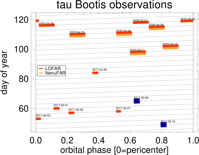
Figure 1: Orbital phase coverage for the observations of $\tau$ Boo b. The orbital phase was calculated using the ephemeris from Wang & Ford (2011) and is relative to periastron of $\tau$ Boo b. The LOFAR and NenuFAR observations are labeled in red and orange, respectively. The original LOFAR observations were taken between February 18, 2017 and March 25, 2017. The $\tau$ Boo LOFAR observations with the tentative detections are displayed as large dark-blue rectangles. The tentative detection of burst emission was seen on February 18, 2017 and the slow emission was seen on March 6, 2017. An arbitrary number of days was placed between the 2020 and 2017 observations for clarity.

3 Data Reduction

The raw beamformed exoplanet observations from NenuFAR are produced by coherently summing all the signals from each dipole antenna. They represent 125 GB / hour stored at the Nançay data center. The reduction pipeline applied to our data consisted in computing the 4 Stokes parameters (I, Q, U, and V), and applying RFI mitigation and correction of the time variations of the instrumental gain, before integrating the measurements on 250 ms $\times$ 48 kHz bins (i.e. 24 $\times$ 16 raw bins). The purpose of the RFI mitigation is to prevent polluted 3.05 $\times$ 10 ms bins to be included in the integrated 250 ms $\times$ 48 kHz bins, thus it is restricted to scales smaller than 250 ms in time and 48 kHz in frequency. RFI at larger scales are not eliminated at the reduction stage, and must be flagged in the post-processing stage. For the 2020 data, only the intensity (I), circular polarization (V) and linear polarization ($L=(Q^{2}+U^{2})^{1/2}$ were stored. The reduced data, flag masks, time and frequency ranges, and housekeeping data are stored as standard fits files, of volume $\sim$400 times smaller than the raw data, thus easy to post-process. This data is labeled as level 2 data (L2) whereas the level 1 data (L1) is the raw data. The raw data are then erased.

An example dynamic spectra of the L2 data for $\tau$ Boo can be found in Figure 2A. In this figure, lots of systematics are still clearly visible in the data. The source of many of the features is not yet well understood but several have a known origin. For example, the analog beams of NenuFAR are re-pointed every 6 minutes to ensure accurate source tracking. These re-pointings are clearly visible in the data as the baseline changes after every new pointing. The blobs above 30 MHz are caused by bright-sources in the grating lobes of NenuFAR.

(A)

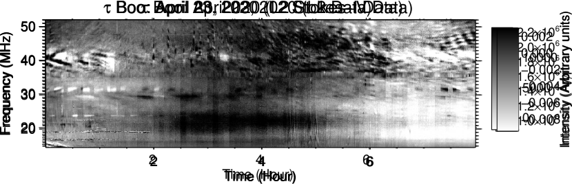
(B)

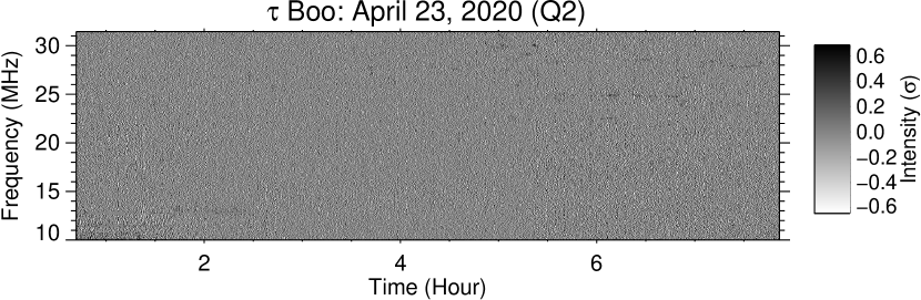
Figure 2: The dynamic spectra in Stokes V for the April 23, 2020 $\tau$ Boo observation with NenuFAR. (A.) Example of a pre-processed (L2) dynamic spectra. The intensity in the dynamic spectrum is in arbitrary units. (B.) Example of a high-pass filtered dynamic spectra. The dynamic spectrum is normalized by the standard deviation of the observations.

Next, the L2 data were processed using the BOREALIS (BeamfOrmed Radio Emission AnaLysIS) pipeline (Turner et al. 2017, 2019; Turner et al. 2021). We performed RFI mitigation using a similar setup as in T21. Due to the complexity of the NenuFAR data (e.g. six-minute pointing jumps), we did not correct for the time-frequency background of the observations. This will be done in future work. This limitation is the reason why we only search for bursty emission in this study. After RFI mitigation we re-binned the data to a time and frequency resolution of 1 second and 45 kHz, respectively. This rebinned data was then fed into the post-processing part of BOREALIS.

In order to determine the reliability of the NenuFAR data, we processed the pulsar (B0809+74) through the BOREALIS pipeline. In order to detect B0809+74 we perform an FFT on the RFI masked, de-dispersed (the data is de-disperse using the pulsar’s known dispersion measure), and rebinned data (we only rebinned the data in frequency). The FFT was computed using data from 40-50 MHz. Figure 3 shows an FFT of B0809+74 using NenuFAR data taken on April 23, 2020. The pulsar is detected with a signal-to-noise of $\sim$6 at its known period. Based on this result, we are confident that the pipeline masks the RFI adequately and will allow for the search for bursty signals from the exoplanet.

Figure 3: FFT of the pulsar B0809+74 for the NenuFAR data taken on taken on April 23, 2020. The known period is denoted as the dashed line and the pulsar is detected with a signal-to-noise of $\sim$6 around this period.

In the post-processing, we only searched for burst emission. A very detailed description of the burst emission observables can be found in Turner et al. (2019) and T21 and we describe them briefly below. The post-processing is performed on the absolute value of the corrected Stokes V data as defined in Turner et al. (2019). For burst emission, we only use the Q2 and Q4a-f observable quantities. The Q2 observable consists of one time series per beam (ON, OFF1, OFF2, and OFF3). It is obtained by high-pass filtering the dynamic spectrum. An example of a high-pass filtered dynamic spectrum for $\tau$ Boo can be found in Figure 2B. To search for faint emission, the high-pass filtered dynamic spectrum is integrated over a large frequency range (e.g., bin sizes of 10 MHz) to produce a time series. Q2 can be represented by a “scatter plot” comparing a pair of beams (e.g., the ON and one of the OFF beams) and is designed to find bursty emission (with time scales $<\sim$ 1 minute). The quantities Q4a to Q4f provide statistical measures of the bursts identified by the Q2 quantity. When examining Q4a-f, the ON and OFF time series are compared to each other; for this, we introduce the difference curve Q4f${}_{\text{Diff}}$=Q4f(ON)-Q4f(OFF). We then plot this curve against a reference curve computed from 10000 draws of purely Gaussian noise.

The post-processing was performed separately over 4 different frequency ranges (15 - 21 MHz, 15-52 MHz, 15-33 MHz, and 33-52 MHz). All other post-processing parameters are similar to those of T21. In this paper, we search for burst emission in the data that has binned to 1 second and highpass filtered with a smoothing timescale of 10 seconds. Therefore, only emission less than 10 seconds can be searched for in the data. T21 only observed burst emission at this same timescale.

4 Results

We searched for excess signal in the ON-beam both by eye and using the automated search procedure outlined in T21. We applied the same criteria as in Turner et al. 2019; Turner et al. 2021 for a possible detection. We do not find any burst emission in the NenuFAR observations for any of the probed wavelength ranges. The burst statistics were similar between all ON and OFF beams. An example of the diagnostics for a non-detection can be found in Figure 4, based on the April 23, 2020 NenuFAR observation, analyzed between 15-32 MHz. The ON-OFF and OFF-OFF difference curves are very similar to each other and all curves are systematically non-Gaussian. We performed a red-noise analysis on the Q2 time series for the ON and OFF beams using the wavelet technique of Carter & Winn (2009) as implemented in the EXOMOP code by Turner et al. (2016b). The wavelet technique assumes that the time series is an additive combination of noise with Gaussian white noise and red noise (characterized as a power spectral density proportional to $1/f^{\alpha}$). We find that the red and white noise components are nearly equal in magnitude. We will investigate this systematic noise in the data in future work.

(a)

(b)

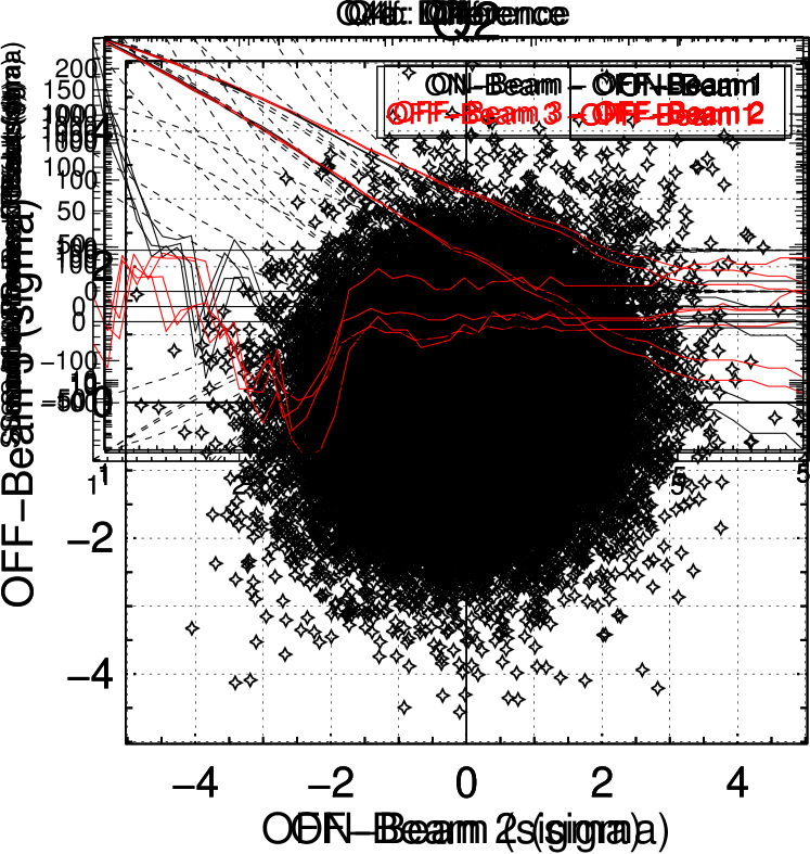
(c)

(d)

(e)

(f)

Figure 4: Non-detection of burst emission for $\tau$ Boo in the April 15, 2020 NenuFAR observation between 15-32 MHz in Stokes V. Panel a: Q2 for the ON-beam vs the OFF-beam 2. Panel b: Q2 for the OFF-beam 1 vs the OFF-beam 2. Panel c: Q4a (number of peaks). Panel d: Q4b (power of peaks). Panel e: Q4e (peak offset). Panel f: Q4f (peak offset). For panels c to f the black lines are the ON-beam difference with the OFF beam 2 and the red lines are the OFF-beam difference. The dashed lines are statistical limits (1, 2, 3$\sigma$) of the difference between all the Q4 values derived using two different Gaussian distributions (each performed 10000 times). We do not see any excess signal in the ON-beam compared to the OFF-beams.

5 Discussion

We do not detect any burst emission in our NenuFAR observations. This is consistent with the simultaneous LOFAR observations that also did not detect any bursty emission that will be presented elsewhere. The original LOFAR observations (T21) only detected burst emission flux during one four-hour observation centered around an orbital phase of 0.8 (Figure 1). All the NenuFAR observations besides April 15, 2020 are consistent with this finding. Based on T21, one might have expected to detect bursty emission at orbital phase 0.8, i.e. for the NenuFAR observation of April 15, 2020.

There are many different degenerate reasons for our non-detection of burst emission from $\tau~{}$Boo:

1. It is possible that the original 3.2$\sigma$ bursty signal detected by T21 was caused by an unknown instrumental systematic or statistical anomaly. An extensive systematic study was undertaken by T21 and no plausible cause for a false positive signal could be identified for the bursty emission signature. In the future, a statistical comparison between many LOFAR and NenuFAR datasets may shed light on this issue.

2. An extended, evaporating atmosphere can lead to conditions in the planetary magnetosphere that doesn’t allow the CMI mechanism to operate (the local electron plasma frequency is greater than the local electron cyclotron frequency, $\omega_{p}$ $>$ $\omega_{c}$; Grießmeier et al. 2023, e.g.). However, for a planet as massive as $\tau~{}$Boo b, this effect is not expected (Weber et al., 2018). On the other hand, if the planetary magnetic field is as low as estimated by Reiners & Christensen (2010), the condition for the CMI to operate is only marginally fulfilled (Weber et al., 2018, Figure 5), and temporal variations could, in principle, lead to a situation where the emission does not operate continuously. It is worth noting that Kao et al. (2016, 2018) showed that the Reiners & Christensen (2010) magnetic field predictions may not be applicable for all brown dwarfs. However, it is currently unclear if the contradiction found by Kao et al. (2016, 2018) extends to hot Jupiters such as $\tau$ Boo b. More work is needed to understand this limitation.

3. The observations could have been taken at an unfavorable rotational phase of the star. Planetary radio emission is triggered by the interaction of the planetary magnetosphere with the magnetized stellar wind (Zarka et al. 2001; Zarka 2018). For this reason, the expected intensity of the planetary radio emission differs greatly with stellar rotation (e.g. Grießmeier et al. 2005b; Grießmeier et al. 2007a; Fares et al. 2010; Vidotto et al. 2012; See et al. 2015; Strugarek et al. 2022). See et al. (2015) showed that the expected radio flux of $\tau~{}$Boo b can disappear entirely for certain stellar rotation phases. We cannot rule out variability in the radio signal due to observing at different stellar rotation phases (no stellar differential rotation constraints exist during our 2020 observing campaign).

4. The observations could have been taken at an unfavorable time in the stellar magnetic cycle. The host star $\tau~{}$Boo is known to undergo a rapid magnetic cycle of 120 days (Jeffers et al. 2018). Similarly to the stellar rotation, this is expected to modulate the planetary radio emission (e.g. Fares et al. 2009; Vidotto et al. 2012; See et al. 2015; Elekes & Saur 2023). See et al. (2015) also found that the expected radio flux of $\tau~{}$Boo b (at optimal stellar longitude) can vary by a factor of $\sim$5 along the stellar magnetic cycle. Most recently, Elekes & Saur (2023) showed that a magnetic polarity reversal of the host star towards an anti-aligned field configuration would result in the planetary radio emission being below the detection threshold of NenuFAR. However, no stellar magnetic field data of $\tau$ Boo exists during our 2020 observing campaign. Therefore, we cannot rule out variability in the radio signal due to observing at different moments of the stellar magnetic cycle.

5. Unlike Jupiter’s decametric emission (Zarka 1998), the planetary emission from $\tau$ Boo might not always be on. This would imply that the magnetosphere dynamics of $\tau$ Boo b would be different than that of Jupiter. For example, the density of the magnetosphere could be variable and perhaps temporarily become void of particles.

A large follow-up campaign is needed to disentangle the true cause of the possible variability of the planetary radio emission. Multi-site observations are highly encouraged to rule out instrumental systematics. Monitoring the planet throughout its orbit and the stellar magnetic cycle is necessary to disentangle the competing effects. There is also a need for measurements of the stellar magnetic field taken throughout the radio follow-up campaign. Such a coordinated campaign is currently ongoing, using NenuFAR for the radio emission, and the TBL/Neo-Narval to monitor the magnetic field of the host star.

With our non-detection, we can place an upper limit on the radio emission from the $\tau$ Boo system at the time of the observations. Since NenuFAR is still in early commissioning the system equivalent flux density (SEFD) is currently not well characterized. Therefore, we will approximate our upper limit of NenuFAR based-off the sensitivity limit found for LOFAR in Turner et al. (2019). The theoretical sensitivity limit of LOFAR for broadband bursts

$$\sigma_{LOFAR}= \frac{S_{Sys}}{N\sqrt{b\tau}},$$ (1)

$$\sigma_{LOFAR}= \frac{40kJy}{24\sqrt{1\ sec\times 18\ MHz}}=393\ mJy$$ (2)

where $N$ is the number of stations (24), $b$ is the bandwidth (18 MHz using the 15-33 MHz frequency range), $\tau$ is the timing resolution (1 sec), and $S_{Sys}$ is the station SEFD with a value of 40 kJy (van Haarlem et al. 2013). Turner et al. (2019) measured the sensitivity limit of LOFAR to be $1.3\times\sigma_{LOFAR}$ and we will use this value below. For the burst emission from NenuFAR, we find a 3$\sigma$ flux upper limit of 1.5 Jy and 590 mJy assuming NenuFAR is as sensitive and twice as sensitive as LOFAR, respectively. This limit is a conservative preliminary estimate as NenuFAR is expected to be more sensitive (at least 2–5$\times$) than LOFAR between 15–30 MHz. In the future, the SEFD of NenuFAR will be accurately measured and we will perform a comprehensive sensitivity estimation using Jupiter radio emission simulated as if it was an exoplanet (using the same method used to obtain the sensitivity limit for LOFAR observations in Turner et al. 2019). Therefore, we expect to have a more precise upper limit in future work.

The current NenuFAR observations are informative on the nature of $\tau$ Boo b’s radio emission. The original tentative detection of burst emission from T21 was observed to have a flux density of 890 mJy. Therefore, we would have detected the burst emission of $\tau$ Boo b (in the absence of variability, see above) at $\sim$4.5 $\sigma$ using the NenuFAR conservative sensitivity limit (2$\times$ as sensitive as LOFAR) of $\sim$200 mJy. We also expected to observe bursty emission at an orbital phase (e.g. 0.8) similar to that found in T21 and validated in the model by Ashtari et al. (2022). Therefore, the observed phases and the current upper limits can be used as priors in theoretical predictions (e.g Elekes & Saur 2023; Ashtari et al. 2022) in the expected variability of $\tau$ Boo b’s radio emission.

6 Conclusions and Perspectives

In this study, we search for bursty emission from the $\tau$ Boo exoplanetary system using NenuFAR during its commissioning phase in 2020. This is the first exoplanet observation from NenuFAR to be published. These observations are part of a large ongoing follow-up campaign to confirm the tentative detections of radio emission from $\tau$ Boo observed by LOFAR (Turner et al. 2021). We do not detect any bursty emission in the NenuFAR observations and the reason for this non-detection is degenerate. Possible interpretations include the possibility that the original burst detection was an unknown systematic error or that radio emission from $\tau$ Boo b is variable in time. Further analysis on the NenuFAR data and more observations are needed to fully understand the radio emission from the $\tau$ Boo system. Such observations are currently ongoing.

References

- Alexander et al. (2016) Alexander R. D., Wynn G. A., Mohammed H., Nichols J. D., Ercolano B., 2016, Magnetospheres of hot Jupiters: hydrodynamic models and ultraviolet absorption, MNRAS, 456, 2766
- Ashtari et al. (2022) Ashtari R., Sciola A., Turner J. D., Stevenson K., 2022, Detecting Magnetospheric Radio Emission from Giant Exoplanets, ApJ, 939, 24
- Bastian et al. (2000) Bastian T. S., Dulk G. A., Leblanc Y., 2000, A Search for Radio Emission from Extrasolar Planets, ApJ, 545, 1058
- Bastian et al. (2018) Bastian T. S., Villadsen J., Maps A., Hallinan G., Beasley A. J., 2018, Radio Emission from the Exoplanetary System Eridani, ApJ, 857, 133
- Blanco-Pozo et al. (2023) Blanco-Pozo J., et al., 2023, The CARMENES search for exoplanets around M dwarfs. A long-period planet around GJ 1151 measured with CARMENES and HARPS-N data, AA, 671, A50
- Bondonneau et al. (2021) Bondonneau L., et al., 2021, Pulsars with NenuFAR: Backend and pipelines, AA, 652, A34
- Callingham et al. (2021) Callingham J. R., et al., 2021, The population of M dwarfs observed at low radio frequencies, Nature Astronomy, 5, 1233
- Carter & Winn (2009) Carter J. A., Winn J. N., 2009, Parameter Estimation from Time-series Data with Correlated Errors: A Wavelet-based Method and its Application to Transit Light Curves, ApJ, 704, 51
- Cauley et al. (2019) Cauley P. W., Shkolnik E. L., Llama J., Lanza A. F., 2019, Magnetic field strengths of hot Jupiters from signals of star-planet interactions, Nature Astronomy, p. 408
- Cendes et al. (2022) Cendes Y., Williams P. K. G., Berger E., 2022, A Pilot Radio Search for Magnetic Activity in Directly Imaged Exoplanets, AJ, 163, 15
- Elekes & Saur (2023) Elekes F., Saur J., 2023, Space environment and magnetospheric Poynting fluxes of the exoplanet Boötis b, arXiv e-prints, p. arXiv:2301.05015
- Fares et al. (2009) Fares R., et al., 2009, Magnetic cycles of the planet-hosting star Bootis - II. A second magnetic polarity reversal, MNRAS, 398, 1383
- Fares et al. (2010) Fares R., et al., 2010, Searching for star-planet interactions within the magnetosphere of HD189733, MNRAS, 406, 409
- Farrell et al. (1999) Farrell W. M., Desch M. D., Zarka P., 1999, On the possibility of coherent cyclotron emission from extrasolar planets, J. Geophys. Res., 104, 14025
- Grießmeier (2015) Grießmeier J.-M., 2015, Detection Methods and Relevance of Exoplanetary Magnetic Fields, in Astrophysics and Space Science Library, eds Lammer H., Khodachenko M., , Astrophysics and Space Science Library Vol. 411, p. 213, doi:10.1007/978-3-319-09749-7˙11
- Grießmeier (2017) Grießmeier J.-M., 2017, The search for radio emission from giant exoplanets, in Planetary Radio Emissions VIII, eds G. Fischer and G. Mann and M. Panchenko and P. Zarka, Austrian Academy of Sciences Press, Vienna, pp 285–300
- Grießmeier (2018) Grießmeier J. M., 2018, Future Exoplanet Research: Radio Detection and Characterization, in Handbook of Exoplanets, ISBN 978-3-319-55332-0. Springer International Publishing AG, part of Springer Nature, 2018, id.159, p. 159, doi:10.1007/978-3-319-55333-7˙159
- Grießmeier et al. (2005a) Grießmeier J.-M., Stadelmann A., Motschmann U., Belisheva N. K., Lammer H., Biernat H. K., 2005a, Cosmic Ray Impact on Extrasolar Earth-Like Planets in Close-in Habitable Zones, Astrobiology, 5, 587
- Grießmeier et al. (2005b) Grießmeier J.-M., Motschmann U., Mann G., Rucker H. O., 2005b, The influence of stellar wind conditions on the detectability of planetary radio emissions, AA, 437, 717
- Grießmeier et al. (2007a) Grießmeier J. M., Preusse S., Khodachenko M., Motschmann U., Mann G., Rucker H. O., 2007a, Exoplanetary radio emission under different stellar wind conditions, Planetary and Space Science, 55, 618
- Grießmeier et al. (2007b) Grießmeier J.-M., Zarka P., Spreeuw H., 2007b, Predicting low-frequency radio fluxes of known extrasolar planets, AA, 475, 359
- Grießmeier et al. (2023) Grießmeier J.-M., Erkaev N. V., Weber C., Lammer H., Ivano V. A., Odert P., 2023, Required conditions for an exoplanet to emit radio waves and implications for observational campaigns, in Planetary Radio Emissions IX, ed. C. K. Louis, C. M. Jackman, G. Fischer, A. H. Sulaiman, P. Zucca, Austrian Academy of Sciences Press, Vienna, doi:https://doi.org/10.25546/103090
- Hallinan et al. (2013) Hallinan G., Sirothia S. K., Antonova A., Ishwara-Chandra C. H., Bourke S., Doyle J. G., Hartman J., Golden A., 2013, Looking for a Pulse: A Search for Rotationally Modulated Radio Emission from the Hot Jupiter, Boötis b, ApJ, 762, 34
- Heald et al. (2015) Heald G. H., et al., 2015, The LOFAR Multifrequency Snapshot Sky Survey (MSSS). I. Survey description and first results, AA, 582, A123
- Hess & Zarka (2011) Hess S. L. G., Zarka P., 2011, Modeling the radio signature of the orbital parameters, rotation, and magnetic field of exoplanets, AA, 531, A29
- Hindle et al. (2021) Hindle A. W., Bushby P. J., Rogers T. M., 2021, The Magnetic Mechanism for Hotspot Reversals in Hot Jupiter Atmospheres, ApJ, 922, 176
- Jeffers et al. (2018) Jeffers S. V., et al., 2018, The relation between stellar magnetic field geometry and chromospheric activity cycles - II The rapid 120-day magnetic cycle of Bootis, MNRAS, 479, 5266
- Kao et al. (2016) Kao M. M., Hallinan G., Pineda J. S., Escala I., Burgasser A., Bourke S., Stevenson D., 2016, Auroral Radio Emission from Late L and T Dwarfs: A New Constraint on Dynamo Theory in the Substellar Regime, ApJ, 818, 24
- Kao et al. (2018) Kao M. M., Hallinan G., Pineda J. S., Stevenson D., Burgasser A., 2018, The Strongest Magnetic Fields on the Coolest Brown Dwarfs, The Astrophysical Journal Supplement Series, 237, 25
- Knierim et al. (2022) Knierim H., Batygin K., Bitsch B., 2022, Shallowness of circulation in hot Jupiters. Advancing the Ohmic dissipation model, AA, 658, L7
- Lammer et al. (2009) Lammer H., et al., 2009, What makes a planet habitable?, A&Ar, 17, 181
- Lazio et al. (2004) Lazio W. T. J., Farrell W. M., Dietrick J., Greenlees E., Hogan E., Jones C., Hennig L. A., 2004, The Radiometric Bode’s Law and Extrasolar Planets, ApJ, 612, 511
- Lazio et al. (2016) Lazio T. J. W., Shkolnik E., Hallinan G., Planetary Habitability Study Team 2016, Technical report, Planetary Magnetic Fields: Planetary Interiors and Habitability
- Lazio et al. (2019) Lazio J., et al., 2019, Magnetic Fields of Extrasolar Planets: Planetary Interiors and Habitability, BAAS, 51, 135
- Lecavelier des Etangs et al. (2013) Lecavelier des Etangs A., Sirothia S. K., Gopal-Krishna Zarka P., 2013, Hint of 150 MHz radio emission from the Neptune-mass extrasolar transiting planet HAT-P-11b, A&A, 552, A65
- Lynch et al. (2018) Lynch C. R., Murphy T., Lenc E., Kaplan D. L., 2018, The detectability of radio emission from exoplanets, MNRAS, 478, 1763
- Manchester et al. (2005) Manchester R. N., Hobbs G. B., Teoh A., Hobbs M., 2005, The Australia Telescope National Facility Pulsar Catalogue, AJ, 129, 1993
- Mauduit et al. (2023) Mauduit E., Zarka P., Grießmeier J.-M., Turner J. D., 2023, PALANTIR: an updated prediction tool for exoplanetary radioemissions, in Planetary Radio Emissions IX, ed. C. K. Louis, C. M. Jackman, G. Fischer, A. H. Sulaiman, P. Zucca, Austrian Academy of Sciences Press, Vienna, doi:https://doi.org/10.25546/103092
- McIntyre et al. (2019) McIntyre S. R. N., Lineweaver C. H., Ireland M. J., 2019, Planetary magnetism as a parameter in exoplanet habitability, MNRAS, 485, 3999
- Meadows & Barnes (2018) Meadows V. S., Barnes R. K., 2018, in eds Deeg H. J., Belmonte J. A., , , Handbook of Exoplanets. p. 57, doi:10.1007/978-3-319-55333-7_57
- Narang et al. (2023) Narang M., Oza A. V., Hakim K., Manoj P., Banyal R. K., Thorngren D. P., 2023, Radio-loud Exoplanet-exomoon Survey: GMRT Search for Electron Cyclotron Maser Emission, AJ, 165, 1
- Nichols (2012) Nichols J. D., 2012, Candidates for detecting exoplanetary radio emissions generated by magnetosphere-ionosphere coupling, MNRAS, 427, L75
- Pérez-Torres et al. (2021) Pérez-Torres M., et al., 2021, Monitoring the radio emission of Proxima Centauri, AA, 645, A77
- Perna et al. (2010) Perna R., Menou K., Rauscher E., 2010, Magnetic Drag on Hot Jupiter Atmospheric Winds, ApJ, 719, 1421
- Pineda & Villadsen (2023) Pineda J. S., Villadsen J., 2023, Coherent radio bursts from known M-dwarf planet-host YZ Ceti, Nature Astronomy,
- Rauscher & Menou (2013) Rauscher E., Menou K., 2013, Three-dimensional Atmospheric Circulation Models of HD 189733b and HD 209458b with Consistent Magnetic Drag and Ohmic Dissipation, APJ, 764, 103
- Reiners & Christensen (2010) Reiners A., Christensen U. R., 2010, A magnetic field evolution scenario for brown dwarfs and giant planets, AA, 522, A13
- Route (2019) Route M., 2019, The Rise of ROME. I. A Multiwavelength Analysis of the Star-Planet Interaction in the HD 189733 System, ApJ, 872, 79
- Schneider et al. (2011) Schneider J., Dedieu C., Le Sidaner P., Savalle R., Zolotukhin I., 2011, Defining and cataloging exoplanets: the exoplanet.eu database, A&A, 532, A79
- See et al. (2015) See V., Jardine M., Fares R., Donati J.-F., Moutou C., 2015, Time-scales of close-in exoplanet radio emission variability, MNRAS, 450, 4323
- Sirothia et al. (2014) Sirothia S. K., Lecavelier des Etangs A., Gopal-Krishna Kantharia N. G., Ishwar-Chandra C. H., 2014, Search for 150 MHz radio emission from extrasolar planets in the TIFR GMRT Sky Survey, A&A, 562, A108
- Strugarek et al. (2022) Strugarek A., et al., 2022, MOVES - V. Modelling star-planet magnetic interactions of HD 189733, MNRAS, 512, 4556
- Treumann (2006) Treumann R. A., 2006, The electron-cyclotron maser for astrophysical application, AAr, 13, 229
- Trigilio et al. (2023) Trigilio C., et al., 2023, Star-Planet Interaction at radio wavelengths in YZ Ceti: Inferring planetary magnetic field, arXiv e-prints, p. arXiv:2305.00809
- Turner et al. (2016a) Turner J. D., Christie D., Arras P., Johnson R. E., Schmidt C., 2016a, Investigation of the environment around close-in transiting exoplanets using CLOUDY, MNRAS, 458, 3880
- Turner et al. (2016b) Turner J. D., et al., 2016b, Ground-based near-UV observations of 15 transiting exoplanets: constraints on their atmospheres and no evidence for asymmetrical transits, MNRAS, 459, 789
- Turner et al. (2017) Turner J. D., Grießmeier J.-M., Zarka P., Vasylieva I., 2017, The search for radio emission from exoplanets using LOFAR low-frequency beam-formed observations: Data pipeline and preliminary results for the 55 Cnc system, in Planetary Radio Emissions VIII, eds G. Fischer and G. Mann and M. Panchenko and P. Zarka, Austrian Academy of Sciences Press, Vienna, pp 301–313
- Turner et al. (2019) Turner J. D., Grießmeier J.-M., Zarka P., Vasylieva I., 2019, The search for radio emission from exoplanets using LOFAR beam-formed observations: Jupiter as an exoplanet, AA, 624, A40
- Turner et al. (2021) Turner J. D., et al., 2021, The search for radio emission from the exoplanetary systems 55 Cancri, Andromedae, and Boötis using LOFAR beam-formed observations, AA, 645, A59
- Vasylieva (2015) Vasylieva I., 2015, Pulsars and transients survey, and exoplanet search at low-frequencies with the UTR-2 radio telescope: methods and first results, Theses, Paris Observatory, https://tel.archives-ouvertes.fr/tel-01246634
- Vedantham et al. (2020) Vedantham H. K., et al., 2020, Coherent radio emission from a quiescent red dwarf indicative of star-planet interaction, Nature Astronomy,
- Vidotto et al. (2012) Vidotto A. A., Fares R., Jardine M., Donati J. F., Opher M., Moutou C., Catala C., Gombosi T. I., 2012, The stellar wind cycles and planetary radio emission of the Boo system, MNRAS, 423, 3285
- Wang & Ford (2011) Wang J., Ford E. B., 2011, On the eccentricity distribution of short-period single-planet systems, MNRAS, 418, 1822
- Weber et al. (2017) Weber C., et al., 2017, On the Cyclotron Maser Instability in Magnetospheres of Hot Jupiters - Influence of ionosphere models, in Planetary Radio Emissions VIII, eds G. Fischer and G. Mann and M. Panchenko and P. Zarka, Austrian Academy of Sciences Press, Vienna, pp 317–329, doi:10.1553/PRE8s317
- Weber et al. (2018) Weber C., Erkaev N. V., Ivanov V. A., Odert P., Grießmeier J.-M., Fossati L., Lammer H., Rucker H. O., 2018, Supermassive hot Jupiters provide more favourable conditions for the generation of radio emission via the cyclotron maser instability - a case study based on Tau Bootis b, MNRAS, 480, 3680
- Winglee et al. (1986) Winglee R. M., Dulk G. A., Bastian T. S., 1986, A search for cyclotron maser radiation from substellar and planet-like companions of nearby stars, ApJl, 309, L59
- Wu & Lee (1979) Wu C. S., Lee L. C., 1979, A theory of the terrestrial kilometric radiation, ApJ, 230, 621
- Yantis et al. (1977) Yantis W. F., Sullivan III W. T., Erickson W. C., 1977, A Search for Extra-Solar Jovian Planets by Radio Techniques, in Bulletin of the American Astronomical Society, p. 453
- Zarka (1998) Zarka P., 1998, Auroral radio emissions at the outer planets: Observations and theories, JGR, 103, 20159
- Zarka (2007) Zarka P., 2007, Plasma interactions of exoplanets with their parent star and associated radio emissions, Planetary and Space Science, 55, 598
- Zarka (2018) Zarka P., 2018, Star-Planet Interactions in the Radio Domain: Prospect for Their Detection, in Handbook of Exoplanets, p. 22, doi:10.1007/978-3-319-55333-7˙22
- Zarka et al. (1997) Zarka P., et al., 1997, Ground-Based High Sensitivity Radio Astronomy at Decameter Wavelengths, in Planetary Radio Emission IV, eds Rucker, H. O. and Bauer, S. J. and Lecacheux, A., p. 101
- Zarka et al. (2001) Zarka P., Treumann R. A., Ryabov B. P., Ryabov V. B., 2001, Magnetically-Driven Planetary Radio Emissions and Application to Extrasolar Planets, Astrophys. Space. Sci., 277, 293
- Zarka et al. (2004) Zarka P., Cecconi B., Kurth W. S., 2004, Jupiter’s low-frequency radio spectrum from Cassini/Radio and Plasma Wave Science (RPWS) absolute flux density measurements, Journal of Geophysical Research (Space Physics), 109, A09S15
- Zarka et al. (2015) Zarka P., Lazio J., Hallinan G., 2015, Magnetospheric Radio Emissions from Exoplanets with the SKA, Advancing Astrophysics with the Square Kilometre Array (AASKA14), p. 120
- Zarka et al. (2020) Zarka P., et al., 2020, The low-frequency radio telescope NenuFAR, in URSI General Assembly, p. session J01: New Telescopes on the Frontier
- van Haarlem et al. (2013) van Haarlem M. P., et al., 2013, LOFAR: The LOw-Frequency ARray, AA, 556, A2