GReAT: A Graph Regularized Adversarial Training Method

Abstract

This paper proposes a regularization method called GReAT, Graph Regularized Adversarial Training, to improve deep learning models’ classification performance. Adversarial examples are a well-known challenge in machine learning, where small, purposeful perturbations to input data can mislead models. Adversarial training, a powerful and one of the most effective defense strategies, involves training models with both regular and adversarial examples. However, it often neglects the underlying structure of the data. In response, we propose GReAT, a method that leverages data graph structure to enhance model robustness. GReAT deploys the graph structure of the data into the adversarial training process, resulting in more robust models that better generalize its testing performance and defend against adversarial attacks. Through extensive evaluation on benchmark datasets, we demonstrate GReAT’s effectiveness compared to state-of-the-art classification methods, highlighting its potential in improving deep learning models’ classification performance.

organization=Electrical and Computer Engineering Delaware, University of Delaware,
addressline=139 The Green, city=Newark, postcode=19716, state=DE, country=United States

1 Introduction

Deep learning is a subset of machine learning (ML) that uses artificial neural networks with multiple layers and neurons to analyze and learn from large amounts of data. Deep learning algorithms automatically learn and extract relevant features from the data to make predictions. The feature extraction process allows algorithms to achieve higher levels of accuracy and perform more complex tasks. In the last decades, deep learning has achieved impressive results in various domains, including image and text classification, speech recognition, image generation, and natural language processing ^{1, 2, 3}. Supervised learning methods achieved the most successful results. In this learning technique, the model is trained on a labeled dataset, meaning the input data is accompanied by its corresponding output labels. Supervised learning aims to predict new, unseen data based on the patterns learned from the labeled data. Deep neural networks adjust the weights and biases of the network through back-propagation using output labels and original labels.

Semi-supervised learning combines both supervised and unsupervised learning techniques. In this type of learning, a model is trained on a data set that has labeled and unlabeled instances. The goal is to use the labeled data to make predictions on unlabeled and new, unseen, data. This method is used often when there is a limited amount of labeled data but a larger amount of unlabeled data. There are various algorithms for propagating the labels through the graph, such as label propagation ^{4, 5}, pseudo-labeling ⁶, transductive SVMs ⁷, and self-training ⁸. Label propagation provides outstanding performance for semi-supervised learning to classify graph nodes. It is based on the idea that a node’s labels can be propagated to its neighbors based on the assumption that nodes with similar labels are more likely to be connected.

Despite their significant success, deep learning models are known to be vulnerable to adversarial examples. These examples are created by adding small, carefully chosen perturbations to the input data. The perturbed data remains visually similar to the original data but is misclassified by the model ^{9, 10, 11}. The existence of adversarial examples has drawn significant attention to the machine-learning community. Showing the vulnerabilities of machine learning algorithms has opened critical research areas in the attack and robustness areas. Studies have shown that adversarial attacks are highly effective on many existing AI systems, especially on image classification tasks; ^{12, 13, 10, 14, 15, 16, 17, 18}. For instance, ¹² show that even small perturbations in input testing images can significantly change the classification accuracy.

⁹ attempts to explain the existence of adversarial examples and proposes one of the first efficient attack algorithms in white–box settings. ¹⁹ proposed projected gradient descent (PGD) as a universal first-order adversarial attack. They stated that network architecture and capacity play a significant role in adversarial robustness. Notable other popular adversarial attack methods are the Carlini-Wagner Attack (CW) ²⁰, Basic Iterative Method (BIM) ²¹, and Momentum Iterative Attack ²². ²³ show the transferability of black-box attacks among different ML models.

Adversarial defense mechanisms can broadly be classified into two categories. The first category predominantly centers on pre-processing techniques tailored for DL models, to mitigate adversarial perturbations in the adversarial examples. Methods in this category include feature denoising, ²⁴, Fourier filtering, ²⁵, and random resizing coupled with random padding, ²⁶, among others. The second category targets modifications in the architecture of neural networks, including alterations in activation functions, ²⁷, adaptations in learning processes like distillation, ²⁸, the introduction of novel loss functions, ²⁹, and adjustments in training procedures, ⁹.

The existing literature underscores the effectiveness of unlabeled samples to enhance deep learning performance, ^{30, 31, 32, 4}. Additionally, studies show that unlabeled data improve adversarial robustness, ³³. Motivated by these insights, we propose a Graph-Regularized Adversarial Training method (GReAT) to improve the robustness performance. The proposed method utilizes the structural information from the input data to improve the robustness of deep learning models against adversarial attacks. The main idea within GReAT is to construct a graph representation of clean data with an adversarial neighborhood, where each node represents a data point, and the edges encode the similarity between the nodes. This approach allows us to incorporate the structural information from the data into the training process, which helps create robust classification models. To evaluate the effectiveness of our approach, we conduct experiments on data sets: TensorFlow’s flower data set ³⁴ and CIFAR-10 ³⁵. We compare GReAT with several state-of-the-art methods. The results show that the proposed approach consistently outperforms the baselines regarding accuracy and robustness against adversarial attacks. Our proposed GReAT graph-based semi-supervised learning approach for adversarial training provides a promising direction for improving the robustness of deep learning models against adversarial attacks.

2 Background and Related Works

This section covers the relevant background and related works. In particular, we cover deep learning and semi-supervised learning, adversarial learning, and graph-based semi-supervised learning.

2.1 Deep Learning and Semi-supervised Learning

DL models are complex non-linear mapping functions between input and output. They consist of multiple layers and neurons with activation functions. They extract features from input samples and predict labels based on those features. Neural networks are trained using vast amounts of labeled data and can learn and improve their performance over time utilizing backpropagation algorithms.

The following equation represents the prediction process of the classical deep learning paradigm:

$$\bm{Y}:f(\bm{X},\bm{\theta},\bm{b}),$$ (1)

where $\bm{X}$ is the data fed into the neural network $f$, $\bm{\theta}$ represent the values assigned to the connections between the neurons in the network, and $\bm{b}$ is the offsets applied to the input data. The output is the result produced by the neural network after processing the input data through its layers of neurons.

Semi-supervised learning uses labeled and unlabeled data to train a model. The following representation shows the prediction process of semi-supervised learning:

$$\bm{Y}:f(\bm{X_{l}},\bm{X_{ul}},\bm{\theta},\bm{b}),$$ (2)

where $\bm{X_{l}}$ is the labeled data and $\bm{X_{ul}}$ is the unlabeled data. The weights and biases are the same as in supervised-learning learning. The output is the result produced by the model after processing the labeled and unlabeled data through its layers of neurons. A label assignment procedure typically exists in semi-supervised learning to annotate the unlabeled data. This procedure employs a smoothing function or similarity metrics to assign the label of the most similar labeled sample to the unlabeled sample, ⁵.

2.2 Adversarial Learning

A data instance $\bm{x}^{\prime}$ is considered an adversarial example of a natural instance $\bm{x}$ when $\bm{x}^{\prime}$ is close to $\bm{x}$, under a specific distance metric, while $f(\bm{x}^{\prime})\neq y$, where $y$ is the label of $\bm{x}$, ³⁶. Formally, an adversarial example of $\bm{x}$ is can be defined as

$$\bm{x}^{\prime}:D(\bm{x}^{\prime},\bm{x})<\epsilon,f(\bm{x}^{\prime})\neq y,$$ (3)

where $D(\cdot,\cdot)$ represents a distance metric, such as the $\lVert\cdot\rVert_{2}$ norm, and $\epsilon$ is a distance constraint, which limits the amount of allowed perturbations. Since the existence of adversarial examples is a significant threat to DL models, adversarial attack and defense algorithms are intensively investigated to improve the robustness and security of such models.

For instance, FGSM, by ⁹, was proposed to generate adversarial samples and attack DL models. The PGD algorithm, an iterative version of the FGSM attack, was proposed to generate adversarial samples by maximizing the loss increment within an $L_{\infty}$ norm-ball, ³⁷. Although many defense methods have been proposed, adversarial training is the most efficient approach against adversarial attacks, ^{9, 37}. ⁹ proposed using adversarial attack samples during training so that the classifier can learn the features of adversarial examples and their perturbations. The classifier’s robustness against adversarial attacks is substantially enhanced due to the integration of adversarial examples in the training phase. It effectively empowers the classifier to develop a more robust defense mechanism against adversarial instances. Formally, adversarial training is defined as

$$\bm{\theta^{*}}=\operatorname*{arg\,min}_{\theta\in\Theta}\frac{1}{L}\sum_{i=1}^{L}\max_{\textsf{D}(\bm{x}^{\prime}_{i},\bm{x}_{i})<\epsilon}\ell_{adv}(\theta,\bm{x}^{\prime}_{i},y_{i}).$$ (4)

The above equation states a min-max procedure under the specific distance constraint. In the inner maximization component, the adversarial training seeks an adversarial sample $\bm{x}^{\prime}_{j}$ to maximize the loss $\ell_{adv}$, under the distance metric $D(\bm{x}^{\prime}_{j},\bm{x}_{j})<\epsilon$, given the natural sample $\bm{x}_{j}$. The outer minimization seeks the optimal gradient $\theta^{*}$ that yields the global minimum empirical loss. In their work, Madry et al. iteratively applies the PGD algorithm during training to search for strong adversarial samples to maximize $\ell_{adv}$. This helps the model yield improved robustness against PGD and FGSM attacks. Adversarial training with PGD is considered one of the strongest defense methods, ³⁷.

2.3 Graph-based Semi-supervised Learning

Graph-based semi-supervised learning uses labeled and unlabeled data to train DL models, ^{30, 32, 38, 39, 40, 41}. This approach uses a small amount of labeled data and a large amount of unlabeled data to learn the graph structure of the given data. A given graph can be represented as $G=(V,E,W)$, where $V$ indicates data points as vertices, $E$ represents edges between data points, and $W$ is the edge weight matrix. The edges between the vertices are created on the basis of a similarity metric between the data points. Graph-based semi-supervised learning aims to use the graph structure and the labeled data to learn the label for the unlabeled data points. This technique is typically done by propagating the labels from the labeled data points to the unlabeled data points through the similarity graph of the entire data, ^{31, 42, 5, 41}.

In graph-based semi-supervised learning, label propagation is often used to classify nodes in a graph when only a few nodes have been labeled. This method starts with the labeled nodes and propagates their labels to their neighbors. The labels are then iteratively propagated repeatedly until the mapping function converges and the entire graph is labeled. As shown in ⁵, the loss function of the graph-based semi-supervised learning can be represented as:

$$\sum_{i=1}^{L}\ell(\theta,\bm{x}_{i},y_{i})+\lambda\sum_{i,j}w_{i,j}\lVert h(x_{i})-h(x_{j})\rVert^{2},$$ (5)

where the first term represents the standard supervised loss while the second term represents the penalty of the neighborhood loss. Note that $w_{ij}$ represents the similarity between different instances and $\lambda$ controls the contribution of neighborhood regularization. When $\lambda=0$, the loss term becomes the standard supervised loss. The penalty amount depends on the similarity between instance $\bm{x_{i}}$ and its neighbors. Also, $h$ represents a lookup table that contains all samples and similarity weights. It can be obtained with a closed-form solution, according to ⁴².

³⁸ proposed embedding samples instead of using lookup tables by extending the regularization term in the Eq. 5. The regularization term becomes $\lambda\sum_{i,j}\alpha_{i,j}\lVert g_{\theta}(x_{i})-g_{\theta}(x_{j})\rVert^{2}$, where $g_{\theta}(\cdot)$ indicates the embedding of samples generated by a neural network. Transforming the regularization term by transitioning from $f$ to $g$ leverages stronger constraints on the neural network, according to ⁵.

Here, we extend Eq. 5 by replacing the lookup table term with the embedding term in the regularization component and defining a general neighbor similarity metric. This approach yields

$$\sum_{i=1}^{L}\ell(\theta,\bm{x}_{i},y_{i})+\lambda\sum_{i=1}w_{i}\textsf{D}(g_{\theta}(x_{i}),\textsf{N}(g_{\theta}(x_{i}))).$$ (6)

In the Eq. 6, N represents the neighbors of a given sample $\bm{x_{i}}$, $\bm{w_{i}}$ represents the edge weight between sample $\bm{x_{i}}$ and its neighbors, and D represents the distance metric between embeddings.

3 Graph Regularized Adversarial Training

In this Section, we integrate the adversarial learning process, ³⁷, into the graph-based semi-supervised learning framework, ^{38, 5, 41}, to take advantage of both adversarial training and semi-supervised learning. The main framework of GReAT is shown in Fig. 1.

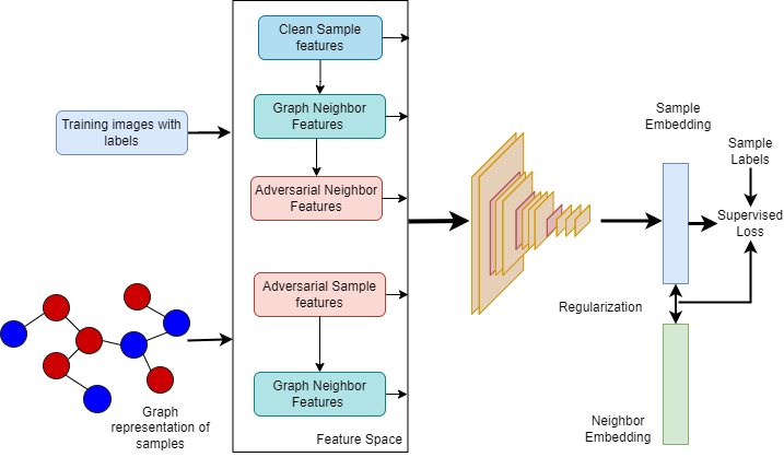
Figure 1: GReAT framework.

The feature space encompasses both the labeled original training samples and the adversarial examples that are created through adversarial regularization and neighbor similarities. This feature space is crucial for identifying the nearest-neighbor samples. When we feed a batch of input samples to the neural network, it includes not only the original samples but also their corresponding neighbors. In the final layer of the neural network, we derive a sample embedding for each of these samples. The training objective for regularization includes two components: the supervised loss and the label propagation loss, which accounts for neighbor-related loss. In other words, it considers the impact of neighbors on the overall training objective.

$$\mathcal{L}_{GReAT}=\mathcal{L}_{adv}+\lambda\mathcal{L}_{N},$$ (7)

where $\mathcal{L}_{adv}$ represents the supervised loss from training labels of clean and adversarially perturbed samples, and $\mathcal{L}_{N}$ represents the neighbor loss, which includes the loss from the clean training samples and adversarially perturbed samples.

We consider similar instances as neighbors of sample $\bm{x}$ in the graph regularized semi-supervised learning case. In our case, we consider an adversarial example, $\bm{x^{\prime}}$, in addition to a neighbor of sample $\bm{x}$. Next, we extend Eq. 6 by including adversarial and adversarial neighbor losses as new regularizer terms. Formally, the unpacked form of Eq.  7 is:

$$\begin{split}\mathcal{L}_{GReAT}(\Theta)=&\sum_{i=1}^{L}\ell(\theta,\bm{x}_{i},y_{i})\\ &+\alpha_{11}\sum_{i=1}^{L}\ell_{N}(y_{i},x_{i},\textsf{N}(x_{i}))\\ &+\alpha_{22}\sum_{i=1}^{L}\ell_{N}(y_{i},x^{\prime}_{i},\textsf{N}(x^{\prime}_{i}))\\ &+\alpha_{3}\sum_{i=1}^{L}\ell(\theta,\textsf{N}_{adv}(x_{i}),y_{i}),\end{split}$$ (8)

In the above equation, $\textsf{N}(\bm{x})$ represents neighbors of sample $\bm{x}$. The neighbors could be clean or adversarially perturbed samples. Thus, $\textsf{N}(\bm{x^{\prime}})$ represents the neighbors of adversarial example $\bm{x^{\prime}}$. Its neighbors could be clean samples and adversarial examples. Specifically, $\textsf{N}_{adv}(\bm{x})$ represents the adversarial neighbor of the sample $\bm{x}$. The adversarial neighbors have the same label as the original sample $\bm{x}$ similar to the standard adversarial training.

We obtain adversarial examples using the FGSM, ⁹, and PGD, ³⁷, methods. Note that the $\alpha_{11},\alpha_{22},\alpha_{3}$ hyperparameters determine the contributions of different neighborhood types, which are shown in Fig. 6 as sub-graph types. The $\alpha$ terms can be tuned according to the performance on clean and adversarially perturbed testing inputs. Furthermore, a detailed explanation of the embedding of neighbor nodes and graph construction between clean and adversarial samples is shown in Section 3.2.

3.1 Related Previous Methods

Creating graph embeddings using Deep Neural Networks (DNNs) is a well-known method, ³⁸. Furthermore, the propagation of unlabeled graph embeddings using transductive methods, ^{31, 5}, are efficient and well studied. Neural Graph Machines (NGMs), ⁴¹, are a commonly used example of label propagation and graph embeddings, along with supervised learning. The proposed training objective takes advantage of these frameworks and provides more robust image classifiers. Therefore, the training objective can be considered a combination of nonlinear label propagation and a graph-regularized version of adversarial training.

3.2 Graph Construction

We use a pre-trained model, DenseNet121, ⁴³, to generate image embeddings as a feature extractor. The pre-trained model has weights obtained by training on ImageNet. The pre-trained model is more complex than the model we use to train and test the proposed regularization algorithm in our simulations. Numerous studies show that complex DNNs are better feature extractors than shallow networks, ^{44, 45}. Another significant advantage of using larger pre-trained models to obtain embeddings is to reduce computational costs. The process of creating embeddings is illustrated in Fig. 2.

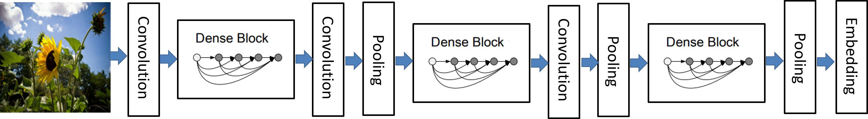
Figure 2: Densenet121 for creating image embeddings.

Generating appropriate inputs to the neural network plays a significant role in yielding correct predictions. As noted above, we use a pre-trained DL model to create node embeddings. We generate embeddings of clean samples and adversarial examples to obtain the neighborhood relationship between clean and adversarially perturbed examples. The overall graph construction process is shown in Fig. 3. Similarly, one-dimensional embedding is a crucial process for measuring sample similarities. Since the size of the embeddings is the same, we can visualize clean and adversarial samples in the embedding space using the ⁴⁶ t-distributed stochastic neighbor embedding (t-SNE) method.

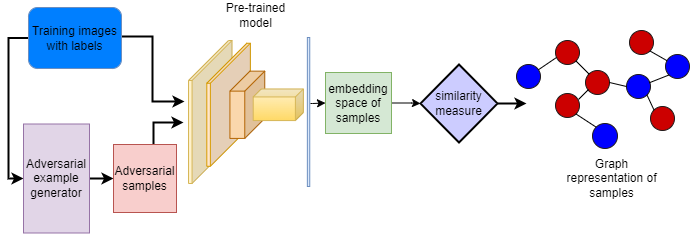
Figure 3: Densenet121 for creating image embeddings.

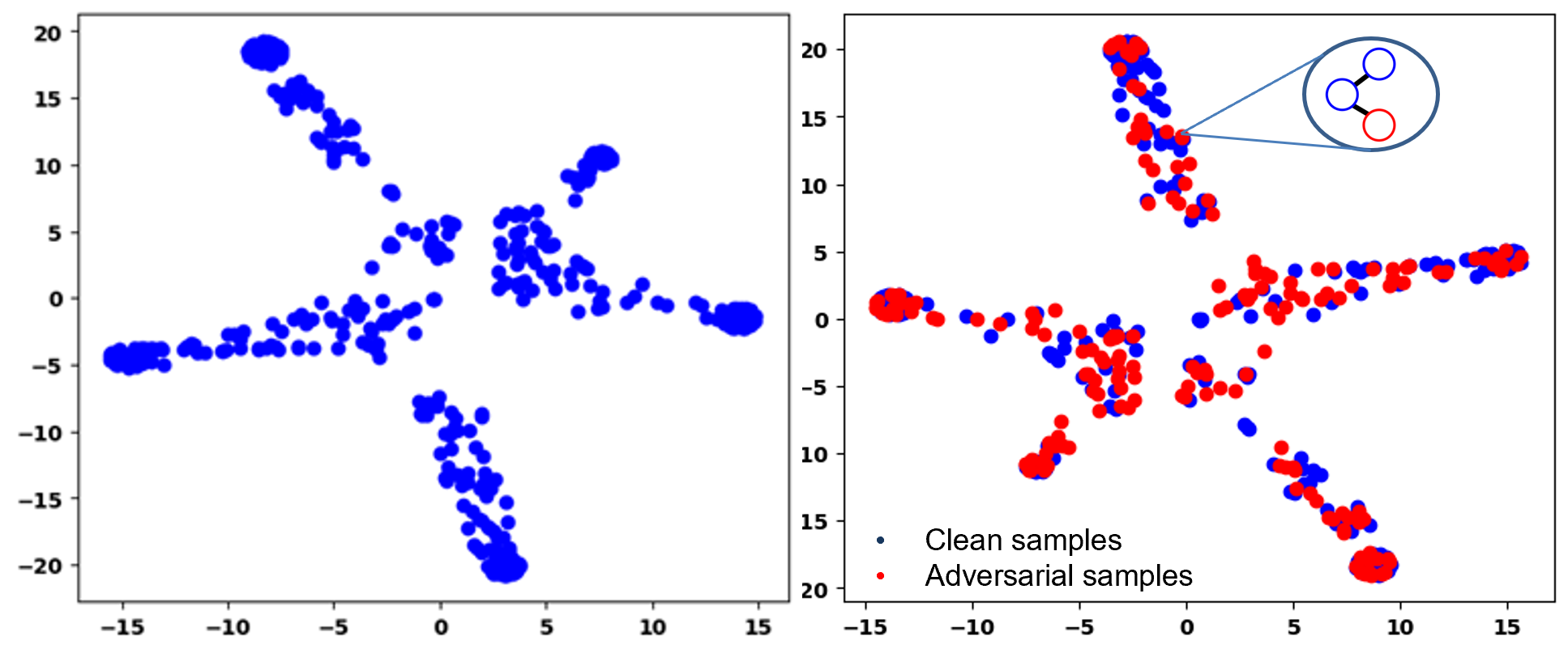
Figure 4: Samples in embedding space. The left figure represents all the samples in the validation data set. The right figure shows some clean samples and their adversarial neighbors.

In Figure 4, we utilize t-SNE (t-Distributed Stochastic Neighbor Embedding) to create a visual representation of the validation data set obtained from TensorFlow’s flower dataset. The primary purpose of this visualization is to provide insight into the distribution and relationships among the data points.The left panel of the figure is dedicated to displaying all the samples that constitute the validation data set. It is important to note that this data set encompasses samples belonging to five distinct classes. Each class represents a specific category or type of data within the dataset, and the samples within each class share certain common characteristics or features.

By visually representing the data set using t-SNE, we aim to reduce the dimensionality of the data while preserving its inherent structure and relationships. This reduction in dimensionality allows us to plot the data points in a two-dimensional space, making it easier to discern patterns, clusters, and similarities among the samples. Visualization is a valuable tool for gaining a deeper understanding of how the different classes are distributed and how they relate to each other within the validation data set. The figure panel on the right shows how adversarial examples are distributed around clean samples. The visualization of the embeddings highlights a strong connection between individual samples and their respective neighbors, effectively distinguishing between various classes.We use the strong neighborhood connections to learn better and create more robust models. Consequently, we use these node embeddings as input features to the neural network by creating an adjacency embedding matrix, as shown in Fig. 5. In particular, we use the label propagation method, ⁶, to propagate the information from the labeled data points to the unlabeled instances, which improves the model’s performance on both clean and adversarial examples.

Sample sub-graph of training instances are shown in Fig. 5. These examples might be labeled or unlabeled since we generate embeddings for each sample and create the graph based on the similarity between embeddings. A visual example of a sub-graph is demonstrated in Fig. 6. Three examples of sub-graph types are shown. The first column of the figure shows labeled samples. The second and third columns show the labeled samples’ two most similar neighbors. We associate these samples and their neighbors with the sub-graph examples, as noted in Fig. 5. For instance, the first row of images in Fig. 6 represents Fig. 5-D, since the labeled sample is clean and its first and second neighbors are adversarially perturbed samples. The second row of Fig. 6 represents Fig. 5-F, since the labeled sample is adversarially perturbed and its neighbors are one clean sample and one adversarially perturbed sample. Finally, the third row represents Fig. 5-C, since the labeled instance is clean and its neighbors are clean and adversarially perturbed samples. However, a labeled sample may have one neighbor or none, forinstance, if the similarity measure of embeddings cannot pass the similarity threshold. In that case, the labeled sample goes through the neural network as regular input without graph regularization.

Figure 5: A: A sample with two neighbors showing their sub-graph and feature inputs. Blue nodes represent clean samples, and red nodes represent adversarially perturbed samples. B,C,D,E,F, and G show how clean samples and adversarial examples may link on the graph structure.

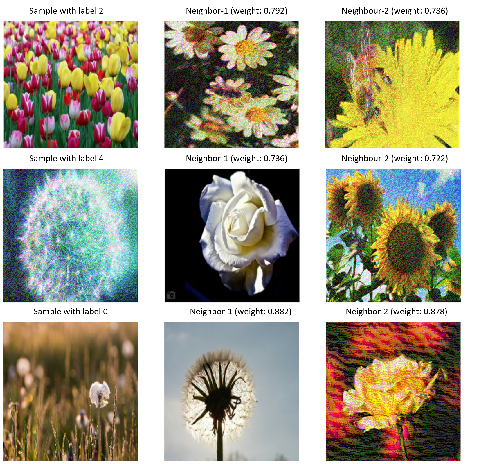
Figure 6: From left to right: labeled sample, the first neighbour and the second neighbour. The samples are taken from Tensorflow’s flowers data set.

3.3 Optimization

The training process begins with a minibatch of samples and their edges. Instead of using all available data at once, the training process randomly selects a subset of edges for each iteration. This helps introduce randomness and variability into the training process, which benefits the learning process. Additionally, to further improve the training process, selected edges are chosen from a nearby region to increase the likelihood of some edges. This can help reduce noise and speed up the learning process. The Stochastic Gradient Descent (SGD) algorithm updates the network weights utilizing the cross-entropy loss function.

Note that the overall open form of the cost function in the following is equivalent to Eq. 6. The cost function incorporates the cost of supervised loss from labeled clean and labeled adversarial samples and neighbor losses. That is, the cost includes different neighbor types/edges, as shown in Fig. 5. Formally,

$$\begin{split}\mathcal{L}_{GReAT}(\Theta)=&\sum_{i=1}^{L}\ell(\theta,\bm{x}_{i},y_{i})+\sum_{i=1}^{L}\ell(\theta,\bm{x^{\prime}}_{i},y_{i}),\\ &+\lambda\Biggr{[}\alpha_{11}\sum_{i=1}^{L}w_{a}\textsf{D}(g_{\theta}(x_{i}),\textsf{N}(g_{\theta}(x_{i})))\\ &+\alpha_{12}\sum_{i=1}^{L}w_{b}\textsf{D}(g_{\theta}(x_{i}),\textsf{N}(g_{\theta}(x^{\prime}_{i})))\\ &+\alpha_{21}\sum_{i=1}^{L}w_{c}\textsf{D}(g_{\theta}(x^{\prime}_{i}),\textsf{N}(g_{\theta}(x_{i})))\\ &+\alpha_{22}\sum_{i=1}^{L}w_{d}\textsf{D}(g_{\theta}(x^{\prime}_{i}),\textsf{N}(g_{\theta}(x^{\prime}_{i})))\Biggr{]},\end{split}$$ (9)

where $w_{a},w_{b},w_{c},w_{d}$ represent the similarity weights between the samples and their neighbors calculated by cosine similarity measurement.

The similarity weights are (possibly) unique for each sample and its neighbors, with a range of zero to one. A sample and neighbor candidate are dissimilar if the similarity weight is near zero. For calculating the neighbor loss, we use D as it represents the distance between a sample and its neighbor, where we use the norms $L_{1}$ and $L_{2}$ as distance metrics for calculating the neighbor distance. The hyperparameters $\alpha_{11},\alpha_{12},\alpha_{21}$ and $\alpha_{22}$ control the contributions of the different types of edges. For simulations, we set all $\alpha$s as one to include all edges in the training. The new objective function makes SGD possible with clean and adversarial samples and their neighbors in mini-batch training.

3.4 Complexity Analysis

The proposed method incorporates graph regularization into its training process, applying it to both labeled and unlabeled data instances within the graph, which includes benign and adversarial examples. The computational complexity of each training epoch is dependent on the number of edges in the graph, denoted as $E_{c}$. To elucidate the complexity of the training, we can express it as $O(count(E_{c}))$. It is important to note that the quantity $E_{c}$ is directly proportional to several factors. Firstly, it scales with the number of neighboring data points taken into consideration, signifying that more neighbors will increase the complexity. Second, it is influenced by a parameter that determines the selection of the most similar neighbors, further impacting the computational load. Moreover, the step size used for adversarial regularization is tied to $E_{c}$.

For instance, if we opt for a single-step adversarial regularization method like FGSM, each clear example will have only one adversarial neighbor. However, when employing a multi-step adversarial regularization approach, such as PGD, the number of edges substantially increases, as adversarial examples are generated at each step. This type of PGD-based adversarial regularization tends to enhance the model’s robustness compared to FGSM regularization. Nevertheless, it introduces a trade-off between robustness and training time. Training a model with PGD regularization demands more computational resources because of the increase in the number of edges and samples involved. This trade-off is essential when choosing the appropriate adversarial regularization method for a given application. For our simulations, we used FGSM to create adversarial examples for training and testing stages to reduce computational time.

4 Experiments

We conducted experiments to show the performance of the proposed GReAT method. Each experiment is carried out on clean data sets with a fixed number of epochs and training steps. The typical hyperparameters are fixed to ensure fair comparisons with other state-of-the-art methods. The base CNN model is trained and then regularized with the proposed loss function. We use the copy of the base model to obtain the regularized model each time to preserve the original base model. Once the models are trained, we test each model on the same clean and adversarially perturbed test data to measure the generalization and robustness performances.

4.1 Datasets

The CIFAR10, ³⁵, and flowers, ³⁴, datasets are used to evaluate the methods. The Cifar10 dataset consists of 60,000 images with ten classes, and each class contains a fixed size of $32\times 32$ three-channel RGB images. The flowers dataset contains 3,670 images with five classes, each containing high-resolution RGB images. The image sizes are not fixed in the flowers dataset. Resizing is, therefore, required as one of the pre-processing steps. The image distributions of each class are balanced for both data sets. We split the dataset 80%-10%-10%, as train-validation-test data sets, respectively. In the simulations, we reduce the training set to 20%, and 50%, to observe the model performances with fewer labeled samples.

4.2 Pre-processing Steps

A few essential pre-processing steps are required to prepare the batches for training. After creating image embeddings, we measure the similarity between each embedding and create training batches based on this similarity metric.

4.2.1 Similarity measure

Identifying the closest neighbors for a given sample requires the measurement of similarity amongst the embeddings. Various metrics are available, including Euclidean distance, cosine similarity, and Structural Similarity Index Measure (SSIM). We have opted for cosine similarity due to its proven effectiveness in quantifying the similarity of image embeddings within a multidimensional space. Formally defined, the cosine similarity of two vectors can be expressed as follows:

$$Cos(x_{i},x_{j})=\frac{x_{i}\cdot x_{j}}{\lVert x_{i}\rVert*\lVert x_{j}\rVert}.$$ (10)

The similarity weights are between 0 and 1, depending on the angle between the two vectors. Two overlapping embeddings have weight 1 when the angle between the two embeddings is zero. Conversely, if two embedding vectors are orthogonal, they are dissimilar, and the similarity weight is zero. Once all similarity weights are calculated, the most similar neighbors are identified as candidates for regularization. We pre-define a similarity threshold to consider those neighbors. Embeddings that fall under the threshold are not considered as neighboring candidates on the graph.

4.2.2 Training batches

Once the graph structure is created with clean samples and adversarial examples, we generate training batches that are fed into the neural network model. Each training batch consists of samples, their neighbors, and adversarial neighbors. The number of neighbors is predetermined, although other strategies can be utilized. In our simulations, we pick the number of neighbors as two.

4.3 Network

The base training model consists of four convolution layers and max-pooling layers. Dropout and batch normalization layers in the base model are deployed to minimize overfitting. We finalize the base model with fully connected and soft-max layers. The Adam optimizer with a 0.001 learning rate is utilized.

4.4 Results

First, we evaluate accuracy against attack strength by adjusting the magnitude of attack perturbation, providing insights into model performance across diverse attack intensities. Subsequently, experiments are conducted on both clean and adversarially perturbed datasets to gauge model generalization and robustness. We set the perturbation magnitude to 0.2 in these experiments and employ the FGSM attack method.

4.4.1 Results on Flowers Data Set

The above-mentioned flower dataset comprises high-resolution images. The performance of the proposed method, along with other state-of-the-art techniques on the clean dataset, is summarized in Table 1. Similarly, results for the adversarially perturbed dataset are presented in Table 2.

Table 1: Clean Accuracy Results for Flowers Data Set

Model Accuracy
	train set(%)	Base	NSL	AT	$GREAT_{adv}$	GREAT
	20%	0.548	0.553	0.525	0.207	0.550
	50%	0.564	0.608	0.575	0.245	0.659
	80%	0.597	0.613	0.583	0.277	0.671

Table 1 indicates that the NSL approach, ⁴¹, yields significantly better performance. This is largely due to its training on clean samples and their respective neighbors. For a comprehensive evaluation, we introduced $GReAT_{adv}$, which trains only adversarial samples and their neighbors to assess the impact of adversarial regularization. Given its exclusive focus on adversarial samples during training, this model faces challenges when tested on clean datasets. However, the proposed GReAT method consistently yields positive results.

Table 2: Robust Accuracy Results for Flowers Data Set

Attack Norm	train set(%)	Model Accuracy
		Base	NSL	AT	$GReAT_{adv}$	GReAT
L2	20%	0.011	0.011	0.450	0.836	0.605
	50%	0.014	0.024	0.496	0.854	0.647
	80%	0.016	0.063	0.526	0.891	0.668
Linf	20%	0.001	0.000	0.727	0.924	0.883
	50%	0.002	0.001	0.753	0.942	0.892
	80%	0.005	0.005	0.819	0.968	0.931

Finally, the models were evaluated using adversarially perturbed test data from the flowers data set, and the results are shown in Table 2. As the table shows, models not trained on adversarial examples, particularly the base model, exhibit diminished performance. Although the NSL model is trained only on clean samples, it still exhibits some robustness to adversarially perturbed test samples. The proposed GREAT model outperforms the other models and provides a balanced result for clean and adversarially perturbed testing data. $GReAT_{adv}$ gives the highest accuracy for perturbed test samples. This experiment shows how graph regularization with adversarial training is effective on both adversarially perturbed and clean testing samples.

4.4.2 Accuracy vs attack strength

We evaluate the robustness of the proposed methods by adjusting the step size of the perturbations, which provides insights into the model performance under varying attack strengths. As illustrated in Fig. 7, the accuracy of the base model declines sharply with increasing attack intensity. Although the model trained with standard adversarial training also exhibits a notable decrease in confidence, the proposed GReAT model consistently displays significant robustness, retaining its efficacy even under substantial perturbations.

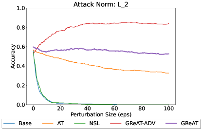
(a)

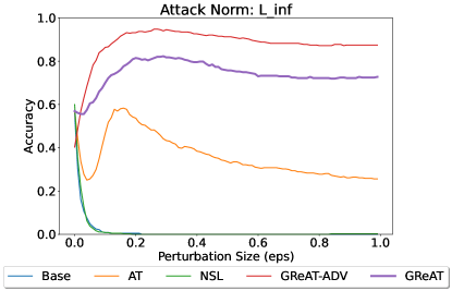
(b)

Figure 7: Robustness test with increasing perturbation size.

The perturbation sizes for adversarial training samples are $20$ for $L_{2}$ norm and $0.2$ for $L_{\infty}$ constrained models, respectively. As the figure shows, the models trained on adversarial examples exhibit peak performance around these specific training perturbation sizes ($\epsilon$). Ideally, we aim to train a model with varying perturbation sizes to enhance its robustness against adversarial attacks, given that attack perturbation sizes might differ from the training perturbation size. However, for the sake of simulation simplicity, we utilize only a single-step perturbation size for the model trainings.

4.4.3 Results on Cifar10 Data Set

Next, we evaluate the performance on the Cifar10 dataset, which is made up of images with lower resolution with more classes and quantities. Tables 3 and 4 detail the performance on the clean and adversarially perturbed image datasets, respectively. The proposed GReAT methodology yields balanced results, indicating that GReAT demonstrates both generalization and robust performance. In stark contrast, alternative methodologies are significantly impacted by adversarial attacks. These simulation results underscore that regularizing the deep learning model with both benign and adversarial examples results in improved generalization and robustness.

Table 3: Clean Accuracy Results for Cifar10 Data Set.

Model Accuracy
	train set(%)	Base	NSL	AT	$GReAT_{adv}$	GReAT
	20%	0.522	0.523	0.296	0.227	0.560
	50%	0.612	0.648	0.437	0.285	0.649
	80%	0.701	0.713	0.688	0.327	0.731

Compared to other methods, the proposed method shows outstanding performance on the benign testing set. This is because more training data and classes provide more underlying information between classes with graph regularization.

Table 4: Robust Accuracy Results for Cifar10 Data Set.

Attack Norm	train set(%)	Robust Accuracy
		Base	NSL	AT	$GReAT_{adv}$	GReAT
L2	20%	0.121	0.161	0.343	0.576	0.535
	50%	0.090	0.172	0.367	0.684	0.587
	80%	0.135	0.191	0.385	0.721	0.648
Linf	20%	0.003	0.071	0.415	0.699	0.613
	50%	0.004	0.079	0.517	0.720	0.646
	80%	0.004	0.105	0.570	0.744	0.668

Table 4 provides the performance of each model on adversarially perturbed testing data. As detailed in the table, the proposed method provides superior results to the NSL and standard adversarial training models. We observe similar results for $GReAT_{adv}$ in the Cifar10 data set, which shows the learning ability of GReAT over adversarial deceptive perturbations.

5 Conclusion

In this paper, we have presented a Graph Regularized Adversarial Training Method (GReAT), designed to enhance the robustness of classifiers. By leveraging classical adversarial training, the graph regularization technique enhances the robustness of deep learning classifiers. This technique employs graph-based constraints to regularize the training process, thereby bolstering the model’s capacity to withstand adversarial attacks. Integrating these constraints enables the model to learn more robust features and be less prone to manipulation via adversarial examples. This strategy has demonstrated significant potential in enhancing the robustness and generalization of deep learning classifiers, indicating that it could be a valuable tool in adversarial training.

References

- Krizhevsky et al. [2012] Alex Krizhevsky, Ilya Sutskever, and Geoffrey E Hinton. Imagenet classification with deep convolutional neural networks. Advances in neural information processing systems, 25:1097–1105, 2012.
- Liang and Hu [2015] Ming Liang and Xiaolin Hu. Recurrent convolutional neural network for object recognition. In Proceedings of the IEEE conference on computer vision and pattern recognition, pages 3367–3375, 2015.
- Goodfellow et al. [2020] Ian Goodfellow, Jean Pouget-Abadie, Mehdi Mirza, Bing Xu, David Warde-Farley, Sherjil Ozair, Aaron Courville, and Yoshua Bengio. Generative adversarial networks. Communications of the ACM, 63(11):139–144, 2020.
- Bengio et al. [2006] Yoshua Bengio, Olivier Delalleau, and Nicolas Le Roux. Label Propagation and Quadratic Criterion. Semi-Supervised Learning, pages 193–216, January 2006.
- Yang et al. [2016] Zhilin Yang, William W. Cohen, and Ruslan Salakhutdinov. Revisiting Semi-Supervised Learning with Graph Embeddings, May 2016. URL http://arxiv.org/abs/1603.08861. arXiv:1603.08861 [cs].
- Lee [2013] Dong-Hyun Lee. Pseudo-Label : The Simple and Efficient Semi-Supervised Learning Method for Deep Neural Networks. ICML 2013 Workshop : Challenges in Representation Learning (WREPL), July 2013.
- Joachims [1999] Thorsten Joachims. Transductive inference for text classification using support vector machines. In ICML ’99: Proceedings of the Sixteenth International Conference on Machine Learning, pages 200–209, San Francisco, CA, USA, 1999. Morgan Kaufmann Publishers Inc. ISBN 1-55860-612-2.
- Amini et al. [2022] Massih-Reza Amini, Vasilii Feofanov, Loic Pauletto, Emilie Devijver, and Yury Maximov. Self-training: A survey, 2022. URL https://arxiv.org/abs/2202.12040.
- Goodfellow et al. [2015] Ian Goodfellow, Jonathon Shlens, and Christian Szegedy. Explaining and harnessing adversarial examples. In International Conference on Learning Representations, 2015. URL http://arxiv.org/abs/1412.6572.
- Carlini and Wagner [2017a] Nicholas Carlini and David Wagner. Towards evaluating the robustness of neural networks. In 2017 IEEE Symposium on Security and Privacy (SP), pages 39–57, 2017a. doi: 10.1109/SP.2017.49.
- Nguyen et al. [2015] Anh Nguyen, Jason Yosinski, and Jeff Clune. Deep neural networks are easily fooled: High confidence predictions for unrecognizable images, 2015.
- Szegedy et al. [2014] Christian Szegedy, Wojciech Zaremba, Ilya Sutskever, Joan Bruna, Dumitru Erhan, Ian Goodfellow, and Rob Fergus. Intriguing properties of neural networks, 2014.
- Biggio and Roli [2018] Battista Biggio and Fabio Roli. Wild patterns: Ten years after the rise of adversarial machine learning. Pattern Recognition, 84:317–331, Dec 2018. ISSN 0031-3203. doi: 10.1016/j.patcog.2018.07.023. URL http://dx.doi.org/10.1016/j.patcog.2018.07.023.
- Moosavi-Dezfooli et al. [2016] Seyed-Mohsen Moosavi-Dezfooli, Alhussein Fawzi, and Pascal Frossard. Deepfool: a simple and accurate method to fool deep neural networks, 2016.
- Sharif et al. [2016] Mahmood Sharif, Sruti Bhagavatula, Lujo Bauer, and Michael K. Reiter. Accessorize to a crime: Real and stealthy attacks on state-of-the-art face recognition. In Proceedings of the 2016 ACM SIGSAC Conference on Computer and Communications Security, CCS ’16, page 1528–1540, New York, NY, USA, 2016. Association for Computing Machinery. ISBN 9781450341394. doi: 10.1145/2976749.2978392. URL https://doi.org/10.1145/2976749.2978392.
- Kurakin et al. [2016a] Alexey Kurakin, Ian J. Goodfellow, and Samy Bengio. Adversarial examples in the physical world. CoRR, abs/1607.02533, 2016a. URL http://arxiv.org/abs/1607.02533.
- Eykholt et al. [2018] Kevin Eykholt, Ivan Evtimov, Earlence Fernandes, Bo Li, Amir Rahmati, Chaowei Xiao, Atul Prakash, Tadayoshi Kohno, and Dawn Song. Robust physical-world attacks on deep learning models, 2018.
- Bayram and Barner [2022] Samet Bayram and Kenneth Barner. A black-box attack on optical character recognition systems, 2022. URL https://arxiv.org/abs/2208.14302.
- Madry et al. [2019] Aleksander Madry, Aleksandar Makelov, Ludwig Schmidt, Dimitris Tsipras, and Adrian Vladu. Towards deep learning models resistant to adversarial attacks, 2019.
- Carlini and Wagner [2017b] Nicholas Carlini and David Wagner. Towards evaluating the robustness of neural networks. In 2017 ieee symposium on security and privacy (sp), pages 39–57. IEEE, 2017b.
- Kurakin et al. [2016b] Alexey Kurakin, Ian Goodfellow, Samy Bengio, et al. Adversarial examples in the physical world, 2016b.
- Papernot et al. [2016a] Nicolas Papernot, Patrick McDaniel, Somesh Jha, Matt Fredrikson, Z Berkay Celik, and Ananthram Swami. The limitations of deep learning in adversarial settings. In 2016 IEEE European symposium on security and privacy (EuroS&P), pages 372–387. IEEE, 2016a.
- Tramèr et al. [2017] Florian Tramèr, Nicolas Papernot, Ian Goodfellow, Dan Boneh, and Patrick McDaniel. The space of transferable adversarial examples, 2017.
- Xie et al. [2019] Cihang Xie, Yuxin Wu, Laurens van der Maaten, Alan L Yuille, and Kaiming He. Feature denoising for improving adversarial robustness. In Proceedings of the IEEE/CVF Conference on Computer Vision and Pattern Recognition, pages 501–509, 2019.
- Bafna et al. [2018] Mitali Bafna, Jack Murtagh, and Nikhil Vyas. Thwarting adversarial examples: An -robustsparse fourier transform. arXiv preprint arXiv:1812.05013, 2018.
- Xie et al. [2017] Cihang Xie, Jianyu Wang, Zhishuai Zhang, Zhou Ren, and Alan Yuille. Mitigating adversarial effects through randomization. arXiv preprint arXiv:1711.01991, 2017.
- Wang et al. [2018] Bao Wang, Alex T Lin, Wei Zhu, Penghang Yin, Andrea L Bertozzi, and Stanley J Osher. Adversarial defense via data dependent activation function and total variation minimization. arXiv preprint arXiv:1809.08516, 2018.
- Papernot et al. [2016b] Nicolas Papernot, Patrick McDaniel, Xi Wu, Somesh Jha, and Ananthram Swami. Distillation as a defense to adversarial perturbations against deep neural networks. In 2016 IEEE symposium on security and privacy (SP), pages 582–597. IEEE, 2016b.
- Chen et al. [2019] Hao-Yun Chen, Jhao-Hong Liang, Shih-Chieh Chang, Jia-Yu Pan, Yu-Ting Chen, Wei Wei, and Da-Cheng Juan. Improving adversarial robustness via guided complement entropy. In Proceedings of the IEEE/CVF International Conference on Computer Vision, pages 4881–4889, 2019.
- Zhou et al. [2005] Dengyong Zhou, Jiayuan Huang, and Bernhard Schölkopf. Learning from labeled and unlabeled data on a directed graph. In Proceedings of the 22nd international conference on Machine learning - ICML ’05, pages 1036–1043, Bonn, Germany, 2005. ACM Press. ISBN 978-1-59593-180-1. doi: 10.1145/1102351.1102482. URL http://portal.acm.org/citation.cfm?doid=1102351.1102482.
- Zhu et al. [2005] Xiaojin Zhu, John Lafferty, and Ronald Rosenfeld. Semi-Supervised Learning with Graphs. PhD thesis, Carnegie Mellon University, USA, 2005. AAI3179046.
- Belkin et al. [2006] Mikhail Belkin, Partha Niyogi, and Vikas Sindhwani. Manifold Regularization: A Geometric Framework for Learning from Labeled and Unlabeled Examples. Journal of Machine Learning Research, 7(85):2399–2434, 2006. ISSN 1533-7928. URL http://jmlr.org/papers/v7/belkin06a.html.
- Carmon et al. [2019] Yair Carmon, Aditi Raghunathan, Ludwig Schmidt, John C Duchi, and Percy S Liang. Unlabeled Data Improves Adversarial Robustness. In Advances in Neural Information Processing Systems, volume 32. Curran Associates, Inc., 2019.
- TensorFlow [2019] TensorFlow. Flowers, jan 2019. URL http://download.tensorflow.org/example-images/flower-photos.tgz.
- Krizhevsky et al. [2009a] Alex Krizhevsky, Vinod Nair, and Geoffrey Hinton. Cifar-10 (canadian institute for advanced research). 2009a. URL http://www.cs.toronto.edu/~kriz/cifar.html.
- Ren et al. [2020] Kui Ren, Tianhang Zheng, Zhan Qin, and Xue Liu. Adversarial attacks and defenses in deep learning. Engineering, 6(3):346–360, 2020.
- Madry et al. [2017] Aleksander Madry, Aleksandar Makelov, Ludwig Schmidt, Dimitris Tsipras, and Adrian Vladu. Towards deep learning models resistant to adversarial attacks. arXiv preprint arXiv:1706.06083, 2017.
- Weston et al. [2008] Jason Weston, Frédéric Ratle, and Ronan Collobert. Deep learning via semi-supervised embedding. In Proceedings of the 25th International Conference on Machine Learning, ICML ’08, page 1168–1175, New York, NY, USA, 2008. Association for Computing Machinery. ISBN 9781605582054. doi: 10.1145/1390156.1390303. URL https://doi.org/10.1145/1390156.1390303.
- Agarwal et al. [2009] Nitin Agarwal, Huan Liu, Sudheendra Murthy, Arunabha Sen, and Xufei Wang. A Social Identity Approach to Identify Familiar Strangers in a Social Network. Proceedings of the International AAAI Conference on Web and Social Media, 3(1):2–9, March 2009. ISSN 2334-0770. URL https://ojs.aaai.org/index.php/ICWSM/article/view/13946. Number: 1.
- Jacob et al. [2014] Yann Jacob, Ludovic Denoyer, and Patrick Gallinari. Learning latent representations of nodes for classifying in heterogeneous social networks. In Proceedings of the 7th ACM international conference on Web search and data mining, pages 373–382, New York New York USA, February 2014. ACM. ISBN 978-1-4503-2351-2. doi: 10.1145/2556195.2556225. URL https://dl.acm.org/doi/10.1145/2556195.2556225.
- Bui et al. [2018] Thang D. Bui, Sujith Ravi, and Vivek Ramavajjala. Neural Graph Learning: Training Neural Networks Using Graphs. In Proceedings of the Eleventh ACM International Conference on Web Search and Data Mining, pages 64–71, Marina Del Rey CA USA, February 2018. ACM. ISBN 978-1-4503-5581-0. doi: 10.1145/3159652.3159731. URL https://dl.acm.org/doi/10.1145/3159652.3159731.
- Zhou et al. [2004] Dengyong Zhou, Olivier Bousquet, Thomas N Lal, Jason Weston, and Bernhard Schölkopf. Learning with Local and Global Consistency. page 8, 2004.
- Huang et al. [2016] Gao Huang, Zhuang Liu, Laurens van der Maaten, and Kilian Q. Weinberger. Densely connected convolutional networks, 2016. URL https://arxiv.org/abs/1608.06993.
- Krizhevsky et al. [2009b] Alex Krizhevsky, Geoffrey Hinton, et al. Learning multiple layers of features from tiny images. 2009b.
- Mhaskar et al. [2017] Hrushikesh Mhaskar, Qianli Liao, and Tomaso A. Poggio. When and why are deep networks better than shallow ones? In Satinder P. Singh and Shaul Markovitch, editors, AAAI, pages 2343–2349. AAAI Press, 2017. URL http://dblp.uni-trier.de/db/conf/aaai/aaai2017.htmlMhaskarLP17.
- van der Maaten and Hinton [2008] Laurens van der Maaten and Geoffrey Hinton. Visualizing data using t-SNE. Journal of Machine Learning Research, 9:2579–2605, 2008. URL http://www.jmlr.org/papers/v9/vandermaaten08a.html.