ZooPFL: Exploring Black-box Foundation Models for Personalized Federated Learning

Abstract

When personalized federated learning (FL) meets large foundation models, new challenges arise from various limitations in resources. In addition to typical limitations such as data, computation, and communication costs, access to the models is also often limited. This paper endeavors to solve both the challenges of limited resources and personalization. i.e., distribution shifts between clients. To do so, we propose a method named ZooPFL that uses Zeroth-Order Optimization for Personalized Federated Learning. ZooPFL avoids direct interference with the foundation models and instead learns to adapt its inputs through zeroth-order optimization. In addition, we employ simple yet effective linear projections to remap its predictions for personalization. To reduce the computation costs and enhance personalization, we propose input surgery to incorporate an auto-encoder with low-dimensional and client-specific embeddings. We provide theoretical support for ZooPFL to analyze its convergence. Extensive empirical experiments on computer vision and natural language processing tasks using popular foundation models demonstrate its effectiveness for FL on black-box foundation models.

Sec. 1 Introduction

In recent years, the growing emphasis on data privacy and security has led to the emergence of federated learning (FL) (Warnat-Herresthal et al., 2021; Chen & Chao, 2022; Chen et al., 2023b; Castiglia et al., 2023; Rodríguez-Barroso et al., 2023; Kuang et al., 2023). FL enables collaborative learning while safeguarding data privacy and security across distributed clients (Yang et al., 2019). However, FL faces two key challenges: limited resources and distribution shifts (Figure 1 (a, b)).

The rise of large foundation models (Bommasani et al., 2021) has amplified these challenges. The computational demands and communication costs associated with such models hinder the deployment of existing FL approaches (Figure 1a). Most of them require fine-tuning the models on every client. Moreover, foundation models, often proprietary (Van Dis et al., 2023; Sun et al., 2022), grant only black-box access, making FL resource-efficient applications a pressing research area.

Recent efforts in FL (Xu et al., 2023b; Zhao et al., 2023; Chen et al., 2023d; Li et al., 2023) have attempted to reduce the number of optimized parameters to minimize computational and communication costs. As illustrated in Figure 1 (c), existing methods use prompts (Liu et al., 2023) or adapters (Cai et al., 2022) to fine-tune foundation models (Xu et al., 2023b). Other approaches (Yurochkin et al., 2019; Liu et al., 2022) focus on limiting the number of communication rounds. All of them however depend on white-box access to the foundation models. On the other hand, distribution shifts are an additional challenge for FL since the data across clients is not necessarily i.i.d. (Li et al., 2020b; Vemulapalli et al., 2023) (Figure 1b). Directly aggregating information e.g., with FedAVG (McMahan et al., 2017) often results in slow convergence and poor performance in each client (Gao et al., 2022). Some methods have been designed to address the personalization of large foundation models (Li et al., 2021; Setayesh et al., 2023; Xu et al., 2023a). However, they cannot deal with black-box models. The method proposed in this paper is designed to cope with label shift, i.e. variations in the distribution of labels among clients (Figure 1b).

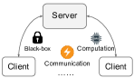
(a) Limited resources

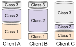
(b) Distribution shifts

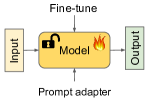
(c) Existing methods

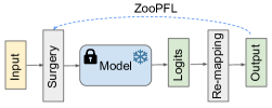
(d) Our proposed ZooPFL

Figure 1: ZooPFL addresses federated learning with foundation models while coping with limited resources in communication, computation, and model accessibility (a) and being robust to distribution shifts (b). Most existing methods rely on white-box model access (c). In contrast, ZooPFL is applicable to black-box models by using input surgery and semantic output re-mapping (d).

In this paper, we propose ZooPFL to cope with limited resources and personalization for federated learning and black-box foundation models. To cope with black-box models, ZooPFL proposes two strategies, input surgery and semantic re-mapping, and learning through zeroth-order optimization (ZOO). To reduce the computational costs of ZOO and share information among clients, we employ an auto-encoder with low embedding dimensions to represent transformations. For better personalization, the client-specific embeddings and semantic re-mapping are preserved by each client. Figure 1 (d) illustrates that our proposed method learns transformations on the inputs and mappings of the outputs through zeroth-order optimization (Liu et al., 2020; Wang et al., 2018; Lian et al., 2016). This bears similarities with model reprogramming  (Chen, 2022) and Reprogrammable-FL (Arif et al., 2023), but the latter is unsuitable for black-box models and personalization. To the best of our knowledge, our method is the first to achieve federated learning with large black-box models, a challenging setting that is becoming increasingly relevant to the real world.

In summary, our contributions are four-fold.

1. Scenario Exploration: We delve into the challenges posed by fully black-box foundation models in FL. Our contribution lies in understanding and navigating this complex scenario.

2. ZooPFL Framework: We introduce ZooPFL, a comprehensive solution tailored for FL in resource-constrained and personalized settings. This framework encompasses Input Surgery and Semantic Re-mapping. ZooPFL employs strategic input manipulations, leveraging dedicated embeddings, and employing zeroth-order optimization while it project outputs for specific task and personalization.

3. Theoretical Support: We provide formal theoretical support, enhancing ZooPFL’s credibility and offering insights into its workings.

4. Empirical Validation: ZooPFL is rigorously evaluated through computer vision and natural language processing experiments, demonstrating the effectiveness and versatility of ZooPFL.

Sec. 2 Related Work

Federated learning makes it possible to perform distributed multi-party computing without comprising privacy (Zhang et al., 2021; Voigt & Von dem Bussche, 2017; McMahan et al., 2017; Yang et al., 2019; Tariq et al., 2023; Wang et al., 2023a; So et al., 2023). When meeting non-iid data, common FL methods, e.g. FedAVG (McMahan et al., 2017) can suffer from low converge speed and terrible personalization performance (Sattler et al., 2019). Specific methods, e.g. FedProx (Li et al., 2020b) and FedBN (Li et al., 2021), are proposed for personalization while additional methods, e.g. (Chen & Chao, 2022; Gupta et al., 2022; Qu et al., 2022), also consideration generalization.

The above methods can fail when entering the era of large foundation models (Bommasani et al., 2021; Xing et al., 2023; Zhuang et al., 2023), due to novel issues, e.g. limited resources that make operations on the whole network impossible (Chen et al., 2022; 2023a; Ding et al., 2023). Recent work (e.g. FedPrompt (Zhao et al., 2023),PromptFL (Guo et al., 2023), pFedPG (Yang et al., 2023a), FwdLLM (Xu et al., 2023b)) were proposed to tune part of the whole network for efficiency. However, they all require access to foundation models, which can be impossible in reality.

In addition to data privacy, model privacy also raises attention (Mo et al., 2020), which means foundation models can be black-box models (Guidotti et al., 2018; Ljung, 2001). Little work paid attention to finetuning or optimizing in this field, but most related work focused on attacks (Yang et al., 2023b; c). One related work is FedZO (Fang et al., 2022) which utilized zero-order optimization (Ghadimi & Lan, 2013), but it did not consider utilizing large foundation models.

Model reprogramming (MR) (Tsai et al., 2020; Xu et al., 2023c; Chen, 2022) provides a similar solution to ZooPFL and it also focuses on coping with inputs and outputs. Reprogrammable-FL (Arif et al., 2023) adapted MR to the setting of differentially private federated learning. But it preserved local input transformations and shared output transformation layers, which were totally in contrast to ours. Table 1 provides a comprehensive comparison between existing methods and ours. For more detailed related work, please refer to section B.

Sec. 3 Methodology

In this section, we articulate our proposed ZooPFL. We begin with problem formulation in Sec. 3.1. Then, we show the motivation of designing ZooPFL in Sec. 3.2. Next, Sec. 3.3 introduces the details of our approach. Finally, Sec. 3.4 provides theoretical analysis.

Table 1: Comparisons of different methods.

Type	Method	Model scale	Model accessibility	Communication	Computation	Personalization
Base	FedAVG	Limited	White-box	Inefficient	High	Unsupported
	FedBN					Supported
Large model for FL	FedPrompt, FedCLIP	Unlimited	White-box	Efficient	Low	Supported
	PromptFL, pFedPG				High
Zero-order for FL	FwdLLM, BAFFLE	Unlimited	White-box	Efficient	Low	Supported
	FedZO	Limited
Model reprogramming	Reprogrammable-FL	Unlimited	White-box	Efficient	High	Supported
Black-box foundation FL	ZooPFL (Ours)	Unlimited	Black-box	Efficient	Low	Supported

3.1 Problem Formulation

We assume there are $n$ different clients $\{C_{1},\cdots,C_{n}\}$ in personalized federated learning scenarios. Each client $C_{i}$ has its own data $\mathcal{D}_{i}=\{\mathbf{x}_{i,j},y_{i,j}\}_{j=1}^{n_{i}}$ where $n_{i}$ means the number of data in the $i$th client. Data in different clients have different distributions, i.e. $P(\mathcal{D}_{i})\neq P(\mathcal{D}_{j})$. In the personalized FL setting, there exists the same black-box large foundation model in each client, $g$, which we know nothing inside and can only obtain logit outputs with fixed-size inputs. Our goal is to achieve personalized (i.e., satisfying) performance with black-box foundation models on each client by learning a significant transformation $s_{i}$ on inputs and a re-mapping $r_{i}$ on outputs without accessing $g$ for each client $\mathcal{D}_{i}$. Specifically, denote $\ell$ a loss function, the learning objective is:

$$\min_{s_{i},r_{i}}\frac{1}{n}\sum_{i=1}^{n}\frac{1}{n_{i}}\sum_{j=1}^{n_{i}}\ell(r_{i}(g(s_{i}(\mathbf{x}_{i,j}))),y_{i,j}).$$ (1)

3.2 Intuition

Input designs affect the performance of foundation models. Different representations with the same inputs can induce foundation models to make completely different predictions, which illustrates that adding interference or reconstructing inputs can be utilized for adaptation. However, most methods that add interference are performed at the sample level (White et al., 2023; Cao et al., 2023; Liu & Chilton, 2022; Arif et al., 2023; Zhou et al., 2022; Gal et al., 2022) , i.e. special design for each sample, that are unsuitable to exchange information among clients and cannot cope with unseen samples. Therefore, it is necessary to reconstruct samples via an auto-encoder to adapt input with unchanged dimensions for foundation models. The exchange of auto-encoder parameters can facilitate the sharing of input transformation information across different clients.

Semantic re-mapping generates more semantically meaningful logits. Although large foundation models have been trained on a huge amount of samples (Radford et al., 2021), there still exists some classes or situations that foundation models cannot cover (Wang et al., 2023b). However, these new scenarios or classes can be made of existing fundamental elements or similar to some existing categories, which means foundation models can be able to extract remarkable features. Considering layers between remarkable features and final logits as random projecting, re-mapping outputs with a simple linear layer can achieve acceptable performance similar to Huang et al. (2015).

Design logic. Since access to foundation models is restricted, we have to rely on zeroth-order optimization methods to train auto-encoders, which leads that directly operating on the outputs of auto-encoders with high dimensions can exhaust unaffordable computational costs. To reduce the costs, we fix decoders and compute differences on embedding with low dimensions. For better personalization, we preserve semantic re-mapping in clients. Specifically, we preserve a client-specific embedding, i.e., a simple one-dimensional vector, for each client, which can be concatenated with embedding to generate adapted inputs with personalized characteristics.

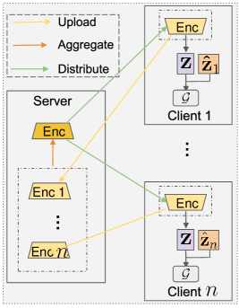
(a) Communication of server-client

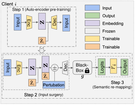
(b) Training process in client $i$

Figure 2: The framework of ZooPFL. Please note that communications occur during step 2.

3.3 ZooPFL

In this paper, we propose ZooPFL to learn input surgery and semantic re-mapping for black-box large foundation models in federated learning. ZooPFL aims to adapt inputs to models and project outputs to meaningful semantic space. ZooPFL mainly consists of three steps, namely, auto-encoder pre-training, input surgery, and semantic re-mapping. Figure 2 shows the pipeline of our approach, where Figure 2(a) describes the communications between clients and the server and Figure 2(b) provides details on how to perform training on a local client. The algorithm flow is in Appendix C.1.

The training process on a client is described as follows, where steps 2$\sim$3 are iterative.

1. Auto-encoder pre-training: this step directly utilizes inputs to pre-train the auto-encoder which then serves as the input surgery function.

2. Input surgery: this step only updates the encoder of auto-encoder and client-specific embeddings to transform the input consistent with the foundation model.

3. Semantic re-mapping: this step endeavors to re-map logits into meaningful semantic spaces with a simple linear projection.

Auto-encoder Pre-training.

Before input surgery and semantic re-mapping that are assisted by labels, ZooPFL firstly utilizes inputs of samples to pre-train auto-encoders for better initial understanding of client data and we will fix decoders in the next two steps. For client $C_{i}$, we denote $\hat{\mathbf{z}_{i}}$ as the $i$th client-specific embedding and $s_{i}=o_{i}\circ q_{i}$ where $q_{i}$ and $o_{i}$ represent the encoder and the decoder respectively. This step is unsupervised and each client utilizes MSE loss to train local $s_{i}$:

$$\ell_{MSE}=\mathbb{E}_{(\mathbf{x},y)\sim\mathbb{P}(\mathcal{D}_{i})}\left\|o_{i}([q_{i}(\mathbf{x}),\hat{\mathbf{z}_{i}}])-\mathbf{x}\right\|_{2}^{2},$$ (2)

where $[\cdot,\cdot]$ denotes the concatenation operation. The updated encoder and decoder of each client are then transmitted to the server. Similar to FedAVG (McMahan et al., 2017), the server aggregates the collected auto-encoders and distributes the aggregated one, $s$, to each client.

$$w(s)=\frac{1}{n}\sum_{i=1}^{n}w(s_{i}),$$ (3)

where $w(s)$ represent parameters of $s$. We assume that all clients contribute equally and participate in training. The above pre-training is iterative and we can obtain well-trained auto-encoders finally.

Input Surgery.

After pre-training, input surgery optimizes encoders, $q_{i}$, to transform inputs consistent with foundation models. This step only exchanges encoders of clients to share common knowledge while each client preserves a client-specific embedding to represent personalized knowledge. As shown in Figure 2, the foundation model, $g$, is black-box and the decoder is frozen. In the following, we elaborate on the whole training process in local clients.

In client $C_{i}$, an input $\mathbf{x}$ is first fed into the encoder $q_{i}$, generating an embedding vector $\mathbf{z}=q_{i}(\mathbf{x})$. Then we concatenate $\mathbf{z}$ with the client-specific embedding, $\hat{\mathbf{z}_{i}}$, and obtain the final embedding feature, $\tilde{\mathbf{z}}=[\mathbf{z},\hat{\mathbf{z}_{i}}]$, which is then sent to the decoder. Once processed by the decoder, we can obtain $\tilde{\mathbf{x}}=o_{i}(\tilde{\mathbf{z}})$ with the same dimension as $\mathbf{x}$, and then the adapted input, $\tilde{\mathbf{x}}$, goes through the foundation model and the re-mapping layer, which generates the final prediction, $\tilde{\mathbf{y}}$. We utilize the cross-entropy loss $\ell_{cls}$ to guide the optimization:

$$\ell_{1}=\mathbb{E}_{(\mathbf{x},y)\sim\mathbb{P}(\mathcal{D}_{i})}\ell_{cls}(r_{i}(g(o_{i}([q_{i}(\mathbf{x}),\hat{\mathbf{z}_{i}}])),y).$$ (4)

However, the above objective cannot be directly optimized using the standard stochastic gradient descent since the foundation model $g$ is frozen, preventing us from computing its gradient using back-propagation. We adopt the zeroth-order optimization method, specifically, the coordinate-wise gradient estimate (CGE), to learn $q_{i}$ and $\hat{\mathbf{z}_{i}}$ (Zhang et al., 2022; Tu et al., 2019; Liu et al., 2018; Lian et al., 2016; Ghadimi & Lan, 2013). To make the process clear and easy to understand, we freeze $r_{i}$ and view $o_{i}$, $g$, and $r_{i}$ as a whole module, $\mathcal{G}$, in this step.

Assume $\mathbf{z}\in\mathbb{R}^{d_{1}}$ and $\hat{\mathbf{z}_{i}}\in\mathbb{R}^{d_{2}}$. According to CGE, by adding a perturbation to $\tilde{\mathbf{z}}$, we obtain the new embedding and the corresponding classification loss,

$$\tilde{\mathbf{z}_{1}}=\tilde{\mathbf{z}}+\rho\mathbf{e}_{j},\ell_{\mathbf{x},1}=\ell_{cls}(r_{i}(g(o_{i}(\tilde{\mathbf{z}_{1}},y)))),$$ (5)

where $\mathbf{e}_{j}=(0,0,\cdots,1,0,0\cdots,0)\in\mathbb{R}^{d_{1}+d_{2}}$ denotes the $j$th elementary basic vector and $\rho$ is a hyperparameter that describes the extent of the perturbation. Similarly, we can obtain $\tilde{\mathbf{z}_{2}}$ and $\ell_{\mathbf{x},2}$.

$$\tilde{\mathbf{z}_{2}}=\tilde{\mathbf{z}}-\rho\mathbf{e}_{j},\ell_{\mathbf{x},2}=\ell_{cls}(r_{i}(g(o_{i}(\tilde{\mathbf{z}_{2}},y)))).$$ (6)

Then, we have the gradient of $\mathcal{G}$ w.r.t. $\tilde{\mathbf{z}}$ computed as:

$$\nabla_{\tilde{\mathbf{z}}}\mathcal{G}(\tilde{\mathbf{z}})=(\nabla_{\tilde{\mathbf{z}}}\mathcal{G}(\tilde{\mathbf{z}})_{1},\nabla_{\tilde{\mathbf{z}}}\mathcal{G}(\tilde{\mathbf{z}})_{2})\approx\sum_{i=1}^{d_{1}+d_{2}}\frac{\ell_{\mathbf{x},2}-\ell_{\mathbf{x},1}}{2\times\rho}\mathbf{e}_{j}.$$ (7)

For $\hat{\mathbf{z}_{i}}$, we directly update it with corresponding parts of $\nabla_{\tilde{\mathbf{z}}}\mathcal{G}(\tilde{\mathbf{z}})$ via a learning rate $\gamma_{2}$, $\hat{\mathbf{z}_{i}}^{new}=\hat{\mathbf{z}_{i}}-\gamma_{2}\times\nabla_{\tilde{\mathbf{z}}}\mathcal{G}(\tilde{\mathbf{z}})_{2}$ where $\nabla_{\tilde{\mathbf{z}}}\mathcal{G}(\tilde{\mathbf{z}})_{2}$ denotes the last $d_{2}$ dimensions of $\nabla_{\tilde{\mathbf{z}}}\mathcal{G}(\tilde{\mathbf{z}})$. For $\nabla_{\tilde{\mathbf{z}}}\mathcal{G}(\tilde{\mathbf{z}})_{1}$, we can update $q_{i}$ with the chain rule for differentiation.

$$\nabla_{q_{i}}\ell_{1}=\frac{d\tilde{\mathbf{z}}}{dq_{i}}\frac{d\mathcal{G}}{d\tilde{\mathbf{z}}}\approx\frac{d\mathbf{z}}{dq_{i}}\nabla_{\tilde{\mathbf{z}}}\mathcal{G}(\tilde{\mathbf{z}})_{1}\approx\frac{d\nabla_{\tilde{\mathbf{z}}}\mathcal{G}(\tilde{\mathbf{z}})_{1}\mathbf{z}}{dq_{i}}.$$ (8)

Finally, we can update the encoder, $w(q_{i}^{new})=w(q_{i})-\gamma_{1}\times\nabla_{q_{i}}\ell_{1}$. Once all clients have updated encoders, we can aggregate encoders in the server and then distribute the aggregated encoder:

$$w(q)=\frac{1}{n}\sum_{i=1}^{n}w(q_{i}^{new}).$$ (9)

Semantic Re-mapping.

In the last step, we train the encoder that enables the input consistent with foundation models. Here, we perform semantic re-mapping similar to Huang et al. (2015). This step only occurs in each client and no communication exists for simplicity and personalization. We view all parts before $r_{i}$ as a whole module, $\mathcal{F}$, with two functions, including extracting features and mapping extracted features to a random space and we freeze $\mathcal{F}$. These two functions correspond to artificial features and the first layer in (Huang et al., 2015) respectively and we only update $r_{i}$ corresponding to the second layer of ELM:

$$\ell_{2}=\mathbb{E}_{(\mathbf{x},y)\sim\mathbb{P}(\mathcal{D}_{i})}\ell_{cls}(r_{i}(\mathcal{F}(\mathbf{x})),y).$$ (10)

Since this part is behind $g$, $w(r_{i})$ can be updated directly.

Discussion.

We perform step 2 and step 3 iteratively. There also exist other zeroth-order optimization methods, e.g., the randomized gradient estimate (RGE) (Liu et al., 2020). However, the concrete implementation of zeroth-order optimization is not our focus and we thereby choose CGE for deterministic and stability (Liu et al., 2018). In this paper, we assume large foundation models exist on clients in the form of encrypted assets and we do not need to upload transformed inputs. Moreover, we do care about communication costs and GPU demands instead of training time in each client. To reduce training time in each client, some techniques, such as RGE, random selections on $\mathbf{e}_{j}$, reduction on $d_{1}+d_{2}$, etc., can be adopted and we leave this as our future work.

3.4 Theoretical Analysis

We present the convergence analysis of ZooPFL. There exist three parts to optimize during step 2 and step 3, including the parameters of the encoder ($\mathbf{\hat{u}}$), clients specific embeddings ($\mathbf{v}_{1,i}$), and semantic re-mapping layers ($\mathbf{v}_{2,i}$). Following Pillutla et al. (2022), we group parameters into two parts, i.e. $\mathbf{u}_{i}:=\mathbf{\hat{u}}\cup\mathbf{v}_{1,i}$, $\mathbf{v}_{i}:=\mathbf{v}_{2,i}$. Now we give the main conclusion with proofs in Appendix A.

Theorem 1.

Suppose assumptions 1, 2, 3, and 4 hold, and the learning rates in ZooPFL are chosen as $\gamma_{\mathbf{u}}=\eta/(L_{\mathbf{u}}\tau_{\mathbf{u}})$ and $\gamma_{\mathbf{v}}=\eta/(L_{\mathbf{v}}\tau_{\mathbf{v}})$, with

$$\eta\leq\textit{min}\left\{{1\over 24(1+\mu^{2})},\frac{m}{128\chi^{2}(n-m)},\sqrt{m\over\chi^{2}n}\right\}.$$ (11)

Then, right after the training of $T$ epochs, ignoring absolute constants, we have

$$\frac{1}{T}\sum_{t=0}^{T-1}\left(\frac{1}{L_{\mathbf{u}}}\mathbb{E}\left[\Delta_{\mathbf{u}}^{(t)}\right]+\frac{m}{nL_{\mathbf{v}}}\mathbb{E}\left[\Delta_{\mathbf{v}}^{(t)}\right]\right)\leq\frac{\Delta F_{0}}{\eta T}+\eta\sigma^{2}_{alt,1}+\eta^{2}\sigma^{2}_{alt,2}.$$ (12)

Corollary 1.

An optimal learning rate is:

$$\eta=\left(\frac{\Delta F_{0}}{T\sigma_{alt,1}^{2}}\right)^{1/2}\bigwedge\left(\frac{\Delta F_{0}^{2}}{T^{2}\sigma_{alt,2}^{2}}\right)^{1/3}\bigwedge\frac{1}{1+\mu^{2}}\bigwedge\frac{m}{\chi^{2}(n-m)}\bigwedge\sqrt{\frac{m}{\chi^{2}n}}.$$ (13)

We have, ignoring absolute constants,

$$\begin{aligned} &\frac{1}{T}\sum_{t=0}^{T-1}\left(\frac{1}{L_{\mathbf{u}}}\mathbb{E}\left[\Delta_{\mathbf{u}}^{{(t)}}\right]+\frac{m}{nL_{\mathbf{v}}}\mathbb{E}\left[\Delta_{\mathbf{v}}^{{(t)}}\right]\right)\leq\\ &\frac{(\Delta F_{0}\sigma_{alt,1}^{2})^{1/2}}{\sqrt{T}}+\frac{(\Delta F_{0}^{2}\sigma_{alt,2}^{2})^{1/3}}{T^{2/3}}+\frac{\Delta F_{0}}{T}\left(1+\mu^{2}+\chi^{2}(\frac{n}{m}-1)+\sqrt{\chi^{2}\frac{n}{m}}\right).\end{aligned}$$ (14)

The measure of convergence of Algorithm 1 is in terms of the weighted average of square norms of the gradients of loss function $\mathbb{E}\left[\Delta_{\mathbf{u}}^{{(t)}}\right]$ and $\mathbb{E}\left[\Delta_{\mathbf{v}}^{{(t)}}\right]$ through iterations from 1 to $T-1$, i.e. the left hand of equation 14. As the square norms of the gradients of loss function at the optimal solution is zero, whether or not these norms approach zero is a good criterion of the convergence. With this choice of optimal learning rate, it is clear from the right hand of equation 14 that our algorithm converges and the asymptotic convergence rate is $\mathbf{O}({1\over\sqrt{T}})$.

Sec. 4 Experiments

4.1 Setup

Table 2: Information of benchmarks.

Modality	Dataset	Samples	Classes	Clients	Selected Samples
CV	COVID-19	9,198	4	20	9,198
	APTOS	3,662	5	20	1,658
	Terra100	5,883	10	20	5,883
	Terra46	4,741	10	20	4,741
NLP	SST-2	67k	2	20	9,763
	COLA	8.5k	2	20	5,700
	Finanical	4,840	3	10	3,379
	Flipkart	205,053	3	20	3,048

Datasets and baselines. We evaluate ZooPFL on 8 popular classification benchmarks with two modalities including computer vision (CV) and natural language processing (NLP). The benchmarks are COVID-19 (Sait et al., 2020), APTOS (Karthik, 2019), Terra100 (Beery et al., 2018), Terra46 (Beery et al., 2018), SST-2 (Wang et al., 2019; Socher et al., 2013), COLA (Wang et al., 2019; Warstadt et al., 2019), Financial-phrasebank (Financial) (Malo et al., 2014), and Flipkart (Vaghani & Thummar, 2023). Brief information can be found in Table 2. We filter meaningless samples and select samples for global class balance. The concrete select strategies and more details can be found in section D.1 while data distributions can be found in section D.2. To our best knowledge, no other methods are proposed and thereby we only compare our methods with zero-shot pre-trained models.

Implementation details. For vision tasks, we set $g$ as CLIP (Radford et al., 2021) with ResNet50 as the image backbone (Radford et al., 2021). $r$ is a linear layer with dimension $M$ where $M$ is the number of classes. $q$ contains several blocks composed of a convolution layer, a RELU activation layer, a Batch Normalization layer, and a Pooling layer while $o$ contains several blocks composed of a convTranspose layer, a RELU activation layer, and a Batch Normalization layer. We set $d_{1}=6\times 7\times 7=294$ and $d_{2}=2\times 7\times 7=98$. We set the learning rate for pretraining as $10^{-4}$ and set other learning rates as hyperparameters. For simplicity, other learning rates are all the same. We set the local epoch number as 1 and set the global round number $T=120$. Moreover, we do not tune $\rho$ but set $\rho=5\times 10^{-3}$. We select the best results according to accuracy on validation parts.

For language tasks, we select four foundation models, including ALBERT-base (Lan et al., 2020), BERT-base (Devlin et al., 2018), DeBERTa-base (He et al., 2021), and GPT2 (Radford et al., 2019). Note that there are recent large language foundation models such as Llama (Touvron et al., 2023) and Falcon (Penedo et al., 2023), but we can only experiment with the above ones due to constrained computational devices. Our method works for all kinds of foundation models in various sizes. $q$ simply contains several linear layers followed by batch normalization layers. Please note that we transform input embeddings processed by foundation models for NLP instead of original texts. We set $d_{1}=128-32=96$ and $d_{2}=32$. We set the local epoch number as 1 and set the global round number $T=130$. Other settings are similar to computer vision. For concrete structures of auto-encoders, please refer to section D.3.

4.2 Experimental Results

Figure 3 shows the results on all eight benchmarks and detailed results are in section D.4. From these results, we have the following observations. 1) Our method achieves the best results on average for all benchmarks whatever the backbone is. It significantly outperforms the zero-shot method with remarkable improvements. In computer vision benchmarks, the improvements are about $42\%$, $25\%$, $21\%$, and $59\%$ for COVID-19, Terra100, APTOS, and Terra46 respectively. In natural language processing benchmarks, for SST-2, COLA, and Flipkart, Financial-phrasebank, the improvements are about $43\%$, $39\%$, $15\%$, and $33\%$ respectively. Please note that there only exist a few training data in each client (for COVID-19, each client only has about 50 samples.), which means utilizing foundation models is important. 2) Our method achieves the best accuracy in most clients, demonstrating the necessity of input surgery and semantic re-mapping. As shown in Figure 3(a)-(d), ZooPFL only performs slightly worse than ZS in few clients, e.g. client 13 on COVID-19, which can be due to the instability of zeroth-order optimization. 3) For natural language processing, different backbones bring different performance. From Figure 3(g), we can see that our method based on GPT2 can achieve better results compared to other backbones, although ZS performs the worst with GPT2. However, from Figure 3(f), we can see that ZooPFL based on GPT2 does not achieve the best performance. 4) Why large foundation models cannot achieve acceptable performances on these benchmarks? For computer vision, we choose COVID-19, APTOS, and Terra Incognita and these datasets can be missing during pretraining of CLIP, which leads the failure of CLIP with zero-shot. For natural language processing, although large foundation models can extract remarkable features, they need to be fine-tuned for downstream tasks, which means they may randomly guess without the post-processing. Due to these factors, post-processing to large foundation models is necessary, which is just what we explore in this paper.

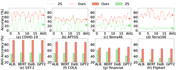
Figure 3: Results on CV (a-d) and NLP (e-h) tasks.

4.3 Analysis and Discussion

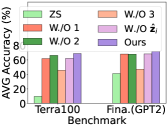
(a) Ablation of each part

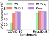
(b) Other observations

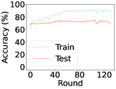
(c) Convergence

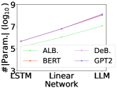
(d) Number of param.

Figure 4: Ablation study, convergence, and communication costs.

Ablation Study. Figure 4(a) and 4(b) give experiments on ablation study and we have following observations. 1) In most situations, each part of our method brings improvements on both CV and NLP. 2) Step 3 is more significant than Step 2. Since Step 3 re-maps outputs, it can offer semantic meanings to foundation models for specific tasks, which is more direct and effective intuitively. Step 2 transforms inputs that still go through foundation models or even random projections, and thereby it is indirect and less effective. However, by combining Step 2 with Step 3, we can achieve further improvements. 3) In some situations, client-specific embeddings do not bring remarkable improvements, which can be induced by two reasons. First, CGE is not stable enough and we cannot ensure ZooPFL finds the best global optimals. Second, to ensure fairness, we offer comparison methods without client-specific embeddings containing larger dimensions and thereby these methods can learn better representations for auto-encoders. 4) Step 1 brings significant improvement for CV while it is less effective for NLP. This can be due to two reasons. We provide better auto-encoders for CV but simple linear layers for NLP. Moreover, the closed pretraining of an auto-encoder without subsequent adjustments to the decoder may not be suitable for NLP. Fortunately, ZooPFL can achieve convincing improvements compared to ZS no matter whether adopting step 1.

Convergence and Communication Cost. We provide convergence analysis and communication cost comparisons in Figure 4(c) and 4(d), respectively. Figure 4(c) shows that both the average training accuracy and testing accuracy are convergent. There exist slight disturbances due to instability of CGE and the process of federated learning. Moreover, we can find that there exists a divergence between training and testing, which means there could be further improvements if more generalization techniques could be adopted which we leave as our future work. From Figure 4(d), we can see exchanging in encoders can reduce a significant amount of transmission cost, especially for LSTM, which means our method can be employed in reality.

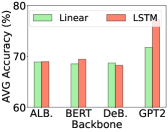
(a) Backbone

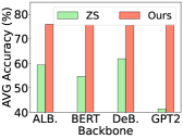
(b) Data splits

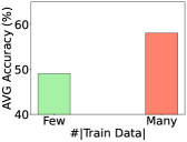
(c) Data size

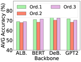
(d) Optimization order

Figure 5: More discussions by varying backbones, data splits, data sizes, and optimization order.

More insightful analysis. 1) Can stronger backbones bring better performance? From Figure 5(a) and 4(d), we can see that auto-encoders comprised of LSTM can bring better performance with fewer communications (especially for GPT2), which means more suitable backbones can lead to better performance. 2) How can data splits influence the performance? Figure 5(b) shows that ZooPFL still achieves better performance when using a different parameter for Dirichlet distribution ($0.1$ vs. $0.2$) for NLP data split. In this more personalized situation, ZS maintains a similar performance while ours performs better. 3) More training data, better results? As shown in Figure 5(c), we choose the APTOS dataset where our method has the worst performance, to evaluate the influence of training data. We find that more training data can bring further improvements, which is completely consistent with our intuition. 4) Can optimization order influence performance? We provide three orders for optimization. Order 1 is what we adopted. Order 2 is to perform step 2 for all rounds and then perform step 3, which means these two steps are split. In order 3, we first optimize the encoder, then client-specific embeddings, and finally semantic re-mapping layers, and these parts are iterative. As shown in Figure 5(d), Order 1 and Order 3 can perform slightly better than Order 2, which demonstrates the necessity of joint optimization.

Parameter sensitivity. Figure 6 provides parameter sensitivity and we obtain following observations. 1) Our method is stable for a wide range of parameters although CGE may lead instability. 2) For most situations, larger learning rates with Adam can bring better performance. 3) ZooPFL can achieve further improvement if we finetune hyperparameters more carefully. For example, we can choose larger learning rates, e.g.$0.5$ or choose more suitable $\rho$ for specific tasks, e.g. $0.05$ for CV.

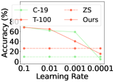
(a) Learning rate (CV)

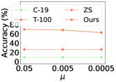
(b) $\rho$ (CV)

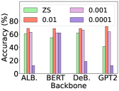
(c) Learning rate (NLP)

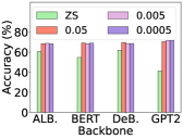
(d) $\rho$ (NLP)

Figure 6: Parameter sensitivity of computer vision and natural language tasks (on finance data).

Sec. 5 Conclusion and Discussion

We proposed ZooPFL which can deal with large black-box models in federated learning. ZooPFL mainly consists of two parts, including input surgery and semantic re-mapping. Moreover, with a client-specific embedding, ZooPFL can be more personalized. We demonstrated its effectiveness on both CV and NLP tasks. ZooPFL achieved remarkable performance without large communication costs and high demands of GPUs.

As the first exploration in black-box federated learning for large foundation models, ZooPFL can be more perfect by pursuing the following avenues. 1) Since the stability and speed of CGE influence the performance of step 2, it can be better to seek more stable and efficient optimization algorithms. 2) Foundation models in ZooPFL can be enhanced by other ways, e.g., auxiliary models, to serve as a complement to foundation models. 3) Experiments with larger foundation models can be performed for evaluation if computational resources are enough in the future.

Appendix A Proofs

The proof is based on the theoretic work of personalized federate learning pioneered in Pillutla et al. (2022). Firstly, we will make some assumptions on our models (parameters) akin to those in Pillutla et al. (2022) with some differences specific to our scenario. One can refer Pillutla et al. (2022) for more details.

Recall that our loss function is defined as follows:

$$F(\mathbf{\hat{u}},\mathbf{v})={{1}\over{n}}\sum_{i=1}^{n}F_{i}(\mathbf{\hat{u}},\mathbf{v}_{i}),$$ (15)

where $F_{i}(\mathbf{\hat{u}},\mathbf{v}_{i})=\mathbb{E}_{\mathbf{x}\sim\mathcal{D}_{i}}f_{i}(\mathbf{\hat{u}},\mathbf{v}_{i},\mathbf{x})$. $\mathbf{\hat{u}}$ denotes the sharing parameters, i.e. parameters of $s_{i}$, while $\mathbf{v}_{i}$ denotes parameters preserved in each client. According to the structure of ZooPFL, $\mathbf{v}_{i}$ is also decomposed into two parts: $\mathbf{v}_{i}=\mathbf{v}_{1,i}\cup\mathbf{v}_{2,i}$ corresponding to parameters of $\hat{\mathbf{z}_{i}}$ and $r_{i}$ respectively, and as pointed out in main sections of our paper, we regroup our parameters as follows: for each device $i$, $\mathbf{u}_{i}:=\mathbf{\hat{u}}\cup\mathbf{v}_{1,i}$, $\mathbf{v}_{i}:=\mathbf{v}_{2,i}$.

Assumption 1.

(Smoothness). For each device $i=1,2,\dots n$, the object $F_{i}$ is smooth, i.e., it is continuously differentiable and,

1. $\mathbf{u}_{i}\rightarrow\nabla_{\mathbf{u}}F_{i}(\mathbf{u}_{i},\mathbf{v}_{i})$ is $L_{\mathbf{u}}$-Lipschitz for all $\mathbf{v}_{i}$ ,

2. $\mathbf{v}_{i}\rightarrow\nabla_{\mathbf{v}}F_{i}(\mathbf{u}_{i},\mathbf{v}_{i})$ is $L_{\mathbf{v}}$-Lipschitz for all $\mathbf{u}_{i}$ ,

3. $\mathbf{v}_{i}\rightarrow\nabla_{\mathbf{u}}F_{i}(\mathbf{u}_{i},\mathbf{v}_{i})$ is $L_{\mathbf{uv}}$-Lipschitz for all $\mathbf{u}_{i}$, and,

4. $\mathbf{u}_{i}\rightarrow\nabla_{\mathbf{v}}F_{i}(\mathbf{u}_{i},\mathbf{v}_{i})$ is $L_{\mathbf{vu}}$-Lipschitz for all $\mathbf{v}_{i}$.

Further, we assume for some $\chi>0$ that

$$max\{L_{\mathbf{uv}},L_{\mathbf{vu}}\}\leq\chi\sqrt{L_{\mathbf{u}}L_{\mathbf{v}}}.$$ (16)

Assumption 2.

(Bounded Gradient). For each device $i=1,2,\dots n$, the object $F_{i}$ has bounded gradient, that is, there exists $M_{\mathbf{u}},M_{\mathbf{v}}>0$ such that

$$|\nabla_{\mathbf{u}}f_{i}(\mathbf{u}_{i},\mathbf{v}_{i},\mathbf{x})|<M_{\mathbf{u}},\quad and\quad|\nabla_{\mathbf{v}}f_{i}(\mathbf{u}_{i},\mathbf{v}_{i},\mathbf{x})|<M_{\mathbf{v}}\quad\forall\mathbf{x}\in\mathcal{D}_{i}.$$ (17)

Assumption 3.

(Bounded Variance). Let $\mathcal{D}_{i}$ denote a probability distribution over the data space $\mathcal{Z}$ on device $i$. There exist functions $G_{i,\mathbf{u}}$ and $G_{i,\mathbf{v}}$ which are unbiased estimates of $\nabla_{\mathbf{u}}F_{i}$ and $\nabla_{\mathbf{v}}F_{i}$ respectively. That is, for all $\mathbf{u}_{i},\mathbf{v}_{i}$:

$$\mathbb{E}_{\mathbf{x}\sim\mathcal{D}_{i}}[G_{i,\mathbf{u}}(\mathbf{u}_{i},\mathbf{v}_{i},\mathbf{x})]=\nabla_{\mathbf{u}}F_{i}(\mathbf{u}_{i},\mathbf{v}_{i}),\quad and\quad\mathbb{E}_{\mathbf{x}\sim\mathcal{D}_{i}}[G_{i,\mathbf{v}}(\mathbf{u}_{i},\mathbf{v}_{i},\mathbf{x})]=\nabla_{\mathbf{v}}F_{i}(\mathbf{u}_{i},\mathbf{v}_{i}).$$ (18)

Furthermore, the variance of these estimators is at most $\sigma_{\mathbf{u}}^{2}$ and $\sigma_{\mathbf{v}}^{2}$ respectively. That is,

$$\mathbb{E}_{\mathbf{x}\sim\mathcal{D}_{i}}||G_{i,\mathbf{u}}(\mathbf{u}_{i},\mathbf{v}_{i},\mathbf{x})-\nabla_{\mathbf{u}}F_{i}(\mathbf{u}_{i},\mathbf{v}_{i})||^{2}\leq\sigma^{2}_{\mathbf{u}},$$ (19)

$$\mathbb{E}_{\mathbf{x}\sim\mathcal{D}_{i}}||G_{i,\mathbf{v}}(\mathbf{u}_{i},\mathbf{v}_{i},\mathbf{x})-\nabla_{\mathbf{v}}F_{i}(\mathbf{u}_{i},\mathbf{v}_{i})||^{2}\leq\sigma^{2}_{\mathbf{v}}.$$ (20)

In this work, we usually take the particular form $G_{i,\mathbf{u}}(\mathbf{u}_{i},\mathbf{v}_{i},\mathbf{x})=\nabla_{\mathbf{u}}f_{i}((\mathbf{u}_{i},\mathbf{v}_{i}),\mathbf{x})$, which is the gradient of the loss on datatpoint $\mathbf{x}\sim\mathcal{D}_{i}$ under the model $(\mathbf{u}_{i},\mathbf{v}_{i})$, and similarly for $G_{i,\mathbf{v}}$.

As our model has a black box LLM, we can’t get the gradient of parameters in this part. So we resort to zero-order optimization partially. In particular, we take differences of function values to estimate unknown gradients in that part. The resulting method is dubbed stochastic difference descent method. More precisely, Let $G$ be a continuous function on $\mathbf{x}$, $\bm{\rho}$ be a fixed vector with the same dimension of $\mathbf{x}$ and its norm $||\bm{\rho}||=\rho$, we denote $\Delta_{\bm{\rho},\mathbf{x}}G({x}):=(G(\mathbf{x}+\bm{\rho})-G(\mathbf{x}))/\rho$ or $(G(\mathbf{x}+\bm{\rho})+G(\mathbf{x}-\bm{\rho})-2G(\mathbf{x}))/(2\rho)$ to be the difference of $G$ at point $\mathbf{x}$ with step $\bm{\rho}$. Then the way we update $\mathbf{x}$ is similar to that in stochastic gradient descent method:

$$\mathbf{x}_{k+1}=\mathbf{x}_{k}-\gamma\Delta_{\bm{\rho},\mathbf{x}}G(\mathbf{x})|_{\mathbf{x}=\mathbf{x}_{k}}.$$ (21)

Let us denote $\tilde{G}_{i,\mathbf{u}}(\mathbf{u}_{i},\mathbf{v}_{i},\mathbf{x}):=\Delta_{\bm{\rho},\mathbf{u}}f_{i}((\mathbf{u}_{i},\mathbf{v}_{i}),\mathbf{x}),\tilde{G}_{i,\mathbf{v}}(\mathbf{u}_{i},\mathbf{v}_{i},\mathbf{x}):=\Delta_{\bm{\rho},\mathbf{v}}f_{i}((\mathbf{u}_{i},\mathbf{v}_{i}),\mathbf{x})$. Unlike Assumption. 3, $\tilde{G}_{i,\mathbf{u}}(\mathbf{u}_{i},\mathbf{v}_{i},\mathbf{x})$(resp.$\tilde{G}_{i,\mathbf{v}}(\mathbf{u}_{i},\mathbf{v}_{i},\mathbf{x})$) is not an unbiased estimation of $\nabla_{\mathbf{u}}F_{i}(\mathbf{u}_{i},\mathbf{v}_{i})$ (resp.$\nabla_{\mathbf{v}}F_{i}(\mathbf{u}_{i},\mathbf{v}_{i})$). However, under Assumption. 1,Assumption. 2 and Assumption. 3, we have the following estimates:

Lemma 1.

(Bounded 1st and 2nd moments).

$$||\mathbb{E}_{\mathbf{x}\sim\mathcal{D}_{i}}\tilde{G}_{i,\mathbf{u}}(\mathbf{u}_{i},\mathbf{v}_{i},\mathbf{x})-\nabla_{\mathbf{u}}F_{i}(\mathbf{u}_{i},\mathbf{v}_{i})||\leq L_{\mathbf{u}}\rho,$$ (22)

$$||\mathbb{E}_{\mathbf{x}\sim\mathcal{D}_{i}}\tilde{G}_{i,\mathbf{v}}(\mathbf{u}_{i},\mathbf{v}_{i},\mathbf{x})-\nabla_{\mathbf{v}}F_{i}(\mathbf{u}_{i},\mathbf{v}_{i})||\leq L_{\mathbf{u}}\rho.$$ (23)

Furthermore,

$$\mathbb{E}_{\mathbf{x}\sim\mathcal{D}_{i}}||\tilde{G}_{i,\mathbf{u}}(\mathbf{u}_{i},\mathbf{v}_{i},\mathbf{x})-\nabla_{\mathbf{u}}F_{i}(\mathbf{u}_{i},\mathbf{v}_{i}))||^{2}\leq 2L_{\mathbf{u}}^{2}\rho^{2}+2\sigma_{\mathbf{u}}^{2},$$ (24)

$$\mathbb{E}_{\mathbf{x}\sim\mathcal{D}_{i}}||\tilde{G}_{i,\mathbf{v}}(\mathbf{u}_{i},\mathbf{v}_{i},\mathbf{x})-\nabla_{\mathbf{v}}F_{i}(\mathbf{u}_{i},\mathbf{v}_{i}))||^{2}\leq 2L_{\mathbf{v}}^{2}\rho^{2}+2\sigma_{\mathbf{v}}^{2}.$$ (25)

Proof.

For each $\mathbf{x}\in\mathcal{D}_{i}$ there exists a $\mathbf{u}^{\prime}_{i}$ between $\mathbf{u}_{i}$ and $\mathbf{u}_{i}+\bm{\rho}$ in each component such that $(\nabla_{\mathbf{u}}f_{i}(\mathbf{u}_{i}+\bm{\rho},\mathbf{v}_{i},\mathbf{x})-\nabla_{\mathbf{u}}f_{i}(\mathbf{u}_{i},\mathbf{v}_{i},\mathbf{x}))/\rho=\nabla_{\mathbf{u}}f_{i}(\mathbf{u}^{\prime}_{i},\mathbf{v}_{i},\mathbf{x})$. Then by the smoothness assumption:

$$||\nabla_{\mathbf{u}}f_{i}(\mathbf{u}^{\prime}_{i},\mathbf{v}_{i},\mathbf{x})-\nabla_{\mathbf{u}}f_{i}(\mathbf{u}_{i},\mathbf{v}_{i},\mathbf{x})||\leq L_{\mathbf{u}}||\mathbf{u}^{\prime}_{i}-\mathbf{u}_{i}||\leq L_{\mathbf{u}}||\bm{\rho}||=L_{\mathbf{u}}\rho.$$ (26)

Thus

$$\tilde{G}_{i,\mathbf{u}}(\mathbf{u}_{i},\mathbf{v}_{i},\mathbf{x})-\nabla_{\mathbf{u}}F_{i}(\mathbf{u}_{i},\mathbf{v}_{i})=$$ (27)

$$\tilde{G}_{i,\mathbf{u}}(\mathbf{u}_{i},\mathbf{v}_{i},\mathbf{x})-\nabla_{\mathbf{u}}f_{i}((\mathbf{u}_{i},\mathbf{v}_{i}),\mathbf{x})+\nabla_{\mathbf{u}}f_{i}((\mathbf{u}_{i},\mathbf{v}_{i}),\mathbf{x})-\nabla_{\mathbf{u}}F_{i}(\mathbf{u}_{i},\mathbf{v}_{i}).$$ (28)

Taking expectation on both sides and applying equation 26 and $\mathbb{E}_{\mathbf{x}\sim\mathcal{D}_{i}}\nabla_{\mathbf{u}}f_{i}((\mathbf{u}_{i},\mathbf{v}_{i}),\mathbf{x})=\nabla_{\mathbf{u}}F_{i}(\mathbf{u}_{i},\mathbf{v}_{i})$, we get

$$\mathbb{E}_{\mathbf{x}\sim\mathcal{D}_{i}}\tilde{G}_{i,\mathbf{u}}(\mathbf{u}_{i},\mathbf{v}_{i},\mathbf{x})-\nabla_{\mathbf{u}}F_{i}(\mathbf{u}_{i},\mathbf{v}_{i})=\mathbb{E}_{\mathbf{x}\sim\mathcal{D}_{i}}\tilde{G}_{i,\mathbf{u}}(\mathbf{u}_{i},\mathbf{v}_{i},\mathbf{x})-\nabla_{\mathbf{u}}f_{i}((\mathbf{u}_{i},\mathbf{v}_{i}),\mathbf{x})$$ (29)

$$\leq\mathbb{E}_{\mathbf{x}\sim\mathcal{D}_{i}}|\tilde{G}_{i,\mathbf{u}}(\mathbf{u}_{i},\mathbf{v}_{i},\mathbf{x})-\nabla_{\mathbf{u}}f_{i}((\mathbf{u}_{i},\mathbf{v}_{i}),\mathbf{x})|\leq L_{\mathbf{u}}\rho.$$ (30)

Taking absolute values on both sides completes the proof of equation 22. The same is true for equation 23.

For equation 24 and equation 25, we note that by Cauchy-Schwartz inequality

$$||\tilde{G}_{i,\mathbf{u}}(\mathbf{u}_{i},\mathbf{v}_{i},\mathbf{x})-\nabla_{\mathbf{u}}F_{i}(\mathbf{u}_{i},\mathbf{v}_{i})||^{2} \leq 2||\tilde{G}_{i,\mathbf{u}}(\mathbf{u}_{i},\mathbf{v}_{i},\mathbf{x})-\nabla_{\mathbf{u}}f_{i}(\mathbf{u}_{i},\mathbf{v}_{i},\mathbf{x})||^{2}$$ (31)

$$+2||\nabla_{\mathbf{u}}f_{i}(\mathbf{u}_{i},\mathbf{v}_{i},\mathbf{x})-\nabla_{\mathbf{u}}F_{i}(\mathbf{u}_{i},\mathbf{v}_{i})||^{2}.$$ (32)

Taking expectation on both sides and using equation 26 and Assumption. 3 complete the proof. The same is true for equation 25.

∎

As our model has the form $F=r\circ J\circ s$ with $s$ corresponding to the encoder, $J$ corresponding to decoder and black-box LLM, and $r$ corresponding to linear remapping, the following corollary is useful.

Corollary 2.

Let $s_{i},J_{i},r_{i}$ be three continuously differentiable functions such that $f_{i}(\mathbf{u}_{i},\mathbf{v}_{i},\mathbf{x})=r_{i}\circ J_{i}\circ s_{i}$, then we have

$$||\mathbb{E}_{\mathbf{x}\sim\mathcal{D}_{i}}\nabla r_{i,\mathbf{u}}\circ\Delta_{\bm{\rho}}J_{i,\mathbf{u}}\circ\nabla_{\mathbf{u}}s_{i,\mathbf{u}}(\mathbf{u}_{i},\mathbf{v}_{i},\mathbf{x})-\nabla_{\mathbf{u}}F_{i}(\mathbf{u}_{i},\mathbf{v}_{i})||\leq M_{\mathbf{u}}^{2}L_{\mathbf{u}}\rho,$$ (33)

$$||\mathbb{E}_{\mathbf{x}\sim\mathcal{D}_{i}}\nabla r_{i,\mathbf{u}}\circ\Delta_{\bm{\rho}}J_{i,\mathbf{u}}\circ\nabla_{\mathbf{v}_{i}}s_{i,\mathbf{u}}(\mathbf{u}_{i},\mathbf{v}_{i},\mathbf{x})-\nabla_{\mathbf{v}}F_{i}(\mathbf{u}_{i},\mathbf{v}_{i})||\leq M_{\mathbf{v}}^{2}L_{\mathbf{v}}\rho.$$ (34)

Furthermore,

$$\mathbb{E}_{\mathbf{x}\sim\mathcal{D}_{i}}||\nabla r_{i,\mathbf{u}}\circ\Delta_{\bm{\rho}}J_{i,\mathbf{u}}\circ\nabla_{\mathbf{u}}s_{i,\mathbf{u}}(\mathbf{u}_{i},\mathbf{v}_{i},\mathbf{x})-\nabla_{\mathbf{u}}F_{i}(\mathbf{u}_{i},\mathbf{v}_{i})||^{2}\leq 2M_{\mathbf{u}}^{4}L_{\mathbf{u}}^{2}\rho^{2}+2\sigma_{\mathbf{u}}^{2},$$ (35)

$$\mathbb{E}_{\mathbf{x}\sim\mathcal{D}_{i}}||\nabla r_{i,\mathbf{u}}\circ\Delta_{\bm{\rho}}J_{i,\mathbf{u}}\circ\nabla_{\mathbf{v}_{i}}s_{i,\mathbf{u}}(\mathbf{u}_{i},\mathbf{v}_{i},\mathbf{x})-\nabla_{\mathbf{v}}F_{i}(\mathbf{u}_{i},\mathbf{v}_{i})||^{2}\leq 2M_{\mathbf{v}}^{4}L_{\mathbf{v}}^{2}\rho^{2}+2\sigma_{\mathbf{v}}^{2}.$$ (36)

Proof.

Using the bounded gradient assumption and following the steps in the proof of Lemma. 1 completes the proof. ∎

Finally, we make a gradient diversity assumption.

Assumption 4.

(Partial Gradient Diversity). There exists $\delta\geq 0$ and $\mu\geq 0$ such that for all $\mathbf{u}$ and $\mathbf{v}$,

$$\frac{1}{n}\sum_{i=1}^{n}||\nabla_{\mathbf{u}}F_{i}(\mathbf{u}_{i},\mathbf{v}_{i})-\nabla_{\mathbf{u}}F(\mathbf{u},\mathbf{v})||^{2}\leq\delta^{2}+\mu^{2}||\nabla_{\mathbf{u}}F(\mathbf{u},\mathbf{v})||^{2}.$$ (37)

Please refer Pillutla et al. (2022) for more background on some of these assumptions.

A.1 Convergence Analysis of ZooPFL

We give the error bounds results of Algorithm 1, thus theoretically establishing the convergence property.

In our case, we rename the parameters so that $\mathbf{u}:=\mathbf{\hat{u}}\cup\mathbf{v}_{1},\mathbf{v}:=\mathbf{v}_{2}$. As per Appendix A.3 in Pillutla et al. (2022), we use the constants

$$\sigma^{2}_{alt,1} =\frac{\delta^{2}}{L_{\mathbf{u}}}\left(1-\frac{m}{n}\right)+\frac{2M_{\mathbf{u}}^{4}L_{\mathbf{u}}^{2}\rho^{2}+2\sigma^{2}_{\mathbf{u}}}{L_{\mathbf{u}}}+\frac{(2M_{\mathbf{v}}^{4}L_{\mathbf{v}}^{2}\rho^{2}+2\sigma_{\mathbf{v}}^{2})(m+\chi^{2}(n-m))}{L_{\mathbf{v}}n},$$ (38)

$$\sigma^{2}_{alt,2} =\frac{2M_{\mathbf{u}}^{4}L_{\mathbf{u}}^{2}\rho^{2}+2\sigma^{2}_{\mathbf{u}}+\delta^{2}}{L_{\mathbf{u}}}(1-\tau_{\mathbf{u}}^{-1})$$ (39)

$$+\frac{(2M_{\mathbf{v}}^{4}L_{\mathbf{v}}^{2}\rho^{2}+2\sigma_{\mathbf{v}}^{2})m}{L_{\mathbf{v}}n}(1-\tau_{\mathbf{u}}^{-1})+\frac{\chi^{2}(2M_{\mathbf{v}}^{4}L_{\mathbf{v}}^{2}\rho^{2}+2\sigma^{2}_{\mathbf{v}})}{L_{\mathbf{v}}}.$$ (40)

and the definitions

$$\Delta_{\mathbf{u}}^{{(t)}}=\frac{1}{n}\sum_{i=1}^{n}||\nabla_{\mathbf{u}}F_{i}\left(\mathbf{u}_{i}^{(t)},\mathbf{v}_{i}^{(t)}\right)||^{2},\quad and,\quad\Delta_{\mathbf{v}}^{(t)}=\frac{1}{n}\sum^{n}_{i=1}||\nabla_{\mathbf{v}}F_{i}\left(\mathbf{u}_{i}^{(t)},\mathbf{v}_{i}^{(t)}\right)||^{2}.$$ (41)

Theorem 1.

Suppose Assumption. 1,Assumption. 2,Assumption. 3 and Assumption. 4 hold and the learning rates in ZooPFL are chosen as $\gamma_{\mathbf{u}}=\eta/(L_{\mathbf{u}}\tau_{\mathbf{u}})$ and $\gamma_{\mathbf{v}}=\eta/(L_{\mathbf{v}}\tau_{\mathbf{v}})$, with

$$\eta\leq\textit{min}\left\{{1\over 24(1+\mu^{2})},\frac{m}{128\chi^{2}(n-m)},\sqrt{m\over\chi^{2}n}\right\}.$$ (42)

Then, right after the training of $T$ epochs, ignoring absolute constants, we have

$$\frac{1}{T}\sum_{t=0}^{T-1}\left(\frac{1}{L_{\mathbf{u}}}\mathbb{E}\left[\Delta_{\mathbf{u}}^{(t)}\right]+\frac{m}{nL_{\mathbf{v}}}\mathbb{E}\left[\Delta_{\mathbf{v}}^{(t)}\right]\right)\leq\frac{\Delta F_{0}}{\eta T}+\eta\sigma^{2}_{alt,1}+\eta^{2}\sigma^{2}_{alt,2}.$$ (43)

Corollary 3.

An optimal learning rate is chosen as follows

$$\eta=\left(\frac{\Delta F_{0}}{T\sigma_{alt,1}^{2}}\right)^{1/2}\bigwedge\left(\frac{\Delta F_{0}^{2}}{T^{2}\sigma_{alt,2}^{2}}\right)^{1/3}\bigwedge\frac{1}{1+\mu^{2}}\bigwedge\frac{m}{\chi^{2}(n-m)}\bigwedge\sqrt{\frac{m}{\chi^{2}n}}.$$ (44)

We have, ignoring absolute constants,

$$\frac{1}{T}\sum_{t=0}^{T-1}\left(\frac{1}{L_{\mathbf{u}}}\mathbb{E}\left[\Delta_{\mathbf{u}}^{(t)}\right]+\frac{m}{nL_{\mathbf{v}}}\mathbb{E}\left[\Delta_{\mathbf{v}}^{(t)}\right]\right)\leq$$ (45)

$$\frac{(\Delta F_{0}\sigma_{alt,1}^{2})^{1/2}}{\sqrt{T}}+\frac{(\Delta F_{0}^{2}\sigma_{alt,2}^{2})^{1/3}}{T^{2/3}}+\frac{\Delta F_{0}}{T}\left(1+\mu^{2}+\chi^{2}(\frac{n}{m}-1)+\sqrt{\chi^{2}\frac{n}{m}}\right).$$ (46)

Proof.

The proof is invoking Lemma 25 in Pillutla et al. (2022) upon establishing Thm. 1 ∎

We will refer the readers to Pillutla et al. (2022) for the proof of convergence of FedAlt algorithm therein. One of our novel differences to Pillutla et al. (2022) is that our black-box model is secure so its gradient is invisible to us, leading us to consider zero-order (gradient free) optimization. Thus we first establish a result analogous to lemma 22 in Pillutla et al. (2022) for zero-order optimization.

Lemma 2.

Consider $f:R^{d}\rightarrow R$ which is $L$-smooth, its norm of gradient is bounded by $M$ and fix a $\mathbf{w}^{{(0)}}\in R^{d}$. Define the sequence $(\mathbf{w}^{(t)})$ of iterates produced by stochastic difference descent with step $\bm{\rho}$ and a fixed learning rate $\gamma$ starting from $\mathbf{w}^{(0)}$:

$$\mathbf{w}^{(t+1)}=\mathbf{w}^{(t)}-\gamma\tilde{g}^{(t)},$$ (47)

where $\tilde{g}$ is an unbiased estimation to $\Delta_{\bm{\rho},\mathbf{w}}f(\mathbf{w}^{(t)})$ (not an unbiased estimation to $\nabla f(\mathbf{w}^{(t)})$) with bounded variance $2M^{4}L^{2}\rho^{2}+2\sigma^{2}$. Fix a number $\tau$ of steps. If $\gamma\leq(\sqrt{2}\tau L)^{-1}$, we have the bound

$$\sum_{t=0}^{\tau-1}||\mathbf{w}^{(t)}-\mathbf{w}^{(0)}||^{2}\leq 8\gamma^{2}\tau^{2}(\tau-1)||\nabla f(\mathbf{w}^{(0)})||^{2}+4\gamma^{2}\tau^{2}(\tau-1)(2M^{4}L^{2}\rho^{2}+2\sigma^{2}).$$ (48)

Proof.

If $\tau=1$, we have nothing to prove. Assume now that $\tau\geq 2$. Let $\mathcal{F}^{(t)}$ be the sigma-algebra generated by $\mathbf{w}^{(t)}$ and denote $\mathbb{E}_{t}[\cdot]=\mathbb{E}[\cdot|\mathcal{F}^{(t)}]$. We will use the inequality

$$\mathbb{E}_{t}||\tilde{g}^{(t)}||^{2}=\mathbb{E}_{t}||\tilde{g}^{(t)}-\nabla f(\mathbf{w}^{(t)})||^{2}+||\nabla f(\mathbf{w}^{(t)})||^{2}\leq 2M^{4}L^{2}\rho^{2}+2\sigma^{2}+||\nabla f(\mathbf{w}^{(t)})||^{2}.$$ (49)

We then successively deduce,

$$\mathbb{E}_{t}||\mathbf{w}^{(t+1)}-\mathbf{w}^{(0)}||^{2} =||\mathbf{w}^{(t)}-\mathbf{w}^{(0)}-\gamma\tilde{g}^{(t)}||^{2}$$ (50)

$$\leq\left(1+\frac{1}{\tau-1}\right)||\mathbf{w}^{(t)}-\mathbf{w}^{(0)}||^{2}+\gamma^{2}\tau\mathbb{E}_{t}||\tilde{g}^{(t)}||^{2}$$ (51)

$$\leq\left(1+\frac{1}{\tau-1}\right)||\mathbf{w}^{(t)}-\mathbf{w}^{(0)}||^{2}+2\gamma^{2}\tau||\nabla f(\mathbf{w}^{(t)}-\nabla f(\mathbf{w}^{(0)})||^{2}$$ (52)

$$+2\gamma^{2}\tau||\nabla f(\mathbf{w}^{(0)})||^{2}+\gamma^{2}\tau(2M^{4}L^{2}\rho^{2}+2\sigma^{2})$$ (53)

$$\leq\left(1+\frac{1}{\tau-1}+2\gamma^{2}\tau L^{2}\right)||\mathbf{w}^{(t)}-\mathbf{w}^{(0)}||^{2}+2\gamma^{2}\tau||\nabla f(\mathbf{w}^{(0)})||^{2}$$ (54)

$$+\gamma^{2}\tau(2M^{4}L^{2}\rho^{2}+2\sigma^{2})$$ (55)

$$\leq\left(1+\frac{2}{\tau-1}\right)||\mathbf{w}^{(t)}-\mathbf{w}^{(0)}||^{2}+2\gamma^{2}\tau||\nabla f(\mathbf{w}^{(0)})||^{2}$$ (56)

$$+\gamma^{2}\tau(2M^{4}L^{2}\rho^{2}+2\sigma^{2}).$$ (57)

Above, we used (a) the inequality $2\alpha\beta\leq\alpha^{2}/\delta^{2}+\delta^{2}\beta^{2}$ for reals $\alpha,\beta,\delta$,(b) equation 49,(c) $L$-smoothness of $f$, and,(d) the condition on the learning rate.

Let $C=2\gamma^{2}\tau||\nabla f(\mathbf{w}^{(0)})||^{2}+\gamma^{2}\tau(2M^{4}L^{2}\rho^{2}+2\sigma^{2})$. Unrolling the inequality and summing up the series for all $t\leq\tau-1$

$$||\mathbf{w}^{(t)}-\mathbf{w}^{(0)}||^{2} \leq C\sum_{j=0}^{t-1}\left(1-\frac{2}{\tau-1}\right)^{j}\leq\frac{C}{2}(\tau-1)\left(1+\frac{2}{\tau-1}\right)^{t}$$ (58)

$$\leq\frac{C}{2}(\tau-1)\left(1+\frac{2}{\tau-1}\right)^{\tau-1}\leq\frac{C}{2}(\tau-1)e^{2},$$ (59)

where we used the bound $(1+1/\alpha)^{\alpha}\leq e$ for all $\alpha>0$. Summing over $t$ and using the numerical bound $e^{2}<8$ completes the proof.

∎

Lemma 3.

Consider the setting of Lemma. 2. If $\gamma\leq(2\tau L)^{-1}$, we have the bound

$$||\mathbf{w}^{(\tau)}-\mathbf{w}^{(0)}||^{2}\leq 16\gamma^{2}\tau^{2}||\nabla f(\mathbf{w}^{(0)})||^{2}+8\gamma^{2}\tau^{2}(2M^{4}L^{2}\rho^{2}+2\sigma^{2}).$$ (60)

Proof.

Proceeding similar to the last proof (expect using $\delta=\tau$) gives us

$$\mathbb{E}_{t}||\mathbf{w}^{(t+1)}-\mathbf{w}^{(0)}||^{2}\leq\left(1+\frac{2}{\tau}\right)||\mathbf{w}^{(t)}-\mathbf{w}^{(0)}||^{2}+4\gamma^{2}\tau||\nabla f(\mathbf{w}^{(0)})||^{2}+2\gamma^{2}\tau(2M^{4}L^{2}\rho^{2}+2\sigma^{2}).$$ (61)

Unrolling and summing up the sequence completes the proof, similar to that of Lemma. 2 ∎

With all the preparations, we now take the proof of Thm. 1.

Proof.

Recall that our parameters are renamed as $\mathbf{u}:=\mathbf{\hat{u}}\cup\mathbf{v}_{1},\mathbf{v}:=\mathbf{v}_{2}$.

The first step is to start with

$$F(\mathbf{u}^{(t+1)},\mathbf{v}^{(t+1)})-F(\mathbf{u}^{{(t)}},\mathbf{v}^{{(t)}}) =F(\mathbf{u}^{{(t)}},\mathbf{v}^{(t+1)})-F(\mathbf{u}^{{(t)}},\mathbf{v}^{{(t)}})$$ (62)

$$+F(\mathbf{u}^{(t+1)},\mathbf{v}^{(t+1)})-F(\mathbf{u}^{{(t)}},\mathbf{v}^{(t+1)}).$$ (63)

The first line is referred to $\mathbf{v}$-step and the second $\mathbf{u}$-step. The smoothness assumption bounds the $\mathbf{u}$-step:

$$F(\mathbf{u}^{(t+1)},\mathbf{v}^{(t+1)})-F(\mathbf{u}^{(t)},\mathbf{v}^{(t+1)})=\frac{1}{n}\sum_{i=1}^{n}F_{i}(\mathbf{u}_{i}^{(t+1)},\mathbf{v}_{i}^{(t+1)})-F_{i}(\mathbf{u}_{i}^{(t)},\mathbf{v}_{i}^{(t)})$$ (64)

$$\leq\frac{1}{n}\sum_{i=1}^{n}\left(\left\langle\nabla_{\mathbf{u}}F_{i}(\mathbf{u}_{i}^{(t)},\mathbf{v}_{i}^{(t+1)}),\mathbf{u}_{i}^{(t+1)}-\mathbf{u}_{i}^{(t)}\right\rangle+\frac{L_{\mathbf{u}}}{2}||\mathbf{u}_{i}^{(t+1)}-\mathbf{u}_{i}^{(t)}||^{2}\right).$$ (65)

As discussed in Pillutla et al. (2022), the most challenging thing is that the two terms in angle bracket $\langle\rangle$ are not independent random variables. Indeed, they both depend on the sampling $S^{(t)}$ of devices. The way to circumvent it is to introduce virtual full participation for $\mathbf{v}$-step update to eliminate this dependence structure and obtain a good estimate of the error it introduces. Briefly speaking, virtual full participation for parameters $\mathbf{v}$ is to assume all devices to update the $\mathbf{v}$ parameters (it is just technically assumed but not done in practice) that is independent of sampling of $S^{(t)}$ devices, breaking the dependence between $\mathbf{u}^{(t+1)}$ and $\mathbf{v}^{(t+1)}$. We ask the readers to read Pillutla et al. (2022) for full details.

We use the notation $\tilde{\mathbf{v}}^{(t+1)}$ to denote the virtual update of $\mathbf{v}$. Then the proceeding inequality goes on as:

$$\left\langle\nabla_{\mathbf{u}}F_{i}(\mathbf{u}_{i}^{(t)},\mathbf{v}_{i}^{(t+1)}),\mathbf{u}_{i}^{(t+1)}-\mathbf{u}_{i}^{(t)}\right\rangle+\frac{L_{\mathbf{u}}}{2}||\mathbf{u}_{i}^{(t+1)}-\mathbf{u}_{i}^{(t)}||^{2}$$ (66)

$$=\left\langle\nabla_{\mathbf{u}}F_{i}(\mathbf{u}_{i}^{(t)},\tilde{\mathbf{v}_{i}}^{(t+1)}),\mathbf{u}_{i}^{(t+1)}-\mathbf{u}_{i}^{(t)}\right\rangle+\frac{L_{\mathbf{u}}}{2}||\mathbf{u}_{i}^{(t+1)}-\mathbf{u}_{i}^{(t)}||^{2}$$ (67)

$$+\left\langle\nabla_{\mathbf{u}}F_{i}(\mathbf{u}_{i}^{(t)},\mathbf{v}_{i}^{(t+1)})-\nabla_{\mathbf{u}}F_{i}(\mathbf{u}_{i}^{(t)},\tilde{\mathbf{v}_{i}}^{(t+1)}),\mathbf{u}_{i}^{(t+1)}-\mathbf{u}_{i}^{(t)}\right\rangle$$ (68)

$$\leq\left\langle\nabla_{\mathbf{u}}F_{i}(\mathbf{u}_{i}^{(t)},\tilde{\mathbf{v}_{i}}^{(t+1)}),\mathbf{u}_{i}^{(t+1)}-\mathbf{u}_{i}^{(t)}\right\rangle+L_{\mathbf{u}}||\mathbf{u}_{i}^{(t+1)}-\mathbf{u}_{i}^{(t)}||^{2}$$ (69)

$$+\frac{1}{2L_{\mathbf{u}}}||\nabla_{\mathbf{u}}F_{i}(\mathbf{u}_{i}^{(t)},\mathbf{v}_{i}^{(t+1)})-\nabla_{\mathbf{u}}F_{i}(\mathbf{u}_{i}^{(t)},\tilde{\mathbf{v}_{i}}^{(t+1)})||^{2}$$ (70)

$$\leq\left\langle\nabla_{\mathbf{u}}F_{i}(\mathbf{u}_{i}^{(t)},\tilde{\mathbf{v}_{i}}^{(t+1)}),\mathbf{u}_{i}^{(t+1)}-\mathbf{u}_{i}^{(t)}\right\rangle+L_{\mathbf{u}}||\mathbf{u}_{i}^{(t+1)}-\mathbf{u}_{i}^{(t)}||^{2}$$ (71)

$$+\frac{\chi^{2}L_{\mathbf{v}}}{2}||\tilde{\mathbf{v}}^{(t+1)}-\mathbf{v}_{i}^{(t+1)}||^{2}.$$ (72)

The last two inequalities follow from Young’s inequality and Lipschitzness of $\mathbf{v}_{i}\hookrightarrow\nabla_{\mathbf{u}}F_{i}(\mathbf{u}_{i},\mathbf{v}_{i})$ respectively.

The usage of virtual update is to ensure that $\tilde{\mathbf{v}}^{(t+1)}$ is independent of $S^{(t)}$. This allows us to take an expectation w.r.t the sampling $S^{(t)}$ of the devices.

Recall that under the new parameters $\mathbf{u}$ and $\mathbf{v}$, the only difference to the setting of FedAlt in Pillutla et al. (2022) is that we need zero-order optimization to update $\mathbf{u}$ parameter instead of first-order gradient method. Thus, we can use the calculations in Pillutla et al. (2022) with $F$ replaced by $F_{i}$ and then add them together from 1 to $n$ to similarly arrive at the following expression:

$$\mathbb{E}_{t}\left[F(\mathbf{u}^{(t+1)},\mathbf{v}^{(t+1)})-F(\mathbf{u}^{(t)},\mathbf{v}^{(t+1)})\right]$$ (73)

$$\leq-\frac{\gamma_{\mathbf{u}}\tau_{\mathbf{u}}}{4}\mathbb{E}_{t}[\tilde{\Delta}_{\mathbf{u}}^{(t)}]+\frac{2\gamma_{\mathbf{u}}L_{\mathbf{u}}^{2}}{n}\sum_{i=1}^{n}\sum_{k=0}^{\tau_{\mathbf{u}}-1}\mathbb{E}_{t}||\tilde{\mathbf{u}}_{i,k}^{(t)}-\mathbf{u}^{(t)}||^{2}$$ (74)

$$+4\gamma_{\mathbf{v}}^{2}\tau_{\mathbf{v}}^{2}L_{\mathbf{v}}(2M_{\mathbf{v}}^{4}L_{\mathbf{v}}^{2}\rho^{2}+2\sigma_{\mathbf{v}}^{2})\chi^{2}(1-m/n)$$ (75)

$$+\frac{L_{\mathbf{u}}\gamma_{\mathbf{u}}^{2}\tau_{\mathbf{u}}^{2}}{m}(2M_{\mathbf{u}}^{4}L_{\mathbf{u}}^{2}\rho^{2}+2\sigma_{\mathbf{u}}^{2}+3\delta^{2}(1-\frac{m}{n}))+8\gamma_{\mathbf{v}}^{2}\tau_{\mathbf{v}}^{2}L_{\mathbf{v}}\chi^{2}(1-m/n)\Delta_{\mathbf{v}}^{(t)},$$ (76)

note here $\tilde{\mathbf{u}}_{i,k}^{(t)}$ is $\mathbf{u}$-parameter updates via stochastic difference descent method rather than stochastic gradient descent method. We bound this term with Lemma. 2, invoking the assumption on gradient diversity. And then plugging the resulting estimate back in, we get

$$\mathbb{E}_{t}\left[F(\mathbf{u}^{(t+1)},\mathbf{v}^{(t+1)})-F(\mathbf{u}^{(t)},\mathbf{v}^{(t+1)})\right]$$ (77)

$$\leq-\frac{\gamma_{\mathbf{u}}\tau_{\mathbf{u}}}{8}\mathbb{E}_{t}[\tilde{\Delta}_{\mathbf{u}}^{(t)}]+\frac{L_{\mathbf{u}}\gamma_{\mathbf{u}}^{2}\tau_{\mathbf{u}}^{2}}{m}(2M_{\mathbf{u}}^{4}L_{\mathbf{u}}^{2}\rho^{2}+2\sigma_{\mathbf{u}}^{2}+2\delta^{2}(1-m/n))$$ (78)

$$+4\gamma_{\mathbf{v}}^{2}\tau_{\mathbf{v}}^{2}L_{\mathbf{v}}(2M_{\mathbf{v}}^{4}L_{\mathbf{v}}^{2}\rho^{2}+2\sigma_{\mathbf{v}}^{2})\chi^{2}(1-m/n)$$ (79)

$$+8\gamma_{\mathbf{v}}^{2}\tau_{\mathbf{v}}^{2}L_{\mathbf{v}}\chi^{2}(1-m/n)\Delta_{\mathbf{v}}^{(t)}+8\gamma_{\mathbf{v}}^{2}L_{\mathbf{u}}^{3}\tau_{\mathbf{u}}^{2}(\tau_{\mathbf{u}}-1)(2M_{\mathbf{u}}^{4}L_{\mathbf{u}}^{2}\rho^{2}+2\sigma_{\mathbf{u}}^{2}+2\delta_{\mathbf{u}}^{2}).$$ (80)

The bound on $\mathbf{v}$-step has exactly the same form as presented in Pillutla et al. (2022) since when conditioned on $\mathbf{u}^{(t)},\mathbf{v}^{(t)}$ all functions used in updating $\mathbf{v}$ is continuously differentiable. Plugging this bound on $\mathbf{v}$-step into equation 62, we get

$$\mathbb{E}_{t}\left[F(\mathbf{u}^{(t+1)},\mathbf{v}^{(t+1)}-F(\mathbf{u}^{(t)},\mathbf{v}^{(t)}\right]$$ (81)

$$\leq-\frac{\gamma_{\mathbf{u}}\tau_{\mathbf{u}}}{8}\mathbb{E}_{t}[\tilde{\Delta}_{\mathbf{u}}^{(t)}]-\frac{\gamma_{\mathbf{v}}\tau_{\mathbf{v}}m}{16n}\mathbb{E}_{t}[\Delta_{\mathbf{v}}^{(t)}]+4\gamma_{\mathbf{v}}^{2}L_{\mathbf{v}}\tau_{\mathbf{v}}^{2}(2M_{\mathbf{v}}^{4}L_{\mathbf{v}}^{2}\rho^{2}+2\sigma_{\mathbf{v}}^{2})\left(\frac{m}{n}+\chi^{2}(1-m/n)\right)$$ (82)

$$+\frac{\gamma_{\mathbf{u}}^{2}L_{\mathbf{u}}\tau_{\mathbf{u}}^{2}}{m}(2M_{\mathbf{u}}^{4}L_{\mathbf{u}}^{2}\rho^{2}+2\sigma_{\mathbf{u}}^{2}+2\delta^{2}(1-m/n))+8\gamma_{\mathbf{u}}^{3}L_{\mathbf{u}}^{2}\tau_{\mathbf{u}}^{2}(\tau_{\mathbf{u}}-1)(2M_{\mathbf{u}}^{4}L_{\mathbf{u}}^{2}\rho^{2}+2\sigma_{\mathbf{u}}^{2}+2\delta^{2})$$ (83)

$$+\frac{4\gamma_{\mathbf{v}}^{3}L_{\mathbf{v}}^{2}\tau_{\mathbf{v}}^{2}(\tau_{\mathbf{v}}-1)(2M_{\mathbf{v}}^{4}L_{\mathbf{v}}^{2}\rho^{2}+2\sigma_{\mathbf{v}}^{2})m}{n}.$$ (84)

Taking an unconditional expectation, summing it over $t=0$ to $T-1$ and rearranging this gives

$$\frac{1}{T} =\sum_{t=0}^{T-1}\left(\frac{\gamma_{\mathbf{u}}\tau_{\mathbf{u}}}{8}\mathbb{E}[\tilde{\Delta}_{\mathbf{u}}^{(t)}]+\frac{\gamma_{\mathbf{v}}\tau_{\mathbf{v}}m}{16}\mathbb{E}[\Delta_{\mathbf{v}}^{(t)}]\right)$$ (85)

$$\leq\frac{\Delta F_{0}}{T}+4\gamma^{2}_{\mathbf{v}}L_{\mathbf{v}}\tau_{\mathbf{v}}^{2}(2M_{\mathbf{v}}^{4}L_{\mathbf{v}}^{2}\rho^{2}+2\sigma_{\mathbf{v}}^{2})\left(\frac{m}{n}+\chi^{2}(1-m/n)\right)$$ (86)

$$+\frac{\gamma_{\mathbf{u}}^{2}L_{\mathbf{u}}\tau_{\mathbf{u}}^{2}}{m}(2M_{\mathbf{u}}^{4}L_{\mathbf{u}}^{2}\rho^{2}+2\sigma_{\mathbf{u}}^{2}+2\delta^{2}(1-m/n))$$ (87)

$$+8\gamma_{\mathbf{u}}^{3}L_{\mathbf{u}}^{2}\tau_{\mathbf{u}}^{2}(\tau_{\mathbf{u}}-1)(2M_{\mathbf{u}}^{4}L_{\mathbf{u}}^{2}\rho^{2}+2\sigma_{\mathbf{u}}^{2}+2\delta^{2})+\frac{4\gamma_{\mathbf{v}}^{3}L_{\mathbf{v}}^{2}\tau_{\mathbf{v}}^{2}(\tau_{\mathbf{v}}-1)(2M_{\mathbf{v}}^{4}L_{\mathbf{v}}^{2}\rho^{2}+2\sigma_{\mathbf{v}}^{2})m}{n}.$$ (88)

This is a bound in terms of the virtual updates $\tilde{\mathbf{v}}^{(t+1)}$. Similarly to the manipulations in Pillutla et al. (2022) we can relate $\tilde{\Delta}_{\mathbf{u}}^{(t)}$ with $\Delta_{\mathbf{u}}^{(t)}$. , and finally we get:

$$\frac{1}{T}\sum_{t=0}^{T-1}\left(\frac{\gamma_{\mathbf{u}}\tau_{\mathbf{u}}}{16}\mathbb{E}[\Delta_{\mathbf{u}}^{(t)}]+\frac{\gamma_{\mathbf{v}}\tau_{\mathbf{v}}m}{32n}\mathbb{E}[\Delta_{\mathbf{v}}^{(t)}]\right)$$ (89)

$$\leq\frac{1}{T}\sum_{t=0}^{T-1}\left(\frac{\gamma_{\mathbf{u}}\tau_{\mathbf{u}}}{9}\mathbb{E}[\tilde{\Delta}_{\mathbf{u}}^{(t)}]+\frac{\gamma_{\mathbf{v}}\tau_{\mathbf{v}}m}{16n}\mathbb{E}[\Delta_{\mathbf{v}}^{(t)}]\right)+\gamma_{\mathbf{u}}\tau_{\mathbf{u}}\gamma_{\mathbf{v}}^{2}\tau_{\mathbf{v}}^{2}(2M_{\mathbf{u}}^{4}L_{\mathbf{u}}^{2}\rho^{2}+2\sigma_{\mathbf{u}}^{2})\chi^{2}L_{\mathbf{u}}L_{\mathbf{v}}$$ (90)

$$\leq\frac{\Delta F_{0}}{T}+4\gamma_{\mathbf{v}}^{2}L_{\mathbf{v}}\tau_{\mathbf{v}}^{2}(2M_{\mathbf{v}}^{4}L_{\mathbf{v}}^{2}\rho^{2}+2\sigma_{\mathbf{v}}^{2})\left(\frac{m}{n}+\chi^{2}(1-m/n)\right)$$ (91)

$$+\frac{\gamma_{\mathbf{u}}^{2}L_{\mathbf{u}}\tau_{\mathbf{u}}^{2}}{m}(2M_{\mathbf{u}}^{4}L_{\mathbf{u}}^{2}\rho^{2}+2\sigma_{\mathbf{u}}^{2}+2\delta^{2}(1-m/n))$$ (92)

$$+8\gamma_{\mathbf{u}}^{3}L_{\mathbf{u}}^{2}\tau_{\mathbf{u}}^{2}(\tau_{\mathbf{u}}-1)(2M_{\mathbf{u}}^{4}L_{\mathbf{u}}^{2}\rho^{2}+2\sigma_{\mathbf{u}}^{2}+2\delta^{2})+\frac{4\gamma_{\mathbf{v}}^{3}L_{\mathbf{v}}^{2}\tau_{\mathbf{v}}^{2}(\tau_{\mathbf{v}}-1)(2M_{\mathbf{v}}^{4}L_{\mathbf{v}}^{2}\rho^{2}+2\sigma_{\mathbf{v}}^{2})m}{n}$$ (93)

$$+\gamma_{\mathbf{v}}\tau_{\mathbf{u}}\gamma_{\mathbf{v}}^{2}\tau_{\mathbf{v}}^{2}(2M_{\mathbf{v}}^{4}L_{\mathbf{v}}^{2}\rho^{2}+2\sigma_{\mathbf{v}}^{2})\chi^{2}L_{\mathbf{u}}L_{\mathbf{v}}.$$ (94)

Plugging in $\gamma_{\mathbf{u}}=\eta/(L_{\mathbf{u}}\tau_{\mathbf{u}})$ and $\gamma_{\mathbf{v}}=\eta/(L_{\mathbf{v}}\tau_{\mathbf{v}})$ completes the proof.

∎

Appendix B More Discussion on Related Work

Federated learning makes it possible to perform distributed multi-party computing without comprising privacy (Zhang et al., 2021; Voigt & Von dem Bussche, 2017; McMahan et al., 2017; Yang et al., 2019; Wan et al., 2023; Qi et al., 2023). FedAVG is the baseline algorithm for FL by exchanging parameters instead of raw data, which has been used in many applications (Li et al., 2020a; Banabilah et al., 2022; Rodríguez-Barroso et al., 2023). When FedAVG meets non-iid data, it can suffer from low convergence speed and terrible personalization performance (Sattler et al., 2019). FedProx (Li et al., 2020b) allowed differences among clients and the server while FedBN (Li et al., 2021) preserved local batch normalization layers in each client. Setayesh et al. (2023) proposed PerFedMask, a generalization of FedBABU (Oh et al., 2022), that considers the computational capability of different devices. Xu et al. (2023b) conducted explicit local-global feature alignment by leveraging global semantic knowledge, quantified the benefit of classifier combination for each client, and derived an optimization problem for estimating optimal weights. Some other work considered utilizing knowledge distillation for personalization (Chen et al., 2023c) while some work attempted to achieve robust personalization during testing (Jiang & Lin, 2023). Besides personalization, there also exists research focusing on generalization (Chen & Chao, 2022; Gupta et al., 2022; Qu et al., 2022). Our method can deal with situations where distribution shifts exist.

Since deep learning has entered the era of large foundation models (Bommasani et al., 2021; Xing et al., 2023; Zhuang et al., 2023), some novel issues, e.g. computation costs and communication costs, are coming into being, leading operations on the whole network impossible (Chen et al., 2022; 2023a; Ding et al., 2023). FedPrompt (Zhao et al., 2023) studied prompt tuning in a model split aggregation way using FL while FedCLIP (Lu et al., 2023) designed an attention-based adapter for CLIP (Radford et al., 2021). PromptFL (Guo et al., 2023) utilized the federated prompt training instead of the whole model training in a distributed way while pFedPG (Yang et al., 2023a) deployed a personalized prompt generator at the server to produce client-specific visual prompts. FwdLLM (Xu et al., 2023b) combined BP-free training with parameter-efficient training methods and systematically and adaptively allocated computational loads across devices. These methods all require access to the internals of large models but we view foundation models as black-box in this paper.

Besides data privacy, model privacy also raised attention recently (Mo et al., 2020). Model suppliers are usually more willing to only provide predictions for given inputs or just provide a product that can only generate predictions (Van Dis et al., 2023). In this paper, we view these protected foundation models as black-box models (Guidotti et al., 2018; Ljung, 2001). Little work paid attention to finetuning or optimizing in this field, but most related work focused on attacks (Yang et al., 2023b; c). One related work is FedZO (Fang et al., 2022) which utilized zero-order optimization (Ghadimi & Lan, 2013), but it did not consider utilizing large foundation models. Some other work also made use of zero-order optimization for federated learning (Li & Chen, 2021; Zelikman et al., 2023; Feng et al., 2023), but none of them utilized large black-box foundation models.

Model reprogramming (MR) (Tsai et al., 2020; Xu et al., 2023c; Chen, 2022) provides a similar solution to ZooPFL. It trains the inserted input transformation and output mapping layers while keeping the source pretrained model inact to enable resource-efficient cross-domain machine learning. The main purpose of model reprogramming is to transfer knowledge to targets and it can be viewed as a sub-field of transfer learning. Recently, Arif et al. (2023) proposed the first framework, Reprogrammable-FL, adapting MR to the setting of differentially private federated learning. Reprogrammable-FL learned an input transformation for samples and added learned perturbations to the original samples. It preserved local input transformations and shared output transformation layers, which are totally in contrast to ours. Moreover, ZooPFL is proposed for black-box foundation models and can provide an ideal personalization capability.

Appendix C Methodology

C.1 Algorithm Flow

Algorithm 1 describes the concrete process of our proposed ZooPFL.

Algorithm 1 ZooPFL

Input: $n$ clients’ datasets $\{\mathcal{D}_{i}\}_{i=1}^{n}$
Output: Input surgery, $\{s_{i}\}_{i=1}^{n}$, semantic re-mapping, $\{r_{i}\}_{i=1}^{n}$, client-specific embeddings, $\{\hat{\mathbf{z}_{i}}\}_{i=1}^{n}$

1:for $t=1$ to $T$ do $\triangleright$ Step 1

2:     for $i=1$ to $n$ do

3:         Pretrain Client i according to $\ell_{MSE}=\mathbb{E}_{(\mathbf{x},y)\sim\mathbb{P}(\mathcal{D}_{i})}\left\|o_{i}([q_{i}(\mathbf{x}),\hat{\mathbf{z}_{i}}])-\mathbf{x}\right\|_{2}^{2}$      

4:     Upload $\{w(s_{i})\}_{i=1}^{n}$ to the server

5:     Aggregate weights, $w(s)=\frac{1}{n}\sum_{i=1}^{n}w(s_{i})$

6:     Distribute client weight $w(s)$ to each client

7:for $t=1$ to $T$ do

8:     for $i=1$ to $n$ do $\triangleright$ Step 2

9:         for $k=1$ to $d_{1}+d_{2}$ do $\triangleright$ Compute Gradients via CGE

10:              $\tilde{\mathbf{z}_{1}}=\tilde{\mathbf{z}}+\rho\mathbf{e}_{j},\ell_{\mathbf{x},1}=\ell_{cls}(r_{i}(g(o_{i}(\tilde{\mathbf{z}_{1}},y))))$

11:              $\tilde{\mathbf{z}_{2}}=\tilde{\mathbf{z}}-\rho\mathbf{e}_{j},\ell_{\mathbf{x},2}=\ell_{cls}(r_{i}(g(o_{i}(\tilde{\mathbf{z}_{2}},y))))$

12:              Compute differences on embeddings, $\nabla_{\tilde{\mathbf{z}}}\mathcal{G}(\tilde{\mathbf{z}})\approx\sum_{i=1}^{d_{1}+d_{2}}\frac{\ell_{\mathbf{x},2}-\ell_{\mathbf{x},1}}{2\times\rho}\mathbf{e}_{j}$

13:              Compute gradients, $\nabla_{q_{i}}\ell_{1}=\frac{d\tilde{\mathbf{z}}}{dq_{i}}\frac{d\mathcal{G}}{d\tilde{\mathbf{z}}}\approx\frac{d\mathbf{z}}{dq_{i}}\nabla_{\tilde{\mathbf{z}}}\mathcal{G}(\tilde{\mathbf{z}})_{1}\approx\frac{d\nabla_{\tilde{\mathbf{z}}}\mathcal{G}(\tilde{\mathbf{z}})_{1}\mathbf{z}}{dq_{i}}$

14:              Update parameters, $w(q_{i}^{new})=w(q_{i})-\gamma_{1}\times\nabla_{q_{i}}\ell_{1}$               

15:     Upload $\{w(q_{i}^{new})\}_{i=1}^{n}$ to the server

16:     Aggregate weights, $w(q)=\frac{1}{n}\sum_{i=1}^{n}w(q_{i}^{new})$

17:     Distribute $q$ to clients

18:     for $i=1$ to $n$ do $\triangleright$ Step 3

19:         Train semantic re-mapping according to $\ell_{2}=\mathbb{E}_{(\mathbf{x},y)\sim\mathbb{P}(\mathcal{D}_{i})}\ell_{cls}(r_{i}(\mathcal{F}(\mathbf{x})),y)$      

Appendix D Experiments

D.1 Description of the Datasets

Computer vision datasets.

COVID-19 (Sait et al., 2020). It is a public posterior-anterior chest radiography images dataset with four classes, including 1,281 COVID-19 X-Rays, 3,270 Normal X-Rays, 1,656 viral-pneumonia X-Rays, and 3,001 bacterial-pneumonia X-Rays. We split data into 20 clients via the Dirichlet distribution following (Yurochkin et al., 2019) and each client has different distributions on the label space. In each client, only $10\%$ of data are utilized for training and the rest data are split evenly into two parts for validation and testing respectively.

APTOS (Karthik, 2019). It is an image dataset that judges the severity of diabetic retinopathy on a scale of 0 to 4. The original dataset contains 3,662 training images and 1,928 testing images but it suffers from heavily unbalanced. We only utilize the training part in our setting and we randomly choose 400 samples for classes 0 and 2. Our processed dataset contains 1658 samples. We split data into 20 clients and $20\%$ of data serve for training similar to COVID-19.

Terra Incognita (Beery et al., 2018). It is a common dataset that contains photographs of wild animals taken by camera traps at locations L100, L38, L43, and L46. It totally contains 24,788 samples with 10 classes. We randomly choose two locations, i.e. L46 and L100, to construct two benchmarks, i.e. Terra46 and Terra100. For these two benchmarks, we split data into 20 clients and $20\%$ of data serve for training similar to COVID-19.

Natural language processing datasets.

SST-2 (Wang et al., 2019; Socher et al., 2013). The Stanford Sentiment Treebank contains sentences from movie reviews and the labels come from human annotations of their sentiment. It contains about 67k training samples with two classes. We choose sentences with the number of words ranging from 20 to 50 and obtain 9763 samples. We split data into 20 clients and $20\%$ of data serve for training similar to COVID-19.

COLA (Wang et al., 2019; Warstadt et al., 2019). The Corpus of Linguistic Acceptability contains English acceptability judgments drawn from books and journal articles on linguistic theory and it judges a sequence of words whether it is a grammatical English sentence. It contains 8.5k training samples with two classes. We choose sentences with the number of words less than 30 and obtain 5700 samples in total. For the class with more samples, we randomly choose parts to ensure balance. We split data into 20 clients and $20\%$ of data serve for training similar to COVID-19.

Financial-phrasebank (Malo et al., 2014). It consists of sentences from financial news categorized by sentiment. It contains 4840 samples with three classes, including positive, neutral, and negative. We choose sentences with the number of words less than 60 and obtain 3379 samples in total. We split data into 10 clients and $20\%$ of data serve for training similar to COVID-19.

Flipkart (Vaghani & Thummar, 2023). This dataset contains information on product name, product price, rate, reviews, summary and sentiment. It has 205,053 samples with multiple labels. We choose sentiment analysis as our task and there can be three classes, including positive, neutral, and negative. We choose reviews with lengths more than 30 and we randomly choose parts of classes with more samples for balance. The processed dataset contains 3048 samples for each class. We split data into 20 clients and $20\%$ of data serve for training similar to COVID-19.

D.2 Data Distributions

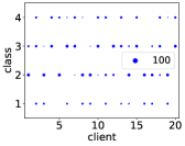
(a) COVID-19 (Train)

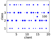
(b) COVID-19 (Test)

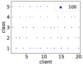
(c) APTOS (Train)

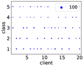
(d) APTOS (Test)

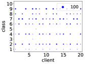
(e) Terra46 (Train)

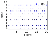
(f) Terra46 (Test)

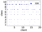
(g) Terra100 (Train)

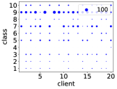
(h) Terra100 (Test)

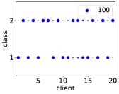
(i) SST-2 (Train)

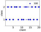
(j) SST-2 (Test)

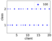
(k) COLA (Train)

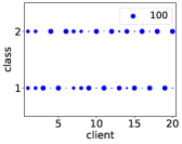
(l) COLA (Test)

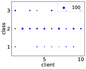
(m) Financial. (Train)

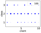
(n) Financial. (Test)

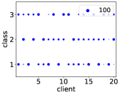
(o) Flipkart (Train)

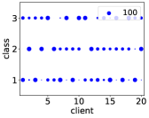
(p) Flipkart (Test)

Figure 7: Data distributions. The size of dots represents the number of samples.

Figure 7 shows the complete data distributions on the rest benchmarks.

D.3 Model Structures

Table 3: The structures of auto-encoders.

CV			NLP(Linear)
Layer(type)	Output Shape	#—Param—	Layer(type)	Output Shape	#—Param—
Conv2d-1	[-1,32,224,224]	896	Linear-1	[-1,128]	6,291,584
ReLU-2	[-1,32,224,224]	0	BatchNorm1d-2	[-1,128]	256
BatchNorm2d-3	[-1,32,224,224]	64	ReLU-3	[-1,128]	0
MaxPool2d-4	[-1,32,112,112]	0	Linear-4	[-1,256]	33,024
Conv2d-5	[-1,64,112,112]	18,496	BatchNorm1d-5	[-1,256]	512
ReLU-6	[-1,64,112,112]	0	ReLU-6	[-1,256]	0
BatchNorm2d-7	[-1,64,112,112]	128	Linear-7	[-1,96]	24,672
MaxPool2d-8	[-1,64,56,56]	0	BatchNorm1d-8	[-1,96]	192
Conv2d-9	[-1,128,56,56]	73,856	ReLU-9	[-1,96]	0
ReLU-10	[-1,128,56,56]	0	Linear-10	[-1,256]	33,024
BatchNorm2d-11	[-1,128,56,56]	256	BatchNorm1d-11	[-1,256]	512
MaxPool2d-12	[-1,128,28,28]	0	ReLU-12	[-1,256]	0
Conv2d-13	[-1,32,28,28]	36,896	Linear-13	[-1,128]	32,896
ReLU-14	[-1,32,28,28]	0	BatchNorm1d-14	[-1,128]	256
BatchNorm2d-15	[-1,32,28,28]	64	ReLU-15	[-1,128]	0
MaxPool2d-16	[-1,32,14,14]	0	Linear-16	[-1,49152]	6,340,608
Conv2d-17	[-1,8,14,14]	2,312	Tanh-17	[-1,49152]	0
ReLU-18	[-1,8,14,14]	0	NLP(LSTM)
BatchNorm2d-19	[-1,8,14,14]	16	LSTM-1	[-1,64,128]	459,776
MaxPool2d-20	[-1,8,7,7]	0	Linear-2	[-1,96]	12,384
Linear-21	[-1,294]	115,542	LSTM-3	[-1,64,128]	132,096
ReLU-22	[-1,294]	0	Linear-4	[-1,64,768]	99,072
BatchNorm1d-23	[-1,294]	588	Tanh-5	[-1,64,768]	0
ConvTranspose2d-24	[-1,32,14,14]	2,336
ReLU-25	[-1,32,14,14]	0
BatchNorm2d-26	[-1,32,14,14]	64
ConvTranspose2d-27	[-1,128,28,28]	36,992
ReLU-28	[-1,128,28,28]	0
BatchNorm2d-29	[-1,128,28,28]	256
ConvTranspose2d-30	[-1,64,56,56]	73,792
ReLU-31	[-1,64,56,56]	0
BatchNorm2d-32	[-1,64,56,56]	128
ConvTranspose2d-33	[-1,32,112,112]	18,464
ReLU-34	[-1,32,112,112]	0
BatchNorm2d-35	[-1,32,112,112]	64
ConvTranspose2d-36	[-1,16,224,224]	4,624
ReLU-37	[-1,16,224,224]	0
BatchNorm2d-38	[-1,16,224,224]	32
Conv2d-39	[-1,3,224,224]	51

Table 3 shows details on auto-encoders. Please note that the encoder accounts for approximately half of the parameter count.

D.4 Additional Results

Table 4: Results on four computer vision benchmarks. Bold means the best.

DataSet	Method	1	2	3	4	5	6	7	8	9	10	11	12	13	14	15	16	17	18	19	20	AVG
COVID-19	Zs	18.36	33.66	1.94	48.06	3.38	47.32	53.17	0.00	3.40	51.71	3.90	43.69	40.78	13.17	54.37	0.00	11.65	36.59	0.97	58.05	26.21
	Ours	76.81	42.44	82.04	59.22	82.61	70.24	62.44	79.90	82.04	55.12	58.54	80.58	37.86	71.22	64.08	82.52	72.33	49.27	87.38	66.83	68.17
APTOS	Zs	0.00	53.12	0.00	41.94	0.00	45.16	25.00	32.26	48.39	0.00	29.03	12.50	65.62	0.00	51.61	0.00	40.62	0.00	0.00	38.71	24.20
	Ours	43.33	59.38	54.84	54.84	50.00	41.94	56.25	38.71	51.61	48.39	41.94	53.12	65.62	32.26	48.39	53.12	50.00	36.67	48.39	51.61	49.02
Terra46	Zs	21.93	21.55	25.22	12.39	34.48	6.09	13.04	25.44	33.33	18.42	46.09	6.96	35.96	16.38	41.74	5.31	25.00	7.96	21.74	21.74	22.04
	Ours	48.25	62.07	56.52	70.80	43.97	51.30	45.22	28.95	47.37	62.28	41.74	59.13	34.21	60.34	60.00	59.29	35.34	67.26	50.43	76.52	53.05
Terra100	Zs	14.13	9.89	7.69	9.57	5.56	6.38	9.78	6.45	6.52	16.48	4.40	11.70	11.83	7.78	12.90	7.69	11.96	7.61	9.78	12.22	9.52
	Ours	63.04	73.63	56.04	75.53	65.56	100.00	59.78	96.77	90.22	57.14	51.65	64.89	48.39	80.00	86.02	49.45	52.17	68.48	78.26	60.00	68.85

Table 5: Average results on NLP. Bold means the best.

Benchmark	Method	ALBERT	BERT	DeBERTa	GPT2	AVG
SST-2	ZS	47.84	52.16	52.14	52.14	51.07
	Ours	94.70	94.72	94.70	94.70	94.71
COLA	ZS	50.22	50.22	49.87	48.82	49.78
	Ours	89.34	88.73	88.16	88.46	88.67
Financial	ZS	60.76	54.82	62.11	41.26	54.74
	Ours	68.91	68.54	68.69	71.79	69.48
Flipkart	ZS	32.26	29.43	33.27	34.16	32.28
	Ours	64.85	64.50	66.32	65.50	65.29

Table 6: Results on Financial-phrasebank. Bold means the best.

Backbones	Client	1	2	3	4	5	6	7	8	9	10	AVG
ALBERT	ZS	31.85	91.18	64.71	58.21	78.36	42.96	85.82	38.24	67.41	48.89	60.76
	Ours	52.59	99.26	62.50	58.96	87.31	52.59	94.78	50.00	77.78	53.33	68.91
BERT	ZS	42.22	70.59	58.82	49.25	57.46	47.41	67.16	43.38	58.52	53.33	54.82
	Ours	52.59	99.26	62.50	58.96	87.31	50.37	94.78	44.12	77.78	57.78	68.54
DeBERTa	ZS	25.93	99.26	62.50	58.96	87.31	36.30	94.78	31.62	77.78	46.67	62.11
	Ours	52.59	99.26	66.18	58.96	87.31	42.96	94.78	46.32	77.78	60.74	68.69
GPT2	ZS	41.48	41.18	49.26	37.31	43.28	37.04	48.51	33.82	42.96	37.78	41.26
	Ours	52.59	99.26	75.00	61.94	87.31	52.59	91.04	50.74	81.48	65.93	71.79

Table 4, Table 5, and Table 6 show more detailed results on computer vision and natural language processing.

References

- Arif et al. (2023) Huzaifa Arif, Alex Gittens, and Pin-Yu Chen. Reprogrammable-fl: Improving utility-privacy tradeoff in federated learning via model reprogramming. In 2023 IEEE Conference on Secure and Trustworthy Machine Learning (SaTML), pp. 197–209. IEEE, 2023.
- Banabilah et al. (2022) Syreen Banabilah, Moayad Aloqaily, Eitaa Alsayed, Nida Malik, and Yaser Jararweh. Federated learning review: Fundamentals, enabling technologies, and future applications. Information processing & management, 59(6):103061, 2022.
- Beery et al. (2018) Sara Beery, Grant Van Horn, and Pietro Perona. Recognition in terra incognita. In Proceedings of the European conference on computer vision (ECCV), pp. 456–473, 2018.
- Bommasani et al. (2021) Rishi Bommasani, Drew A Hudson, Ehsan Adeli, Russ Altman, Simran Arora, Sydney von Arx, Michael S Bernstein, Jeannette Bohg, Antoine Bosselut, Emma Brunskill, et al. On the opportunities and risks of foundation models. arXiv preprint arXiv:2108.07258, 2021.
- Brown et al. (2020) Tom Brown, Benjamin Mann, Nick Ryder, Melanie Subbiah, Jared D Kaplan, Prafulla Dhariwal, Arvind Neelakantan, Pranav Shyam, Girish Sastry, Amanda Askell, et al. Language models are few-shot learners. Advances in neural information processing systems, 33:1877–1901, 2020.
- Cai et al. (2022) Dongqi Cai, Yaozong Wu, Shangguang Wang, Felix Xiaozhu Lin, and Mengwei Xu. Fedadapter: Efficient federated learning for modern nlp. arXiv preprint arXiv:2205.10162, 2022.
- Cao et al. (2023) Jialun Cao, Meiziniu Li, Ming Wen, and Shing-chi Cheung. A study on prompt design, advantages and limitations of chatgpt for deep learning program repair. arXiv preprint arXiv:2304.08191, 2023.
- Castiglia et al. (2023) Timothy Castiglia, Yi Zhou, Shiqiang Wang, Swanand Ravindra Kadhe, Nathalie Baracaldo Angel, and Stacy Patterson. Less-vfl: Communication-efficient feature selection for vertical federated learning. In International Conference on Machine Learning, 2023.
- Chen et al. (2023a) Chaochao Chen, Xiaohua Feng, Jun Zhou, Jianwei Yin, and Xiaolin Zheng. Federated large language model: A position paper. arXiv preprint arXiv:2307.08925, 2023a.
- Chen & Chao (2022) Hong-You Chen and Wei-Lun Chao. On bridging generic and personalized federated learning for image classification. In International Conference on Learning Representations, 2022.
- Chen et al. (2023b) Hong-You Chen, Cheng-Hao Tu, Ziwei Li, Han Wei Shen, and Wei-Lun Chao. On the importance and applicability of pre-training for federated learning. In The Eleventh International Conference on Learning Representations, 2023b.
- Chen et al. (2023c) Huancheng Chen, Chaining Wang, and Haris Vikalo. The best of both worlds: Accurate global and personalized models through federated learning with data-free hyper-knowledge distillation. In The Eleventh International Conference on Learning Representations, 2023c.
- Chen (2022) Pin-Yu Chen. Model reprogramming: Resource-efficient cross-domain machine learning. arXiv preprint arXiv:2202.10629, 2022.
- Chen et al. (2023d) Shengchao Chen, Guodong Long, Tao Shen, and Jing Jiang. Prompt federated learning for weather forecasting: Toward foundation models on meteorological data. arXiv preprint arXiv:2301.09152, 2023d.
- Chen et al. (2022) Yuanyuan Chen, Zichen Chen, Pengcheng Wu, and Han Yu. Fedobd: Opportunistic block dropout for efficiently training large-scale neural networks through federated learning. arXiv preprint arXiv:2208.05174, 2022.
- Devlin et al. (2018) Jacob Devlin, Ming-Wei Chang, Kenton Lee, and Kristina Toutanova. Bert: Pre-training of deep bidirectional transformers for language understanding. arXiv preprint arXiv:1810.04805, 2018.
- Ding et al. (2023) Ning Ding, Yujia Qin, Guang Yang, Fuchao Wei, Zonghan Yang, Yusheng Su, Shengding Hu, Yulin Chen, Chi-Min Chan, Weize Chen, et al. Parameter-efficient fine-tuning of large-scale pre-trained language models. Nature Machine Intelligence, 5(3):220–235, 2023.
- Fang et al. (2022) Wenzhi Fang, Ziyi Yu, Yuning Jiang, Yuanming Shi, Colin N Jones, and Yong Zhou. Communication-efficient stochastic zeroth-order optimization for federated learning. IEEE Transactions on Signal Processing, 70:5058–5073, 2022.
- Feng et al. (2023) Haozhe Feng, Tianyu Pang, Chao Du, Wei Chen, Shuicheng Yan, and Min Lin. Does federated learning really need backpropagation? arXiv preprint arXiv:2301.12195, 2023.
- Gal et al. (2022) Rinon Gal, Yuval Alaluf, Yuval Atzmon, Or Patashnik, Amit Haim Bermano, Gal Chechik, and Daniel Cohen-or. An image is worth one word: Personalizing text-to-image generation using textual inversion. In The Eleventh International Conference on Learning Representations, 2022.
- Gao et al. (2022) Liang Gao, Huazhu Fu, Li Li, Yingwen Chen, Ming Xu, and Cheng-Zhong Xu. Feddc: Federated learning with non-iid data via local drift decoupling and correction. In Proceedings of the IEEE/CVF conference on computer vision and pattern recognition, pp. 10112–10121, 2022.
- Ghadimi & Lan (2013) Saeed Ghadimi and Guanghui Lan. Stochastic first-and zeroth-order methods for nonconvex stochastic programming. SIAM Journal on Optimization, 23(4):2341–2368, 2013.
- Guidotti et al. (2018) Riccardo Guidotti, Anna Monreale, Salvatore Ruggieri, Franco Turini, Fosca Giannotti, and Dino Pedreschi. A survey of methods for explaining black box models. ACM computing surveys (CSUR), 51(5):1–42, 2018.
- Guo et al. (2023) Tao Guo, Song Guo, Junxiao Wang, Xueyang Tang, and Wenchao Xu. Promptfl: Let federated participants cooperatively learn prompts instead of models-federated learning in age of foundation model. IEEE Transactions on Mobile Computing, 2023.
- Gupta et al. (2022) Sharut Gupta, Kartik Ahuja, Mohammad Havaei, Niladri Chatterjee, and Yoshua Bengio. Fl games: A federated learning framework for distribution shifts. In Workshop on Federated Learning: Recent Advances and New Challenges (in Conjunction with NeurIPS 2022), 2022.
- He et al. (2021) Pengcheng He, Xiaodong Liu, Jianfeng Gao, and Weizhu Chen. Deberta: Decoding-enhanced bert with disentangled attention. In International Conference on Learning Representations, 2021.
- Huang et al. (2015) Gao Huang, Guang-Bin Huang, Shiji Song, and Keyou You. Trends in extreme learning machines: A review. Neural Networks, 61:32–48, 2015.
- Jiang & Lin (2023) Liangze Jiang and Tao Lin. Test-time robust personalization for federated learning. In The Eleventh International Conference on Learning Representations, 2023.
- Karthik (2019) Sohier Dane Karthik, Maggie. Aptos 2019 blindness detection, 2019. URL https://kaggle.com/competitions/aptos2019-blindness-detection.
- Kuang et al. (2023) Weirui Kuang, Bingchen Qian, Zitao Li, Daoyuan Chen, Dawei Gao, Xuchen Pan, Yuexiang Xie, Yaliang Li, Bolin Ding, and Jingren Zhou. Federatedscope-llm: A comprehensive package for fine-tuning large language models in federated learning. arXiv preprint arXiv:2309.00363, 2023.
- Lan et al. (2020) Zhenzhong Lan, Mingda Chen, Sebastian Goodman, Kevin Gimpel, Piyush Sharma, and Radu Soricut. Albert: A lite bert for self-supervised learning of language representations. In International Conference on Learning Representations, 2020.
- Li et al. (2023) Guanghao Li, Wansen Wu, Yan Sun, Li Shen, Baoyuan Wu, and Dacheng Tao. Visual prompt based personalized federated learning. arXiv preprint arXiv:2303.08678, 2023.
- Li et al. (2020a) Li Li, Yuxi Fan, Mike Tse, and Kuo-Yi Lin. A review of applications in federated learning. Computers & Industrial Engineering, 149:106854, 2020a.
- Li et al. (2020b) Tian Li, Anit Kumar Sahu, Manzil Zaheer, Maziar Sanjabi, Ameet Talwalkar, and Virginia Smith. Federated optimization in heterogeneous networks. Proceedings of Machine learning and systems, 2:429–450, 2020b.
- Li et al. (2021) Xiaoxiao Li, Meirui JIANG, Xiaofei Zhang, Michael Kamp, and Qi Dou. Fedbn: Federated learning on non-iid features via local batch normalization. In International Conference on Learning Representations, 2021.
- Li & Chen (2021) Zan Li and Li Chen. Communication-efficient decentralized zeroth-order method on heterogeneous data. In 2021 13th International Conference on Wireless Communications and Signal Processing (WCSP), pp. 1–6. IEEE, 2021.
- Lian et al. (2016) Xiangru Lian, Huan Zhang, Cho-Jui Hsieh, Yijun Huang, and Ji Liu. A comprehensive linear speedup analysis for asynchronous stochastic parallel optimization from zeroth-order to first-order. Advances in Neural Information Processing Systems, 29, 2016.
- Liu et al. (2022) Chang Liu, Chenfei Lou, Runzhong Wang, Alan Yuhan Xi, Li Shen, and Junchi Yan. Deep neural network fusion via graph matching with applications to model ensemble and federated learning. In International Conference on Machine Learning, pp. 13857–13869. PMLR, 2022.
- Liu et al. (2023) Pengfei Liu, Weizhe Yuan, Jinlan Fu, Zhengbao Jiang, Hiroaki Hayashi, and Graham Neubig. Pre-train, prompt, and predict: A systematic survey of prompting methods in natural language processing. ACM Computing Surveys, 55(9):1–35, 2023.
- Liu et al. (2018) Sijia Liu, Bhavya Kailkhura, Pin-Yu Chen, Paishun Ting, Shiyu Chang, and Lisa Amini. Zeroth-order stochastic variance reduction for nonconvex optimization. Advances in Neural Information Processing Systems, 31, 2018.
- Liu et al. (2020) Sijia Liu, Pin-Yu Chen, Bhavya Kailkhura, Gaoyuan Zhang, Alfred O Hero III, and Pramod K Varshney. A primer on zeroth-order optimization in signal processing and machine learning: Principals, recent advances, and applications. IEEE Signal Processing Magazine, 37(5):43–54, 2020.
- Liu & Chilton (2022) Vivian Liu and Lydia B Chilton. Design guidelines for prompt engineering text-to-image generative models. In Proceedings of the 2022 CHI Conference on Human Factors in Computing Systems, pp. 1–23, 2022.
- Ljung (2001) Lennart Ljung. Black-box models from input-output measurements. In IMTC 2001. Proceedings of the 18th IEEE instrumentation and measurement technology conference. Rediscovering measurement in the age of informatics (Cat. No. 01CH 37188), volume 1, pp. 138–146. IEEE, 2001.
- Lu et al. (2023) Wang Lu, HU Xixu, Jindong Wang, and Xing Xie. Fedclip: Fast generalization and personalization for clip in federated learning. In ICLR 2023 Workshop on Trustworthy and Reliable Large-Scale Machine Learning Models, 2023.
- Malo et al. (2014) P. Malo, A. Sinha, P. Korhonen, J. Wallenius, and P. Takala. Good debt or bad debt: Detecting semantic orientations in economic texts. Journal of the Association for Information Science and Technology, 65, 2014.
- McMahan et al. (2017) Brendan McMahan, Eider Moore, Daniel Ramage, Seth Hampson, and Blaise Aguera y Arcas. Communication-efficient learning of deep networks from decentralized data. In Artificial intelligence and statistics, pp. 1273–1282. PMLR, 2017.
- Mo et al. (2020) Fan Mo, Ali Shahin Shamsabadi, Kleomenis Katevas, Soteris Demetriou, Ilias Leontiadis, Andrea Cavallaro, and Hamed Haddadi. Darknetz: towards model privacy at the edge using trusted execution environments. In Proceedings of the 18th International Conference on Mobile Systems, Applications, and Services, pp. 161–174, 2020.
- Oh et al. (2022) Jaehoon Oh, SangMook Kim, and Se-Young Yun. Fedbabu: Toward enhanced representation for federated image classification. In International Conference on Learning Representations, 2022.
- Penedo et al. (2023) Guilherme Penedo, Quentin Malartic, Daniel Hesslow, Ruxandra Cojocaru, Alessandro Cappelli, Hamza Alobeidli, Baptiste Pannier, Ebtesam Almazrouei, and Julien Launay. The RefinedWeb dataset for Falcon LLM: outperforming curated corpora with web data, and web data only. arXiv preprint arXiv:2306.01116, 2023. URL https://arxiv.org/abs/2306.01116.
- Pillutla et al. (2022) Krishna Pillutla, Kshitiz Malik, Abdel-Rahman Mohamed, Mike Rabbat, Maziar Sanjabi, and Lin Xiao. Federated learning with partial model personalization. In International Conference on Machine Learning, pp. 17716–17758. PMLR, 2022.
- Qi et al. (2023) Tao Qi, Fangzhao Wu, Lingjuan Lyu, Yongfeng Huang, and Xing Xie. Fedsampling: A better sampling strategy for federated learning. arXiv preprint arXiv:2306.14245, 2023.
- Qu et al. (2022) Zhe Qu, Xingyu Li, Rui Duan, Yao Liu, Bo Tang, and Zhuo Lu. Generalized federated learning via sharpness aware minimization. In International Conference on Machine Learning, pp. 18250–18280. PMLR, 2022.
- Radford et al. (2019) Alec Radford, Jeffrey Wu, Rewon Child, David Luan, Dario Amodei, Ilya Sutskever, et al. Language models are unsupervised multitask learners. OpenAI blog, 1(8):9, 2019.
- Radford et al. (2021) Alec Radford, Jong Wook Kim, Chris Hallacy, Aditya Ramesh, Gabriel Goh, Sandhini Agarwal, Girish Sastry, Amanda Askell, Pamela Mishkin, Jack Clark, et al. Learning transferable visual models from natural language supervision. In International conference on machine learning, pp. 8748–8763. PMLR, 2021.
- Rodríguez-Barroso et al. (2023) Nuria Rodríguez-Barroso, Daniel Jiménez-López, M Victoria Luzón, Francisco Herrera, and Eugenio Martínez-Cámara. Survey on federated learning threats: Concepts, taxonomy on attacks and defences, experimental study and challenges. Information Fusion, 90:148–173, 2023.
- Sait et al. (2020) Unais Sait, KG Lal, S Prajapati, Rahul Bhaumik, Tarun Kumar, S Sanjana, and Kriti Bhalla. Curated dataset for covid-19 posterior-anterior chest radiography images (x-rays). Mendeley Data, 1, 2020.
- Sattler et al. (2019) Felix Sattler, Simon Wiedemann, Klaus-Robert Müller, and Wojciech Samek. Robust and communication-efficient federated learning from non-iid data. IEEE transactions on neural networks and learning systems, 31(9):3400–3413, 2019.
- Setayesh et al. (2023) Mehdi Setayesh, Xiaoxiao Li, and Vincent WS Wong. Perfedmask: Personalized federated learning with optimized masking vectors. In The Eleventh International Conference on Learning Representations, 2023.
- So et al. (2023) Jinhyun So, Ramy E Ali, Başak Güler, Jiantao Jiao, and A Salman Avestimehr. Securing secure aggregation: Mitigating multi-round privacy leakage in federated learning. In Proceedings of the AAAI Conference on Artificial Intelligence, volume 37, pp. 9864–9873, 2023.
- Socher et al. (2013) Richard Socher, Alex Perelygin, Jean Wu, Jason Chuang, Christopher D. Manning, Andrew Ng, and Christopher Potts. Recursive deep models for semantic compositionality over a sentiment treebank. In Proceedings of the 2013 Conference on Empirical Methods in Natural Language Processing, pp. 1631–1642, Seattle, Washington, USA, October 2013. Association for Computational Linguistics. URL https://www.aclweb.org/anthology/D13-1170.
- Sun et al. (2022) Tianxiang Sun, Yunfan Shao, Hong Qian, Xuanjing Huang, and Xipeng Qiu. Black-box tuning for language-model-as-a-service. In International Conference on Machine Learning, pp. 20841–20855. PMLR, 2022.
- Tariq et al. (2023) Asadullah Tariq, Mohamed Adel Serhani, Farag Sallabi, Tariq Qayyum, Ezedin S Barka, and Khaled A Shuaib. Trustworthy federated learning: A survey. arXiv preprint arXiv:2305.11537, 2023.
- Touvron et al. (2023) Hugo Touvron, Thibaut Lavril, Gautier Izacard, Xavier Martinet, Marie-Anne Lachaux, Timothée Lacroix, Baptiste Rozière, Naman Goyal, Eric Hambro, Faisal Azhar, et al. Llama: Open and efficient foundation language models. arXiv preprint arXiv:2302.13971, 2023.
- Tsai et al. (2020) Yun-Yun Tsai, Pin-Yu Chen, and Tsung-Yi Ho. Transfer learning without knowing: Reprogramming black-box machine learning models with scarce data and limited resources. In International Conference on Machine Learning, pp. 9614–9624. PMLR, 2020.
- Tu et al. (2019) Chun-Chen Tu, Paishun Ting, Pin-Yu Chen, Sijia Liu, Huan Zhang, Jinfeng Yi, Cho-Jui Hsieh, and Shin-Ming Cheng. Autozoom: Autoencoder-based zeroth order optimization method for attacking black-box neural networks. In Proceedings of the AAAI Conference on Artificial Intelligence, volume 33, pp. 742–749, 2019.
- Vaghani & Thummar (2023) Nirali Vaghani and Mansi Thummar. Flipkart product reviews with sentiment dataset, 2023. URL https://www.kaggle.com/dsv/4940809.
- Van Dis et al. (2023) Eva AM Van Dis, Johan Bollen, Willem Zuidema, Robert van Rooij, and Claudi L Bockting. Chatgpt: five priorities for research. Nature, 614(7947):224–226, 2023.
- Vemulapalli et al. (2023) Raviteja Vemulapalli, Warren Richard Morningstar, Philip Andrew Mansfield, Hubert Eichner, Karan Singhal, Arash Afkanpour, and Bradley Green. Federated training of dual encoding models on small non-iid client datasets. In ICLR 2023 Workshop on Pitfalls of limited data and computation for Trustworthy ML, 2023.
- Voigt & Von dem Bussche (2017) Paul Voigt and Axel Von dem Bussche. The eu general data protection regulation (gdpr). A Practical Guide, 1st Ed., Cham: Springer International Publishing, 10(3152676):10–5555, 2017.
- Wan et al. (2023) Wei Wan, Shengshan Hu, Minghui Li, Jianrong Lu, Longling Zhang, Leo Yu Zhang, and Hai Jin. A four-pronged defense against byzantine attacks in federated learning. arXiv preprint arXiv:2308.03331, 2023.
- Wang et al. (2019) Alex Wang, Amanpreet Singh, Julian Michael, Felix Hill, Omer Levy, and Samuel R Bowman. Glue: A multi-task benchmark and analysis platform for natural language understanding. In International Conference on Learning Representations, 2019.
- Wang et al. (2023a) Song Wang, Xingbo Fu, Kaize Ding, Chen Chen, Huiyuan Chen, and Jundong Li. Federated few-shot learning. arXiv preprint arXiv:2306.10234, 2023a.
- Wang et al. (2023b) Yidong Wang, Zhuohao Yu, Jindong Wang, Qiang Heng, Hao Chen, Wei Ye, Rui Xie, Xing Xie, and Shikun Zhang. Exploring vision-language models for imbalanced learning. International Journal of Computer Vision (IJCV), 2023b.
- Wang et al. (2018) Yining Wang, Simon Du, Sivaraman Balakrishnan, and Aarti Singh. Stochastic zeroth-order optimization in high dimensions. In International conference on artificial intelligence and statistics, pp. 1356–1365. PMLR, 2018.
- Warnat-Herresthal et al. (2021) Stefanie Warnat-Herresthal, Hartmut Schultze, Krishnaprasad Lingadahalli Shastry, Sathyanarayanan Manamohan, Saikat Mukherjee, Vishesh Garg, Ravi Sarveswara, Kristian Händler, Peter Pickkers, N Ahmad Aziz, et al. Swarm learning for decentralized and confidential clinical machine learning. Nature, 594(7862):265–270, 2021.
- Warstadt et al. (2019) Alex Warstadt, Amanpreet Singh, and Samuel R Bowman. Neural network acceptability judgments. Transactions of the Association for Computational Linguistics, 7:625–641, 2019.
- White et al. (2023) Jules White, Quchen Fu, Sam Hays, Michael Sandborn, Carlos Olea, Henry Gilbert, Ashraf Elnashar, Jesse Spencer-Smith, and Douglas C Schmidt. A prompt pattern catalog to enhance prompt engineering with chatgpt. arXiv preprint arXiv:2302.11382, 2023.
- Xing et al. (2023) Pengwei Xing, Songtao Lu, and Han Yu. Fedlogic: Interpretable federated multi-domain chain-of-thought prompt selection for large language models. arXiv preprint arXiv:2308.15324, 2023.
- Xu et al. (2023a) Jian Xu, Xinyi Tong, and Shao-Lun Huang. Personalized federated learning with feature alignment and classifier collaboration. In The Eleventh International Conference on Learning Representations, 2023a.
- Xu et al. (2023b) Mengwei Xu, Yaozong Wu, Dongqi Cai, Xiang Li, and Shangguang Wang. Federated fine-tuning of billion-sized language models across mobile devices. arXiv preprint arXiv:2308.13894, 2023b.
- Xu et al. (2023c) Shoukai Xu, Jiangchao Yao, Ran Luo, Shuhai Zhang, Zihao Lian, Mingkui Tan, and Yaowei Wang. Towards efficient task-driven model reprogramming with foundation models. arXiv preprint arXiv:2304.02263, 2023c.
- Yang et al. (2023a) Fu-En Yang, Chien-Yi Wang, and Yu-Chiang Frank Wang. Efficient model personalization in federated learning via client-specific prompt generation. arXiv preprint arXiv:2308.15367, 2023a.
- Yang et al. (2023b) Ming Yang, Hang Cheng, Fei Chen, Ximeng Liu, Meiqing Wang, and Xibin Li. Model poisoning attack in differential privacy-based federated learning. Information Sciences, 630:158–172, 2023b.
- Yang et al. (2019) Qiang Yang, Yang Liu, Tianjian Chen, and Yongxin Tong. Federated machine learning: Concept and applications. ACM Transactions on Intelligent Systems and Technology (TIST), 10(2):1–19, 2019.
- Yang et al. (2023c) Ruikang Yang, Jianfeng Ma, Junying Zhang, Saru Kumari, Sachin Kumar, and Joel JPC Rodrigues. Practical feature inference attack in vertical federated learning during prediction in artificial internet of things. IEEE Internet of Things Journal, 2023c.
- Yurochkin et al. (2019) Mikhail Yurochkin, Mayank Agarwal, Soumya Ghosh, Kristjan Greenewald, Nghia Hoang, and Yasaman Khazaeni. Bayesian nonparametric federated learning of neural networks. In International conference on machine learning, pp. 7252–7261. PMLR, 2019.
- Zelikman et al. (2023) Eric Zelikman, Qian Huang, Percy Liang, Nick Haber, and Noah D Goodman. Just one byte (per gradient): A note on low-bandwidth decentralized language model finetuning using shared randomness. arXiv preprint arXiv:2306.10015, 2023.
- Zhang et al. (2021) Chen Zhang, Yu Xie, Hang Bai, Bin Yu, Weihong Li, and Yuan Gao. A survey on federated learning. Knowledge-Based Systems, 216:106775, 2021.
- Zhang et al. (2022) Yimeng Zhang, Yuguang Yao, Jinghan Jia, Jinfeng Yi, Mingyi Hong, Shiyu Chang, and Sijia Liu. How to robustify black-box ml models? a zeroth-order optimization perspective. In International Conference on Learning Representations, 2022.
- Zhao et al. (2023) Haodong Zhao, Wei Du, Fangqi Li, Peixuan Li, and Gongshen Liu. Fedprompt: Communication-efficient and privacy-preserving prompt tuning in federated learning. In ICASSP 2023-2023 IEEE International Conference on Acoustics, Speech and Signal Processing (ICASSP), pp. 1–5. IEEE, 2023.
- Zhou et al. (2022) Kaiyang Zhou, Jingkang Yang, Chen Change Loy, and Ziwei Liu. Learning to prompt for vision-language models. International Journal of Computer Vision, 130(9):2337–2348, 2022.
- Zhuang et al. (2023) Weiming Zhuang, Chen Chen, and Lingjuan Lyu. When foundation model meets federated learning: Motivations, challenges, and future directions. arXiv preprint arXiv:2306.15546, 2023.