Online Learning in Contextual
Second-Price Pay-Per-Click Auctions

Abstract

We study online learning in contextual pay-per-click auctions where at each of the $T$ rounds, the learner receives some context along with a set of ads and needs to make an estimate on their click-through rate (CTR) in order to run a second-price pay-per-click auction. The learner’s goal is to minimize her regret, defined as the gap between her total revenue and that of an oracle strategy that always makes perfect CTR predictions. We first show that $\sqrt{T}$-regret is obtainable via a computationally inefficient algorithm and that it is unavoidable since our algorithm is no easier than the classical multi-armed bandit problem. A by-product of our results is a $\sqrt{T}$-regret bound for the simpler non-contextual setting, improving upon a recent work of Feng et al. (2023) by removing the inverse CTR dependency that could be arbitrarily large. Then, borrowing ideas from recent advances on efficient contextual bandit algorithms, we develop two practically efficient contextual auction algorithms: the first one uses the exponential weight scheme with optimistic square errors and maintains the same $\sqrt{T}$-regret bound, while the second one reduces the problem to online regression via a simple epsilon-greedy strategy, albeit with a worse regret bound. Finally, we conduct experiments on a synthetic dataset to showcase the effectiveness and superior performance of our algorithms.

1 Introduction

The rapid growth of internet-based advertising has led to increasing reliance on online auctions to efficiently allocate advertisement slots. Pay-per-click (PPC) auctions, in particular, have become a prevalent mechanism in the digital advertising landscape, where advertisers are charged based on the number of clicks on their ads. In these auctions, a platform’s primary goal is to deliver the relevant experience while maximizing value to the advertiser and the publisher.

Existing literature on online PPC auctions mostly focuses on the non-contextual setup (Devanur and Kakade, 2009; Buccapatnam et al., 2014; Babaioff et al., 2015; Feng et al., 2023), where the same set of ads repeatedly participates in an auction, each with a click-through rate (CTR) fixed over time. In reality, however, the set of participating ads and their CTR vary in each auction based on the user query, user preferences/history, ad relevance, and other contextual information. To tackle such practical scenarios, in this work, we consider online contextual PPC auctions with unknown CTRs and study how the auction platform can leverage the contextual information to make a revenue close to that of an oracle strategy that runs a second-price auction with perfect knowledge of the CTRs.

More concretely, we formulate this problem as an online learning problem over $T$ rounds. At each round, the auction platform (learner) first observes some context and a set of participating ads, and then makes an estimate for the CTR of each ad without seeing their bid. Afterwards, a second-price PPC auction, a truthful and widely used mechanism (Aggarwal et al., 2006), is run: each ad is assigned a score equal to the product of its bid and its estimated CTR, and the ad with the highest score wins the auction with the payment-per-click equal to the critical price (that is, the lowest price that still guarantees a win). The learner’s goal is to decide the estimated CTRs in a way so that the total revenue is close to what one would have received if the CTR estimations were always perfect — we call the gap between them the regret of the learner. To make sublinear regret possible, we make a standard realizability assumption that the learner is given access to a CTR predictor class that contains a perfect and unknown predictor, but we do not make any assumption on how the contexts and the bids are generated — they can even be maliciously decided by an adversary.

To our knowledge, our work is the first to consider online learning for such contextual PPC auctions. However, similar to its non-contextual version, the problem has deep connections with the heavily studied (contextual) multi-armed bandit problem (Lai et al., 1985; Auer et al., 2002). In particular, because we only observe feedback on the winner, balancing exploration and exploitation, the infamous dilemma originated from multi-armed bandits, is also the key challenge of our problem. What makes our problem even more difficult is that we cannot explore/exploit whichever ad/arm we want but instead have to do so implicitly via setting the estimated CTRs, which themselves by definition also affect the reward of each ad/arm. Despite these difficulties, by extending ideas from contextual bandits and making careful adjustment tailored to our problem structure, we obtain a series of positive results both theoretically and empirically. Specifically, our contributions are:

1. As the first step, in Section 3, we provide a characterization of the optimal regret of our problem via a computationally inefficient algorithm and a simple lower-bound argument showing that our problem is no easier than multi-armed bandits. Our algorithm is based on the well-known exponential weight strategy, with an inverse propensity score (IPS) weighted loss estimator that is similar to the $\mathsf{Exp4}$ algorithm (Auer et al., 2002) for contextual bandits. For a finite predictor class ${\mathcal{F}}$, our algorithm achieves $\mathcal{O}(\sqrt{NT\log|{\mathcal{F}}|})$ near-optimal regret with $N$ being the number of ads. Notably, our result immediately implies $\widetilde{\mathcal{O}}(N\sqrt{T})$ regret for the non-contextual setting, improving upon the $\widetilde{\mathcal{O}}(\sum_{i=1}^{N}\frac{1}{\rho_{i}}\sqrt{T})$ regret of a recent work by Feng et al. (2023) where $\rho_{i}\in[0,1]$ is the CTR of ad $i$ (whose inverse could be arbitrarily large).

2. To address the computational inefficiency, we then develop two practically efficient algorithms, taking inspiration from recent developments in designing efficient contextual bandit algorithms. Our first approach (Section 4) replaces the IPS estimator with an optimistic square error estimator that is efficiently computable and shares similar ideas with the Feel-Good Thompson Sampling algorithm of Zhang (2022). The resulting algorithm not only still enjoys a $\sqrt{T}$-regret bound, but also admits an efficient (approximate) implementation by applying stochastic gradient Langevin dynamics (SGLD) (Welling and Teh, 2011).

3. Our second approach (Section 5) follows another trend of recent studies that reduce contextual bandits to an easier regression problem where efficient algorithms already exist (Foster and Rakhlin, 2020; Foster and Krishnamurthy, 2021; Foster et al., 2021). We adopt the general framework of (Foster et al., 2021) in attempt to find the optimal reduction from our contextual auction problem to online regression. We provide a simple solution based on an epsilon-greedy strategy that is efficiently implementable and achieves $\mathcal{O}(T^{\frac{2}{3}}(N\mathrm{\mathbf{Reg}}_{\mathsf{Sq}})^{\frac{1}{3}})$ regret with $\mathrm{\mathbf{Reg}}_{\mathsf{Sq}}$ being the regret of the regression problem. While this method leads to a worse regret bound, we conjecture that it might be the best one can do using this reduction approach due to its distinct property: unlike the last two algorithms, this approach does not use the bid information from previous rounds to decide the next CTR estimates (which sometimes might be desirable in practice).

4. In Section 6, we also test our two efficient algorithms on a synthetic dataset, demonstrating their superior performance against several baseline algorithms.

Related works.

One line of closely related work is the study on the non-contextual counterpart, such as (Devanur and Kakade, 2009; Babaioff et al., 2014, 2015; Feng et al., 2023), all of which consider designing a globally truthful no-regret mechanism so that bidders are incentivized to bid their true valuation throughout all $T$ rounds. (Devanur and Kakade, 2009; Babaioff et al., 2014) achieves so via an explore-then-commit strategy with $\mathcal{O}(N^{\frac{1}{3}}T^{\frac{2}{3}})$ regret, which is shown to be optimal for globally truthful mechanisms. (Babaioff et al., 2015) further considers the setting where each bidder’s bid is stochastic and designs a randomized auction that enjoys $\mathcal{O}(\sqrt{T})$ regret and is globally truthful only in expectation. Further extensions include multi-slot mechanism design (Gatti et al., 2012), valuations unknown to the bidders (Kandasamy et al., 2023), and others.

A recent work by Feng et al. (2023) considers the myopic bidder setting with adversarial bids and designs a UCB-based algorithm which leads to a per-round truthful auction and achieves $\widetilde{\mathcal{O}}(\sum_{i=1}^{N}\frac{1}{\rho_{i}}\sqrt{T})$ regret. They also consider the fixed valuation setting and design a globally truthful auction with $-\Omega(T)$ regret when there exists a time-independent constant gap between the winner and the runner up. More recently, (Xu et al., 2023) generalizes this non-contextual setting to the stochastic context setting and derives an $\varepsilon$-greedy-based algorithm achieving $\widetilde{\mathcal{O}}(N^{\frac{4}{3}}T^{\frac{2}{3}}+\frac{1}{\alpha^{2}}T^{\frac{1}{3}}N^{\frac{2}{3}})$ regret under $\alpha$-rational bidders. We note that in our setting, similar to (Feng et al., 2023), the learner is allowed to adjust the auction on the fly based on previous observation (but not the bids for the current round), which makes it truthful per round but not necessarily globally. However, since we allow adversarial contexts that might not be manipulatable by the bidders, we do not find global truthfulness a meaningful requirement for our setting (see Section 2 for more discussion).

Another line of work on online learning in auction considers designing auto-bidding algorithms under different types of auction mechanisms (such as first-price auction (Wang et al., 2023; Han et al., 2020), second-price auction (Balseiro and Gur, 2019; Balseiro et al., 2023), and core auction (Gaitonde et al., 2022)) or different types of resource and return-on-investment constraints (Balseiro and Gur, 2019; Balseiro et al., 2021; Lucier et al., 2023). Since we allow adversarial bids, our results hold whether the platform is facing these auto-bidding algorithms or not.

As mentioned, our problem bares some similarity with the heavily-studied contextual bandit problem but is generally more difficult due to the fact that both the way to select an arm and its reward are determined through the estimated CTRs. (Auer et al., 2002) proposes the first contextual bandit algorithm $\mathsf{Exp4}$ which achieves the optimal regret but is computationally inefficient. Given the vast number of real-life applications of contextual bandits, starting from (Langford and Zhang, 2007), many studies focus on developing practically efficient algorithm under reasonable computational assumptions, such as access to classification/regression oracles (Dudik et al., 2011; Agarwal et al., 2014; Foster et al., 2018; Foster and Rakhlin, 2020; Xu and Zeevi, 2020; Foster and Krishnamurthy, 2021; Simchi-Levi and Xu, 2022; Zhu and Mineiro, 2022), or ability to sample from a certain distribution using Markov chain Monte Carlo methods (Zhang, 2022). As mentioned, we follow and extend the ideas of these two approaches to design efficient contextual auction algorithms.

2 Notations and Problem Setup

General notations.

For a positive integer $m$, we use $[m]$ to denote the set $\{1,2,\dots,m\}$, $\Delta_{m}$ to denote the $(m-1)$-dimensional simplex, and $\mathbb{R}^{m}_{\geq 0}$ to denote the set of $m$-dimensional vectors with non-negative entries. For a vector $v\in\mathbb{R}^{m}$, we use $\max_{i\in[m]}v_{i}$ and ${\mathrm{smax}}_{i\in[m]}v_{i}$ to denote the largest and the second largest entry of $v$ respectively, and $\operatorname*{argmax}_{i\in[m]}v_{i}$ and $\operatorname*{argsmax}_{i\in[m]}v_{i}$ to denote their index. We also use $\bm{1}$ to denote the all-one vector and $e_{i}$ to denote the $i$-th standard basis vector (both with an appropriate dimension depending on the context).

Problem setup.

The formal setup of the contextual second-price pay-per-click auctions we consider is as follows. An ad auction platform (called the learner) sequentially interacts with some bidders/advertisers for $T$ rounds. At each round $t\in[T]$:

1. The learner first observes a context $x_{t}$ from some context space ${\mathcal{X}}$ and a set of $N_{t}$ bidders participating in the current campaign with their ads. Here, the context $x_{t}$ encodes any available information about the current campaign, such as the user query (in the case of a search engine) and features of the participating ads. We denote the maximum number of bidders by $N=\max_{t}N_{t}$.

2. What the learner needs to decide is an estimated CTR vector: $\widetilde{\rho}_{t}\in[0,1]^{N_{t}}$, with each entry $\widetilde{\rho}_{t,i}$ being an estimation of the true and unknown CTR $\rho_{t,i}\in[0,1]$ of ad $i$ under context $x_{t}$.

3. Simultaneously, each bidder $i$ decides their own bid $b_{t,i}\in[0,1]$ (without knowing $\widetilde{\rho}_{t}$ or $\rho_{t}$).

4. A second-price pay-per-click auction (Aggarwal et al., 2006) is then run: the winner of this campaign is $i_{t}=\operatorname*{argmax}_{i\in[N_{t}]}b_{t,i}\widetilde{\rho}_{t,i}$, that is, the bidder with the highest estimated expected cost per impression; the payment per click of the winner is $d_{t}=\frac{b_{t,j_{t}}\widetilde{\rho}_{t,j_{t}}}{\widetilde{\rho}_{t,i_{t}}}$ where $j_{t}=\operatorname*{argsmax}_{i\in[N_{t}]}b_{t,i}\widetilde{\rho}_{t,i}$ is the runner-up (note $d_{t}\leq b_{t,i_{t}}$ by definition, so the winner never pays more than their bid); the winner’s ad is then displayed, and is clicked with probability $\rho_{t,i_{t}}$.

5. The feedback of the learner includes all the bids $b_{t,1},\ldots,b_{t,N_{t}}$ and a binary variable $c_{t}\in\{0,1\}$, which is $1$ if the displayed ad is clicked and $0$ otherwise (by definition, $c_{t}$ is a Bernoulli random variable with mean $\rho_{t,i_{t}}$). The payment that the learner receives in the end is thus $c_{t}d_{t}$.

The goal of the learner is to minimize her regret, which measures how much more she would have received if she had perfect knowledge of the true CTRs and set $\widetilde{\rho}_{t}=\rho_{t}$ all the time. More concretely, since in this imaginary situation with $\widetilde{\rho}_{t}=\rho_{t}$, the expected payment received at round $t$ is $\mathbb{E}[c_{t}d_{t}]=\rho_{t,i_{t}}\cdot\frac{b_{t,j_{t}}\rho_{t,j_{t}}}{\rho_{t,i_{t}}}=b_{t,j_{t}}\rho_{t,j_{t}}={\mathrm{smax}}_{i\in[N_{t}]}b_{t,i}\rho_{t,i}$, the regret is formally defined as

$$\text{\rm Reg}\triangleq\sum_{t=1}^{T}{\mathrm{smax}}_{i\in[N_{t}]}\;b_{t,i}\rho_{t,i}-\sum_{t=1}^{T}c_{t}d_{t}.$$ (1)

Achieving sublinear (in $T$) regret thus implies that the learner is on average performing almost as well as the ideal benchmark even though she does not know the true CTRs. This is a strong requirement that intuitively is possible only if there is some connection between the context $x_{t}$ and the true CTR vector $\rho_{t}$ so that over time the learner can gradually improve her estimation $\widetilde{\rho}_{t}$ based on prior observations. To this end, we make the following realizable assumption that is analogous to those usually made in the contextual bandit literature (see for example (Foster and Rakhlin, 2020; Foster and Krishnamurthy, 2021; Foster et al., 2021; Zhu and Mineiro, 2022; Simchi-Levi and Xu, 2022)).

Assumption 1 (Realizability).

A function class ${\mathcal{F}}=\{f:{\mathcal{X}}\times[N]\rightarrow[0,1]\}$, given to the learner, contains a perfect (but unknown) CTR predictor $f^{*}$ such that $f^{*}(x_{t},i)=\rho_{t,i}$ for all $t$ and $i$.

Our goal is to derive algorithms with a regret bound that is sublinear in $T$ and polynomial in $N$ and some common complexity measure of ${\mathcal{F}}$, such as $\ln|{\mathcal{F}}|$ for the case of a finite class or the number of parameters for the case of a parametric class. In practice, such a function class ${\mathcal{F}}$ can be any common machine learning model (for example, a linear class or a class of neural nets), as long as it is believed to be complex enough to predict the true CTRs reasonably well for the specific problem on hand.

We emphasize that we do not make any assumptions on how the contexts and the bids are generated. In particular, they can even be generated by an adaptive adversary who knows the learner’s algorithm and observes her decisions in previous rounds. This generality allows us to handle strategic bidders.

Instantaneous truthfulness versus global truthfulness.

The reason to consider such a second-price auction is that it is well-known to be instantaneous truthful, that is, looking only at a particular round, each bidder is incentivized to use their true valuation as their bid (Aggarwal et al., 2006). Prior work such as (Devanur and Kakade, 2009; Feng et al., 2023) considers designing a (non-contextual) auction mechanism that is globally truthful so that even looking at all rounds together, each bidder is still incentivized to bid their true valuation. However, this is often achieved by an explore-then-commit strategy which fixes the auction mechanism (such as the estimated CTRs) after a certain period of pure exploration. Such strategies not only are impractical but also would not make sense at all in our contextual setting with potentially adversarial contexts. In fact, exactly because the contexts in our problem are partially decided by exogenous factors such as the user queries (that are not manipulable by the bidders), we do not find global truthfulness a reasonable requirement for our problem. We thus stick with only instantaneous truthfulness and allow the learner to change the auction on the fly based on the context.

Comparisons to contextual bandits.

One key difference between our problem and the well-studied contextual bandit problem is that we cannot freely pick an “arm” (corresponding to the winner in our context), but have to do so via proposing a particular estimated CTR vector $\widetilde{\rho}_{t}$, which itself affects the “reward” of an arm according to the definition of the winner’s payment, making the problem more complicated. On the other hand, what is common in both problems is that a good balance between exploration and exploitation is clearly necessary due to the limited feedback on the selected arm/winner only. Because of these similarities and differences, in what follows we will show that some ideas from the contextual bandit literature are readily applicable to our problem, while others require more adjustments.

3 Achieving $\mathcal{O}(\sqrt{T})$ Regret Inefficiently

Algorithm 1 Exponential Weights for Contextual Auction

Input: learning rate $\eta>0$ and CTR predictor class ${\mathcal{F}}$

for $t=1,2,\cdots,T$ do

       Sample a function $f_{t}$ from $q_{t}$, a distribution over ${\mathcal{F}}$ defined via $q_{t,f}\propto\exp(-\eta\sum_{s<t}\widehat{\ell}_{s,f})$. Receive context $x_{t}$ and the set of $N_{t}$ bidders. Set the estimated CTR to be $\widetilde{\rho}_{t,i}=f_{t}(x_{t},i)$ for all $i\in[N_{t}]$ and receive bids $b_{t}\in[0,1]^{N_{t}}$. Select the bidder $i_{t}=\operatorname*{argmax}_{i\in[N_{t}]}b_{t,i}\widetilde{\rho}_{t,i}$ as the winner, with payment per click $d_{t}=\frac{b_{t,j_{t}}\widetilde{\rho}_{t,j_{t}}}{\widetilde{\rho}_{t,i_{t}}}$ where $j_{t}=\operatorname*{argsmax}_{i\in[N_{t}]}b_{t,i}\widetilde{\rho}_{t,i}$ is the runner up. Receive feedback $c_{t}=\mathbbm{1}\{\text{ad $i_{t}$ is clicked}\}$ and payment $c_{t}d_{t}$. Define loss estimator $\widehat{\ell}_{t,f}$ for each $f\in{\mathcal{F}}$ as

$$\widehat{\ell}_{t,f}=\begin{cases}\frac{\mathbbm{1}\{i_{t}=\operatorname*{argmax}_{i\in[N_{t}]}b_{t,i}f(x_{t},i)\}}{p_{t,i_{t}}}\left(1-c_{t}\cdot\frac{{\mathrm{smax}}_{j\in[N_{t}]}\ b_{t,j}f(x_{t},j)}{f(x_{t},i_{t})}\right),&\text{$\mathsf{(IPS)}$}\\ \frac{1}{4\eta}(f(x_{t},i_{t})-c_{t})^{2}-{\mathrm{smax}}_{j\in[N_{t}]}\ b_{t,j}f(x_{t},j),&\text{$\mathsf{(OptSq)}$}\end{cases}$$ (2)

and $p_{t,i}=\mathsf{Pr}_{f_{t}\sim q_{t}}\{i_{t}=i\}$ is the probability of $i$ being the winner.

In this section, as the first step, we show how adopting the idea of a classical contextual bandit algorithm called $\mathsf{Exp4}$ (Auer et al., 2002) leads to, for example, $\mathcal{O}(\sqrt{NT\log|{\mathcal{F}}|})$ regret for a finite predictor class ${\mathcal{F}}$. The algorithm is computationally inefficient, but it illustrates that $\sqrt{T}$-type regret is obtainable for this problem information-theoretically.

The idea of $\mathsf{Exp4}$ is to maintain a distribution $q_{t}$ over all predictors in ${\mathcal{F}}$, defined via a classical exponential weight scheme: $q_{t,f}\propto\exp(-\eta\sum_{s<t}\widehat{\ell}_{s,f})$ where $\widehat{\ell}_{s,f}$ is an estimator for some loss $\ell_{s,f}\in[0,1]$ of predictor $f$ at round $s$. With such a distribution, the algorithm simply samples a predictor $f_{t}$ from $q_{t}$ for round $t$ and follows its suggestion.

In our problem, “following $f_{t}$’s suggestion” means setting the estimated CTR $\widetilde{\rho}_{t,i}$ directly as $f_{t}(x_{t},i)$ for each $i\in[N_{t}]$. The loss $\ell_{t,f}$ of predictor $f$ at round $t$ is intuitively the negative expected payment if one follows $f$’s suggestion. To ensure a range of $[0,1]$, we shift it by $1$, leading to $\ell_{t,f}=1-\rho_{t,i_{t,f}}\frac{{\mathrm{smax}}_{j}b_{t,j}f(x_{t},j)}{f(x_{t},i_{t,f})}$ where $i_{t,f}=\operatorname*{argmax}_{i}b_{t,i}f(x_{t},i)$. It remains to construct the loss estimator $\widehat{\ell}_{t,f}$ based on the learner’s observations $b_{t}$ and $c_{t}$. Even though our loss structure is quite different from contextual bandits, we find the standard inverse propensity score weighting still applicable, leading to a natural loss estimator defined in the $\mathsf{(IPS)}$ option of  Eq. (2). It is clear that $\widehat{\ell}_{t,f}$ is unbiased since $\mathbb{E}[\mathbbm{1}\{i_{t}=i_{t,f}\}]=p_{t,i_{t,f}}$ and $\mathbb{E}[c_{t}]=\rho_{t,i_{t}}$ implies $\mathbb{E}[\widehat{\ell}_{t,f}]=\ell_{t,f}$. See Algorithm 1 for the complete pseudocode. Following standard analysis of $\mathsf{Exp4}$, we show the following regret bound when ${\mathcal{F}}$ is finite (whose proof is deferred to Appendix A). theoremexpFour Algorithm 1 with learning rate $\eta=\sqrt{\frac{\log|{\mathcal{F}}|}{\sum_{t=1}^{T}N_{t}}}$ and $\mathsf{(IPS)}$ estimators guarantees $\mathbb{E}\left[\text{\rm Reg}\right]=\mathcal{O}\Big{(}\sqrt{\sum_{t=1}^{T}N_{t}\log|{\mathcal{F}}|}\Big{)}=\mathcal{O}(\sqrt{NT\log|{\mathcal{F}}|}).$

Now, we argue that such $\sqrt{T}$ dependence in the regret is unavoidable. To see this, we first discuss the implication of Theorem 1 for a special non-contextual case where for each $i$, $\rho_{t,i}=\rho_{i}$ stays the same for all $t$ (so the context $x_{t}$ plays no role in predicting the CTRs), which is essentially the setting of (Devanur and Kakade, 2009). In this case, a class of constant predictors (that ignore the context input) ${\mathcal{F}}=\{(x,i)\rightarrow\theta_{i}:\theta\in[0,1]^{N}\}$ trivially satisfies Assumption 1. By applying Algorithm 1 to a discretized version this class: $\widehat{{\mathcal{F}}}=\{(x,i)\rightarrow\theta_{i}:\theta\in\{0,\frac{1}{T},\frac{2}{T},\ldots,1\}^{N}\}$, which has a size of $\mathcal{O}(T^{N})$ and can approximate ${\mathcal{F}}$ up to error $\mathcal{O}(1/T)$, we immediately obtain the following corollary (see Appendix A for the proof).

corollarynoncontextual In the non-contextual setting described above, Algorithm 1 with predictor class $\widehat{{\mathcal{F}}}$, learning rate $\eta=\sqrt{\frac{\log T}{T}}$, and $\mathsf{(IPS)}$ estimators guarantees $\mathbb{E}[\text{\rm Reg}]\leq\mathcal{O}(N\sqrt{T\log T})$.

Notably, (Feng et al., 2023) considers the same non-contextual setting and designs a UCB-based algorithm with $\mathcal{O}\big{(}\sum_{i=1}^{N}\frac{1}{\rho_{i}}\sqrt{T\log(NT)}\big{)}$ regret. Our result thus strictly improves upon theirs by removing the dependence on $\frac{1}{\rho_{i}}$, which can be arbitrarily large as long as there exists an ad with a very low CTR.

Next, we show in the following theorem that the $\sqrt{T}$ dependence is unavoidable even in this non-contextual case. theoremnoncontextual_lower_bound In the non-contextual setting described above with $T\geq N\geq 3$, for any algorithm ${\mathcal{A}}$, there exists a sequence of bids $\{b_{t}\}_{t=1}^{T}$ and CTRs $\{\rho_{i}\}_{i=1}^{N}$ such that the expected regret suffered by ${\mathcal{A}}$ is at least $\Omega(\sqrt{NT})$. The formal proof of Theorem 1 is deferred to Appendix A. The general idea of the proof is to transform the auction problem in this non-contextual setting to a hard instance of the classical multi-armed bandit problem, whose minimax regret is well-known to be of order $\Theta(\sqrt{NT})$. To see this, consider the case where $N_{t}=N$ and $b_{t}=\mathbf{1}$ for all $t$, and $\rho_{i}=1/2$ for all $i$ except for two uniformly at random chosen ads, whose CTR are always $1/2+\Theta(\sqrt{N/T})$. Obverse that: 1) the oracle strategy with $\widetilde{\rho}_{t,i}=\rho_{i}$ receives expected payment $1/2+\Theta(\sqrt{N/T})$ per round; 2) no matter which ad (arm) is selected as the winner by the learner, since the payment per click can not exceed the bid $1$ according to the auction design, the expected payment of the learner is at most the CTR of the chosen winner (arm); 3) the feedback to the learner at each round is only a Bernoulli random variable with mean being the CTR of the chosen winner (arm). These facts together show that the instance above is no easier than an $N$-armed bandit problem with reward means being the same as the CTR configuration above, which is well-known to incur $\Omega(\sqrt{NT})$ regret.

While Algorithm 1 with $\mathsf{(IPS)}$ achieves optimal regret guarantee, as mentioned, the caveat of Algorithm 1 with $\mathsf{(IPS)}$ loss estimators is its computational inefficiency. Indeed, the complicated form of the estimator, in particular the $p_{t,i_{t}}$ term, makes it difficult to compute efficiently. In the next two sections, we address this issue via two different approaches.

4 An Efficient Approach via Optimistic Squared Errors

Our first approach to derive a practically efficient algorithm is to replace the $\mathsf{(IPS)}$ estimator $\widehat{\ell}_{t,f}$ in Algorithm 1 with an optimistic squared error that not only is easy to compute itself, but also allows efficient gradient computation so that one can directly apply stochastic gradient Langevin dynamics (SGLD) (Welling and Teh, 2011) to approximately sample from $q_{t}$. The optimistic squared error is defined in $\mathsf{(OptSq)}$ of Eq. (2), whose design is largely inspired by the Feel-Good Thompson Sampling algorithm of a recent work (Zhang, 2022) for contextual bandits. It contains a natural squared error term $(f(x_{t},i_{t})-c_{t})^{2}$ (scaled by $\nicefrac{{1}}{{4\eta}}$), which measures how good $f$ is in predicting the CTR of the selected winner $i_{t}$ under context $x_{t}$. However, the squared error itself is insufficient in encouraging exploration; see (Zhang, 2022) for detailed discussions even for the easier contextual bandit problem. To ensure exploration, we propose to subtract from the squared error a “bonus” term ${\mathrm{smax}}_{j}b_{t,j}f(x_{t},j)$, which is the expected payment we would receive if $f$’s predictions were exactly the true CTRs (and we followed these predictions in setting $\widetilde{\rho}_{t}$). This serves as a form of optimism: the larger the payment in $f$’s predicted world, the smaller its optimistic squared error $\widehat{\ell}_{t,f}$, and consequently the larger weight $f$ gets in the sampling distribution $q_{t}$ to ensure that it is properly explored. The necessity of such optimism is not only for regret analysis, but also verified in our experiments (see Section 6).

Efficient (approximate) implementation.

The advantage of the $\mathsf{(OptSq)}$ estimator over $\mathsf{(IPS)}$ is that it enables efficient sampling for a parametrized predictor class. Specifically, consider a parametrized and differentiable predictor class ${\mathcal{F}}=\{f_{\theta}:\theta\in\Theta\}$ for some $d$-dimensional parameter space $\Theta\subseteq\mathbb{R}^{d}$. Then the gradient of $\widehat{\ell}_{t,f_{\theta}}$ with respect to $\theta$ (at any differentiable point) is

$$\frac{\partial\widehat{\ell}_{t,f_{\theta}}}{\partial\theta}=\frac{1}{2\eta}(f_{\theta}(x_{t},i_{t})-c_{t})\cdot\frac{\partial f_{\theta}(x_{t},i_{t})}{\partial\theta}-b_{t,k}\frac{\partial f_{\theta}(x_{t},k)}{\partial\theta}$$

where $k=\operatorname*{argsmax}b_{t,j}f_{\theta}(x_{t},j)$. We can then apply SGLD to approximately sample from $q_{t}$ as follows: start from a random initialization $\theta\in\Theta$, then repeatedly sample uniformly at random an $s\in[t-1]$ and update

$$\theta\leftarrow\theta-\alpha\eta\frac{\partial\widehat{\ell}_{s,f_{\theta}}}{\partial\theta}+\sqrt{\frac{2\alpha}{t}}\varepsilon$$ (3)

where $\varepsilon$ is a fresh $d$-dimensional standard Gaussian noise and $\alpha$ is a step size. Even though the existing theory for SGLD does not necessarily tell us how many steps are needed to ensure an accurate enough sample (which is already the case for contextual bandits (Zhang, 2022)), this is clearly a practically efficient gradient-based method in line with standard machine learning practice.

Regret guarantees.

Next, we show that the resulting algorithm also enjoys similar regret guarantees as the version with $\mathsf{(IPS)}$. We start by the following general theorem, whose analysis extends the idea of (Zhang, 2022) to our more complicated loss structure and the new bonus term that is tailored to second-price auctions and importantly involves possibly adversarial bids $b_{t}$ (see Appendix B).

theoremTS Algorithm 1 with learning rate $\eta\leq 1$ and $\mathsf{(OptSq)}$ estimators ensures $\mathbb{E}[\text{\rm Reg}]\leq\frac{Z_{T}}{\eta}+\mathcal{O}\left(\eta\sum_{t=1}^{T}N_{t}\right),$ where $Z_{T}=-\mathbb{E}\left[\log\mathbb{E}_{f\sim q_{1}}\exp\left(-\eta\sum_{t=1}^{T}\left(\widehat{\ell}_{t,f}-\widehat{\ell}_{t,f^{*}}\right)\right)\right]$. Here, $Z_{T}$ should be treated as some complexity measure of the predictor class ${\mathcal{F}}$. As a concrete example, when ${\mathcal{F}}$ is finite, we have the following corollary that exactly matches Theorem 1.

corollaryTS_finite For a finite ${\mathcal{F}}$, we have $Z_{T}\leq\log|{\mathcal{F}}|$, and thus the regret bound in Theorem 4 becomes $\mathbb{E}[\text{\rm Reg}]=\mathcal{O}\Big{(}\log|{\mathcal{F}}|+\sqrt{\sum_{t=1}^{T}N_{t}\log|{\mathcal{F}}|}\Big{)}$ after picking the optimal $\eta$.

Proof.

Since $q_{1}$ is uniform, we have

$$Z_{T} =-\mathbb{E}\left[\log\sum_{f\in{\mathcal{F}}}\frac{1}{|{\mathcal{F}}|}\exp\left(-\eta\sum_{t=1}^{T}\left(\widehat{\ell}_{t,f}-\widehat{\ell}_{t,f^{*}}\right)\right)\right]$$

$$\leq-\mathbb{E}\left[\log\frac{1}{|{\mathcal{F}}|}\exp\left(-\eta\sum_{t=1}^{T}\left(\widehat{\ell}_{t,f^{*}}-\widehat{\ell}_{t,f^{*}}\right)\right)\right]=\log|{\mathcal{F}}|,$$

finishing the proof. ∎

As another example, we consider a Lipschitz class in the next result (proof deferred to Appendix B). corollaryTSLipschitz For some constants $\alpha,B\geq 0$ and a parametrized class

$${\mathcal{F}}=\{f_{\theta}:\theta\in\Theta\subseteq[-B,B]^{d},\text{$f_{\theta}$ is $\alpha$-Lipschitz with respect to $\|\cdot\|_{\infty}$ in $\theta$}\},$$

we have $Z_{T}=\mathcal{O}(\alpha+d\log BT)$, and thus the regret bound in Theorem 4 becomes

$$\mathbb{E}[\text{\rm Reg}]=\mathcal{O}\left(\sqrt{(\alpha+d\log(BT))\sum_{t=1}^{T}N_{t}}\right)$$

after picking the optimal $\eta$.

5 An Efficient Approach via a Regression Oracle

The second approach we take to derive a practically efficient algorithm follows a different trend of recent studies that reduce contextual bandits to some online regression problem and only access the predictor class ${\mathcal{F}}$ through an efficient regression oracle (Foster and Rakhlin, 2020; Foster and Krishnamurthy, 2021; Zhu and Mineiro, 2022). More concretely, we assume access to an online regression oracle $\mathsf{AlgSq}$ which follows the following protocol: at each round $t\in[T]$, the oracle selects randomly a function $f_{t}\in{\mathcal{F}}$, then it receives a tuple $(x_{t},i_{t},c_{t})\in{\mathcal{X}}\times[N]\times[0,1]$, potentially generated by an adaptive adversary, and suffers a squared error $(f_{t}(x_{t},i_{t})-c_{t})^{2}$. We assume that the oracle ensures some regret bound against the best predictor in ${\mathcal{F}}$:

Assumption 2 (Bounded Squared Error Regression Regret).

The regression oracle $\mathsf{AlgSq}$ guarantees that for any (potentially adaptively chosen) sequence $\{(x_{t},i_{t},c_{t})\}_{t\in[T]}$, the following is bounded by $\mathrm{\mathbf{Reg}}_{\mathsf{Sq}}$:

$$\mathbb{E}\Big{[}\sum_{t=1}^{T}\left(f_{t}(x_{t},i_{t})-c_{t}\right)^{2}-\inf_{f\in{\mathcal{F}}}\sum_{t=1}^{T}\left(f(x_{t},i_{t})-c_{t}\right)^{2}\Big{]}.$$

There are many examples of such a regression oracle. For instance, when ${\mathcal{F}}$ is a $d$-dimensional linear class, Online Newton Step (ONS) (Hazan et al., 2007) achieves $\mathrm{\mathbf{Reg}}_{\mathsf{Sq}}=\mathcal{O}(d\log T)$. We refer the reader to (Foster and Rakhlin, 2020) for other examples, and point out that in practice (and in our experiments), such an oracle is often implemented by a simple gradient-based method. The important point is that the regression problem does not require a balance between exploration and exploitation, and is thus generally easier than the original problem and is better studied with known efficient algorithms. This also means that to reduce the original problem to its regression counterpart, the key is to figure out an appropriate exploration strategy.

Foster et al. (2021) provide a general framework to find the optimal exploration strategy using a concept called Decision-Estimation Coefficient (DEC). For our problem, it boils down to understanding the following quantity

$$\begin{split}&\mathsf{dec}_{\gamma}(\widehat{\rho})=\min_{Q}\max_{\rho\in[0,1]^{N},b\in[0,1]^{N}}\\ &\qquad\mathbb{E}_{\widetilde{\rho}\in Q}\Bigg{[}\underbrace{\left({\mathrm{smax}}_{i\in[N]}b_{i}\rho_{i}-\rho_{i^{*}}\frac{{\mathrm{smax}}_{j\in[N]}b_{j}\widetilde{\rho}_{j}}{\widetilde{\rho}_{i^{*}}}\right)}_{\text{per-round regret}}-\gamma\underbrace{\left(\rho_{i^{*}}-\widehat{\rho}_{i^{*}}\right)^{2}}_{\text{squared error}}\Bigg{]}\end{split}$$ (4)

where the $\min$ is over all possible distributions $Q$ over the set $[0,1]^{N}$, $i^{*}=\operatorname*{argmax}_{i}b_{i}\widetilde{\rho}_{i}$ is the winner according to $\widetilde{\rho}$, $\gamma>0$ is some coefficient, and $\widehat{\rho}\in[0,1]^{N}$ is a given CTR prediction (provided by the regression oracle). In words, $\mathsf{dec}_{\gamma}(\widehat{\rho})$ measures how small the gap can be made between the per-round regret of the learner using a randomized strategy $Q$ and the squared prediction error of the oracle in the worst case. Understanding this quantity provides both an algorithm and a corresponding regret bound, as shown below.

Proposition 5.1.

Suppose that at each round $t$, 1) the oracle $\mathsf{AlgSq}$ outputs a CTR predictor $f_{t}\in{\mathcal{F}}$; 2) the learner then randomly sets $\widetilde{\rho}_{t}$ according to the distribution that realizes the $\min_{Q}$ in the definition of $\mathsf{dec}_{\gamma}(\widehat{\rho}_{t})$ where $\widehat{\rho}_{t,i}=f_{t}(x_{t},i)$; 3) finally the oracle is fed with the tuple $(x_{t},i_{t},c_{t})$. Then the regret of the learner satisfies $\mathbb{E}[\text{\rm Reg}]\leq\gamma\mathrm{\mathbf{Reg}}_{\mathsf{Sq}}+\mathbb{E}\left[\sum_{t=1}^{T}\mathsf{dec}_{\gamma}(\widehat{\rho}_{t})\right]$.

For example, if $\mathsf{dec}_{\gamma}(\widehat{\rho}_{t})$ turns out to be $\mathcal{O}(\frac{N}{\gamma})$ for all $t$, then picking the optimal $\gamma$ leads to $\mathbb{E}[\text{\rm Reg}]=\mathcal{O}(\sqrt{NT\mathrm{\mathbf{Reg}}_{\mathsf{Sq}}})$ (which, for linear class, implies $\mathbb{E}[\text{\rm Reg}]=\mathcal{O}(\sqrt{dNT\log T})$ if ONS is used as the oracle). For contextual bandits, the corresponding DEC is indeed shown to be $\mathcal{O}(\frac{N}{\gamma})$ (Foster and Rakhlin, 2020).

An upper bound and a simple algorithm.

Unfortunately, we are unable to show that our DEC is of order $1/\gamma$ due to the very complicated second-price structure. Nevertheless, we can show a worse bound $\mathsf{dec}_{\gamma}(\widehat{\rho}_{t})=\mathcal{O}(\sqrt{\nicefrac{{N}}{{\gamma}}})$. This is achieved by a simple $\varepsilon$-greedy strategy (with $\varepsilon=\sqrt{\nicefrac{{N}}{{\gamma}}}$) — let $Q$ concentrate on $N+1$ CTR predictions: the greedy one $\widehat{\rho}$ with probability $1-\varepsilon$ (exploitation), and the one-hot CTR predictions $e_{1},\ldots,e_{N}$, each with probability $\varepsilon/N$ (exploration, since when $\widetilde{\rho}=e_{i}$, ad $i$ will always be selected as the winner, and we observe signal on its CTR). Put together, this leads to Algorithm 2 and the following result, whose analysis requires a careful treatment to the second-price structure despite the simplicity of the algorithm (see Appendix C).

Algorithm 2 Epsilon Greedy with an Online Regression Oracle

Input: exploration parameter $\varepsilon>0$ and an online regression oracle $\mathsf{AlgSq}$ satisfying Assumption 2

for $t=1,2,\dots,T$ do

       Obtain a CTR predictor $f_{t}$ from the oracle $\mathsf{AlgSq}$. Receive context $x_{t}$ and the set of $N_{t}$ bidders. With $\varepsilon$ probability, pick $i\in[N_{t}]$ uniformly at random and set $\widetilde{\rho}_{t}=e_{i}\in\mathbb{R}^{N_{t}}$; with the remaining $1-\varepsilon$ probability, set $\widetilde{\rho}_{t,i}=f_{t}(x_{t},i)$ for all $i\in[N_{t}]$ Receive bids $b_{t}\in[0,1]^{N_{t}}$. Select the bidder $i_{t}=\operatorname*{argmax}_{i\in[N_{t}]}b_{t,i}\widetilde{\rho}_{t,i}$ as the winner, with payment per click $d_{t}=\frac{b_{t,j_{t}}\widetilde{\rho}_{t,j_{t}}}{\widetilde{\rho}_{t,i_{t}}}$ where $j_{t}=\arg{\mathrm{smax}}_{i\in[N_{t}]}b_{t,i}\widetilde{\rho}_{t,i}$ is the runner-up. Receive feedback $c_{t}=\mathbbm{1}\{\text{ad $i_{t}$ is clicked}\}$ and payment $c_{t}d_{t}$. Feed the tuple $(x_{t},i_{t},c_{t})$ to the oracle $\mathsf{AlgSq}$.

theoremsquareCB For any $\widehat{\rho}_{t}\in[0,1]^{N}$, we have $\mathsf{dec}_{\gamma}(\widehat{\rho})=\mathcal{O}(\sqrt{\nicefrac{{N}}{{\gamma}}})$, evidenced by the $\varepsilon$-greedy strategy described above. Consequently, Algorithm 2 with $\varepsilon=T^{-\frac{1}{3}}(N\mathrm{\mathbf{Reg}}_{\mathsf{Sq}})^{\frac{1}{3}}$ guarantees that $\mathbb{E}[\text{\rm Reg}]=\mathcal{O}(T^{\frac{2}{3}}(N\mathrm{\mathbf{Reg}}_{\mathsf{Sq}})^{\frac{1}{3}}).$

Discussion and conjecture.

Despite the worse regret bound, one nice property of Algorithm 2 is that it in fact never uses the bid information in deciding $\widetilde{\rho}_{t}$, since the oracle never receives the bid information as feedback. This is in sharp contrast with Algorithm 1 where both $\mathsf{(IPS)}$ and $\mathsf{(OptSq)}$ are defined in terms of the bids. This property is useful when the second-price auction is actually run by a third party who collects the bids from the advertisers without revealing them to the platform that makes the CTR predictions.

In fact, this property is inherent in this DEC approach and not just because of our choice of a potentially suboptimal $\varepsilon$-greedy strategy. Indeed, even for the algorithm described in Proposition 5.1 that solves the $\min_{Q}$ part of Eq. (4) exactly, it still by definition does not use the bid information but only the predictions from the oracle (which, again, is independent of any bids from prior rounds). We conjecture that because of this aspect, the optimal bound of $\mathsf{dec}_{\gamma}(\widehat{\rho})$ might indeed be $\Theta(\sqrt{N/\gamma})$, achieved by the simple $\varepsilon$-greedy strategy. We leave this question for future investigation.

6 Experiments

We implement the two efficient algorithms we propose, namely Algorithm 1 with $\mathsf{(OptSq)}$ loss estimators and Algorithm 2, and demonstrate their superior performance on a synthetic dataset compared to three simple baselines: 1) a strategy that always make random CTR predictions, 2) a strategy that always make the same CTR prediction for all ads, which is equivalent to running a second-price auction using only the bids, and 3) a variant of Algorithm 1 that uses the $\mathsf{(OptSq)}$ estimator but removes its optimistic part ${\mathrm{smax}}_{j}f(x_{t},j)b_{t,j}$ (denoted by $\mathsf{(Sq)}$).

For Algorithm 1, $\eta$ is chosen from $\{\frac{1}{16},\frac{1}{8},\frac{1}{4}\}$, and SGLD Eq. (3) is run for $32$ steps per round with a step size $\alpha$ chosen from $\{0.0005,0.001,0.005,0.01,0.05\}$. For Algorithm 2, the parameter $\varepsilon$ is chosen from $\{T^{-\frac{1}{3}},2T^{-\frac{1}{3}},4T^{-\frac{1}{3}}\}$, and the regression oracle is simply implemented by online gradient descent (Zinkevich, 2003) with a learning rate from $\{0.001,0.005\}$.

We use one-hidden-layer neural nets for the CTR predictors. Specifically, at each time $t$, our context $x_{t}$ is a matrix in $\mathbb{R}^{d\times(1+N_{t})}$, where the first column $x_{t,0}$ represents some common information shared by all advertisers (such as the user query), and the $(i+1)$-th column $x_{t,i}$ represents the feature of ad $i$. Our predictor class is then ${\mathcal{F}}=\{f_{\theta}:f_{\theta}(x,i)=\mathsf{Sigmoid}(\theta_{0}^{\top}x_{0}+\theta^{\top}x_{i}),\theta_{0},\theta\in[-1,1]^{d}\}$ where for any $u\in\mathbb{R}$, $\mathsf{Sigmoid}(u)=\frac{1}{1+e^{-u}}$.

Synthetic dataset construction.

We generate a synthetic dataset by choosing $d=128$ and $T=10^{4}$ and uniformly at random sampling $N_{t}$ from $5$ to $10$, $x_{t}$ from $[-1,1]^{d\times(1+N_{t})}$, and $b_{t}$ from $[0.1,1]$. To generate the underlying CTR predictor $f^{*}$, we first generate some fake CTRs uniformly at random from $[0.2,1]$ for each $t$ and then use the full dataset to fit a model from ${\mathcal{F}}$ as the final $f^{*}$. To avoid the trivial fixed CTR strategy already performing very well, we also make a final adjustment and set the bid of the ad with the lowest CTR to be $1$ (imagine a little-known new brand trying to bid high to get more impressions).

Results.

We repeat our experiment with $4$ different random seeds and plot in Figure 1 the average and the standard deviation (as shaded areas) of the cumulative regret over these $4$ trials under the best hyperparameters. From Figure 1, we see that 1) as our theory indicates, Algorithm 1 $\mathsf{(OptSq)}$ indeed suffers lower regret than Algorithm 2; 2) both of our algorithms beat the three baselines with a large margin; 3) Algorithm 1 $\mathsf{(Sq)}$ is only comparable to the random CTR strategy, demonstrating that the optimistic part of $\mathsf{(OptSq)}$ is indeed both theoretically and empirically critical.

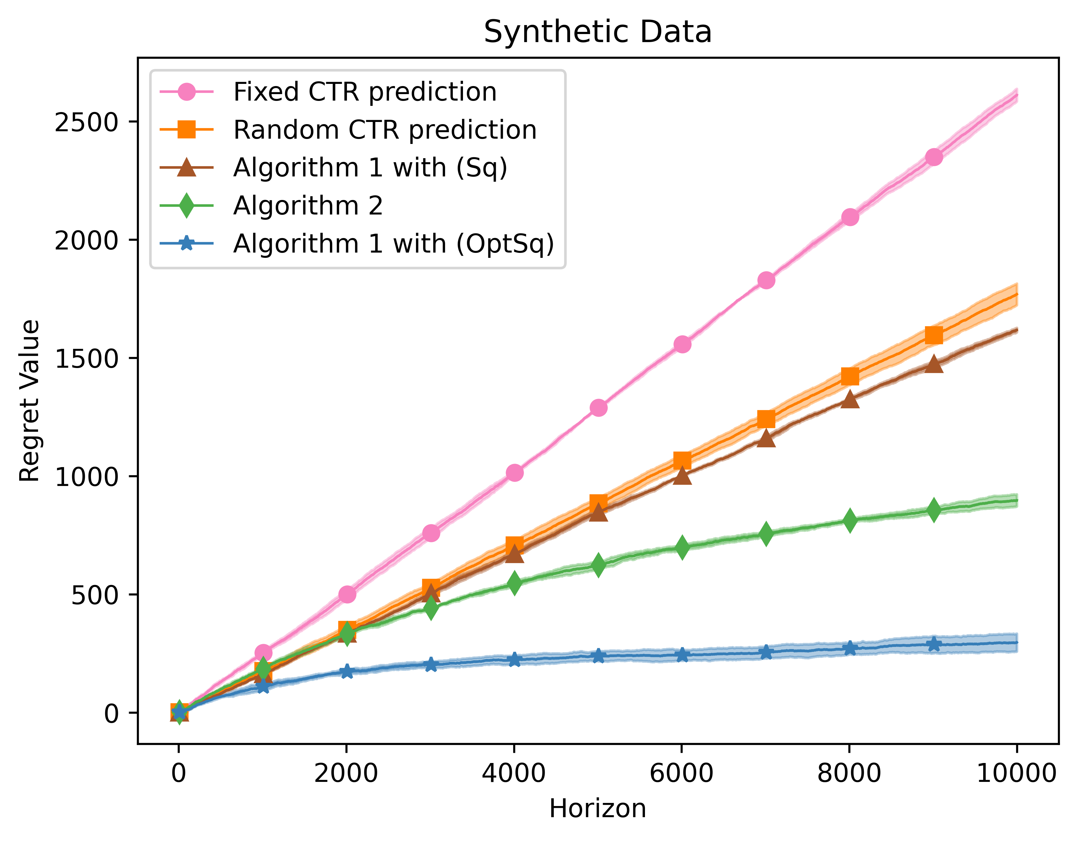
Figure 1: Performance of different algorithms on synthetic data

Appendix A Omitted Proofs in Section 3

Proof of Theorem 1.

According to standard analysis of exponential weight (see for example [Wei et al., 2020, Lemma 14]), we have for any $f_{0}\in{\mathcal{F}}$:

$$\left\langle{q_{t}-e_{f_{0}},\widehat{\ell}_{t}}\right\rangle \leq\frac{1}{\eta}D(e_{f_{0}},q_{t})-\frac{1}{\eta}D(e_{f_{0}},q_{t+1})+\frac{\eta}{2}\sum_{f\in{\mathcal{F}}}q_{t,f}\widehat{\ell}_{t,f}^{2},$$

where $D(u,v)=\sum_{f\in{\mathcal{F}}}u_{f}\log\frac{u_{f}}{v_{f}}$ is the KL divergence between $u$ and $v$. Taking summation over $t\in[T]$, we have with $i_{t,f}=\operatorname*{argmax}_{i}b_{t,i}f(x_{t},i)$:

$$\sum_{t=1}^{T}\left\langle{q_{t}-e_{f_{0}},\widehat{\ell}_{t}}\right\rangle$$

$$\leq\frac{D(e_{f_{0}},q_{1})}{\eta}+\frac{\eta}{2}\sum_{t=1}^{T}\sum_{f\in{\mathcal{F}}}q_{t,f}\widehat{\ell}_{t,f}^{2}$$

$$=\frac{D(e_{f_{0}},q_{1})}{\eta}+\frac{\eta}{2}\sum_{t=1}^{T}\sum_{i\in[N_{t}]}\sum_{f\in{\mathcal{F}},i=i_{t,f}}q_{t,f}\widehat{\ell}_{t,f}^{2}$$

$$=\frac{D(e_{f_{0}},q_{1})}{\eta}+\frac{\eta}{2}\sum_{t=1}^{T}\sum_{i\in[N_{t}]}\sum_{f\in{\mathcal{F}},i=i_{t,f}}\frac{q_{t,f}}{p_{t,i}^{2}}\left(1-c_{t}\cdot\frac{{\mathrm{smax}}_{j}b_{t,j}f(x_{t},j)}{f(x_{t},i_{t,f})}\right)^{2}\cdot\mathbbm{1}\{i_{t}=i\}$$

$$\leq\frac{D(e_{f_{0}},q_{1})}{\eta}+\frac{\eta}{2}\sum_{t=1}^{T}\sum_{i\in[N_{t}]}\sum_{f\in{\mathcal{F}},i=i_{t,f}}\frac{q_{t,f}\mathbbm{1}\{i_{t}=i\}}{p_{t,i}^{2}}$$

$$=\frac{D(e_{f_{0}},q_{1})}{\eta}+\frac{\eta}{2}\sum_{t=1}^{T}\sum_{i\in[N_{t}]}\frac{\mathbbm{1}\{i_{t}=i\}}{p_{t,i}} p_{t,i}=\sum_{f\in{\mathcal{F}}:i=i_{t,f}}q_{t,f}$$ ()

where the inequality is because ${\mathrm{smax}}_{j}b_{t,j}f(x_{t},j)\leq b_{t,i_{t,f}}f(x_{t},i_{t,f})$ and thus $1-c_{t}\cdot\frac{{\mathrm{smax}}_{j}b_{t,j}f(x_{t},j)}{f(x_{t},i_{t,f})}\in[0,1]$. Taking expectation over both sides and noticing

$$\mathbb{E}\left[\frac{\mathbbm{1}\{i_{t}=i\}}{p_{t,i}}\right]=\mathbb{E}\left[\frac{p_{t,i}}{p_{t,i}}\right]=1,$$

$$\mathbb{E}\left[\widehat{\ell}_{t,f}\right] =\mathbb{E}\left[\frac{\mathbbm{1}\{i_{t}=i_{t,f}\}}{p_{t,i_{t}}}\left(1-\rho_{t,i_{t,f}}\cdot\frac{{\mathrm{smax}}_{j}b_{t,j}f(x_{t},j)}{f(x_{t},i_{t,f})}\right)\right]$$

$$=1-\rho_{t,i_{t,f}}\cdot\frac{{\mathrm{smax}}_{j}b_{t,j}f(x_{t},j)}{f(x_{t},i_{t,f})}$$

$$=1-f^{*}(x_{t},i_{t,f})\cdot\frac{{\mathrm{smax}}_{j}b_{t,j}f(x_{t},j)}{f(x_{t},i_{t,f})},$$

we obtain

$$\begin{split}&\mathbb{E}\left[\sum_{t=1}^{T}f^{*}(x_{t},i_{t,f_{0}})\cdot\frac{{\mathrm{smax}}_{j}b_{t,j}f_{0}(x_{t},j)}{f_{0}(x_{t},i_{t,f_{0}})}-\sum_{t=1}^{T}f^{*}(x_{t},i_{t,f_{t}})\cdot\frac{{\mathrm{smax}}_{j}b_{t,j}f_{t}(x_{t},j)}{f_{t}(x_{t},i_{t,f_{t}})}\right]\\ &=\mathbb{E}\left[\sum_{t=1}^{T}f^{*}(x_{t},i_{t,f_{0}})\cdot\frac{{\mathrm{smax}}_{j}b_{t,j}f_{0}(x_{t},j)}{f_{0}(x_{t},i_{t,f_{0}})}-\sum_{t=1}^{T}c_{t}d_{t}\right]\leq\frac{D(e_{f_{0}},q_{1})}{\eta}+\frac{\eta}{2}\sum_{t=1}^{T}N_{t}.\end{split}$$ (5)

Picking $f_{0}=f^{*}$, which is in the class ${\mathcal{F}}$ by Assumption 1, the left-hand side above becomes exactly the expected regret $\mathbb{E}\left[\text{\rm Reg}\right]$. Finally, since $q_{1}$ is a uniform distribution over ${\mathcal{F}}$, we know that $D(e_{f^{*}},q_{1})=\log|{\mathcal{F}}|$, and picking $\eta=\sqrt{\frac{\log|{\mathcal{F}}|}{\sum_{t=1}^{T}N_{t}}}$ then leads to the claimed regret bound. ∎

Proof of Corollary 1.

For any $u\in[0,1]$, define $\lfloor u\rfloor_{T}=\frac{1}{T}\lfloor Tu\rfloor$. Since we consider the non-contextual setting, we have $\rho=\rho_{t}$ for all $t\in[T]$ and the policy $f\in\widehat{{\mathcal{F}}}$ can be represented as a vector in $[0,1]^{N}$. To show that Algorithm 1 guarantees $\mathcal{O}(N\sqrt{T\log N})$ regret, let $\widehat{f}^{*}=(\lfloor\rho_{1}\rfloor_{T},\dots,\lfloor\rho_{N}\rfloor_{T})\in\widehat{{\mathcal{F}}}$. Using Eq. (5) and picking $f_{0}=\widehat{f}^{*}$, we know that

$$\mathbb{E}\left[\sum_{t=1}^{T}\rho_{i_{t,\widehat{f}^{*}}}\cdot\frac{b_{t,j_{t,\widehat{f}^{*}}}\widehat{f}^{*}_{j_{t,\widehat{f}^{*}}}}{\widehat{f}^{*}_{i_{t,\widehat{f}^{*}}}}-\sum_{t=1}^{T}c_{t}d_{t}\right]\leq\mathcal{O}\left(\frac{N\log T}{\eta}\right)+\frac{\eta NT}{2},$$

where $i_{t,\rho}=\operatorname*{argmax}_{i}b_{t,i}\rho_{t,i}$ and $j_{t,\rho}=\operatorname*{argsmax}_{i}b_{t,i}\rho_{t,i}$. It remains to argue that the first term above is close to $\sum_{t=1}^{T}{\mathrm{smax}}_{i}b_{t,i}\rho_{i}$, the revenue of the oracle strategy. To this end, for each time $t$ we consider two cases depending on whether $\widehat{f}^{*}$ and $\rho$ selects the same winner. If $i_{t,\widehat{f}^{*}}=i_{t,\rho}$, we have

$$\rho_{i_{t,\widehat{f}^{*}}}\cdot\frac{b_{t,j_{t,\widehat{f}^{*}}}\widehat{f}^{*}_{j_{t,\widehat{f}^{*}}}}{\widehat{f}^{*}_{i_{t,\widehat{f}^{*}}}} \geq b_{t,j_{t,\widehat{f}^{*}}}\widehat{f}^{*}_{j_{t,\widehat{f}^{*}}} \widehat{f}^{*}_{i}=\lfloor\rho_{i}\rfloor_{T}\leq\rho_{i}$$ (since )

$$\geq b_{t,j_{t,\rho}}\widehat{f}^{*}_{j_{t,\rho}} b_{t,j_{t,\widehat{f}^{*}}}\widehat{f}^{*}_{j_{t,\widehat{f}^{*}}}={\mathrm{smax}}_{i}b_{t,i}\widehat{f}^{*}_{i} j_{t,\rho}\neq i_{t,\rho}=i_{t,\widehat{f}^{*}}$$ (since and )

$$\geq b_{t,j_{t,\rho}}\rho_{j_{t,\rho}}-\frac{1}{T} \widehat{f}^{*}_{i}=\lfloor\rho_{i}\rfloor_{T}\geq\rho_{i}-\frac{1}{T}$$ (since )

$$={\mathrm{smax}}_{i}b_{t,i}\rho_{i}-\frac{1}{T}.$$

Otherwise, we know that $b_{t,j_{t,\widehat{f}^{*}}}\widehat{f}^{*}_{j_{t,\widehat{f}^{*}}}\geq b_{t,i_{t,\rho}}\widehat{f}^{*}_{i_{t,\rho}}\geq b_{t,i_{t,\rho}}\rho_{i_{t,\rho}}-\frac{1}{T}\geq{\mathrm{smax}}_{i}b_{t,i}\rho_{i}-\frac{1}{T}$. Combining both cases, we know that

$$\mathbb{E}\left[\sum_{t=1}^{T}{\mathrm{smax}}_{i}b_{t,i}\rho_{i}-\sum_{t=1}^{T}c_{t}d_{t}\right]\leq\mathbb{E}\left[\sum_{t=1}^{T}\rho_{i_{t,\widehat{f}^{*}}}\cdot\frac{b_{t,j_{t,\widehat{f}^{*}}}\widehat{f}^{*}_{j_{t,\widehat{f}^{*}}}}{\widehat{f}^{*}_{i_{t,\widehat{f}^{*}}}}-\sum_{t=1}^{T}c_{t}d_{t}\right]+1$$

$$\leq\mathcal{O}\left(\frac{N\log T}{\eta}\right)+\frac{\eta NT}{2}+1.$$

Picking $\eta=\sqrt{\frac{\log T}{T}}$ achieves the claimed bound. ∎

Proof of Theorem 1.

The proof follows the idea of the lower bound construction in multi-armed bandits. Consider an instance of the auction problem with $N_{t}=N$ bidders and CTR $\{\rho_{i}\}_{i=1}^{N}$. The bid vector $b_{t}$ at each round $t$ is $\bm{1}$. Denote $\rho^{(i,j)}$ $(i\neq j)$ to be the environment where $\rho_{k}^{(i,j)}=\frac{1}{2}$ for all $k\in[N]\backslash\{i,j\}$ and $\rho_{i}^{(i,j)}=\rho_{j}^{(i,j)}=\frac{1}{2}+\varepsilon$ for some $\varepsilon>0$ to be specified later. We also denote $\rho^{(0)}$ to be the environment where $\rho^{(0)}_{i}=\frac{1}{2}$ for all $i\in[N]$.

Consider the environment ${\mathcal{E}}$ where $\rho$ is uniformly drawn from the $\frac{N(N-1)}{2}$ environments $\{\rho^{(i,j)}\}_{i\neq j,i,j\in[n]}$. For notational convenience, we denote $\mathbb{E}_{i,j}[\cdot]$ ($\mathbb{E}_{0}$) to be $\mathbb{E}_{\rho^{(i,j)}}[\cdot]$ ($\mathbb{E}_{\rho^{(0)}}$). Let $n_{i}$ be the number of rounds ad $i$ is selected as the winner (via picking an estimated CTR). Since the payment per click can not exceed the bid $1$ according to the auction design, the expected revenue of the learner is at most the CTR of the winning ad. In addition, the benchmark revenue in environment $\rho^{(i,j)}$ is $(\frac{1}{2}+\varepsilon)T$ by picking the estimated CTR as the true CTR. Therefore, the expected regret with respect to environment ${\mathcal{E}}$ is lower bounded as follows:

$$\mathbb{E}_{{\mathcal{E}}}[\text{\rm Reg}] \geq\frac{2}{N(N-1)}\sum_{i\neq j}\mathbb{E}_{i,j}\left[\left(\frac{1}{2}+\varepsilon\right)T-\frac{1}{2}\sum_{k\neq i,j}n_{k}-\left(\frac{1}{2}+\varepsilon\right)(n_{i}+n_{j})\right]$$

$$=\frac{2}{N(N-1)}\sum_{i\neq j,i,j\in[N]}\mathbb{E}_{i,j}\left[\varepsilon(T-n_{i}-n_{j})\right],$$ (6)

where the last equality uses the fact that $\sum_{i=1}^{N}n_{i}=T$. According to Exercise 15.2.(a) of [Lattimore and Szepesvári, 2020], we have

$$\mathbb{E}_{i,j}[n_{i}+n_{j}]\leq\mathbb{E}_{0}[n_{i}+n_{j}]+T\sqrt{\frac{1}{4}\varepsilon^{2}\mathbb{E}_{0}[n_{i}+n_{j}]}.$$

Taking summation over all $i\neq j$, $i,j\in[N]$, we obtain that

$$\sum_{i\neq j,i,j\in[N]}\mathbb{E}_{i,j}[n_{i}+n_{j}] \leq\sum_{i\neq j,i,j\in[N]}\mathbb{E}_{0}[n_{i}+n_{j}]+\frac{T\varepsilon}{2}\sum_{i\neq j,i,j\in[N]}\sqrt{\mathbb{E}_{0}[n_{i}+n_{j}]}$$

$$\leq(N-1)\sum_{i=1}^{N}\mathbb{E}_{0}[n_{i}]+\frac{T\varepsilon}{2}(N-1)\sum_{i=1}^{N}\sqrt{\mathbb{E}_{0}[n_{i}]}$$

$$\leq(N-1)T+\frac{T\varepsilon(N-1)}{2}\sqrt{NT},$$ (7)

where the second inequality uses $\sqrt{a+b}\leq\sqrt{a}+\sqrt{b}$ and the third inequality is due to Cauchy-Schwarz inequality.

Applying Eq. (7) to Eq. (6), we obtain that

$$\mathbb{E}_{{\mathcal{E}}}[\text{\rm Reg}] \geq\varepsilon T-\frac{2\varepsilon}{N(N-1)}\cdot\left[(N-1)T+\frac{T\varepsilon(N-1)}{2}\sqrt{NT}\right]$$

$$=\varepsilon T-\frac{2\varepsilon T}{N}-\varepsilon^{2}N^{-\frac{1}{2}}T^{\frac{3}{2}}$$

$$\geq\frac{1}{3}\varepsilon T-\varepsilon^{2}N^{-\frac{1}{2}}T^{\frac{3}{2}}. N\geq 3$$ ()

Picking $\varepsilon=\frac{1}{4}\sqrt{\frac{N}{T}}$ leads to $\mathbb{E}_{{\mathcal{E}}}[\text{\rm Reg}]\geq\frac{1}{48}\sqrt{NT}$. Therefore, there exists one environment among $\{\rho^{(i,j)}\}_{i\neq j,i,j\in[N]}$ such that $\mathbb{E}_{i,j}[\text{\rm Reg}]\geq\frac{1}{48}\sqrt{NT}$, which finishes the proof. ∎

Appendix B Omitted Proofs in Section 4

Proof of Theorem 4.

Let $i_{t}^{*}=\operatorname*{argmax}_{i\in[N_{t}]}b_{t,i}\rho_{t,i}$, $j_{t}^{*}=\operatorname*{argsmax}_{j\in[N_{t}]}b_{t,i}\rho_{t,i}$, $i_{t,f}=\operatorname*{argmax}_{i\in[N_{t}]}b_{t,i}f(x_{t},i)$, and $j_{t,f}=\operatorname*{argsmax}_{i\in[N_{t}]}b_{t,i}f(x_{t},i)$. Also recall the notation $i_{t}=\operatorname*{argmax}_{i\in[N_{t}]}b_{t,i}\widetilde{\rho}_{t,i}$ and $j_{t}=\operatorname*{argsmax}_{j\in[N_{t}]}b_{t,i}\widetilde{\rho}_{t,i}$. Then, we decompose the regret as follows:

$$\mathbb{E}\left[\text{\rm Reg}\right] =\mathbb{E}\left[\sum_{t=1}^{T}{\mathrm{smax}}_{i\in[N_{t}]}\;b_{t,i}\rho_{t,i}-\sum_{t=1}^{T}c_{t}d_{t}\right]$$

$$=\mathbb{E}\left[\sum_{t=1}^{T}\rho_{t,j_{t}^{*}}b_{t,j_{t}^{*}}-\sum_{t=1}^{T}\frac{\widetilde{\rho}_{t,j_{t}}b_{t,j_{t}}}{\widetilde{\rho}_{t,i_{t}}}\rho_{t,i_{t}}\right]$$

$$=\mathbb{E}\left[\sum_{t=1}^{T}\mathbb{E}_{i_{t},j_{t}}\left[\frac{\widetilde{\rho}_{t,j_{t}}b_{t,j_{t}}}{\widetilde{\rho}_{t,i_{t}}}\left(\widetilde{\rho}_{t,i_{t}}-\rho_{t,i_{t}}\right)\right]\right]-\mathbb{E}\left[\sum_{t=1}^{T}\left(\widetilde{\rho}_{t,j_{t}}b_{t,j_{t}}-\rho_{t,j_{t}^{*}}b_{t,j_{t}^{*}}\right)\right]$$

$$=\mathbb{E}\left[\sum_{t=1}^{T}\mathbb{E}_{f\sim q_{t}}\left[\frac{f(x_{t},j_{t,f})b_{t,j_{t,f}}}{f(x_{t},i_{t,f})}\left(f(x_{t},i_{t,f})-f^{*}(x_{t},i_{t,f})\right)\right]\right]$$

$$\qquad-\mathbb{E}\left[\sum_{t=1}^{T}\underbrace{\left(f_{t}(x_{t},j_{t})b_{t,j_{t}}-f^{*}(x_{t},j_{t}^{*})b_{t,j_{t}^{*}}\right)}_{\triangleq\mathrm{FG}_{t}}\right]$$

$$\leq\mathbb{E}\left[\sum_{t=1}^{T}\mathbb{E}_{f\sim q_{t}}\left[|f(x_{t},i_{t,f})-f^{*}(x_{t},i_{t,f})|\right]\right]-\mathbb{E}\left[\sum_{t=1}^{T}\mathrm{FG}_{t}\right]$$

where the inequality is because $\frac{f(x_{t},j_{t,f})b_{t,j_{t,f}}}{f(x_{t},i_{t,f})}\leq b_{t,i_{t,f}}\leq 1$. Note that the “Feel-Good” term $\mathrm{FG}_{t}$ is the difference between what $f_{t}$ believes its payment is in its predicted world and that of the perfect predictor $f^{*}$. We now analyze the other term for each time $t$, which can be written as:

$$\sum_{i\in[N_{t}]:p_{t,i}\neq 0}\mathbb{E}_{f\sim q_{t}}\left[\mathbbm{1}\{i_{t,f}=i\}|f(x_{t},i)-f^{*}(x_{t},i)|\right].$$

where $p_{t,i}$ is the probability of $i_{t}$ being $i$. Now consider a fixed $i$. We have for any $\mu>0$,

$$\mathbb{E}_{f\sim q_{t}}\left[\mathbbm{1}\{i_{t,f}=i\}|f(x_{t},i)-f^{*}(x_{t},i)|\right]$$

$$\leq\mathbb{E}_{f\sim q_{t}}\left[\frac{\mathbbm{1}\{i_{t,f}=i\}}{4\mu p_{t,i}}+\mu p_{t,i}\left(f(x_{t},i)-f^{*}(x_{t},i)\right)^{2}\right]$$ (AM-GM inequality)

$$=\frac{1}{4\mu}+\mu p_{t,i}\mathbb{E}_{f\sim q_{t}}\left[\left(f(x_{t},i)-f^{*}(x_{t},i)\right)^{2}\right], p_{t,i}=\mathbb{E}_{f\sim q_{t}}[\mathbbm{1}\{i_{t,f}=i\}]$$ ()

which, after taking the summation over $i$, becomes

$$\frac{N_{t}}{4\mu}+\mu\mathbb{E}_{i_{t}\sim p_{t}}\mathbb{E}_{f\sim q_{t}}\left[\left(f(x_{t},i_{t})-f^{*}(x_{t},i_{t})\right)^{2}\right]$$

(note the important decoupling effect here: $f$ is not $f_{t}$). With notation $\mathrm{LS}_{t}\triangleq(f(x_{t},i_{t})-f^{*}(x_{t},i_{t}))^{2}$ (“Least Squares”), we have thus shown for any $\mu>0$:

$$\mathbb{E}[\text{\rm Reg}]\leq\frac{1}{4\mu}\sum_{t=1}^{T}N_{t}+\mu\mathbb{E}\left[\sum_{t=1}^{T}\mathbb{E}_{i_{t}\sim p_{t}}\mathbb{E}_{f\sim q_{t}}[\mathrm{LS}_{t}]\right]-\mathbb{E}\left[\sum_{t=1}^{T}\mathbb{E}_{f_{t}\sim q_{t}}[\mathrm{FG}_{t}]\right].$$ (8)

Next, using the fact that $c_{t}$ is a Bernoulli random variable with mean $f^{*}(x_{t},i_{t})$ and following a similar analysis of Lemma $4$ in [Zhang, 2022], we can show that

$$\frac{1}{16\eta}\mathbb{E}_{f\sim q_{t}}[\mathrm{LS}_{t}]-\mathbb{E}_{f_{t}\sim q_{t}}[\mathrm{FG}_{t}]\leq-\frac{1}{\eta}\log\mathbb{E}_{c_{t}|x_{t},i_{t}}\mathbb{E}_{f\sim q_{t}}\left[\exp\left(-\eta\left(\widehat{\ell}_{t,f}-\widehat{\ell}_{t,f^{*}}\right)\right)\right]+4\eta,$$ (9)

with $\widehat{\ell}_{t,f}$ defined as the $\mathsf{(OptSq)}$ option shown in Algorithm 1. For completeness, we include the proof of Eq. (9) in Lemma B.1. Comparing Eq. (8) and Eq. (9) naturally suggests picking $\mu=\frac{1}{16\eta}$, so that

$$\mathbb{E}[\text{\rm Reg}]\leq 4\eta\sum_{t=1}^{T}N_{t}+4T\eta-\frac{1}{\eta}\sum_{t=1}^{T}\log\mathbb{E}_{c_{t}|x_{t},i_{t}}\mathbb{E}_{f\sim q_{t}}\left[\exp\left(-\eta\left(\widehat{\ell}_{t,f}-\widehat{\ell}_{t,f^{*}}\right)\right)\right].$$ (10)

Note that the analysis so far holds for any $q_{t}$. To complete the proof, we now use the specific form of $q_{t}$ defined in Algorithm 1: $q_{t,f}\propto\exp\left(-\eta\sum_{s=1}^{t-1}\widehat{\ell}_{s,f}\right)$. Using standard analysis of the multiplicative weight update, we show in Lemma B.2 the following:

$$-\mathbb{E}\left[\mathbb{E}_{i_{t}}\log\mathbb{E}_{c_{t}|x_{t},i_{t}}\;\mathbb{E}_{f\sim q_{t}}\;\left[\exp(-\eta(\widehat{\ell}_{t,f}-\widehat{\ell}_{t,f^{*}}))\right]\right]\leq Z_{t}-Z_{t-1},$$ (11)

where $Z_{t}=-\mathbb{E}\left[\log\mathbb{E}_{f\sim q_{1}}\exp\left(-\eta\sum_{\tau=1}^{t}\left(\widehat{\ell}_{t,f}-\widehat{\ell}_{t,f^{*}}\right)\right)\right]$. Combining this fact with Eq. (10), we arrive at

$$\mathbb{E}[\text{\rm Reg}] \leq 4\eta\sum_{t=1}^{T}N_{t}+4T\eta+\frac{1}{\eta}\sum_{t=1}^{T}(Z_{t}-Z_{t-1})$$

$$\leq 4\eta\sum_{t=1}^{T}N_{t}+4T\eta+\frac{Z_{T}}{\eta}, Z_{0}=0$$ (telescoping and )

which finishes the proof. ∎

Lemma B.1.

Suppose that $\eta\leq 1$. For any distribution $q_{t}$ over ${\mathcal{F}}$ and $b_{t}\in[0,1]^{N}$, we have

$$\frac{1}{16\eta}\mathbb{E}_{f\sim q_{t}}[\mathrm{LS}_{t}]-\mathbb{E}_{f_{t}\sim q_{t}}[\mathrm{FG}_{t}]\leq-\frac{1}{\eta}\log\mathbb{E}_{c_{t}|x_{t},i_{t}}\mathbb{E}_{f\sim q_{t}}\exp\left(-\eta\left(\widehat{\ell}_{t,f}-\widehat{\ell}_{t,f^{*}}\right)\right)+4\eta,$$

where $\mathrm{LS}_{t}$ and $\mathrm{FG}_{t}$ are defined in the proof of Theorem 4, and $\widehat{\ell}_{t,f}$ is defined in the $\mathsf{(OptSq)}$ option of Eq. (2).

Proof.

Since $c_{t}\in\{0,1\}$ is a Bernoulli random variable with mean $f^{*}(x_{t},i_{t})$, $c_{t}$ satisfies the following sub-Gaussian random variable property: for any $\rho$,

$$\mathbb{E}_{c_{t}|x_{t},i_{t}}\left[\exp\left(\rho\left(c_{t}-f^{*}(x_{t},i_{t})\right)\right)\right]\leq\exp\left(\frac{\rho^{2}}{8}\right).$$

Let $\varepsilon_{t}=c_{t}-f^{*}(x_{t},i_{t})$. For any $f$, setting $\rho=-\frac{1}{2}(f^{*}(x_{t},i_{t})-f(x_{t},i_{t}))$, we thus have

$$\mathbb{E}_{c_{t}|x_{t},i_{t}}\exp\left(-\frac{1}{2}\varepsilon_{t}\left(f^{*}(x_{t},i_{t})-f(x_{t},i_{t})\right)\right)\leq\exp\left(\frac{1}{32}\mathrm{LS}_{t}\right).$$ (12)

On the other hand, consider the following equalities:

$$-\eta\left(\widehat{\ell}_{t,f}-\widehat{\ell}_{t,f^{*}}\right)$$

$$=-\frac{1}{4}(f(x_{t},i_{t})-c_{t})^{2}+\frac{1}{4}(f^{*}(x_{t},i_{t})-c_{t})^{2}+\eta\cdot{\mathrm{smax}}_{j}b_{t,j}f(x_{t},j)-\eta\cdot{\mathrm{smax}}_{j}b_{t,j}f^{*}(x_{t},j)$$

$$=-\frac{1}{4}(\varepsilon_{t}+f^{*}(x_{t},i_{t})-f(x_{t},i_{t}))^{2}+\frac{1}{4}\varepsilon_{t}^{2}+\eta\cdot{\mathrm{smax}}_{j}b_{t,j}f(x_{t},j)-\eta\cdot{\mathrm{smax}}_{j}b_{t,j}f^{*}(x_{t},j)$$

$$=-\frac{1}{2}\varepsilon_{t}(f^{*}(x_{t},i_{t})-f(x_{t},i_{t}))-\frac{1}{4}\mathrm{LS}_{t}+\eta\mathrm{FG}_{t}(f),$$

where we define $\mathrm{FG}_{t}(f)={\mathrm{smax}}_{j}(f(x_{t},j)b_{t,j})-{\mathrm{smax}}_{j}(f^{*}(x_{t},j)b_{t,j})$ (so $\mathrm{FG}_{t}=\mathrm{FG}_{t}(f_{t})$). Combining the above with Eq. (12), we obtain

$$\mathbb{E}_{c_{t}|x_{t},i_{t}}\left[\exp\left(-\eta\left(\widehat{\ell}_{t,f}-\widehat{\ell}_{t,f^{*}}\right)\right)\right]\leq\exp\left(-\frac{7}{32}\mathrm{LS}_{t}+\eta\mathrm{FG}_{t}(f)\right).$$

This further shows:

$$\log\mathbb{E}_{f\sim q_{t}}\left[\mathbb{E}_{c_{t}|x_{t},i_{t}}\left[\exp\left(-\eta\left(\widehat{\ell}_{t,f}-\widehat{\ell}_{t,f^{*}}\right)\right)\right]\right]$$

$$\leq\log\mathbb{E}_{f\sim q_{t}}\left[\exp\left(-\frac{7}{32}\mathrm{LS}_{t}+\eta\mathrm{FG}_{t}(f)\right)\right]$$

$$\leq\frac{1}{2}\log\mathbb{E}_{f\sim q_{t}}\left[\exp\left(-\frac{7}{16}\mathrm{LS}_{t}\right)\right]+\frac{1}{2}\log\mathbb{E}_{f\sim q_{t}}\left[\exp(2\eta\mathrm{FG}_{t}(f))\right],$$ (13)

where the last inequality is due to Cauchy-Schwarz inequality. For the first term, using the facts $0\leq\mathrm{LS}_{t}\leq 1$ and $e^{x}\leq 1+x+\frac{x^{2}}{2}$ for $x\leq 0$, we know

$$\mathbb{E}_{f\sim q_{t}}\left[\exp\left(-\frac{7}{16}\mathrm{LS}_{t}\right)\right]\leq 1-\frac{7}{16}\mathbb{E}_{f\sim q_{t}}[\mathrm{LS}_{t}]+\frac{49}{256}\mathbb{E}_{f\sim q_{t}}[\mathrm{LS}_{t}^{2}]\leq 1-\frac{1}{8}\mathbb{E}_{f\sim q_{t}}[\mathrm{LS}_{t}],$$

where the last inequality is because $\mathrm{LS}_{t}^{2}\leq\mathrm{LS}_{t}$. Further using $\log(1+x)\leq x$ gives

$$\frac{1}{2}\log\mathbb{E}_{f\sim q_{t}}\left[\exp\left(-\frac{7}{16}\mathrm{LS}_{t}\right)\right]\leq\frac{1}{2}\log\left(1-\frac{1}{8}\mathbb{E}_{f\sim q_{t}}[\mathrm{LS}_{t}]\right)\leq-\frac{1}{16}\mathbb{E}_{f\sim q_{t}}[\mathrm{LS}_{t}].$$ (14)

Moreover, since $\eta\leq 1$ and $|\mathrm{FG}_{t}(f)|\leq 1$, using $e^{x}\leq 1+x+2x^{2}$ for $x\leq 2$, we have

$$\frac{1}{2}\log\mathbb{E}_{f\sim q_{t}}\left[\exp(2\eta\mathrm{FG}_{t}(f))\right] \leq\frac{1}{2}\log\left(1+2\eta\mathbb{E}_{f\sim q_{t}}[\mathrm{FG}_{t}(f)]+2(2\eta)^{2}\right)$$

$$\leq\eta\mathbb{E}_{f\sim q_{t}}[\mathrm{FG}_{t}(f)]+4\eta^{2} \log(1+x)\leq x$$ ()

$$=\eta\mathbb{E}_{f_{t}\sim q_{t}}[\mathrm{FG}_{t}]+4\eta^{2}. f_{t} q_{t}$$ ( is drawn from )

Plugging the last bound and Eq. (14) into Eq. (13) and rearranging finishes the proof. ∎

Lemma B.2.

Algorithm 1 guarantees that for each $t\in[T]$,

$$-\mathbb{E}\left[\mathbb{E}_{i_{t}\sim p_{t}}\log\mathbb{E}_{c_{t}|x_{t},i_{t}}\;\mathbb{E}_{f\sim q_{t}}\;\left[\exp(-\eta(\widehat{\ell}_{t,f}-\widehat{\ell}_{t,f^{*}}))\right]\right]\leq Z_{t}-Z_{t-1},$$

where $Z_{t}=-\mathbb{E}\left[\log\mathbb{E}_{f\sim q_{1}}\left[\exp\left(-\eta\sum_{\tau=1}^{t}\left(\widehat{\ell}_{t,f}-\widehat{\ell}_{t,f^{*}}\right)\right)\right]\right]$.

Proof.

Let $W_{t,f}\triangleq\exp\left(-\eta\sum_{\tau=1}^{t}\left(\widehat{\ell}_{t,f}-\widehat{\ell}_{t,f^{*}}\right)\right)$. According to Algorithm 1, we know that

$$q_{t,f}=\frac{\exp\left(-\eta\sum_{\tau=1}^{t-1}\widehat{\ell}_{\tau,f}\right)}{\int_{f^{\prime}\in{\mathcal{F}}}\exp\left(-\eta\sum_{\tau=1}^{t-1}\widehat{\ell}_{\tau,f^{\prime}}\right)df^{\prime}}=\frac{W_{t-1,f}}{\int_{f^{\prime}\in{\mathcal{F}}}W_{t-1,f^{\prime}}df^{\prime}}.$$

Then, according to the definition of $Z_{t}$, we have

$$Z_{t-1}-Z_{t}$$

$$=\mathbb{E}\left[\log\frac{\int_{f\in{\mathcal{F}}}W_{t,f}df}{\int_{f\in{\mathcal{F}}}\;W_{t-1,f}df}\right]$$

$$=\mathbb{E}\left[\log\frac{\int_{f\in{\mathcal{F}}}\;W_{t-1,f}\exp(-\eta(\widehat{\ell}_{t,f}-\widehat{\ell}_{t,f^{*}}))df}{\int_{f\in{\mathcal{F}}}W_{t-1,f}df}\right]$$

$$=\mathbb{E}\left[\log\mathbb{E}_{f\sim q_{t}}\left[\exp(-\eta(\widehat{\ell}_{t,f}-\widehat{\ell}_{t,f^{*}})\right]\right]$$

$$\leq\mathbb{E}\left[\mathbb{E}_{i_{t}\sim p_{t}}\log\mathbb{E}_{c_{t}|x_{t},i_{t}}\mathbb{E}_{f\sim q_{t}}\left[\exp(-\eta(\widehat{\ell}_{t,f}-\widehat{\ell}_{t,f^{*}})\right]\right],$$

where the last inequality is due to Jensen’s inequality. Rearranging the terms finishes the proof. ∎

Proof of Corollary 4.

To show that $Z_{T}=\mathcal{O}(\alpha+d\log BT)$, we consider a small cube around the true parameter $\theta^{*}$: $\Omega_{T}=\{\theta:\|\theta-\theta^{*}\|_{\infty}\leq\frac{1}{T}\}$. Since ${\mathcal{F}}$ is $\alpha$-Lipschitz with respect to $\|\cdot\|_{\infty}$, we know that $\|f_{\theta}-f_{\theta^{*}}\|_{\infty}\leq\frac{\alpha}{T}$. Therefore, for any $\theta\in\Omega_{T}$,

$$-\eta(\widehat{\ell}_{t,f_{\theta}}-\widehat{\ell}_{t,f_{\theta^{*}}})$$

$$=-\frac{1}{4}(f_{\theta}(x_{t},i_{t})-c_{t})^{2}+\frac{1}{4}(f_{\theta^{*}}(x_{t},i_{t})-c_{t})^{2}$$

$$\qquad+\eta\cdot{\mathrm{smax}}_{j}b_{t,j}f_{\theta}(x_{t},j)-\eta\cdot{\mathrm{smax}}_{j}b_{t,j}f_{\theta^{*}}(x_{t},j)$$

$$\geq-\frac{1}{2}|f_{\theta}(x_{t},i_{t})-f_{\theta^{*}}(x_{t},i_{t})|+\eta\cdot{\mathrm{smax}}_{j}b_{t,j}f_{\theta}(x_{t},j)-\eta\cdot{\mathrm{smax}}_{j}b_{t,j}f_{\theta^{*}}(x_{t},j).$$ (15)

For the second and the third term, if $\operatorname*{argmax}_{i}b_{t,i}f_{\theta}(x_{t},i)=\operatorname*{argmax}_{i}b_{t,i}f_{\theta^{*}}(x_{t},i)$, let $j_{\theta^{*}}=\operatorname*{argsmax}_{j}b_{t,j}f_{\theta^{*}}(x_{t},j)$ and we know that

$${\mathrm{smax}}_{j}b_{t,j}f_{\theta}(x_{t},j)-{\mathrm{smax}}_{j}b_{t,j}f_{\theta^{*}}(x_{t},j)$$

$$\geq b_{t,j_{\theta^{*}}}f_{\theta}(x_{t},j_{\theta^{*}})-{\mathrm{smax}}_{j}b_{t,j}f_{\theta^{*}}(x_{t},j)$$

$$\geq-b_{t,j_{\theta^{*}}}|f_{\theta}(x_{t},j_{\theta^{*}})-f_{\theta^{*}}(x_{t},j_{\theta^{*}})|.$$

Otherwise, let $i_{\theta^{*}}=\operatorname*{argmax}_{i}b_{t,i}f_{\theta^{*}}(x_{t},i)$ and we know that

$${\mathrm{smax}}_{j}b_{t,j}f_{\theta}(x_{t},j)-{\mathrm{smax}}_{j}b_{t,j}f_{\theta^{*}}(x_{t},j)$$

$$\geq{\mathrm{smax}}_{j}b_{t,j}f_{\theta}(x_{t},j)-b_{t,i_{\theta^{*}}}f_{\theta^{*}}(x_{t},i_{\theta^{*}})$$

$$\geq b_{t,i_{\theta^{*}}}f_{\theta}(x_{t},i_{\theta^{*}})-b_{t,i_{\theta^{*}}}f_{\theta^{*}}(x_{t},i_{\theta^{*}})$$

$$\geq-b_{t,i_{\theta^{*}}}|f_{\theta}(x_{t},i_{\theta^{*}})-f_{\theta^{*}}(x_{t},i_{\theta^{*}})|.$$

Combining the two cases above and plugging them into Eq. (B), we obtain

$$-\eta(\widehat{\ell}_{t,f_{\theta}}-\widehat{\ell}_{t,f_{\theta^{*}}})\geq-\frac{\alpha}{2T}-\frac{\alpha\eta}{T}.$$

This means that

$$Z_{T} =-\mathbb{E}\left[\log\mathbb{E}_{f\sim q_{1}}\exp\left(-\eta\sum_{t=1}^{T}\left(\widehat{\ell}_{t,f_{\theta}}-\widehat{\ell}_{t,f_{\theta^{*}}}\right)\right)\right]$$

$$\leq-\mathbb{E}\left[\log\frac{1}{(BT)^{d}}\inf_{\theta\in\Omega_{T}}\exp\left(-\eta\sum_{t=1}^{T}\left(\widehat{\ell}_{t,f_{\theta}}-\widehat{\ell}_{t,f_{\theta^{*}}}\right)\right)\right]$$

$$\leq d\log BT+\frac{\alpha}{2}+\alpha\eta=\mathcal{O}(\alpha+d\log BT),$$

which finishes the proof. ∎

Appendix C Omitted Proofs in Section 5

Proof of Proposition 5.1.

By the definition of $\mathsf{dec}_{\gamma}$, we have

$$\mathbb{E}[\text{\rm Reg}]\leq\mathbb{E}\left[\gamma\sum_{t=1}^{T}(\rho_{t,i_{t}}-\widehat{\rho}_{t,i_{t}})^{2}+\sum_{t=1}^{T}\mathsf{dec}_{\gamma}(\widehat{\rho}_{t})\right].$$

It remains to notice that the first term is bounded by $\mathrm{\mathbf{Reg}}_{\mathsf{Sq}}$ under Assumption 2:

$$\mathrm{\mathbf{Reg}}_{\mathsf{Sq}}\geq\mathbb{E}\left[\sum_{t=1}^{T}\left(f_{t}(x_{t},i_{t})-c_{t}\right)^{2}-\sum_{t=1}^{T}\left(f^{*}(x_{t},i_{t})-c_{t}\right)^{2}\right]$$

$$=\mathbb{E}\left[\sum_{t=1}^{T}\left(f_{t}(x_{t},i_{t})-f^{*}(x_{t},i_{t})\right)\left(f_{t}(x_{t},i_{t})+f^{*}(x_{t},i_{t})-2c_{t})\right)\right]$$

$$=\mathbb{E}\left[\sum_{t=1}^{T}\left(f_{t}(x_{t},i_{t})-f^{*}(x_{t},i_{t})\right)^{2}\right] c_{t} f^{*}(x_{t},i_{t})$$ (the conditional expectation of is )

$$=\mathbb{E}\left[\sum_{t=1}^{T}(\rho_{t,i_{t}}-\widehat{\rho}_{t,i_{t}})^{2}\right].$$

This finishes the proof. ∎

Proof of Theorem 2.

Consider the $\varepsilon$-greedy strategy described above Theorem 2 and any $\rho,b\in[0,1]^{N}$. We have

$$\mathbb{E}_{\widetilde{\rho}\in Q}\Bigg{[}\left({\mathrm{smax}}_{i\in[N]}b_{i}\rho_{i}-\rho_{i^{*}}\frac{{\mathrm{smax}}_{j\in[N]}b_{j}\widetilde{\rho}_{j}}{\widetilde{\rho}_{i^{*}}}\right)-\gamma\left(\rho_{i^{*}}-\widehat{\rho}_{i^{*}}\right)^{2}\Bigg{]}$$

$$=\left({\mathrm{smax}}_{i\in[N]}b_{i}\rho_{i}-\mathbb{E}_{\widetilde{\rho}\in Q}\Bigg{[}\rho_{i^{*}}\frac{{\mathrm{smax}}_{j\in[N]}b_{j}\widetilde{\rho}_{j}}{\widetilde{\rho}_{i^{*}}}\Bigg{]}\right)-\gamma\sum_{i=1}^{N}p_{i}(\rho_{i}-\widehat{\rho}_{i})^{2}$$

$$\leq\left({\mathrm{smax}}_{i\in[N]}b_{i}\rho_{i}-(1-\varepsilon)\rho_{\widehat{i}^{*}}\frac{{\mathrm{smax}}_{j\in[N]}b_{j}\widehat{\rho}_{j}}{\widehat{\rho}_{\widehat{i}^{*}}}\right)-\gamma\sum_{i=1}^{N}p_{i}(\rho_{i}-\widehat{\rho}_{i})^{2}$$

$$\leq\left({\mathrm{smax}}_{i\in[N]}b_{i}\rho_{i}-\rho_{\widehat{i}^{*}}\frac{{\mathrm{smax}}_{j\in[N]}b_{j}\widehat{\rho}_{j}}{\widehat{\rho}_{\widehat{i}^{*}}}\right)-\gamma\sum_{i=1}^{N}p_{i}(\rho_{i}-\widehat{\rho}_{i})^{2}+\varepsilon$$ (16)

where in the first step we introduce the notation $p_{i}$ which is the probability of $i^{*}$ being $i$, in the second step we ignore the revenue obtained from exploration and use $\widehat{i}^{*}$ to denote $\operatorname*{argmax}_{i}b_{i}\widehat{\rho}_{i}$, and in the last step we use the fact $\frac{{\mathrm{smax}}_{j\in[N]}b_{j}\widehat{\rho}_{j}}{\widehat{\rho}_{\widehat{i}^{*}}}\leq 1$. We now make the following two observations for any $i\in[N]$, both due to AM-GM inequality and the fact $p_{i}\geq\varepsilon/N$:

$$\quad|b_{i}\rho_{i}-b_{i}\widehat{\rho}_{i}|-\frac{\gamma}{2}p_{i}(\rho_{i}-\widehat{\rho}_{i})^{2}\leq\frac{b_{i}^{2}}{2\gamma p_{i}}\leq\frac{N}{2\gamma\varepsilon},$$ (17)

$$\begin{split}\frac{{\mathrm{smax}}_{j\in[N]}b_{j}\widehat{\rho}_{j}}{\widehat{\rho}_{i}}|\rho_{\widehat{i}^{*}}-\widehat{\rho}_{\widehat{i}^{*}}|-\frac{\gamma}{2}p_{\widehat{i}^{*}}(\rho_{\widehat{i}^{*}}-\widehat{\rho}_{\widehat{i}^{*}})^{2}&\leq\frac{1}{2\gamma p_{\widehat{i}^{*}}}\left(\frac{{\mathrm{smax}}_{j\in[N]}b_{j}\widehat{\rho}_{j}}{\widehat{\rho}_{\widehat{i}^{*}}}\right)^{2}\\ &\leq\frac{b_{\widehat{i}^{*}}^{2}}{2\gamma p_{\widehat{i}^{*}}}\leq\frac{N}{2\gamma\varepsilon}.\end{split}$$ (18)

We are now ready to bound Eq. (16) by considering two cases: $\widehat{i}^{*}\neq j^{*}$ or $\widehat{i}^{*}=j^{*}$ where $j^{*}=\operatorname*{argsmax}_{i}b_{i}\rho_{i}$. In the first case ($\widehat{i}^{*}\neq j^{*}$), we use Eq. (17) with $i=j^{*}$ and Eq. (18) to continue to bound Eq. (16) as

$$b_{j^{*}}\widehat{\rho}_{j^{*}}-{\mathrm{smax}}_{j\in[N]}b_{j}\widehat{\rho}_{j}+\frac{N}{\gamma\varepsilon}+\varepsilon\leq\frac{N}{\gamma\varepsilon}+\varepsilon,$$

where the last step is because $j^{*}$ is not $\widehat{i}^{*}$ and thus $b_{j^{*}}\widehat{\rho}_{j^{*}}$ is not $\max_{j}b_{j}\widehat{\rho}_{j}$ and must be at most the second max. In the second case ($\widehat{i}^{*}=j^{*}$), we know $\widehat{i}^{*}\neq\operatorname*{argmax}_{i}b_{i}\rho_{i}\triangleq k$, and thus we first bound ${\mathrm{smax}}_{i\in[N]}b_{i}\rho_{i}$ by $b_{k}\rho_{k}$ and then apply Eq. (17) with $i=k$ and Eq. (18) to obtain the following upper bound:

$$b_{k}\widehat{\rho}_{k}-{\mathrm{smax}}_{j\in[N]}b_{j}\widehat{\rho}_{j}+\frac{N}{\gamma\varepsilon}+\varepsilon\leq\frac{N}{\gamma\varepsilon}+\varepsilon,$$

where the last step is again because $k$ is not $\widehat{i}^{*}$. Picking $\varepsilon=\sqrt{N/\gamma}$, we have thus proven $\mathsf{dec}_{\gamma}(\widehat{\rho})\leq 2\sqrt{N/\gamma}$.

The second statement of theorem is then a direct consequence. Indeed, following the analysis of Proposition 5.1, we know that Algorithm 2 ensures

$$\mathbb{E}[\text{\rm Reg}]\leq\gamma\mathrm{\mathbf{Reg}}_{\mathsf{Sq}}+2\sum_{t=1}^{T}\sqrt{\frac{N}{\gamma}}$$

where $\gamma=N/\varepsilon^{2}$. Plugging the value of $\varepsilon$ finishes the proof. ∎

References

- Agarwal et al. (2014) Alekh Agarwal, Daniel Hsu, Satyen Kale, John Langford, Lihong Li, and Robert Schapire. Taming the monster: A fast and simple algorithm for contextual bandits. In International Conference on Machine Learning, pages 1638–1646. PMLR, 2014.
- Aggarwal et al. (2006) Gagan Aggarwal, Ashish Goel, and Rajeev Motwani. Truthful auctions for pricing search keywords. In Proceedings of the 7th ACM Conference on Electronic Commerce, pages 1–7, 2006.
- Auer et al. (2002) Peter Auer, Nicolo Cesa-Bianchi, Yoav Freund, and Robert E Schapire. The nonstochastic multiarmed bandit problem. SIAM journal on computing, 32(1):48–77, 2002.
- Babaioff et al. (2014) Moshe Babaioff, Yogeshwer Sharma, and Aleksandrs Slivkins. Characterizing truthful multi-armed bandit mechanisms. SIAM Journal on Computing, 43(1):194, 2014.
- Babaioff et al. (2015) Moshe Babaioff, Robert D Kleinberg, and Aleksandrs Slivkins. Truthful mechanisms with implicit payment computation. Journal of the ACM (JACM), 62(2):1–37, 2015.
- Balseiro et al. (2021) Santiago Balseiro, Yuan Deng, Jieming Mao, Vahab Mirrokni, and Song Zuo. Robust auction design in the auto-bidding world. Advances in Neural Information Processing Systems, 34:17777–17788, 2021.
- Balseiro and Gur (2019) Santiago R Balseiro and Yonatan Gur. Learning in repeated auctions with budgets: Regret minimization and equilibrium. Management Science, 65(9):3952–3968, 2019.
- Balseiro et al. (2023) Santiago R Balseiro, Haihao Lu, and Vahab Mirrokni. The best of many worlds: Dual mirror descent for online allocation problems. Operations Research, 71(1):101–119, 2023.
- Buccapatnam et al. (2014) Swapna Buccapatnam, Atilla Eryilmaz, and Ness B Shroff. Stochastic bandits with side observations on networks. In The 2014 ACM international conference on Measurement and modeling of computer systems, pages 289–300, 2014.
- Devanur and Kakade (2009) Nikhil R Devanur and Sham M Kakade. The price of truthfulness for pay-per-click auctions. In Proceedings of the 10th ACM conference on Electronic commerce, pages 99–106, 2009.
- Dudik et al. (2011) Miroslav Dudik, Daniel Hsu, Satyen Kale, Nikos Karampatziakis, John Langford, Lev Reyzin, and Tong Zhang. Efficient optimal learning for contextual bandits. In Proceedings of the Twenty-Seventh Conference on Uncertainty in Artificial Intelligence, pages 169–178, 2011.
- Feng et al. (2023) Zhe Feng, Christopher Liaw, and Zixin Zhou. Improved online learning algorithms for ctr prediction in ad auctions. In Proceedings of the 40th International Conference on Machine Learning (ICML), 2023.
- Foster and Rakhlin (2020) Dylan Foster and Alexander Rakhlin. Beyond ucb: Optimal and efficient contextual bandits with regression oracles. In International Conference on Machine Learning, pages 3199–3210. PMLR, 2020.
- Foster et al. (2018) Dylan Foster, Alekh Agarwal, Miroslav Dudik, Haipeng Luo, and Robert Schapire. Practical contextual bandits with regression oracles. In International Conference on Machine Learning, pages 1539–1548. PMLR, 2018.
- Foster and Krishnamurthy (2021) Dylan J Foster and Akshay Krishnamurthy. Efficient first-order contextual bandits: Prediction, allocation, and triangular discrimination. Advances in Neural Information Processing Systems, 34:18907–18919, 2021.
- Foster et al. (2021) Dylan J Foster, Sham M Kakade, Jian Qian, and Alexander Rakhlin. The statistical complexity of interactive decision making. arXiv preprint arXiv:2112.13487, 2021.
- Gaitonde et al. (2022) Jason Gaitonde, Yingkai Li, Bar Light, Brendan Lucier, and Aleksandrs Slivkins. Budget pacing in repeated auctions: Regret and efficiency without convergence. arXiv e-prints, pages arXiv–2205, 2022.
- Gatti et al. (2012) Nicola Gatti, Alessandro Lazaric, and Francesco Trovò. A truthful learning mechanism for contextual multi-slot sponsored search auctions with externalities. In Proceedings of the 13th ACM Conference on Electronic Commerce, pages 605–622, 2012.
- Han et al. (2020) Yanjun Han, Zhengyuan Zhou, Aaron Flores, Erik Ordentlich, and Tsachy Weissman. Learning to bid optimally and efficiently in adversarial first-price auctions. arXiv preprint arXiv:2007.04568, 2020.
- Hazan et al. (2007) Elad Hazan, Amit Agarwal, and Satyen Kale. Logarithmic regret algorithms for online convex optimization. Machine Learning, 69(2-3):169–192, 2007.
- Kandasamy et al. (2023) Kirthevasan Kandasamy, Joseph E Gonzalez, Michael I Jordan, and Ion Stoica. Vcg mechanism design with unknown agent values under stochastic bandit feedback. Journal of Machine Learning Research, 24(53):1–45, 2023.
- Lai et al. (1985) Tze Leung Lai, Herbert Robbins, et al. Asymptotically efficient adaptive allocation rules. Advances in applied mathematics, 6(1):4–22, 1985.
- Langford and Zhang (2007) John Langford and Tong Zhang. The epoch-greedy algorithm for multi-armed bandits with side information. Advances in neural information processing systems, 20, 2007.
- Lattimore and Szepesvári (2020) Tor Lattimore and Csaba Szepesvári. Bandit algorithms. Cambridge University Press, 2020.
- Lucier et al. (2023) Brendan Lucier, Sarath Pattathil, Aleksandrs Slivkins, and Mengxiao Zhang. Autobidders with budget and roi constraints: Efficiency, regret, and pacing dynamics. arXiv preprint arXiv:2301.13306, 2023.
- Simchi-Levi and Xu (2022) David Simchi-Levi and Yunzong Xu. Bypassing the monster: A faster and simpler optimal algorithm for contextual bandits under realizability. Mathematics of Operations Research, 47(3):1904–1931, 2022.
- Wang et al. (2023) Qian Wang, Zongjun Yang, Xiaotie Deng, and Yuqing Kong. Learning to bid in repeated first-price auctions with budgets. arXiv preprint arXiv:2304.13477, 2023.
- Wei et al. (2020) Chen-Yu Wei, Haipeng Luo, and Alekh Agarwal. Taking a hint: How to leverage loss predictors in contextual bandits? In Conference on Learning Theory, pages 3583–3634. PMLR, 2020.
- Welling and Teh (2011) Max Welling and Yee W Teh. Bayesian learning via stochastic gradient langevin dynamics. In Proceedings of the 28th international conference on machine learning (ICML-11), pages 681–688, 2011.
- Xu et al. (2023) Yinglun Xu, Bhuvesh Kumar, and Jacob Abernethy. On the robustness of epoch-greedy in multi-agent contextual bandit mechanisms. arXiv preprint arXiv:2307.07675, 2023.
- Xu and Zeevi (2020) Yunbei Xu and Assaf Zeevi. Upper counterfactual confidence bounds: a new optimism principle for contextual bandits. arXiv preprint arXiv:2007.07876, 2020.
- Zhang (2022) Tong Zhang. Feel-good thompson sampling for contextual bandits and reinforcement learning. SIAM Journal on Mathematics of Data Science, 4(2):834–857, 2022.
- Zhu and Mineiro (2022) Yinglun Zhu and Paul Mineiro. Contextual bandits with smooth regret: Efficient learning in continuous action spaces. In International Conference on Machine Learning, pages 27574–27590. PMLR, 2022.
- Zinkevich (2003) Martin Zinkevich. Online convex programming and generalized infinitesimal gradient ascent. In Proceedings of the 20th international conference on machine learning, pages 928–936, 2003.