RawAlign: Accurate, Fast, and Scalable Raw Nanopore Signal Mapping via Combining Seeding and Alignment

Abstract

Nanopore-based sequencers generate a series of raw electrical signal measurements that represent the contents of a biological sequence molecule passing through the sequencer’s nanopore. If the raw signal is analyzed in real-time, an irrelevant molecule can be ejected from the nanopore before it is completely sequenced, reducing sequencing time. To meet the low-latency and high-throughput requirements of the real-time analysis, a number of recent works propose the direct analysis of raw nanopore signals instead of traditional basecalling-based analysis approaches.

We observe that while existing proposals for raw signal read mapping typically do well in all metrics for small reference databases (e.g., viral genomes), they all fail to scale to large reference databases (e.g., the human genome) in some aspect.

Our goal is to analyze raw nanopore signals with high accuracy, high throughput, low latency, low memory usage, and needing few bases to be sequenced for a wide range of reference database sizes. To this end, we propose RawAlign, the first Seed-Filter-Align mapper for raw nanopore signals. RawAlign combines raw signal seeding and filtering approaches from prior work with a customized high-performance dynamic time warping implementation.

Our evaluation shows that RawAlign is the only tool that can map raw nanopore signals to large reference databases $\geq$3117Mbp with high accuracy. For example, on the relative abundance dataset, RawAlign achieves 75% accuracy in terms of F-1 score, whereas the best prior work RawHash, provides only 45% accuracy.

Our evaluation using a wide range of reference database sizes shows that RawAlign generalizes to all kinds of reference database sizes. In particular, RawAlign has a similar throughput to the overall prior state-of-the-art RawHash (between 0.80$\times$-1.08$\times$) while improving accuracy on all datasets (between 1.02$\times$-1.64$\times$ F-1 score). RawAlign provides a 2.83$\times$ (2.06$\times$) speedup over Uncalled (Sigmap) on average (geo. mean) while improving accuracy by 1.35$\times$ (1.34$\times$) in terms of F-1 score on average (geo. mean).

Availability: https://github.com/cmu-safari/RawAlign

1 Introduction

A sequencing machine converts the contents of a biological sequence molecule into representative digital information that can then be analyzed with computational methods to gain a wide range of important medical and scientific insights. In recent years, sequencers based on nanopores have received a great amount of attention from academia due to their unique features and the challenges they pose to computational analysis [1, 2, 3, 4]. Nanopore-based sequencers generate a series of raw electrical signal measurements that represent the contents of a biological sequence molecule passing through the sequencer’s nanopore.

Traditionally, the raw signals from nanopore-based sequencers are translated into sequences of nucleotide bases that closely match the contents of the original biological sequence molecule in a step called basecalling [5, 6, 7, 8, 9, 10, 11, 12, 13, 14, 15, 16, 17, 18, 19, 20], then mapped to a reference database (e.g., a chromosome, a genome, or multiple genomes) with a read mapper, and the resulting mapping locations are processed with some form of application-dependent downstream analysis [21, 22, 23] (see Fig. 1, conventional analysis pipeline). Basecalling typically relies on computationally expensive methods, such as deep neural networks, resulting in high latency, high energy cost, low throughput, and/or the need for specialized hardware (e.g., GPUs) [22]. This makes the conventional analysis pipeline unsuitable in cases when sequences need to be analyzed in real-time, i.e., while the sequencing machine is still producing data, and possibly in the field, where sufficiently powerful specialized hardware is not available or too costly [24].

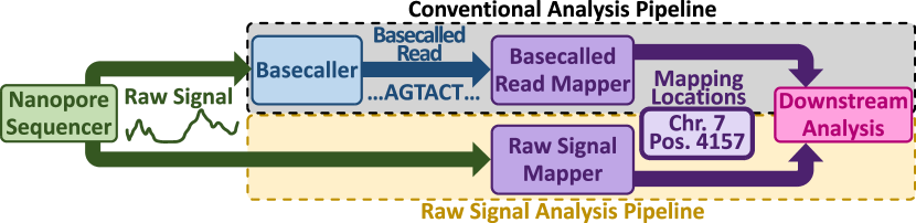
Figure 1: Conventional vs. Raw Signal Analysis Pipeline.

Real-time analysis is especially important when sequencers offer features like Oxford Nanopore Technologies’ Read Until, which allows ejecting a molecule from the pore during sequencing if it is determined to be irrelevant (e.g., by computational methods) [25]. Leveraging Read Until requires decisions to be made timely (otherwise, sequencing time is wasted) and accurately (otherwise, relevant data may be lost, or data may be biased). A timely decision requires computational analysis with throughput matching at least the sequencer, with as low latency as possible, and with as little information as possible (i.e., needing few bases to be sequenced until a decision can be reached) [24, 26]. An accurate decision may mean high sensitivity (i.e., reliably keeping relevant data), high precision (i.e., reliably rejecting irrelevant data), or a combination of both, depending on the use case.

To address the need for real-time analysis, a number of recent works propose methods for saw signal analysis without the need for basecalling (see Fig. 1, raw signal analysis pipeline). These works are based on (1) indexing methods such as k-d trees [27], FM-indices [28], or sketching with hashtables [26], (2) sequence comparison methods such as dynamic time warping [24, 29, 30, 31, 32], or (3) direct classification of raw signals using deep neural networks [33, 34, 35] or support vector machines [36].

We observe that, for small reference databases (e.g., viral genomes), these proposals for raw signal analysis typically do well in all metrics of interest (i.e., accuracy, latency, throughput, memory usage, and number of bases sequenced). However, they all fail to scale to large reference databases (e.g., the human genome) in at least one of five aspects: (1) Low accuracy, (2) low throughput, (3) high latency, (4) high memory usage, or (5) needing to sequence many bases to confidently analyze a read.

Our goal is to analyze raw nanopore signals for a wide range of reference database sizes with high accuracy, high throughput, low latency, low memory usage, and needing few bases to be sequenced. To this end, we propose RawAlign, the first nanopore raw signal mapper to follow the Seed-Filter-Align paradigm. RawAlign is inspired by traditional basecalled read mappers, such as minimap2 [37], that operate in three steps: First, during seeding, the mapper finds a large number of possible candidate locations via small exact or fuzzy matches between the read and the reference. Second, during filtering, the mapper reduces the number of seeds by heuristically evaluating and removing those that do not look promising. Third, during alignment or extension, the mapper re-evaluates all candidate locations in detail using a dynamic programming algorithm (e.g., Needleman-Wunsch [38] for basecalled data or dynamic time warping (DTW) [39, 40, 41] for raw signals).

The challenges in efficiently combining DTW with raw nanopore signal seeding and filtering approaches are two-fold. First, prior works that apply DTW to raw signal analysis without seeding and filtering (e.g., [24, 30, 29]) observe that DTW is relatively computationally expensive for small and prohibitively expensive for large reference databases. Second, we observe that existing raw signal seeding approaches generate a much larger number of candidate locations for each read than basecalled seeding approaches, meaning the DTW subroutine for evaluating each candidate location has to be called frequently. For example, for our human dataset (see §3.1.3), we observe that RawHash’s raw signal seeding approach [26] generates 10’646 candidate locations per read base on average, while minimap2’s basecalled seeding approach [37] generates only 5.12 locations per base on average. RawAlign efficiently integrates DTW with raw signal seeding by tackling these challenges from four angles:

• The number of candidate locations is reduced with RawHash’s chaining-based filtering (see §2.3)

• The number of calls to the DTW subroutine is further reduced via an early termination strategy (see §2.6.1)

• The number of arithmetic operations for the DTW computation is reduced via anchor-guided alignment (see §2.6.2) and banding/windowing (see §2.6.3)

• The arithmetic operations are implemented efficiently through SIMD vectorization (see §2.6.4)

In combination, this strategy makes DTW efficient and scalable to large genomes, enabling RawAlign to analyze raw nanopore signals efficiently and accurately for a wide range of reference database sizes.

We make the following contributions in this paper:

• We develop optimization techniques that collectively make practical the Seed-Filter-Align paradigm with dynamic time warping for raw nanopore signal analysis.

• We develop RawAlign, the first tool for raw signal mapping based on the Seed-Filter-Align paradigm.

• We comprehensively evaluate RawAlign and demonstrate its applicability to a wide range of datasets. RawAlign provides similar throughput to the prior overall state-of-the-art RawHash while improving accuracy on all datasets.

• We demonstrate that RawAlign is the first tool to map raw nanopore signals to large reference databases with high accuracy.

• We open-source all code of RawAlign and associated evaluation methodology, available at https://github.com/cmu-safari/RawAlign. RawAlign can be readily used as a raw nanopore signal mapper.

2 Materials and Methods

RawAlign works in three major steps: (1) offline reference database pre-processing (see §2.1), (2) online read pre-processing (see §2.2), and (3) online mapping of the reads with the Seed-Filter-Align paradigm (see §2.3). RawAlign uses the seeding and filtering methods from the prior work RawHash [26]. We explain the alignment based on dynamic time warping (DTW) in detail in §2.4, and we explain how RawAlign uses the result from DTW for making mapping decisions in §2.5. To make the Seed-Filter-Align paradigm practical for raw signal mapping, we introduce four strategies to improve the performance of the alignment step in §2.6.

2.1 Offline Reference Database Pre-Processing

A reference database is a set of a priori known biological sequences that reads should be compared to during mapping. For example, the reference database could consist of a chromosome, a set of genes, a genome, or multiple genomes. Reference databases are often available and accepted by read mappers in FASTA file format, i.e., as a set of basecalled nucleotide sequences. RawAlign pre-processes the reference database in two steps: First, basecalled nucleotide reference sequences are converted into a form that is easier to compare with a raw signal read (§2.1.1). Second, the reference sequences are indexed into a hash table that allows querying for small exact matches during mapping (§2.1.2).

2.1.1 Expected Event Generation

To ease comparison with a raw signal read, RawAlign converts the basecalled reference database into sequences of raw signals that would be observed in a perfect noise-free sequencer, called expected event sequences. RawAlign obtains expected event sequences in an offline pre-processing step based on a model of the nanopore provided by the manufacturer, like in prior works (e.g., [26, 27]).

2.1.2 Indexing

Mapping with the Seed-Filter-Align paradigm requires an index, a data structure that can be efficiently queried for locations of small exact matches between the read and the reference. To this end, RawAlign cuts the expected event sequences into short snippets and quantizes them into seeds. The seeds are inserted into a hash table, where each seed is a key, and the value is a list of locations where thet seed occurs in the reference database. RawAlign leverages the pre-processing steps from RawHash [26].

2.2 Online Read Pre-Processing

Current nanopore sequencers take multiple measurements as each nucleotide base passes through the nanopore, leading to many largely redundant measurements. To simplify the further computation, RawAlign converts them into event sequences, where redundant measurements are averaged into a single value. This conversion is called segmentation. It is not trivial since the translocation rate of the sequence molecule through the nanopore is variable, i.e., it is not obvious which groups of signals should be averaged together. RawAlign leverages the segmentation logic proposed in Scrappie [42] and used by Uncalled [28], Sigmap [27], and RawHash [26].

2.3 Mapping via Seed-Filter-Align

RawAlign follows the Seed-Filter-Align or Seed-Filter-Extend paradigm, inspired by conventional basecalled read mappers such as minimap2 [37]. The main mapping process consists of three steps: seeding, filtering, and alignment. Fig. 2 shows a real example of each of these steps in RawAlign for a read in the d2 E.coli dataset.

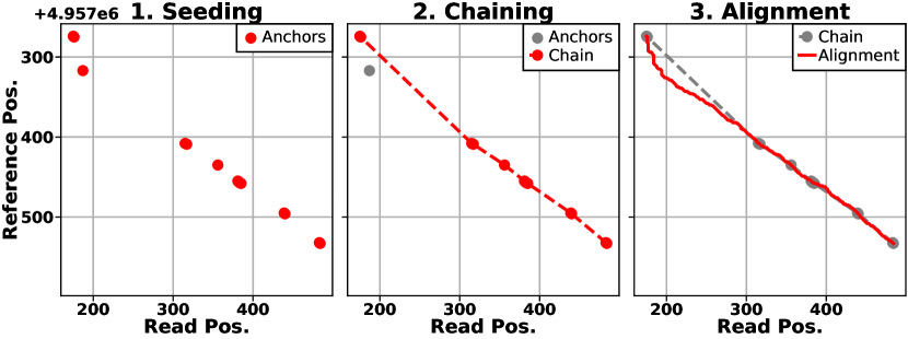
Figure 2: Example of RawAlign’s Usage of Seed-Filter-Align

2.3.1 Seeding

First, during seeding, RawAlign finds a large number of possible candidate locations via fuzzy matches between the read and the reference database (Fig. 2, left). RawAlign leverages the seeding step of RawHash [26], which works in two steps. First, it quantizes short subsequences from the read’s event sequence into seeds. Second, the locations where each seed occurs in the reference database are obtained by querying the index with the seed. The read-reference location pairs are called anchors.

2.3.2 Filtering

Second, during filtering, the mapper reduces the number of anchors by heuristically evaluating and removing those that do not look promising. One class of filters is chaining (Fig. 2, middle). During chaining, the relative positions of anchors are evaluated with a dynamic programming algorithm to identify a set of anchors that is approximately colinear in the read and reference sequence. RawAlign uses the same chaining logic as RawHash [26] and Sigmap [27].

2.3.3 Alignment

Third, during alignment or extension, RawAlign re-evaluates all remaining candidate regions at fine granularity using dynamic time warping (DTW) (Fig. 2, right). We elaborate in §2.4 why DTW [39, 40, 41, 24, 30, 29] is a natural choice to evaluate candidate locations, what its challenges are, and how RawAlign overcomes them.

2.4 Alignment via Dynamic Time Warping

Dynamic time warping (DTW) is an algorithm for fine-grained pairwise comparison and alignment of time series data [39, 40, 41], such as two raw nanopore signals. Multiple prior works use DTW to compare raw nanopore signals to entire reference genomes (e.g., SquiggleFilter [24], DTWax [30], and HARU [29]).

DTW is similar to the common Needleman-Wunsch (NW) algorithm [38], which is widely used for pairwise comparison and alignment of basecalled sequences. As shown in Fig. 3, both NW and DTW are based on dynamic programming, filling a two-dimensional table of numbers. Each entry in the dynamic programming table is computed based on three neighbor entries in the north, northwest, and west according to simple update rules. The final alignment score (for NW) or cost (for DTW) is the entry in the southwest corner of the table.

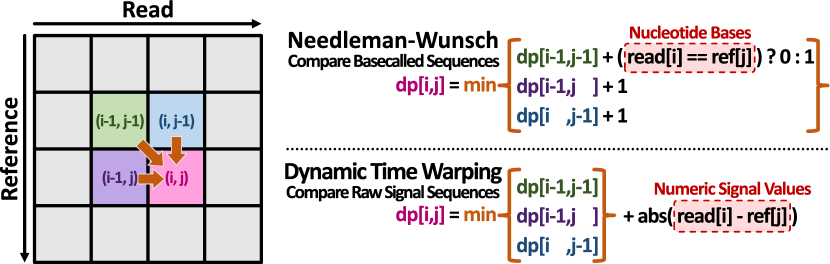
Figure 3: Conceptual Similarity of Needleman-Wunsch and Dynamic Time Warping

There are two key differences between NW and DTW: First, NW’s update rule exactly compares a read and a reference value, which is suitable for aligning basecalled sequences, where nucleotide characters either match exactly or mismatch entirely (e.g., A$=$A, A$\neq$G). In contrast, DTW compares a read and a reference value in a numeric manner, taking the absolute difference between the two. This is suitable for aligning raw signal sequences, where individual signals can match to a higher or lower degree, and exact matches are rare due to noise (e.g., 0.2$\approx$0.3, 0.1$\neq$0.9). Second, NW explicitly penalizes insertions and deletions (updates from the north and west, aka indels), independent of whether the read and reference entries match. This is suitable for aligning pairs of highly accurate basecalled sequences where insertions and deletions are relatively rare. In contrast, DTW penalizes indels according to the similarity of the read and reference values. This is suitable for aligning raw nanopore signals, where indels are expected frequently due to variable translocation rates and imperfect segmentation (see §2.2) and thus don’t necessarily indicate a poor match between the signal pair.

2.5 Alignment Score and Mapping Decisions

RawAlign bases its mapping decisions mainly on the alignment (DTW) cost (see §2.4). The DTW cost is always positive, where a low cost indicates a good match between the read and the reference, thus low-cost candidate regions should generally be preferred. However, the DTW cost monotonically increases with sequence length, meaning that a long, well-matching candidate region typically has a higher DTW cost than a short, well-matching candidate region. That is undesirable because a long, well-matching region intuitively should be preferred over a short one, as they indicate a better match between the read and the reference.

To address this issue, RawAlign employs a customized alignment scoring scheme based on the DTW cost $C_{DTW}$ and a constant match bonus $B_{Match}$ that is scaled by the number of aligned read events $N_{Read}$:

$$Score=B_{Match}\times N_{Read}-C_{DTW}$$

With this scoring scheme, longer well-matching candidate regions achieve higher scores than shorter ones, provided $B_{Match}$ is chosen appropriately. $B_{Match}$ should be chosen such that it is above the noise floor of the sequencer, i.e., such that two correctly aligned events usually differ by less than $B_{Match}$, or can be chosen using a parameter sweep.

Based on the alignment score, RawAlign considers the highest scoring candidate location as mapped if its score is at least above some threshold $Score_{Threshold}$. $Score_{Threshold}$ is necessary to avoid false positives in the presence of the match bonus; thus, the two parameters need to be chosen in conjunction.

Based on a two-dimensional parameter sweep on the d2 E.coli dataset, we choose the default parameters $B_{Match}=0.4$ and $Score_{Threshold}=20$ for all experiments and as the default for RawAlign for the best accuracy. We further discuss $B_{Match}$ in §3.5.

2.6 Performance Optimizations to DTW

We observe, like prior work (e.g., [24, 30, 29]), that DTW can have a high computational overhead if not applied judiciously. Prior works partially solve this challenge by proposing hardware accelerators for DTW [24, 30, 29]. RawAlign is, in principle, compatible with such accelerators and can benefit from them. However, to make it as out-of-the-box usable as possible, we choose to optimize the DTW in RawAlign as much as possible at the algorithm and software level. Since RawAlign’s mapping decisions require only the alignment score but not the exact alignment path, the exact path is not computed by default but can be added to the output file via a command line flag. We optimize our traceback-free DTW implementation via a combination of four techniques: (1) Early termination, (2) anchor-guided alignment, (3) banded alignment, and (4) SIMD.

2.6.1 Early Termination

Like other raw signal mappers, RawAlign outputs at most one mapping location per read. We observe that this can be exploited to terminate DTW early if it becomes clear that the current candidate location can no longer surpass the alignment score of the best already analyzed candidate location, even if the remaining (not yet aligned parts of the candidate location) were to align perfectly. This technique is most powerful if, by chance, the best candidate location with a very high alignment score is analyzed first, meaning all further alignments can be terminated more aggressively. To maximize the likelihood of the best candidate location being analyzed first, RawAlign sorts candidate locations by their chaining score before alignment.

2.6.2 Anchor-Guided Alignment

We observe that the optimal alignment of a chain typically includes the anchors in the chain. Thus, it is sufficient to align only the gaps between anchors and then combine the individual alignments or scores. Similar techniques have been applied by conventional basecalled read mappers (e.g., minimap2 [37]) and can significantly reduce the number of dynamic programming cells that need to be computed. There can be a risk of inaccurate alignments if some of the anchors are not part of the globally optimal alignment; hence, RawAlign provides command line options for either anchor-guided or global (i.e., non-anchor-guided) alignment. We observe that the accuracy loss due to anchor-guided alignment is typically small ($<1\%$ F-1 score on all evaluated datasets). Thus, RawAlign uses anchor-guided alignment by default.

2.6.3 Banded Alignment

We observe that the optimal alignment of a chain or the gap between two anchors typically follows approximately the main diagonal (see Fig. 2 for an example). This can be exploited by only computing a subset of the DTW dynamic programming table, called a band. Similar techniques have been applied by conventional basecalled read mappers and basecalled sequence aligners (e.g., Edlib [43], KSW2 [44], minimap2 [37]). Banding can significantly reduce the number of arithmetic operations and memory accesses.

We observe that the read and reference sections of candidate pairs are rarely of the same length. Hence, our banding implementation does not follow a perfect diagonal of slope 1, but rather the slope $\frac{read\_segment\_length}{reference\_segment\_length}$.

2.6.4 SIMD

DTW is a standard two-dimensional dynamic programming algorithm that can be accelerated with techniques such as SIMD, GPUs [30], FPGAs [29], or ASICs [24].

We implement our banded dynamic time warping algorithm in an antidiagonal-wise [45] fashion. We further massage the code such that GCC v11.3.0 is able to auto-vectorize the critical innermost loop of the dynamic programming computation, which we verify via compilation logs.

3 Results

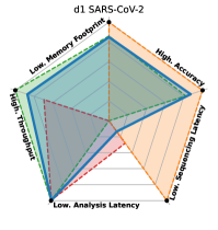
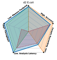
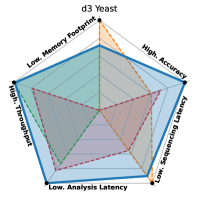
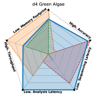
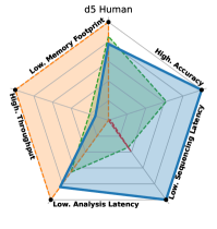
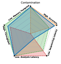
Figure 4: Accuracy-Latency-Throughput-Memory Footprint Tradeoffs of Rawalign vs. Baselines

3.1 Evaluation Methodology

3.1.1 Baselines

We demonstrate the benefits of RawAlign by comparing to three prior works: Uncalled [28], Sigmap [27], and RawHash [26]. RawAlign and all three baselines are CPU-based. They accept a set of raw signal reads (e.g., FAST5 files) and a reference database (e.g., a FASTA file) to map to, and produce mapping locations as a PAF file. We consider the mapping locations generated by minimap2 [37] as the ground truth in the read mapping experiments. In the relative abundance estimation evaluation, the ground truth is known since the read set is artificially composed of reads from multiple species; thus, we compare the accuracy of the estimates to both minimap2 and the raw signal baselines.

3.1.2 Metrics

We evaluate each tool using five categories of metrics:

• Memory footprint (GB) during mapping as reported by Ubuntu’s time package; lower is better. We also report the indexing memory footprint in Sup.Tab. 1.

• Mean throughput (bp/s) per thread of mapping as reported by each tool in its PAF output. The throughput should match at least the throughput of a nanopore (e.g., 450 bp/s in recent ONT sequencers); higher is better. We also report the median throughput in Sup.Tab. 1.

• Mean analysis latency (ms), i.e., the time spent computing for mapping reads as reported by each tool in its PAF output; lower is better. We also report the median analysis latency in Sup.Tab. 1.

• Mean sequencing latency (chunks), i.e., the number of 450 basepair-sized chunks needed to reach a mapping decision for each read, as reported by each tool in its PAF output; lower is better. Uncalled reports a number of bases instead of a number of chunks, which we convert to a number of chunks by dividing by 450. Where available, we report the sequencing latency as a number of bases in Sup.Tab. 1.

• Accuracy (F-1 score) based on the annotations from Uncalled’s pafstats tool, with minimap2’s mapping locations as the ground truth; higher is better. The F-1 score is a common way of combining precision and recall into a single metric, which we report individually in Sup.Tab. 1.

3.1.3 Datasets

We use the same datasets as RawHash’s evaluation. We updated the Green Algae dataset to use all of the available 1.3Gbp of ERR3237140, while RawHash used 0.6Gbp of ERR3237140. Tab. 1 shows the details of each dataset.

Table 1: Dataset Details

	Organism	Flow Cell	Reads	Bases	SRA	Reference	Genome
		Version	(#)	(#)	Accession	Genome	Size
Read Mapping
d1	SARS-CoV-2	R9.4	1,382,016	594M	CADDE Centre	GCF_009858895.2	29,903
d2	E. coli	R9.4	353,317	2,364M	ERR9127551	GCA_000007445.1	5M
d3	Yeast	R9.4	49,992	380M	SRR8648503	GCA_000146045.2	12M
d4	Green Algae	R9.4	63,215	1,335M	ERR3237140	GCF_000002595.2	111M
d5	Human HG001	R9.4	269,507	1,584M	FAB42260 Nanopore WGS	T2T-CHM13 (v2)	3,117M
Relative Abundance Estimation
D1-D5			2,118,047	6,257M	d1-d5	d1-d5	3,246M
Contamination Analysis
D1 and D5			1,651,523	2,178M	d1 and d5	d1	29,903
Dataset numbers (e.g., d1-d5) show the combined datasets.
Datasets are from R9.4. Base counts in millions (M).

3.1.4 System Specifications

With two exceptions, we run all CPU evaluations 64 threads on a dual-socket Intel Xeon Gold 6226R (2$\times$ 16 physical cores, 2$\times$ 32 logical cores) at 2.9GHz with 256GB of DDR4 RAM. Sigmap runs out of memory on the Intel system for the Human and Relative Abundance datasets, hence we run Sigmap with these datasets using 64 threads on a dual-socket AMD EPYC 7742 (2$\times$ 64 physical cores, 2$\times$ 128 logical cores) at 2.25GHz with 1024GB of DDR4 RAM.

3.2 Read Mapping

We run a read mapping experiment for all tools and datasets. Tab. 2 shows the raw numeric results for five key metrics: memory footprint, throughput, analysis latency, sequencing latency, and accuracy, with the best tool in each dataset and metric highlighted in bold. Fig. 4 shows the same results as a spider chart for each dataset, with each metric in a dataset normalized from worst (center, e.g., lowest throughput) to best (outside, e.g., highest throughput). Thus, a tool with a large area in the spider chart indicates a good overall tradeoff in all metrics, while a small area indicates a bad overall tradeoff between the metrics.

We make five key observations: First, RawAlign is consistently highly accurate for all datasets, and it is the only tool that is highly accurate for large reference databases (e.g., Human, Relative Abundance). Second, RawAlign has a low analysis latency (i.e., time taken for computation) and sequencing latency (i.e., time taken for sequencing). Third, RawAlign has a large area in Fig. 4 for all datasets, i.e., RawAlign generalizes well to all evaluated datasets. Fourth, RawAlign’s memory footprint depends mainly on the reference database size, requiring up to 83GB for the largest reference database (relative abundance), a size typically available in moderately sized servers. For the evaluated datasets with relatively small reference databases (d1-d4, Contamination), the memory footprint is at most 12.2GB, a size typically available in modern desktop computers and some laptops. Fifth, RawAlign’s mean throughput per thread is at least that of recent ONT nanopores (450 bp/s), i.e., a single thread can analyze the signals generated by a nanopore in real-time.

We conclude that RawAlign is the only tool to generalize well across a wide range of reference database sizes and read set compositions. It is consistently highly accurate, has low latency, meets the real-time analysis throughput requirement of 450bp/s, and fits in the memory of typical laptop, desktop, or moderately sized server systems, depending on the reference database size.

Table 2: Numeric Results

	Memory	Throughput	Analysis	Sequencing	Accuracy
d1 SARS-CoV-2	Footprint (GB)	(bp/s)	Latency (ms)	Latency (Chunks)	(F-1)
Uncalled	0.280	6,575.310	29.244	0.410	0.972
Sigmap	28.250	350,565.180	1.111	1.005	0.711
RawHash	4.210	502,043.190	0.942	1.238	0.925
RawAlign	4.520	438,089.990	1.070	1.126	0.939
d2 E.coli
Uncalled	0.800	5,174.050	115.787	1.290	0.973
Sigmap	111.170	19,215.930	34.441	2.111	0.967
RawHash	4.270	49,559.740	19.754	3.200	0.928
RawAlign	0.000	53,693.170	13.323	1.995	0.968
d3 Yeast
Uncalled	0.580	5,151.670	159.304	2.773	0.941
Sigmap	14.710	15,217.010	67.602	4.139	0.947
RawHash	4.530	17,996.930	77.586	5.826	0.906
RawAlign	4.530	17,854.670	48.394	3.071	0.963
d4 Green Algae
Uncalled	1.260	8,174.320	440.815	11.790	0.840
Sigmap	53.710	2,251.370	608.898	5.804	0.938
RawHash	14.060	5,429.580	700.304	10.646	0.824
RawAlign	12.200	5,871.450	276.094	4.514	0.932
d5 Human
Uncalled	13.170	5,612.920	1,077.536	12.959	0.320
Sigmap	313.400	195.180	16,296.435	10.401	0.327
RawHash	56.940	1,298.520	6,318.984	10.695	0.557
RawAlign	80.350	956.310	3,510.682	6.321	0.703
Contamination
Uncalled	1.060	6,607.850	199.283	3.557	0.964
Sigmap	111.650	405,956.490	1.206	2.062	0.650
RawHash	4.280	524,042.570	1.139	2.409	0.872
RawAlign	4.500	455,376.380	2.004	3.227	0.938
Relative Abundance
Uncalled	10.870	6,721.770	309.079	4.921	0.218
Sigmap	506.340	181.880	5,670.365	3.338	0.406
RawHash	60.760	596.740	2,264.014	3.816	0.459
RawAlign	83.760	480.050	1,652.162	2.336	0.754

3.3 Relative Abundance

We calculate relative abundance estimates based on the number of reads per organism reported by each tool. The read set is artificially composed of the read sets from d1-d5; hence, the ground truth is known. We consider minimap2 with basecalled reads as input as an additional baseline. We use the Euclidean distance to the ground truth relative abundance as the main accuracy metric. Tab. 3 shows the results. We report the relative abundance results based on the number of bases instead of the number of reads in Sup.§2.

We make two key observations. First, RawAlign is the most accurate among the raw signal analysis tools with a Euclidean distance of 0.12 to the ground truth and close to minimap2’s accuracy with a Euclidean distance of 0.05 to the ground truth. Second, RawAlign is the most accurate among the raw signal analysis tools for all organisms and is within 0.07 of the Euclidean distance of minimap2. Note that minimap2 has the advantage of having full-length basecalled reads as input, while RawAlign uses only a short prefix of each read for mapping.

We conclude that RawAlign can be directly used to estimate relative abundances as an end-to-end use case with high accuracy and without the need for basecalling.

Table 3: Read Ratio Relative Abundances

Tool	SARS-CoV-2	E.coli	Yeast	Green Algae	Human	Distance
Ground Truth	0.652	0.167	0.024	0.030	0.127	-
minimap2	0.613	0.163	0.025	0.053	0.147	0.050
Uncalled	0.072	0.466	0.001	0.150	0.312	0.689
Sigmap	0.201	0.446	0.002	0.123	0.229	0.549
RawHash	0.309	0.440	0.000	0.073	0.178	0.445
RawAlign	0.565	0.248	0.002	0.050	0.136	0.123

3.4 Band Width Parameter Sweep

To minimize the computational overhead of alignment, we use banded dynamic time warping (see §2.6.3). If the width of the band is chosen too narrow, accuracy will be degraded, if too wide, performance will suffer. We parameter sweep the band width as a fraction of the length of the read fragment to be aligned on the d2 E.coli dataset, and plot accuracy and throughput. Fig. 5 shows the results.

We observe that a band width of 20% of the length of the read fragment is sufficient to achieve the best accuracy (in terms of F-1 score), while simultaneously maximizing throughput. The reason that throughput is also maximized is that the pathological behavior of a too-narrow band width causes low confidence mapping candidates, meaning reads have to be analyzed for longer to reach a decision.

Based on this parameter sweep, we choose 20% as the default band width for RawAlign.

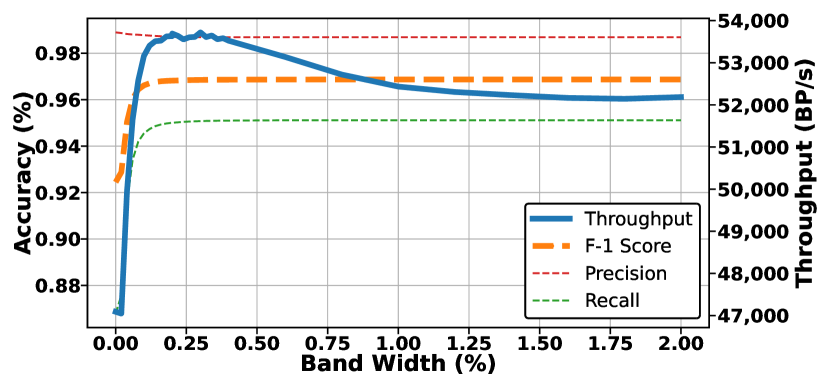
Figure 5: Band Width Parameter Sweep on d2 E.coli

3.5 Match Bonus Parameter Sweep

RawAlign makes mapping decisions based on the alignment score, which it calculates using the DTW cost and a match bonus constant scaled by the number of aligned read events (see §2.5).

We parameter sweep the match bonus parameter and measure accuracy in terms of F-1 score, precision, and recall on the d2 E.coli dataset. Fig. 6 shows the results.

We observe that an increasing match bonus improves recall, but a too-large match bonus (e.g., larger than 0.44) significantly decreases precision.

Based on this parameter sweep, we choose 0.4 as the default match bonus for RawAlign to remain on the safe side of the pathological behavior starting at a 0.44 match bonus.

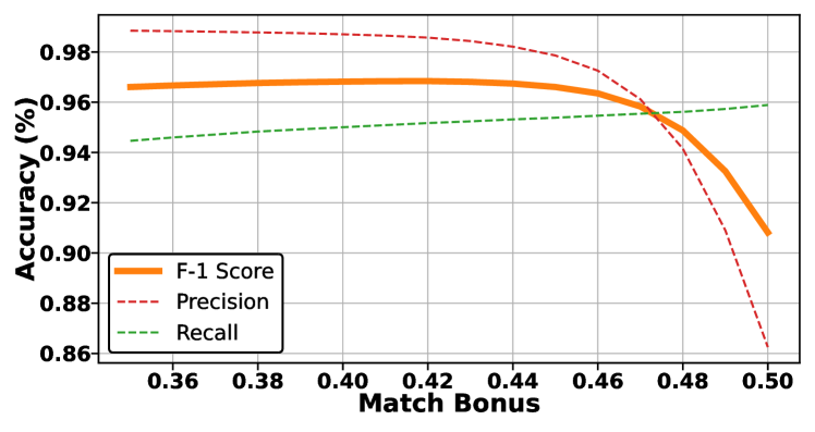
Figure 6: Match Bonus Parameter Sweep on d2 E.coli

4 Discussion and Conclusion

To our knowledge, RawAlign is the first work to combine raw signal seeding, filtering, and alignment via dynamic time warping. We have extensively compared RawAlign to Uncalled [28], Sigmap [27], and RawHash [26]. In our comparison, we have demonstrated the benefits of RawAlign’s Seed-Filter-Align approach over prior methods for raw signal mapping.

RawAlign’s Seed-Filter-Align approach is inspired by conventional basecalled read mappers. We have compared RawAlign to minimap2 in the relative abundance use case and observe that RawAlign is approaching the accuracy of minimap2. minimap2 is highly optimized and engineered, and even had full-length reads as input in that experiment; thus, it will be interesting to see how future raw signal mappers will compare to minimap2 once they are similarly optimized and engineered.

We conclude that Seed-Filter-Align is already an effective paradigm for raw signal mapping as implemented in RawAlign, and in the future may directly compete with basecalled read mappers once it is engineered to a similar extent as existing basecalled read mappers.

Funding

We acknowledge the generous gifts of our industrial partners, especially Google, Huawei, Intel, Microsoft, VMware, Xilinx. This research was partially supported by the Semiconductor Research Corporation, the ETH Future Computing Laboratory, the BioPIM project, and the Swiss National Science Foundation.

Supplementary Materials

1 Full Results

Sup.Tab. 1 reports the full results of the read mapping evaluation in §3.2 with the best tool in each dataset and metric highlighted in bold. The metrics are defined as follows:

• Indexing memory footprint (GB) during indexing as reported by Ubuntu’s time package; lower is better.

• Mapping memory footprint (GB) during mapping as reported by Ubuntu’s time package; lower is better.

• Mean throughput (bp/s) per thread of mapping as reported by each tool in its PAF output. The throughput should match at least the throughput of a nanopore (e.g., 450 bp/s in recent ONT sequencers); higher is better.

• Median throughput (bp/s) per thread of mapping as reported by each tool in its PAF output. The throughput should match at least the throughput of a nanopore (e.g., 450 bp/s in recent ONT sequencers); higher is better.

• Mean analysis latency (ms), i.e., the time spent computing for mapping reads as reported by each tool in its PAF output; lower is better. We also report the median analysis latency in Sup.Tab. 1.

• Mean sequencing latency (bases), i.e., the number of bases needed to reach a mapping decision for each read, as reported by each tool in its PAF output; lower is better.

• Mean sequencing latency (chunks), i.e., the number of 450 basepair-sized chunks needed to reach a mapping decision for each read, as reported by each tool in its PAF output; lower is better. Uncalled reports a number of bases instead of a number of chunks, which we convert to a number of chunks by dividing by 450.

• Precision based on the annotations from Uncalled’s pafstats tool, with minimap2’s mapping locations as the ground truth; higher is better.

• Recall based on the annotations from Uncalled’s pafstats tool, with minimap2’s mapping locations as the ground truth; higher is better.

• F-1 score based on the annotations from Uncalled’s pafstats tool, with minimap2’s mapping locations as the ground truth; higher is better. The F-1 score is a combination of precision and recall.

Table 1: Numeric Results

	Indexing Memory	Mapping Memory	Mean Throughput	Median Throughput	Analysis	Mean Sequencing	Mean Sequencing
d1 SARS-CoV-2	Footprint (GB)	Footprint (GB)	(bp/s)	(bp/s)	Latency (ms)	Latency (Bases)	Latency (Chunks)	Precision	Recall	F-1
Uncalled	0.070	0.280	6,575.310	6,432.800	29.244	184.509	0.410	0.955	0.991	0.972
Sigmap	0.010	28.250	350,565.180	355,001.210	1.111	-	1.005	0.993	0.554	0.711
RawHash	0.010	4.210	502,043.190	454,271.700	0.942	513.949	1.238	0.983	0.874	0.925
RawAlign	0.010	4.520	438,089.990	425,341.340	1.070	-	1.126	1.000	0.885	0.939
d2 E.coli
Uncalled	0.120	0.800	5,174.050	5,115.020	115.787	580.493	1.290	0.982	0.965	0.973
Sigmap	0.400	111.170	19,215.930	18,062.610	34.441	-	2.111	0.984	0.950	0.967
RawHash	0.350	4.270	49,559.740	44,378.530	19.754	1,375.514	3.200	0.956	0.901	0.928
RawAlign	0.390	0.000	53,693.170	47,999.640	13.323	-	1.995	0.987	0.950	0.968
d3 Yeast
Uncalled	0.300	0.580	5,151.670	4,671.330	159.304	1,247.720	2.773	0.944	0.937	0.941
Sigmap	1.040	14.710	15,217.010	14,524.360	67.602	-	4.139	0.986	0.911	0.947
RawHash	0.760	4.530	17,996.930	16,853.050	77.586	2,566.375	5.826	0.985	0.839	0.906
RawAlign	0.860	4.530	17,854.670	16,369.480	48.394	-	3.071	0.962	0.964	0.963
d4 Green Algae
Uncalled	11.960	1.260	8,174.320	8,132.010	440.815	5,305.654	11.790	0.888	0.798	0.840
Sigmap	8.630	53.710	2,251.370	2,149.510	608.898	-	5.804	0.974	0.905	0.938
RawHash	5.330	14.060	5,429.580	4,850.430	700.304	4,722.942	10.646	0.966	0.719	0.824
RawAlign	6.160	12.200	5,871.450	5,238.180	276.094	-	4.514	0.913	0.953	0.932
d5 Human
Uncalled	48.430	13.170	5,612.920	6,063.550	1,077.536	5,831.768	12.959	0.487	0.238	0.320
Sigmap	227.770	313.400	195.180	128.870	16,296.435	-	10.401	0.429	0.264	0.327
RawHash	83.090	56.940	1,298.520	268.780	6,318.984	4,772.883	10.695	0.894	0.405	0.557
RawAlign	107.440	80.350	956.310	306.390	3,510.682	-	6.321	0.698	0.708	0.703
Contamination
Uncalled	0.070	1.060	6,607.850	6,431.310	199.283	1,600.549	3.557	0.938	0.991	0.964
Sigmap	0.010	111.650	405,956.490	364,465.840	1.206	-	2.062	0.786	0.554	0.650
RawHash	0.010	4.280	524,042.570	461,280.740	1.139	1,039.429	2.409	0.870	0.874	0.872
RawAlign	0.010	4.500	455,376.380	433,378.080	2.004	-	3.227	0.997	0.885	0.938
Relative Abundance
Uncalled	47.790	10.870	6,721.770	7,232.510	309.079	2,214.647	4.921	0.763	0.127	0.218
Sigmap	238.320	506.340	181.880	165.580	5,670.365	-	3.338	0.793	0.273	0.406
RawHash	153.120	60.760	596.740	401.880	2,264.014	1,685.257	3.816	0.947	0.303	0.459
RawAlign	163.900	83.760	480.050	338.720	1,652.162	-	2.336	0.946	0.627	0.754

2 Bases Ratio Relative Abundances

We calculate relative abundance estimates based on the number of bases per organism reported by each tool. This metric corresponds to the evaluation in RawHash [26], but we believe the estimation based on the number of reads per organism is more representative in the context on ReadUntil. The read set is artificially composed of the read sets from d1-d5; hence, the ground truth is known. We consider minimap2 with basecalled reads as input as an additional baseline. We use the Euclidean distance to the ground truth relative abundance as the main accuracy metric. Sup.Tab. 2 shows the results. We report the relative abundance results based on the number of reads instead of the number of bases in §3.3.

We observe that RawAlign’s estimates are entirely inaccurate, even though it achieves a high F-1 score on the Relative Abundance dataset. The reason is that RawAlign stops sequencing each read after successfully mapping between 200-400 bases on average for all organisms (a desired property in the context of ReadUntil) thus it weights each read approximately equally. This is why the bases ratio-relative abundances reported by RawAlign are close to the read ratio-relative abundances reported in §3.3. In truth, the reads vary significantly in length, meaning RawAlign weighs them "wrongly", although it operates as desired in the context of ReadUntil. It is unclear why all raw signal baselines seemingly weigh reads correctly. Since all baselines have significantly worse F-1 scores on the Relative Abundance dataset, there is a possibility that this is down to good fortune. Note that minimap2 is run on the complete reads and not reads "cut short" due to ReadUntil, hence it can weigh the reads correctly.

We conclude that when estimating relative abundances using RawAlign, it is more representative to use the number of reads mapped instead of the number of bases mapped.

Table 2: Bases Ratio Relative Abundances

Tool	SARS-CoV-2	E.coli	Yeast	Green Algae	Human	Distance
Ground Truth	0.095	0.378	0.061	0.213	0.253	-
minimap2	0.081	0.383	0.061	0.227	0.248	0.021
Uncalled	0.002	0.561	0.000	0.228	0.208	0.219
Sigmap	0.044	0.442	0.008	0.156	0.350	0.148
RawHash	0.129	0.486	0.001	0.129	0.254	0.153
RawAlign	0.501	0.255	0.003	0.064	0.176	0.460

References

- [1] W. R. McCombie, J. D. McPherson, and E. R. Mardis, “Next-generation sequencing technologies,” Cold Spring Harbor Perspectives in Medicine, 2019.
- [2] Y. Wang, Y. Zhao, A. Bollas, Y. Wang, and K. F. Au, “Nanopore sequencing technology, bioinformatics and applications,” Nature Biotechnology, 2021.
- [3] G. A. Logsdon, M. R. Vollger, and E. E. Eichler, “Long-read human genome sequencing and its applications,” Nature Reviews Genetics, 2020.
- [4] A. M. Giani, G. R. Gallo, L. Gianfranceschi, and G. Formenti, “Long walk to genomics: History and current approaches to genome sequencing and assembly,” Computational and Structural Biotechnology Journal, 2020.
- [5] V. Boža, B. Brejová, and T. Vinař, “Deepnano: deep recurrent neural networks for base calling in minion nanopore reads,” PloS one, 2017.
- [6] Oxford Nanopore Technologies plc., “Bonito,” https://github.com/nanoporetech/bonito, 2023.
- [7] Oxford Nanopore Technologies plc., “How Basecalling Works,” https://nanoporetech.com/how-it-works/basecalling, 2023.
- [8] X. Lv, Z. Chen, Y. Lu, and Y. Yang, “An end-to-end oxford nanopore basecaller using convolution-augmented transformer,” in 2020 IEEE International Conference on Bioinformatics and Biomedicine (BIBM), 2020.
- [9] M. B. Cavlak, G. Singh, M. Alser, C. Firtina, J. Lindegger, M. Sadrosadati, N. Mansouri Ghiasi, C. Alkan, and O. Mutlu, “TargetCall: Eliminating the Wasted Computation in Basecalling via Pre-Basecalling Filtering,” APBC, 2023.
- [10] G. Singh, M. Alser, A. Khodamoradi, K. Denolf, C. Firtina, M. B. Cavlak, H. Corporaal, and O. Mutlu, “A Framework for Designing Efficient Deep Learning-Based Genomic Basecallers,” bioRxiv, 2022.
- [11] R. R. Wick, L. M. Judd, and K. E. Holt, “Performance of Neural Network Basecalling Tools for Oxford Nanopore Sequencing,” Genome Biology, 2019.
- [12] D. Neumann, A. S. Reddy, and A. Ben-Hur, “RODAN: A Fully Convolutional Architecture for Basecalling Nanopore RNA Sequencing Data,” BMC bioinformatics, 2022.
- [13] H. Konishi, R. Yamaguchi, K. Yamaguchi, Y. Furukawa, and S. Imoto, “Halcyon: an Accurate Basecaller Exploiting an Encoder-Decoder Model with Monotonic Attention,” Bioinformatics, 2021.
- [14] Z. Xu, Y. Mai, D. Liu, W. He, X. Lin, C. Xu, L. Zhang, X. Meng, J. Mafofo, W. A. Zaher et al., “Fast-bonito: A Faster Deep Learning Based Basecaller for Nanopore Sequencing,” Artificial Intelligence in the Life Sciences, 2021.
- [15] Q. Lou, S. C. Janga, and L. Jiang, “Helix: Algorithm/Architecture Co-design for Accelerating Nanopore Genome Base-calling,” in PACT, 2020.
- [16] P. Perešíni, V. Boža, B. Brejová, and T. Vinař, “Nanopore Base Calling on the Edge,” Bioinformatics, 2021.
- [17] M. Pages-Gallego and J. de Ridder, “Comprehensive and Standardized Benchmarking of Deep Learning Architectures for Basecalling Nanopore Sequencing Data,” bioRxiv, 2022.
- [18] Z. Zhang, C. Y. Park, C. L. Theesfeld, and O. G. Troyanskaya, “An Automated Framework for Efficiently Designing Deep Convolutional Neural Networks in Genomics,” Nature Machine Intelligence, 2021.
- [19] H. S. Edwards, R. Krishnakumar, A. Sinha, S. W. Bird, K. D. Patel, and M. S. Bartsch, “Real-Time Selective Sequencing with RUBRIC: Read Until with Basecall and Reference-Informed Criteria,” Scientific Reports, 2019.
- [20] A. Payne, N. Holmes, T. Clarke, R. Munro, B. J. Debebe, and M. Loose, “Readfish enables targeted nanopore sequencing of gigabase-sized genomes,” Nature Biotechnology, 2021.
- [21] M. Alser, J. Rotman, D. Deshpande, K. Taraszka, H. Shi, P. I. Baykal, H. T. Yang, V. Xue, S. Knyazev, B. D. Singer et al., “Technology dictates algorithms: recent developments in read alignment,” Genome biology, vol. 22, no. 1, p. 249, 2021.
- [22] M. Alser, J. Lindegger, C. Firtina, N. Almadhoun, H. Mao, G. Singh, J. Gomez-Luna, and O. Mutlu, “From molecules to genomic variations: Accelerating genome analysis via intelligent algorithms and architectures,” Computational and Structural Biotechnology Journal, 2022.
- [23] A. J. Mikalsen and J. Zola, “Coriolis: Enabling Metagenomic Classification on Lightweight Mobile Devices,” Bioinformatics, 2023.
- [24] T. Dunn, H. Sadasivan, J. Wadden, K. Goliya, K.-Y. Chen, D. Blaauw, R. Das, and S. Narayanasamy, “SquiggleFilter: An Accelerator for Portable Virus Detection,” MICRO, 2021.
- [25] M. Loose, S. Malla, and M. Stout, “Real-Time Selective Sequencing Using Nanopore Technology,” Nature Methods, 2016.
- [26] C. Firtina, N. M. Ghiasi, J. Lindegger, G. Singh, M. B. Cavlak, H. Mao, and O. Mutlu, “RawHash: Enabling Fast and Accurate Real-Time Analysis of Raw Nanopore Signals for Large Genomes,” ISMB/ECCB, 2023.
- [27] H. Zhang, H. Li, C. Jain, H. Cheng, K. F. Au, H. Li, and S. Aluru, “Real-time mapping of nanopore raw signals,” Bioinformatics, 2021.
- [28] S. Kovaka, Y. Fan, B. Ni, W. Timp, and M. C. Schatz, “Targeted nanopore sequencing by real-time mapping of raw electrical signal with UNCALLED,” Nature Biotechnology, 2021.
- [29] P. J. Shih, H. Saadat, S. Parameswaran, and H. Gamaarachchi, “Efficient Real-Time Selective Genome Sequencing on Resource-Constrained Devices,” GigaScience, 2023.
- [30] H. Sadasivan, D. Stiffler, A. Tirumala, J. Israeli, and S. Narayanasamy, “Accelerated Dynamic Time Warping on GPU for Selective Nanopore Sequencing,” bioRxiv, 2023.
- [31] H. Gamaarachchi, C. W. Lam, G. Jayatilaka, H. Samarakoon, J. T. Simpson, M. A. Smith, and S. Parameswaran, “GPU Accelerated Adaptive Banded Event Alignment for Rapid Comparative Nanopore Signal Analysis,” BMC Bioinformatics, vol. 21, 2020.
- [32] S. Samarasinghe, P. Premathilaka, W. Herath, H. Gamaarachchi, and R. Ragel, “Energy Efficient Adaptive Banded Event Alignment using OpenCL on FPGAs,” in ICIAfS, 2021.
- [33] Y. Bao, J. Wadden, J. R. Erb-Downward, P. Ranjan, W. Zhou, T. L. McDonald, R. E. Mills, A. P. Boyle, R. P. Dickson, D. Blaauw, and J. D. Welch, “SquiggleNet: real-time, direct classification of nanopore signals,” Genome Biology, 2021.
- [34] B. Noordijk, R. Nijland, V. J. Carrion, J. M. Raaijmakers, D. de Ridder, and C. de Lannoy, “baseLess: Lightweight Detection of Sequences in Raw MinION Data,” Bioinformatics Advances, 2023.
- [35] A. Senanayake, H. Gamaarachchi, D. Herath, and R. Ragel, “DeepSelectNet: Deep Neural Network Based Selective Sequencing for Oxford Nanopore Sequencing,” BMC Bioinformatics, 2023.
- [36] H. Sadasivan, J. Wadden, K. Goliya, P. Ranjan, R. P. Dickson, D. Blaauw, R. Das, and S. Narayanasamy, “Rapid Real-time Squiggle Classification for Read Until Using RawMap,” Arch. Clin. Biomed. Res., 2023.
- [37] H. Li, “Minimap2: pairwise alignment for nucleotide sequences,” Bioinform., vol. 34, no. 18, pp. 3094–3100, 2018. [Online]. Available: https://doi.org/10.1093/bioinformatics/bty191
- [38] S. B. Needleman and C. D. Wunsch, “A general method applicable to the search for similarities in the amino acid sequence of two proteins,” Journal of molecular biology, vol. 48, no. 3, pp. 443–453, 1970.
- [39] V. Velichko and N. Zagoruyko, “Automatic Recognition of 200 Words,” International Journal of Man-Machine Studies, 1970.
- [40] H. Sakoe and S. Chiba, “A Similarity Evaluation of Speech Patterns by Dynamic Programming,” in Nat. Meeting of Institute of Electronic Communications Engineers of Japan, 1970.
- [41] H. Sakoe and S. Chiba, “Dynamic-Programming Approach to Continuous Speech Recognition,” in Proc. International Congress of Acoustics, Budapest, 1971.
- [42] Oxford Nanopore Technologies, “Scrappie, https://github.com/nanoporetech/scrappie.”
- [43] M. Sosic and M. Sikic, “Edlib: a c/c ++ library for fast, exact sequence alignment using edit distance,” Bioinformatics, vol. 33, no. 9, pp. 1394–1395, 01 2017. [Online]. Available: https://doi.org/10.1093/bioinformatics/btw753
- [44] H. Suzuki and M. Kasahara, “Introducing Difference Recurrence Relations for Faster Semi-Global Alignment of Long Sequences,” BMC Bioinformatics, 2018.
- [45] Z. Xia, Y. Cui, A. Zhang, T. Tang, L. Peng, C. Huang, C. Yang, and X. Liao, “A review of parallel implementations for the smith–waterman algorithm,” Interdisciplinary Sciences: Computational Life Sciences, 2022.