Compressed online Sinkhorn

Abstract

The use of optimal transport (OT) distances, and in particular entropic-regularised OT distances, is an increasingly popular evaluation metric in many areas of machine learning and data science. Their use has largely been driven by the availability of efficient algorithms such as the Sinkhorn algorithm. One of the drawbacks of the Sinkhorn algorithm for large-scale data processing is that it is a two-phase method, where one first draws a large stream of data from the probability distributions, before applying the Sinkhorn algorithm to the discrete probability measures. More recently, there have been several works developing stochastic versions of Sinkhorn that directly handle continuous streams of data. In this work, we revisit the recently introduced online Sinkhorn algorithm of [Mensch and Peyré, 2020]. Our contributions are twofold: We improve the convergence analysis for the online Sinkhorn algorithm, the new rate that we obtain is faster than the previous rate under certain parameter choices. We also present numerical results to verify the sharpness of our result. Secondly, we propose the compressed online Sinkhorn algorithm which combines measure compression techniques with the online Sinkhorn algorithm. We provide numerical experiments to show practical numerical gains, as well as theoretical guarantees on the efficiency of our approach.

1 Introduction

A fundamental problem in data processing is the computation of metrics or distances to effectively compare different objects of interest [Peyré et al., 2019]. In the last decade, it has become apparent that many problems, including image processing [Ferradans et al., 2014, Ni et al., 2009], natural language processing [Xu et al., 2020] and genomics [Schiebinger et al., 2019], can be modelled using probability distributions and optimal transport (OT) or Wasserstein distances have become widely adopted as evaluation metrics. The use of such distances have become especially prevalent in the machine learning community thanks to the vast amount of research in computational aspects of entropic-regularised optimal transport [Cuturi, 2013, Peyré et al., 2019]. The use of entropic-regularised optimal transport has been especially popular since they can be easily computed using the celebrated Sinkhorn algorithm [Cuturi, 2013], and such distances are known to have superior statistical properties, circumventing the curse of dimensionality [Genevay et al., 2019].

Given the wide-spread interest in computational optimal transport and in particular, entropic regularised distances in large data-processing applications, there have been several lines of work on extending the Sinkhorn algorithm to handle large-scale datasets. The application of the Sinkhorn algorithm typically involves first drawing samples from the distributions of interest and constructing a large pairwise distance matrix, then applying the Sinkhorn algorithm to compute the distance between the sampled empirical distributions. While there have been approaches to accelerate the second step with Nyström compression [Altschuler et al., 2019] or employing greedy approaches [Altschuler et al., 2017], in recent years, there has been an increasing interest in the development of online versions of Sinkhorn that can directly compute OT distances between continuous distributions. One of the computational challenges for computing the OT distance between continuous distributions is that the dual variables (Kantorovich potentials) are continuous functions and one needs to represent these functions in a discrete manner. Two of the main representations found in the literature include the use of reproducing kernel Hilbert spaces [Aude et al., 2016] and more recently, the online Sinkhorn algorithm [Mensch and Peyré, 2020] was introduced where the Kantorovich potentials are represented using sparse measures and special kernel functions that exploit the particular structure of OT distances.

Contributions

In this work, we revisit the online Sinkhorn algorithm of [Mensch and Peyré, 2020]: we improve their theoretical convergence result for this method, and propose a compressed version of this method to alleviate the large memory footprint of this method. Our contributions can be summarised as follows

• We provide an updated theoretical convergence rate that is under certain parameter choices is faster than the rate given in [Mensch and Peyré, 2020]. We also numerically verify that our theoretical analysis is sharp.

• We propose a compressed version of the online Sinkhorn algorithm. The computational complexity of the online Sinkhorn algorithm grows polynomially with each iteration and it is natural to combine compression techniques with the online Sinkorn algorithm. As explained in Section 3, the online Sinkhorn algorithm seeks to represent the continuous Kantorovich potentials as measures (super-position of Diracs) and there are some popular methods for measure compression such as kernel recombination [Cosentino et al., 2020, Hayakawa et al., 2022, Adachi et al., 2022]) and Nyström method [Zhang et al., 2008]. We apply compression with a Fourier-based moments approach. We present theoretical complexity analysis and numerical experiments to show that our approach can offer significant computational benefits.

2 Online Sinkhorn

2.1 The Sinkhorn algorithm

Let $\mathcal{X}$ be a compact subset of $\mathbb{R}^{d}$ and $\mathcal{C}(\mathcal{X})$ denote the set of continuous functions $\mathcal{X}\to\mathbb{R}$. The Kantorovich formulation was first proposed to study the transport plan between two probability distributions $\alpha,\beta$ with the minimal cost [Kantorovich, 1942]:

$$\min_{\pi\in\Pi(\alpha,\beta)}\int C(x,y)\mathrm{d}\pi(x,y),$$ (1)

where $\Pi(\alpha,\beta)$ is the set of positive measures with fixed marginals $\alpha$ and $\beta$,

$$\Pi(\alpha,\beta)\stackrel{{\scriptstyle\mbox{\tiny def.}}}{{=}}\left\{\pi\in\mathcal{P}(\mathcal{X}^{2})\colon\alpha=\int_{y\in\mathcal{X}}\mathrm{d}\pi(\cdot,y),\;\beta=\int_{x\in\mathcal{X}}\mathrm{d}\pi(x,\cdot)\right\},$$ (2)

and $C\colon\mathcal{X}\times\mathcal{X}\to\mathbb{R}$ is a given cost function.

The solution to the optimisation problem equation 1 above can be approximated by a strictly convex optimisation problem by adding a regularisation term: The entropic regularised OT problem with the regularisation parameter $\varepsilon>0$ is

$$\underset{\pi\in\Pi(\alpha,\beta)}{\min}\int C(x,y)\mathrm{d}\pi(x,y)+\varepsilon\text{KL}\left(\pi,\alpha\otimes\beta\right),$$ (3)

where $\alpha\otimes\beta$ is the product measure on $\mathcal{X}^{2}$, and $\text{KL}\left(\pi,\alpha\otimes\beta\right)\stackrel{{\scriptstyle\mbox{\tiny def.}}}{{=}}\int\log\left(\frac{\mathrm{d}\pi}{\mathrm{d}\alpha\otimes\beta}\right)\mathrm{d}\pi$ is the Kulback–Leibler divergence [Cuturi, 2013].

The following maximisation problem for $\varepsilon>0$ is a dual formulation of the entropic regularised OT problem equation 3:

$$F_{\alpha,\beta}(f,g)\coloneqq\underset{f,g\in\mathcal{C}\left(\mathcal{X}\right)}{\max}\int f(x)d\alpha(x)+\int g(y)d\beta(y)-\varepsilon\int e^{\frac{f\oplus g-C}{\varepsilon}}d\alpha(x)d\beta(y)$$

where $\left(f\oplus g-C\right)\left(x,y\right)\coloneqq f(x)+g(y)-C(x,y)$ and $\left(f,g\right)$ are defined to be the pair of dual potentials [Peyré et al., 2019].

The Sinkhorn algorithm works by alternating minimization on the dual problem $F_{\alpha,\beta}$, and is for discrete distributions. So, to apply Sinkhorn, one first draws empirical distributions $\alpha_{n}\stackrel{{\scriptstyle\mbox{\tiny def.}}}{{=}}\frac{1}{n}\sum_{i=1}^{n}\delta_{x_{i}}$ and $\beta_{n}\stackrel{{\scriptstyle\mbox{\tiny def.}}}{{=}}\frac{1}{n}\sum_{j=1}^{n}\delta_{y_{i}}$ with $x_{i}\overset{\mathrm{iid}}{\sim}\alpha$ and $y_{i}\overset{\mathrm{iid}}{\sim}\beta$, then compute iteratively:

$$\begin{split}u_{t+1}=\left(\frac{1}{n}\sum_{j=1}^{n}\frac{1}{v_{t,j}}\exp\left(-\frac{C(x_{k},y_{j})}{\varepsilon}\right)\right)_{k=1}^{n},\quad v_{t+1}=\left(\frac{1}{n}\sum_{i=1}^{n}\frac{1}{u_{t+1,i}}\exp\left(\frac{-C\left(x_{i},y_{k}\right)}{\varepsilon}\right)\right)_{k=1}^{n},\end{split}$$ (4)

where $u_{t}\stackrel{{\scriptstyle\mbox{\tiny def.}}}{{=}}\exp\left(-f_{t}/\varepsilon\right)\in\mathbb{R}^{n}$ and $v_{t}\stackrel{{\scriptstyle\mbox{\tiny def.}}}{{=}}\exp\left(-g_{t}/\varepsilon\right)\in\mathbb{R}^{n}$ and $f_{t},g_{t}\in\mathbb{R}^{n}$ are the pair of dual potentials at step $t$. The computational complexity is $O\left(n^{2}\log\left(n\right)\delta^{-3}\right)$ for reaching $\delta$ accuracy [Altschuler et al., 2017, Mensch and Peyré, 2020].

2.2 The online Sinkhorn algorithm

In the continuous setting, the Sinkhorn iterations operate on functions $u_{t},v_{t}\in\mathcal{C}(\mathcal{X})$ and involve the full distributions $\alpha,\beta$:

$$u_{t+1}=\exp\left(-\frac{f_{t+1}}{\varepsilon}\right)=\int\frac{1}{v_{t}(y)}K_{y}(\cdot)d\beta(y),\quad v_{t+1}=\exp\left(-\frac{g_{t+1}}{\varepsilon}\right)=\int\frac{1}{u_{t+1}(x)}K_{x}(\cdot)d\alpha(x),$$ (5)

where $K_{y}(\cdot)=\exp\left(-\frac{C(\cdot,y)}{\varepsilon}\right)$ and $K_{x}(\cdot)=\exp\left(-\frac{C(x,\cdot)}{\varepsilon}\right)$. In [Mensch and Peyré, 2020], a natural extension of the Sinkhorn algorithm was proposed, replacing $\alpha$ and $\beta$ at each step with empirical distributions of growing supports $\hat{\alpha}_{t}=\frac{1}{n}\sum_{i=n_{t}}^{n_{t+1}}\delta_{x_{i}}$ and $\hat{\beta}_{t}=\frac{1}{n}\sum_{i=n_{t}+1}^{n_{t+1}}\delta_{y_{i}}$ where $x_{i}\overset{\mathrm{iid}}{\sim}\alpha$ and $y_{i}\overset{\mathrm{iid}}{\sim}\beta$. For appropriate learning rate $\eta_{t}$, the online Sinkhorn iterations are defined as

$$u_{t+1} =\left(1-\eta_{t}\right)u_{t}+\eta_{t}\int\frac{1}{v_{t}(y)}K_{y}(\cdot)\mathrm{d}\hat{\beta}_{t}(y),$$ (6)

$$v_{t+1} =\left(1-\eta_{t}\right)v_{t}+\eta_{t}\int\frac{1}{u_{t+1}(x)}K_{x}(\cdot)\mathrm{d}\hat{\alpha}_{t}(x).$$ (7)

The key observation in [Mensch and Peyré, 2020] is that the continuous functions $u_{t}$ and $v_{t}$ can be discretely represented using vectors $(q_{i,t},y_{i})$ and $(p_{i,t},x_{i})$, in particular, $u_{t}$ and $v_{t}$ take the following form:

$$u_{t}=\sum_{i=1}^{n_{t}}\exp\left(\frac{q_{i,t}-C(\cdot,y_{i})}{\varepsilon}\right)\quad\text{and}\quad v_{t}=\sum_{i=1}^{n_{t}}\exp\left(\frac{p_{i,t}-C(x_{i},\cdot)}{\varepsilon}\right),$$ (8)

where $q_{i,t},p_{i,t}$ are weights and $\left(x_{i},y_{i}\right)$ are the positions, for $1\leqslant i\leqslant n_{t}$. Thanks to this representation on $u_{t},v_{t}$, the online Sinkhorn algorithm only needs to record and update vectors $(p_{i,t},x_{i})_{i}$ and $(q_{i,t},y_{i})_{i}$. The algorithm is summarised in Algorithm 1.

Input: Distributions $\alpha$ and $\beta$, learning weights $(\eta_{t})_{t}$, batch sizes $\left(b_{t}\right)_{t}$

Set $p_{i}=q_{i}=0$ for $i\in(0,n_{0}]$, where $n_{0}=b_{0}$

for $t=0,\cdots,T-1$ do

      

1. Sample $(x_{i})_{(n_{t},n_{t+1}]}\overset{\mathrm{iid}}{\sim}\alpha$, $(y_{i})_{(n_{t},n_{t+1}]}\overset{\mathrm{iid}}{\sim}\beta$, where $n_{t+1}=n_{t}+b_{t}$

2. Evaluate $(g_{t}(y_{i}))_{i=(n_{t},n_{t+1}]}$ via equation 8

3. $q_{(n_{t},n_{t+1}],t+1}\leftarrow\varepsilon\log(\frac{\eta_{t}}{b_{t+1}})+\left(g_{t}(y_{i})\right)_{(n_{t},n_{t+1}]}$

4. $q_{(0,n_{t}],t+1}\leftarrow q_{(0,n_{t}],t}+\varepsilon\log(1-\eta_{t})$

5. Evaluate $(f_{t+1}(x_{i}))_{i=(n_{t},n_{t+1}]}$ via equation 8

6. $p_{(n_{t},n_{t+1}],t+1}\leftarrow\varepsilon\log(\frac{\eta_{t}}{b_{t+1}})+\left(f_{t+1}(x_{i})\right)_{(n_{t},n_{t+1}]}$

7. $p_{(0,n_{t}],t+1}\leftarrow p_{(0,n_{t}],t}+\varepsilon\log(1-\eta_{t})$

Returns: ${f}_{T}:(q_{i,T},y_{i})_{(0,n_{T}]}$ and ${g}_{T}:(p_{i,T},x_{i})_{(0,n_{T}]}$

Algorithm 1 Online Sinkhorn (Mensch and Peyré, 2020)

2.2.1 Convergence analysis for online Sinkhorn

Following [Mensch and Peyré, 2020], convergence can be established under the following three assumptions.

Assumption 1.

The cost $C:\mathcal{X}\times\mathcal{X}\to\mathbb{R}$ is $L$-Lipschitz continuous for some Lipschitz constant $L>0$.

Assumption 2.

$(\eta_{t})_{t}$ is such that $\sum_{t=1}^{\infty}\eta_{t}=\infty$ and $\sum_{t=1}^{\infty}\eta_{t}^{2}<\infty$, where $0<\eta_{t}<1$ for all $t>0$.

Assumption 3.

$\left(b_{t}\right)_{t}$ and $\left(\eta_{t}\right)_{t}$ satisfy that $\sum_{t=1}^{\infty}\frac{\eta_{t}}{\sqrt{b_{t}}}<\infty$.

In order to satisfy Assumptions 2 and 3, from now on, we let $-1<b<-\frac{1}{2}$ and $a-b>1$ and take

$$\eta_{t}=t^{b}\quad\text{and}\quad b_{t}=t^{2a}.$$

For the online Sinkhorn algorithm, we obtain the following convergence result:

Theorem 1.

Let $f^{*}$ and $g^{*}$ denote the optimal potentials. Let ${f}_{t}$ and ${g}_{t}$ be the output of Algorithm 1 after $t$ iterations. Suppose $\eta_{t}=t^{b}$ for $-1<b<-\frac{1}{2}$, and $b_{t}=t^{2a}$ with $a-b>1$. For a constant $c>0$,

$$\delta_{N}\lesssim\exp\left(-cN^{\frac{b+1}{2a+1}}\right)+N^{-\frac{a}{2a+1}}={O}\left(N^{-\frac{a}{2a+1}}\right),$$ (9)

where

$$\delta_{N}\stackrel{{\scriptstyle\mbox{\tiny def.}}}{{=}}\left\|\left(f_{t\left(N\right)}-f^{*}\right)/\varepsilon\right\|_{var}+\left\|\left(g_{t\left(N\right)}-g^{*}\right)/\varepsilon\right\|_{var},$$

and ${t\left(N\right)}$ is the first iteration number for which $\sum_{i=1}^{t}b_{i}>N$.

Comparison with the previous rate

It was shown in [Mensch and Peyré, 2020, Proposition 4] that

$$\delta_{N}\lesssim\exp\left(-cN^{\frac{b+1}{2a+1}}\right)+N^{\frac{b}{2a+1}}.$$

By taking $b$ close to $-1$ and $a$ close to 0, the asymptotic convergence rate can be made arbitrarily close to ${O}\left(N^{-1}\right)$. There however seems to be an error in the proof (see comment after the sketch proof and the appendix). In contrast, our asymptotic convergence rate is ${O}\left(N^{-\frac{a}{2a+1}}\right)$, which is at best ${O}(N^{-1/2})$. However, our convergence rate is faster whenever $a\geqslant-b$. See Figure 1.

Sketch of proof

Let $U_{t}\stackrel{{\scriptstyle\mbox{\tiny def.}}}{{=}}\left(f_{t}-f^{*}\right)/\varepsilon$, $V_{t}\stackrel{{\scriptstyle\mbox{\tiny def.}}}{{=}}\left(g_{t}-g^{*}\right)/\varepsilon$, $e_{t}\stackrel{{\scriptstyle\mbox{\tiny def.}}}{{=}}\|U_{t}\|_{var}+\|V_{t}\|_{var}$, $\zeta_{\hat{\beta}_{t}}\stackrel{{\scriptstyle\mbox{\tiny def.}}}{{=}}\left(T_{\beta}(g_{t})-T_{\hat{\beta}_{t}}(g_{t})\right)/\varepsilon$ and $\iota_{\hat{\alpha}_{t}}\stackrel{{\scriptstyle\mbox{\tiny def.}}}{{=}}\left(T_{\alpha}(f_{t+1})-T_{\hat{\alpha}_{t}}(f_{t+1})\right)/\varepsilon$, where $T_{\mu}$ is defined in Appendix A.2. It can be shown that

$$e_{t+1}\leqslant\left(1-\eta_{t}+\eta_{t}\kappa\right)e_{t}+\eta_{t}\left(\|\zeta_{\beta_{t}}\|_{var}+\|\iota_{\alpha_{t}}\|_{var}\right),$$

and

$$\mathbb{E}\left\|\zeta_{\hat{\beta}_{t}}\right\|_{var}\lesssim\frac{A_{1}(f^{*},g^{*},\varepsilon)}{\sqrt{b_{t}}}\quad\text{and}\quad\mathbb{E}\left\|\iota_{\hat{\alpha}_{t}}\right\|_{var}\lesssim\frac{A_{2}(f^{*},g^{*},\varepsilon)}{\sqrt{b_{t}}},$$

where $A_{1}(f^{*},g^{*},\varepsilon),A_{2}(f^{*},g^{*},\varepsilon)$ are constants depending on $f^{*},g^{*},\varepsilon$.

Denote $S=A_{1}(f^{*},g^{*},\varepsilon)+A_{2}(f^{*},g^{*},\varepsilon)$, then taking expectations

$$\mathbb{E}e_{t+1}\lesssim\left(1-\eta_{t}+\eta_{t}\kappa\right)\mathbb{E}e_{t}+\frac{S\eta_{t}}{\sqrt{b_{t}}}.$$ (10)

Applying the Gronwall lemma [Mischler, 2018, Lemma 5.1] to this recurrence relation, we get

$$\mathbb{E}e_{t+1}\lesssim\left(\mathbb{E}e_{1}+\frac{S}{a-b-1}\right)\exp\left(\frac{\kappa-1}{b+1}t^{b+1}\right)+t^{-a}.$$ (11)

The total number of samples $N=O(t^{(2a+1)})$ and this substitution completes the proof. ∎

In [Mensch and Peyré, 2020], the last term of the upper bound in equation 11 was calculated as $t^{b}$, but this followed the derivations of [Moulines and Bach, 2011, Theorem 2] that do not directly apply, which leads to the error in Theorem 1 to be $O\left(N^{\frac{b}{2a+1}}\right)$.

2.2.2 Numerical verification of our theoretical rate

To show that the error rates in Theorem 1 are correct, we plot the variational error for online Sinkhorn and display our theoretical convergence rate with exponent $\frac{-a}{2a+1}$ and the ‘old theoretical’ convergence rate with exponent ${\frac{b}{2a+1}}$ from [Mensch and Peyré, 2020, Proposition 4].

Our experiments are in $1$D, $2$D and $5$D. For the $1$D case, the source and target distributions are the Gaussian distributions $\mathcal{N}\left(3,4\right)$ and $\mathcal{N}\left(1,2\right)$. In $2$D, the source distribution $\mathcal{N}\left(\mu^{(1)},\Sigma^{(1)}\right)$ is generated by $\mu_{i}^{(1)}\sim\mathcal{U}\left(0,10\right)$, for $i=1,2$ and $\Sigma^{(1)}$ is a randomly generated covariance matrix. The target distribution $\mathcal{N}\left(\mu^{(2)},\Sigma^{(2)}\right)$ is generated by $\mu_{i}^{(2)}\sim\mathcal{U}\left(0,5\right)$, for $i=1,2$ and $\Sigma^{(2)}$ is a randomly generated covariance matrix. The $y$-axis in all the plots in this section are the errors of the potential functions $\left\|f_{t}-f_{t-1}\right\|_{var}+\left\|g_{t}-g_{t-1}\right\|_{var}$ based on a finite set of points $x_{i},y_{i}$. The plots show that the convergence behaviour of online Sinkhorn asymptotically is parallel to our theoretical line, which corroborates with Theorem 1.

​ ​

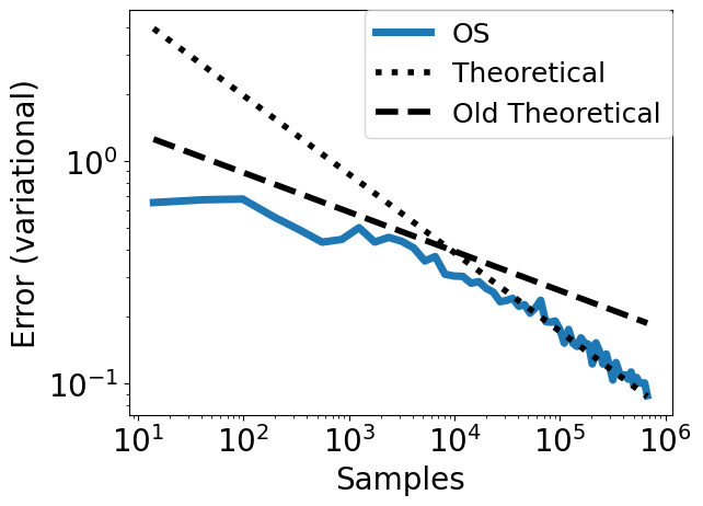
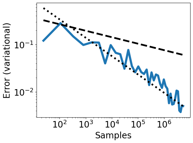
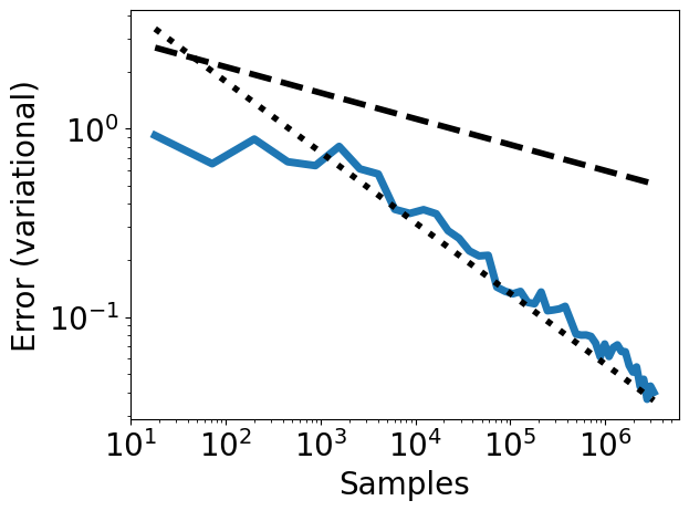
Figure 1: Left: $\varepsilon=0.3$, $a=1.2$, $b=-0.6$, $d=1$. The theoretical rate of convergence is $-0.35$ (compared to the old rate of $-0.18$); a linear fit shows OS is converging with rate $-0.31$. Middle: $\varepsilon=0.3$, $a=1.7$, $b=-0.6$, $d=2$ with rates $\texttt{Theoretical}=-0.39$; $\texttt{Old theoretical}=-0.14$ ; $\texttt{OS}=-0.37$. Right: $\varepsilon=0.4$, $a=1.5$, $b=-0.55$, $d=5$ with rates $\texttt{Theoretical}=-0.38$; $\texttt{Old theoretical}=-0.14$ ; $\texttt{OS}=-0.41$.

3 Compressed online Sinkhorn

3.1 Complexity of online Sinkhorn

The online Sinkhorn algorithm’s prolonged runtime is due to the evaluation of $(u_{t},v_{t})$ in equation 8 on an increasing amount of newly drawn data. In Algorithm 1, due to the calculation of the cost matrix $C(x_{i},y_{j})$ for ${i=(n_{t},n_{t+1}],j=(0,n_{t}]}$ in equation 8, the complexity is $O\left(n_{t}b_{t}\right)=O\left(t^{4a+2}\right)$ and the memory cost for $\left(x_{i},y_{i}\right)_{i=(0,n_{t}]}$ is $O\left(n_{t}\right)=O\left(t^{2a+1}\right)$. The complexity and memory cost increase polynomially with each iteration; therefore, the Algorithm 1 will require a computing unit with higher capacity as the iteration progresses.

3.2 Compressed online Sinkhorn

To reduce the complexity and memory costs, we propose the compressed online Sinkhorn algorithm. To explain our derivation, we focus on obtaining a compressed version of $u_{t}$; the function $v_{t}$ can be treated in a similar manner. From equation 8, we have $u_{t}(x)=\int\frac{K_{x}\left(y\right)}{\varphi\left(y\right)}\mathrm{d}\mu\left(y\right)$ for $\mu\stackrel{{\scriptstyle\mbox{\tiny def.}}}{{=}}\sum_{i=1}^{n_{t}}\exp\left(\frac{q_{i,t}}{\varepsilon}\right)\varphi\left(y_{i}\right)\delta_{y_{i}}$, $K_{x}(y)\stackrel{{\scriptstyle\mbox{\tiny def.}}}{{=}}\exp(-C(x,y)/\varepsilon)$ and any positive function $\varphi$. The idea of our compression method is to exploit measure compression techniques to replace $\mu$ with a measure $\hat{\mu}$ made up of $m\ll n_{t}$ Diracs. We then approximate $u_{t}$ with $\hat{u}_{t}(x)=\int\frac{K_{x}\left(y\right)}{\varphi\left(y\right)}\mathrm{d}\hat{\mu}(y)$. Let $\varphi=v_{t}=\exp\left(-\frac{g_{t}}{\varepsilon}\right)$, then $\exp\left(\frac{q_{i,t}}{\varepsilon}\right)\varphi\left(y_{i}\right)\leq 1$ by the update 3 Algorithm 1. The weights for $\mu$ are hence bounded and it is easier to compress $\mu$.

To ensure that $\hat{u}_{t}\approx u_{t}$, we will enforce that the measure $\hat{\mu}$ satisfies

$$\int P_{k}\left(y\right)\mathrm{d}\mu\left(y\right)=\int P_{k}\left(y\right)\mathrm{d}\hat{\mu}\left(y\right)$$ (12)

for some appropriate set of functions $\left\{P_{k}\;;\;k\in\Omega\right\}$, where $\Omega$ is some set of cardinality $m_{t}$. Let us introduce a couple of ways to choose such functions.

Example: Gaussian quadrature

In dimension 1 (covered here mostly for pedagogical purposes), one can consider the set of polynomials up to degree $2m-1$, denoted by $\mathbb{P}_{2m-1}$ for some $m\in\mathbb{N}$. For well-ordered $y_{i}$, the constraints (12) defines the $m$-point Gaussian quadrature $\hat{\mu}=\sum\hat{w}_{i}\delta_{\hat{y}_{i}}$, and both new weights $\hat{w}_{i}$ and new nodes $\hat{y}_{i}$ are required to achieve this. Numerically, this can be efficiently implemented following the OPQ Matlab package [Gautschi, 2004] and the total complexity for the compression is $O\left(m^{3}+n_{t}m\right)$. To define $\hat{u}_{t}$, solve $e^{\hat{q}_{i,t}/\varepsilon}v_{t}(\hat{y}_{i})=\hat{w}_{i}$ for $\hat{q}_{i,t}$ and let $\hat{u}_{t}(x)=\sum_{i=1}^{m}\exp(\hat{q}_{i,t}/\varepsilon)K_{x}(\hat{y}_{i})$.

Example: Fourier moments

Since we expect that the compressed function $\hat{u}_{t}$ satisfies $\hat{u}_{t}\approx u_{t}$, one approach is to ensure that the Fourier moments of $\hat{u}_{t}$ and $u_{t}$ match on some set of frequencies. Observe that the Fourier transform of $u_{t}(x)=\int\frac{K_{x}}{v_{t}}\left(y\right)\mathrm{d}\mu(y)$ can be written as

$$\int\exp\left(-ikx\right)\int\frac{K_{x}}{v_{t}}\left(y\right)\mathrm{d}\mu\left(y\right)\mathrm{d}x=\int\frac{\hat{K}_{y}(k)}{v_{t}(y)}\mathrm{d}\mu\left(y\right),\quad\text{where}\quad\hat{K}_{y}(k)\stackrel{{\scriptstyle\mbox{\tiny def.}}}{{=}}\int K_{x}(y)\exp\left(-ikx\right)\mathrm{d}x.$$ (13)

We therefore let $P_{k}(y)=\frac{\hat{K}_{y}(k)}{v_{t}\left(y\right)}$ in equation 12, for suitably chosen frequencies $k$ (see Appendix A.5.2).

In contrast to GQ, we retain the current nodes $y_{i}$ and seek new weights $\hat{w}_{i}$ such that $\hat{\mu}=\sum_{i=1}^{m}\hat{w}_{i}\delta_{y_{i}}$ satisfies $\int\frac{\hat{K}_{y}(k)}{v_{t}(y)}\mathrm{d}\left(\mu-\hat{\mu}\right)\left(y\right)=0$. Let $b_{t}=\left(\int P_{k}(y)d\mu(y)\right)$ and $M_{t}=\left(P_{k}(y_{i})\right)_{k\in\Omega,i\in[n_{t}]}$; equivalently, we seek $\hat{w}\geq 0$ such that $M_{t}\hat{w}=b_{t}$. We know from the Caratheodory theorem that there exists a solution with only $m+1$ positive entries in $\hat{w}$, and the resulting compressed measure $\hat{\mu}=\sum_{\hat{w}_{i}>0}\hat{w}_{i}\delta_{\hat{y}_{i}}$. Algorithms to find the Caratheodory solution include [Hayakawa et al., 2022] and [Tchernychova, 2015]. We may also find $\hat{w}\geq 0$ to minimise $\|M_{t}\hat{w}-b_{t}\|^{2}$ using algorithms such as [Virtanen et al., 2020] and [Pedregosa et al., 2011], which in practice is faster but leads to a sub-optimal support: in our experiments, these methods contain up to $10m$ points. Theoretically, as long as the size of the support is $O(m)$, the same behaviour convergence guarantees hold, so although the non-negative least squares solvers do not provide this guarantee, we find it to be efficient and simple to implement in practice. The complexity of calculating the matrix $M_{t}$ is $O\left(dmn_{t}\right)$, and for solving the linear system is $O\left(m^{3}\right)$ or $O\left(m^{3}\log n_{t}\right)$ depending on the solution method. Therefore, the total complexity for the compression method is $O\left(m^{3}+dmn_{t}\right)$ or $O\left(m^{3}\log n+dmn_{t}\right)$. In practice, we found the non-negative least squares solvers to be faster and to give good accuracy. The compressed online Sinkhorn algorithm is summarised in Algorithm 2. The main difference is the Steps 8 and 9, where the further compression steps are taken after the online Sinkhorn updates in Algorithm 1. This reduces the complexity of the evaluation of $(f_{t},g_{t})$ in the next iteration.

Input: Distributions $\alpha$ and $\beta$, learning rates $\left(\eta_{t}\right)_{t}=\left(\left(t+1\right)^{b}\right)_{t}$, batch size $\left(b_{t}\right)_{t}=\left(\left(t+1\right)^{2a}\right)_{t}$, such that $-1<b<-\frac{1}{2}$ and $a-b>1$

Initialisation: $n_{1}=m_{1}=b_{1},\hat{p}_{i,1}=\hat{q}_{i,1}=0$, $\hat{x}_{i,1}\overset{\mathrm{iid}}{\sim}\alpha,\hat{y}_{i,1}\overset{\mathrm{iid}}{\sim}\beta$ for $i\in(0,m_{1}]$

for $t=1,\cdots,T-1$ do

      

1. Sample $(x_{i})_{(n_{t},n_{t+1}]}\overset{\mathrm{iid}}{\sim}\alpha$, $(y_{i})_{(n_{t},n_{t+1}]}\overset{\mathrm{iid}}{\sim}\beta$, where $n_{t+1}=n_{t}+b_{t}$. Let $\left(\hat{x}_{i,t}\right)_{(m_{t},m_{t}+b_{t}]}=(x_{i})_{(n_{t},n_{t+1}]}$, $\left(\hat{y}_{i,t}\right)_{(m_{t},m_{t}+b_{t}]}=(y_{i})_{(n_{t},n_{t+1}]}$.

2. Evaluate $(\hat{g}_{t}(y_{i}))_{i=(n_{t},n_{t+1}]}$, where $\hat{g}_{t}=-\varepsilon\log\sum_{i=1}^{m_{t}}\exp{(\frac{\hat{p}_{i,t}-C(\hat{x}_{i,t},\cdot)}{\varepsilon})}$.

3. $q_{(m_{t},m_{t}+b_{t}],t+1}\leftarrow\varepsilon\log\left(\frac{\eta_{t}}{b_{t}}\right)+\left(\hat{g}_{t}(y_{i})\right)_{(n_{t},n_{t+1}]}$.

4. $q_{(0,m_{t}],t+1}\leftarrow\hat{q}_{(0,m_{t}],t}+\varepsilon\log\left(1-\eta_{t}\right)$.

5. Evaluate $(f_{t+1}(x_{i}))_{i=(n_{t},n_{t+1}]}$, where $f_{t+1}=-\varepsilon\log\left(\sum_{i=1}^{m_{t}+b_{t}}\exp{\left(\frac{q_{i,t+1}-C(\cdot,\hat{y}_{i,t})}{\varepsilon}\right)}\right)$

6. $p_{(m_{t},m_{t}+b_{t}],t+1}\leftarrow\varepsilon\log\left(\frac{\eta_{t}}{b_{t}}\right)+(f_{t+1}(x_{i}))_{(n_{t},n_{t+1}]}$.

7. $p_{(0,m_{t}],t+1}\leftarrow\hat{p}_{(0,m_{t}],t}+\varepsilon\log\left(1-\eta_{t}\right)$ .

8. Compression: find $\hat{u}_{t+1}=e^{-\hat{f}_{t+1}}$ to approximate $u_{t+1}=e^{-f_{t+1}/\varepsilon}$ such that equation 12 holds (for $\mu,\hat{\mu}$ corresponding to $u_{t}$, $\hat{u}_{t}$) with $m_{t}$ points. Define $\hat{y}_{i,t+1},\hat{q}_{i,t+1}$. so that $\hat{f}_{t+1}=-\varepsilon\log\sum_{i=1}^{m_{t}+1}\exp((\hat{q}_{i,t+1}-C(\hat{y}_{i,t+1},\cdot))/\varepsilon)$,

9. Similarly update $\hat{y}_{i,t+1}$ and $\hat{p}_{i,t+1}$.

Returns: $\hat{f}_{T}=-\varepsilon\log\sum_{i=1}^{m_{T}}\exp{(\frac{\hat{q}_{i,T}-C(\cdot,\hat{y}_{i,T})}{\varepsilon})},\hat{g}_{T}=-\varepsilon\log\sum_{i=1}^{m_{t}}\exp{(\frac{\hat{p}_{i,T}-C(\hat{x}_{i,T},\cdot)}{\varepsilon})}$

Algorithm 2 Compressed online Sinkhorn

3.3 Complexity analysis for compressed online Sinkhorn

In this section, we analyse the numerical gains of our compression technique over online Sinkhorn.

The key assumptions

Our complexity analysis is based on the following assumptions for the compression in Steps 8 and  9 in Algorithm 2.

Assumption 4.

At step $t$, approximate $u_{t}=e^{-f_{t}/\varepsilon}$ by $\hat{u}_{t}=e^{-\hat{f}_{t}/\varepsilon}$(and similarly $v_{t}$ by $\hat{v}_{t}$) with compression size $m_{t}$. For a given $\zeta>0$ depending on the compression method, assume that

$$\underset{x}{\sup}\left\lvert f_{t}(x)-\hat{f}_{t}(x)\right\rvert=O\left(m_{t}^{-\zeta}\right)\quad\text{and}\quad\underset{y}{\sup}\left\lvert g_{t}(y)-\hat{g}_{t}(y)\right\rvert=O\left(m_{t}^{-\zeta}\right).$$

Assumption 5.

The compression size is $m_{t}=t^{\lambda}$ for $\lambda=\frac{a-b}{\zeta}$.

Let us return to our examples from Section 3.1 and show the assumptions are satisfied for Gaussian quadrature and Fourier moments compression. The details can be found in Appendix A.5.

Gaussian quadrature

Note that $K_{x}$ and $v_{t}$ are smooth (both have the same regularity as $e^{-C(x,y)/\varepsilon}$; see equation 8). By [Gautschi, 2004, Corollary to Theorem 1.48], the compression error by Gaussian quadrature is

$$u_{t}(x)-\hat{u}_{t}(x)=\int\frac{K_{x}}{v_{t}}(y)\mathrm{d}\mu(y)-\int\frac{K_{x}}{v_{t}}(y)\mathrm{d}\hat{\mu}(y)=O\left(\frac{1}{\varepsilon^{m}m!}\right).$$

As $f_{t}(x)$ is a Lipschitz function of $u_{t}(x)$, we also have $f_{t}(x)-\hat{f}_{t}(x)=O\left(\frac{1}{\varepsilon^{m}m!}\right)$. We see Assumption 4 holds for any $\zeta>0$, as $\left(m!\right)^{-1}={O}\left(m^{-\zeta}\right)$.

Fourier moments

We show in Appendix A.5 that, for $C(x,y)=\left\|x-y\right\|^{2}$,

$$u_{t}(x)-\hat{u}_{t}(x)=\int\frac{K_{x}}{v_{t}}(y)d\mu(y)-\int\frac{K_{x}}{v_{t}}(y)d\hat{\mu}(y)=\int\frac{\varphi_{x}\left(z\right)}{v_{t}\left(y\right)}\mathrm{d}z,$$ (14)

where

$$\varphi_{x}\left(k\right)=\exp\left(i\,z\,k\right)\sqrt{\varepsilon\pi}\exp\left(-\frac{\varepsilon k^{2}}{4}\right)\int\exp\left(-i\,k\,y\right)\mathrm{d}\left(\mu-\hat{\mu}\right)\left(y\right).$$ (15)

By choice of $P_{k}$ and equation 12, $\varphi_{x}(k)=0$ for $k\in\Omega$ and the compression error via Gaussian QMC sampling [Kuo and Nuyens, 2016] is $O\left(\frac{\left\lvert\log m\right\rvert^{d}}{m}\right).$ For any $\zeta<1$, $\frac{\left\lvert\log m\right\rvert^{d}}{m}={O}\left(m^{-\zeta}\right)$ and Assumption 4 holds.

We now present the convergence theorem for Algorithm 2.

Theorem 2.

Let $f^{*}$ and $g^{*}$ denote the optimal potentials. Let $\hat{f}_{t}$ and $\hat{g}_{t}$ be the output of Algorithm 2 after $t$ iterations. Under Assumptions 1 to 5, $\eta_{t}=t^{b}$ for $-1<b<-\frac{1}{2}$, and $b_{t}=t^{2a}$ with $a-b>1$, and the compression size $m_{t}=t^{(a-b)/\zeta}$. Then

$$\hat{\delta}_{N}\lesssim\exp\left(-cN^{\frac{b+1}{2a+1}}\right)+N^{-\frac{a}{2a+1}}={O}\left(N^{-\frac{a}{2a+1}}\right),$$ (16)

where $\hat{\delta}_{N}=\left\|\left(\hat{f}_{t\left(N\right)}-f^{*}\right)/\varepsilon\right\|_{var}+\left\|\left(\hat{g}_{t\left(N\right)}-g^{*}\right)/\varepsilon\right\|_{var}$, ${t\left(N\right)}$ is the first iteration number for which $\sum_{i=1}^{t}b_{i}>N$, and $c$ is a positive constant.

Sketch of proof

The proof follows the proof of Theorem 1 with the extra compression errors. Further to the definitions of $U_{t}$ and $V_{t}$, define the following terms for $\hat{f}_{t}$ and $\hat{g}_{t}$:

$$\hat{U}_{t}\stackrel{{\scriptstyle\mbox{\tiny def.}}}{{=}}\left(\hat{f}_{t}-f^{*}\right)/\varepsilon, \hat{V}_{t} \stackrel{{\scriptstyle\mbox{\tiny def.}}}{{=}}\left(\hat{g}_{t}-g^{*}\right)/\varepsilon,$$ (17)

$$\hat{\zeta}_{\hat{\beta}_{t}}\stackrel{{\scriptstyle\mbox{\tiny def.}}}{{=}}\left(T_{\beta}(\hat{g}_{t})-T_{\hat{\beta}_{t}}(\hat{g}_{t})\right)/\varepsilon, \hat{\iota}_{\hat{\alpha}_{t}} \stackrel{{\scriptstyle\mbox{\tiny def.}}}{{=}}\left(T_{\alpha}(f_{t+1})-T_{\hat{\alpha}_{t}}(f_{t+1})\right)/\varepsilon.$$ (18)

Then we have the following relation

$$\hat{U}_{t+1} =\left(\hat{f}_{t+1}-f_{t+1}\right)/\varepsilon+\left(f_{t+1}-f^{*}\right)/\varepsilon\stackrel{{\scriptstyle\mbox{\tiny def.}}}{{=}}\text{err}_{f_{t+1}}+U_{t+1},$$

$$\hat{V}_{t+1} =\left(\hat{g}_{t+1}-g_{t+1}\right)/\varepsilon+\left(g_{t+1}-g^{*}\right)/\varepsilon\stackrel{{\scriptstyle\mbox{\tiny def.}}}{{=}}\text{err}_{g_{t+1}}+V_{t+1},$$

where $\text{err}_{f_{t+1}}=\left(\hat{f}_{t+1}-f_{t+1}\right)/\varepsilon$ and $\text{err}_{g_{t+1}}=\left(\hat{g}_{t+1}-g_{t+1}\right)/\varepsilon$. Notice that $\left\|\text{err}_{f_{t+1}}\right\|_{var}=O\left(t^{-a+b}\right)$ under Assumptions 4 and 5.

Define $\hat{e}_{t}\stackrel{{\scriptstyle\mbox{\tiny def.}}}{{=}}\|\hat{U}_{t}\|_{var}+\|\hat{V}_{t}\|_{var}$, then for $t$ large enough

$$\hat{e}_{t+1}\leqslant\left(1-\eta_{t}+\eta_{t}\kappa\right)\hat{e}_{t}+\eta_{t}\left(\|\hat{\zeta}_{\hat{\beta}_{t}}\|_{var}+\|\hat{\iota}_{\hat{\alpha}_{t}}\|_{var}\right)+\left\|\text{err}_{f_{t+1}}\right\|_{var}+\left\|\text{err}_{g_{t+1}}\right\|_{var}.$$ (19)

Similarly to the proof of Theorem 1, we can show that

$$\mathbb{E}\left\|\zeta_{\hat{\beta}_{t}}\right\|_{var}\lesssim\frac{A_{1}(f^{*},g^{*},\varepsilon)}{\sqrt{b_{t}}}\quad\text{and}\quad\mathbb{E}\left\|\iota_{\hat{\alpha}_{t}}\right\|_{var}\lesssim\frac{A_{2}(f^{*},g^{*},\varepsilon)}{\sqrt{b_{t}}},$$

where $A_{1}(f^{*},g^{*},\varepsilon),A_{2}(f^{*},g^{*},\varepsilon)$ are constants depending on $f^{*},g^{*},\varepsilon$.

Taking expectations and applying the Gronwall lemma [Mischler, 2018, Lemma 5.1] to the recurrence relation, we have

$$\mathbb{E}\hat{e}_{t+1}\lesssim\left(\mathbb{E}e_{1}+\frac{1}{a-b-1}\right)\exp\left(\frac{\kappa-1}{b+1}t^{b+1}\right)+\frac{1}{\left(1-\kappa\right)}t^{-a},$$ (20)

∎

To reach the best asymptotic behaviour of the convergence rate $N^{-\frac{a}{2a+1}}$ in Theorem 2, we want $a\to\infty$. In this limit however, the transient behaviour $\exp(-cN^{\frac{b+1}{2a+1}})$ becomes poorer and, in practice, a moderate value of $a$ must be chosen.

Proposition 3.

Under Assumptions 4 and 5, with a further assumption that compressing a measure from $n$ atoms to $m$ has complexity $C\left(n,m\right)=O\left(m^{3}+nm\right)$, the computational complexity of reaching accuracy $\mathbb{E}e_{t}\leqslant\delta$ for Algorithm 2 is

$$\hat{\mathcal{C}}=O\left(\delta^{-\left(2+\frac{a-b}{a\zeta}+\frac{1}{a}\right)}\right),\quad\forall\zeta\geqslant\frac{a-b}{a}\quad\text{and}\quad\hat{\mathcal{C}}=O\left(\delta^{-\left(\frac{3\left(a-b\right)}{a\zeta}+\frac{1}{a}\right)}\right),\quad\forall\zeta<\frac{a-b}{a}$$ (21)

The complexity of reaching the same accuracy $\delta$ for online Sinkhorn is $\mathcal{C}=O\left(\delta^{-\left(4+\frac{2}{a}\right)}\right).$

The ratio of the complexities for the compressed and original online Sinkhorn algorithm is

$$\frac{\hat{\mathcal{C}}}{\mathcal{C}}={O}\left(\delta^{2+\frac{1}{a}-\frac{a-b}{a\zeta}}\right),\quad\forall\zeta\geqslant\frac{a-b}{a}\quad\text{and}\quad\frac{\hat{\mathcal{C}}}{\mathcal{C}}={O}\left(\delta^{4+\frac{1}{a}-\frac{3\left(a-b\right)}{a\zeta}}\right),\quad\forall\zeta<\frac{a-b}{a}.$$ (22)

The exponent is positive when $\zeta>\frac{3\left(a-b\right)}{4a+1}$, indicating that the compressed Online Sinkhorn is more efficient. The larger this exponent, the more improvement we can see in the asymptotical convergence of the compressed online Sinkhorn compared to the online Sinkhorn.

4 Numerical experiments

In Figure 2, we compare online Sinkhorn (OS) with compressed online Sinkhorn (COS) with Fourier compression in $1$D, $2$D and $5$D (choosing $\zeta=0.95$ in $1$D and $0.9$ in $2$ and $5$D), and with Gauss quadrature (GQ) in $1$D (choosing $\zeta=2$). Recall that the learning rate is $\eta_{t}=t^{b}$ and the batch size at step $t$ is $b_{t}=t^{2a}$, and we chose different sets of parameters for the experiments. The compression methods are applied once the total sample size reaches $1000$. In (a), we use the same Gaussian distribution as in Section 2.2.2. For (b) and (c), we used a Gaussian Mixture Model (GMM) as described in Appendix A.1. We display the errors of the potential functions $\left\|f_{t}-f_{t-1}\right\|_{var}+\left\|g_{t}-g_{t-1}\right\|_{var}$ (for a variation distance based on a finite set of points) and the relative errors of the objective functions $F\left(f_{t},g_{t}\right)-F\left(f^{*},g^{*}\right)$. For computing relative errors, the exact value is explicitly calculated for the Gaussian example (a) following [Janati et al., 2020]. For the Gaussian Mixture Models (b) and (c), the reference value is taken from online Sinkhorn with approximately $N=10^{5}$ samples. For the parameters choice in Figure 2, in the $1$D experiments, the complexities of GQ and Fourier COS are $\hat{\mathcal{C}}=O\left(\delta^{-\frac{101}{30}}\right)$ and $\hat{\mathcal{C}}=O\left(\delta^{-\frac{290}{57}}\right)$ respectively, with the complexity of OS being $\mathcal{C}=O\left(\delta^{-\frac{16}{3}}\right)$. In $2$ and $5$D experiments, the complexities for the Fourier COS are $\hat{\mathcal{C}}=O\left(\delta^{-\frac{35}{6}}\right)$, where the complexity for OS is $\mathcal{C}=O\left(\delta^{-\frac{17}{3}}\right)$. As shown in Figure 2, even when the choice of $\zeta$ is outside the optimal range in $2$ and $5$D, we still observe a better running time.

The numerical simulations were implemented in Python and run using the NVIDIA Tesla K80 GPU on Colab. To reduce the memory cost, we employed the KeOps package [Charlier et al., 2021] calculating the $C$-transforms in Algorithm 1. Execution times are shown and demonstrate the advantage of the compression method. Here the compression is computed using Scipy’s NNLS.

(a)	(b)	(c)

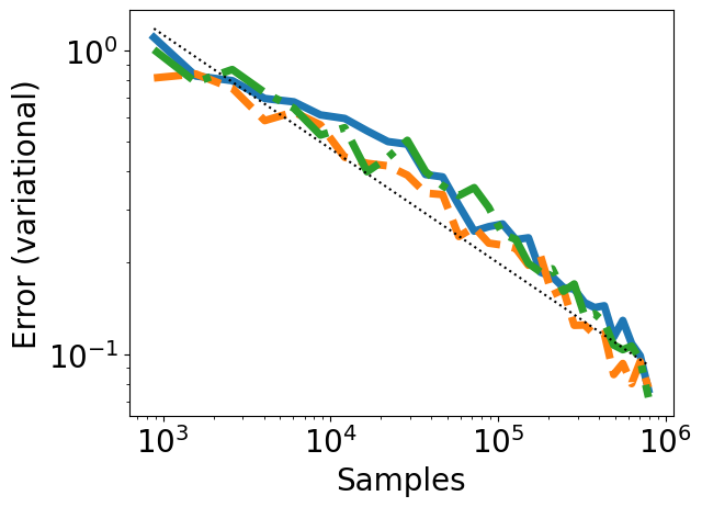
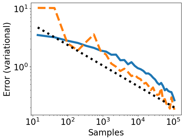
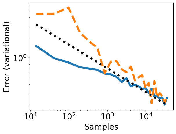
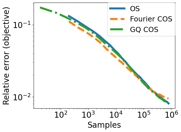
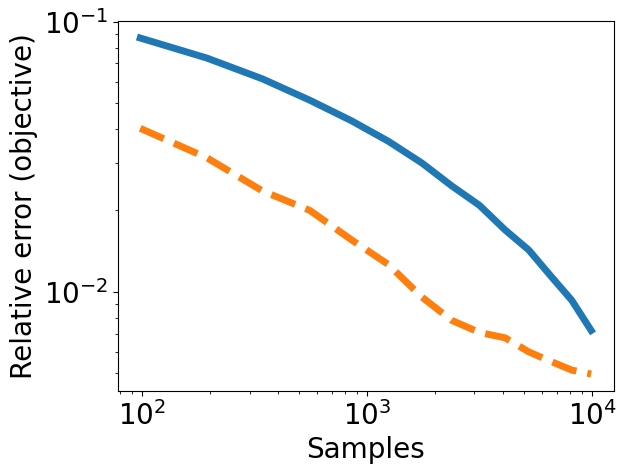
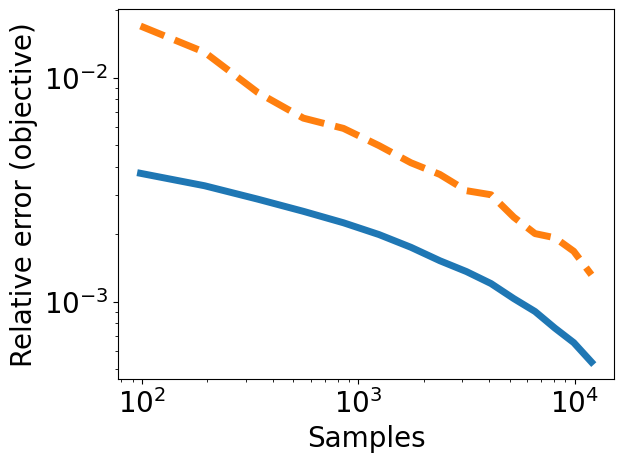
Figure 2: (a) $\varepsilon=0.4$, $a=1.5$, $b=-0.6$, $d=1$. Execution times: OS is $367s$, Fourier COS is $130s$ and GQ COS is $151s$. (b) $\varepsilon=0.5$, $a=1.2$, $b=-0.6$, $d=2$. Execution times: OS is $433s$ and Fourier COS is $207s$. (c) $\varepsilon=0.5$, $a=1.2$ ; $b=-0.6$, $d=5$. Execution times: OS is $386s$ and Fourier COS is $92s$.

5 Conclusion and future work

In this paper, we revisited the online Sinkhorn algorithm and provided an updated convergence analysis. We also proposed to combine this algorithm with measure compression techniques and demonstrated both theoretical and practical gains. We focused on the use of Fourier moments as a compression technique, and this worked particularly well with quadratic costs due to the fast tail behaviour of $\exp(-x^{2})$. However, Fourier compression generally performs less well for non-quadratic costs (such as $C(x,y)=\left\|x-y\right\|_{1}$) due to the slower frequency decay of $\exp(-C)$. We leave investigations into compression of such losses with slow tail behaviour as future work. Another direction of future work is to further investigate the non-asymptotic convergence behaviour: In Theorem 1, there is a linear convergence term which dominates in the non-asymptotic regime and it could be beneficial to adaptively choose the parameters $a,b$ to exploit this fast initial behaviour.

Appendix A Appendix

A.1 Gaussian mixture model

For experiments (b) and (c) in Figure 2, we set up test distributions $\alpha,\beta$ that sample from $\mathcal{N}(\mu_{i},\Sigma_{i})$ for $i=1,2$ with equal probability. For (b), the entries of $\mu_{1}$ are iid samples from $\mathcal{N}(0,100)$ for $\alpha$, and from $\mathcal{N}(0,25)$ for $\beta$; we take $\mu_{2}=-\mu_{1}$ in both cases. The covariance matrices $\Sigma_{i}=c_{i}\,QQ^{T}$ for $Q$ with iid standard Gaussian entries using $c_{1}=3$ and $c_{2}=4$. For (c), the same set-up is used with $c_{1}=1$ and $c_{2}=0.4$.

A.2 Useful lemmas

Define the operator $T_{\mu}$ to be [Mensch and Peyré, 2020]

$$T_{\mu}\left(h\right)=-\log\int_{y\in\mathcal{X}}\exp\left(h(y)-C\left(\cdot,y\right)\right)\mathrm{d}\mu(y),$$ (23)

then the updates with respect to the potentials $\left(f_{t},g_{t}\right)$ are

$$f_{t+1}=T_{\beta}(g_{t})\quad\text{and}\quad g_{t+1}=T_{\alpha}(f_{t}).$$ (24)

Under Assumption 1, a soft $C$-transform is always Lipschitz, and the following result can be found in [Vialard, 2019, Proposition 15].

Lemma 4.

Under Assumption 1, a soft $C$-transform $f=T_{\mu}(g)$ with a probability measure $\mu$ is $\varepsilon L$-Lipschitz, where $L$ is the Lipschitz constant of $C$ defined in Assumption 1.

We also show that the error $\underset{x\in\mathcal{X}}{\sup}\left\lvert f_{t}-f^{*}\right\rvert,\underset{x\in\mathcal{X}}{\sup}\left\lvert g_{t}-g^{*}\right\rvert$ in the online Sinkhorn is uniformly bounded.

Lemma 5.

Suppose for some $t>0$, $\max\left\{\underset{x\in\mathcal{X}}{\sup}\left\lvert f_{t}-f^{*}\right\rvert<\delta,\underset{y\in\mathcal{X}}{\sup}\left\lvert g_{t}-g^{*}\right\rvert\right\}<\delta$, where $\left(f^{*},g^{*}\right)$ is the pair of optimal potentials. Let $\left(f_{t+1},g_{t+1}\right)$ be the pair of potentials in the following updates

$$\exp\left(-f_{t+1}(x)/\varepsilon\right) =\left(1-\eta_{t}\right)\exp\left(-f_{t}(x)/\varepsilon\right)+\eta_{t}\int\exp\left(\left(g_{t}(y)-C(x,y)\right)/\varepsilon\right)\mathrm{d}\hat{\beta}_{t}(y),$$ (25)

$$\exp\left(-g_{t+1}(x)/\varepsilon\right) =\left(1-\eta_{t}\right)\exp\left(-g_{t}(x)/\varepsilon\right)+\eta_{t}\int\exp\left(\left(f_{t+1}(y)-C(x,y)\right)/\varepsilon\right)\mathrm{d}\hat{\alpha}_{t}(x),$$ (26)

where $\hat{\alpha}_{t},\hat{\beta}_{t}$ are two probability measures. Then $\underset{x\in\mathcal{X}}{\sup}\left\lvert f_{t+1}-f^{*}\right\rvert<\delta$.

Proof.

Multiply by $\exp{\left(f^{*}/\varepsilon\right)}$ on both sides of the equation 25,

$$\exp(f^{*}/\varepsilon-f_{t+1}/\varepsilon) =(1-\eta_{t})\exp(f^{*}/\varepsilon-f_{t}/\varepsilon)+\eta_{t}\int\exp((f^{*}+g_{t}-C)/\varepsilon)\mathrm{d}\hat{\beta}_{t},$$

$$=(1-\eta_{t})\exp(f^{*}/\varepsilon-f_{t}/\varepsilon)+\eta_{t}\int\exp((f^{*}+g^{*}-g^{*}+g_{t}-C)/\varepsilon)\mathrm{d}\hat{\beta}_{t},$$

$$=(1-\eta_{t})\exp(f^{*}/\varepsilon-f_{t}/\varepsilon)+\eta_{t}\int\exp((g_{t}-g^{*})/\varepsilon)\mathrm{d}\hat{\beta}_{t}$$

$$<(1-\eta_{t})\exp{\left(\delta/\varepsilon\right)}+\eta_{t}\int\exp{\left(\delta/\varepsilon\right)}\mathrm{d}\hat{\beta}_{t}=\exp{\left(\delta/\varepsilon\right)}.$$

Take logs on both sides to get $\underset{x\in\mathcal{X}}{\sup}\left\lvert f^{*}-f_{t+1}\right\rvert<\delta$. A similar argument gives the lower bound and we see that $\underset{x\in\mathcal{X}}{\sup}\left\lvert f^{*}-f_{t+1}\right\rvert<\delta$. ∎

As an example of [Van der Vaart, 2000, Chapter 19], we have the following results for function $\varphi(x)=\int\exp\left(\left(f(x)+g(y)-C(x,y)\right)/\varepsilon\right)\mathrm{d}\beta(y)$.

Lemma 6.

Under Assumption 1, let $y_{1},\cdots,y_{n}$ be i.i.d. random samples from a probability distribution $\beta$ on $\mathcal{X}$, and define for Lipschitz functions $f$ and $g$,

$$\varphi_{i}(x)=\exp\left(\left(f(x)+g(y_{i})-C(x,y_{i})\right)/\varepsilon\right),$$

$$\varphi(x)=\int\exp\left(\left(f(x)+g(y)-C(x,y)\right)/\varepsilon\right)\mathrm{d}\beta(y).$$ (27)

Suppose that $\left\|\exp\left(\left(f(x)+g(y)-C(x,y)\right)/\varepsilon\right)\right\|_{\infty}\leqslant M$ for some $M>0$, where $\left\|\cdot\right\|_{\infty}$ is the supremum norm. Then there exists $A>0$ depending on $f,g,\varepsilon$ such that, for all $n>0$,

$$\mathbb{E}\sup_{x\in\mathcal{X}}\left|\frac{1}{n}\sum_{i=1}^{n}\varphi_{i}(x)-\varphi(x)\right|\leqslant\frac{A}{\sqrt{n}}.$$

Moreover, $\underset{x\in\mathcal{X}}{\sup}\left|\frac{1}{n}\sum_{i=1}^{n}\varphi_{i}(x)-\varphi(x)\right|\xrightarrow{\text{a.s.}}0$ as $n\to\infty$.

Make use of Lemma 6 to further prove the difference of two $T_{\beta}(g)$ and $T_{\hat{\beta}}(g)$ has an upper bound in $\left\|\cdot\right\|_{var}$.

Lemma 7.

Suppose that $g$ is Lipshitcz and $\left(f^{*},g^{*}\right)$ is the pair of optimal potentials. Denote  $\zeta_{\hat{\beta}}\left(x\right)\stackrel{{\scriptstyle\mbox{\tiny def.}}}{{=}}\frac{\left(T_{\beta}(g)-T_{\hat{\beta}}(g)\right)}{\varepsilon}\left(x\right)$, where $\hat{\beta}=\frac{1}{n}\sum_{i=1}^{n}\delta_{y_{i}}$ is an empirical probability measure with $y_{i}\overset{\mathrm{iid}}{\sim}\beta$, $n\in\mathbb{Z}_{+}$, and $M\left(x\right)=\int\exp\left(\left(f^{*}\left(x\right)+g\left(y\right)-C\left(x,y\right)\right)/\varepsilon\right)\mathrm{d}\beta\left(y\right)$ is bounded from above and below with respect to $x$.

Then, there exists a constant $A_{1}(f^{*},g^{*},\varepsilon)$ depending on $f^{*},g^{*},\varepsilon$, such that

$$\mathbb{E}\|\zeta_{\hat{\beta}}\|_{var}\lesssim\frac{A_{1}(f^{*},g^{*},\varepsilon)}{\sqrt{n}}.$$ (28)

Proof.

For all $x\in\mathcal{X}$, using that $f^{*}=T_{\beta}(g^{*})$,

$$\left\|\zeta_{\hat{\beta}}\right\|_{var} =\left\|\left(T_{\beta}(g)-T_{\hat{\beta}}(g)\right)/\varepsilon\right\|_{var}=\left\|\log\left(\frac{\exp\left(-T_{\hat{\beta}}(g)/\varepsilon\right)}{\exp\left(-T_{\beta}(g)/\varepsilon\right)}\right)\right\|_{var}$$

$$=\left\|\log\left(1+\frac{\exp\left(-T_{\hat{\beta}}(g)/\varepsilon\right)-\exp\left(-T_{\beta}(g)/\varepsilon\right)}{\exp\left(-T_{\beta}(g)/\varepsilon\right)}\right)\right\|_{var}$$

$$=\left\|\log\left(1+\frac{\frac{1}{n}\sum_{i=1}^{n}\varphi_{i}-\varphi}{\int\exp\left((f^{*}+g-C)/\varepsilon\right)d\beta}\right)\right\|_{var}$$

$$=\left\|\log\left(1+\frac{\frac{1}{n}\sum_{i=1}^{n}\varphi_{i}-\varphi}{M}\right)\right\|_{var},$$

where $\varphi_{i}(x)=\exp\left((f^{*}(x)+g(y_{i})-C(x,y_{i}))/\varepsilon\right)$ and $\varphi(x)=\int\exp\left((f^{*}(x)+g(y)-C(x,y))/\varepsilon\right)\mathrm{d}\beta(y)$. Note that for any $x$

$$\frac{\frac{1}{{n}}\sum_{i=1}^{n}\varphi_{i}(x)-\varphi(x)}{M\left(x\right)}=\frac{\exp\left(-T_{\hat{\beta}}(g)/\varepsilon\right)}{\exp\left(-T_{\beta}(g)/\varepsilon\right)}-1>-1.$$

Let $B\left(x\right)=\frac{\frac{1}{{n}}\sum_{i=1}^{n}\varphi_{i}(x)-\varphi(x)}{M\left(x\right)}$, then $\|\zeta_{\hat{\beta}}\|_{var}\leqslant 2\|\zeta_{\hat{\beta}}\|_{\infty}=2\left\|\log\left(1+B\right)\right\|_{\infty}$.

By Lemma 6 and the assumption that $n$ is lower bounded, $\frac{1}{n}\sum_{i=1}^{n}\varphi_{i}(x)-\varphi(x)$ is upper bounded with respect to $x$. Hence, there exists $-1<L<U$, such that $L<B\left(x\right)<U$ for any $x$. Therefore, for any $x$

$$\log(1+L)<\log\left(1+B\left(x\right)\right)<\log(1+U),$$

and $\|\zeta_{\hat{\beta}}\|_{var}<2\max\{|\log(1+L)|,|\log(1+U)|\}\coloneqq Q$ for all $t$.

On the event $\Omega_{t}=\left\{B\left(x\right)\leqslant\frac{1}{2}\right\}$, by applying $\log(1+y)\leqslant-\log(1-y)\leqslant 2y$ for $0\leqslant y\leqslant\frac{1}{2}$

$$\|\zeta_{\hat{\beta}}\|_{var}\leqslant 2\max\left\{\log\left(1+B\left(x\right)\right),-\log\left(1-B\left(x\right)\right)\right\}=-2\log(1-B\left(x\right))\leqslant 4B\left(x\right).$$

By the Markov inequality, $\mathbb{P}\left[B>\frac{1}{2}\right]\leqslant 2\mathbb{E}(B)$. Split the expectation $\mathbb{E}\left[\|\zeta_{\hat{\beta}}\|_{var}\right]$ into two parts, by Lemma 6 and the fact that $M$ is bounded from above and below with respect to $x$, there exists a constant $A_{1}(f^{*},g^{*},\varepsilon)$ depending on $f^{*},g^{*},\varepsilon$,

$$\begin{split}\mathbb{E}\|\zeta_{\hat{\beta}}\|_{var}&=\mathbb{P}\left[B\leqslant\frac{1}{2}\right]\mathbb{E}\left[\|\zeta_{\hat{\beta}}\|_{var}\middle|B\leqslant\frac{1}{2}\right]+\mathbb{P}\left[B>\frac{1}{2}\right]\mathbb{E}\left[\|\zeta_{\hat{\beta}}\|_{var}\middle|B>\frac{1}{2}\right]\\ &\leqslant\mathbb{E}(4B+2BQ)=(4+2Q)\mathbb{E}B\\ &\lesssim\frac{A_{1}(f^{*},g^{*},\varepsilon)}{\sqrt{n}}.\end{split}$$ (29)

∎

The following lemma shows that the error in the variational norm at this step can be bounded using the error in the variational norm from the last step.

Lemma 8.

Given the empirical measures $\hat{\alpha}=\frac{1}{n}\sum_{i=1}^{n}\delta_{x_{i}}$, $\hat{\beta}=\frac{1}{n}\sum_{i=1}^{n}\delta_{y_{i}}$, where $x_{i}\overset{\mathrm{iid}}{\sim}\alpha$, $y_{i}\overset{\mathrm{iid}}{\sim}\beta$ and $n\in\mathbb{Z}_{+}$. Let $f,g$ be functions of  $C$-transform, consider the update in the online Sinkhorn algorithm for $\eta_{t}$ at step $t$,

$$\exp(-\hat{f}(x)/\varepsilon) =(1-\eta_{t})\exp(-f(x)/\varepsilon)+\eta_{t}\int\exp((g(y)-C(x,y))/\varepsilon)\mathrm{d}\hat{\beta}(y),$$ (30)

$$\exp(-\hat{g}(x)/\varepsilon) =(1-\eta_{t})\exp(-g(x)/\varepsilon)+\eta_{t}\int\exp((\hat{f}(y)-C(x,y))/\varepsilon)\mathrm{d}\hat{\alpha}(x).$$ (31)

Denote $U\stackrel{{\scriptstyle\mbox{\tiny def.}}}{{=}}\left(f-f^{*}\right)/\varepsilon$, $V\stackrel{{\scriptstyle\mbox{\tiny def.}}}{{=}}\left(g-g^{*}\right)/\varepsilon$, $\hat{U}\stackrel{{\scriptstyle\mbox{\tiny def.}}}{{=}}\left(\hat{f}-f^{*}\right)/\varepsilon$, $\hat{V}\stackrel{{\scriptstyle\mbox{\tiny def.}}}{{=}}\left(\hat{g}-g^{*}\right)/\varepsilon$, $\zeta_{\hat{\beta}}\stackrel{{\scriptstyle\mbox{\tiny def.}}}{{=}}\left(T_{\beta}(g)-T_{\hat{\beta}}(g)\right)/\varepsilon$, and $\iota_{\hat{\alpha}}\stackrel{{\scriptstyle\mbox{\tiny def.}}}{{=}}\left(T_{\alpha}(\hat{f})-T_{\hat{\alpha}}(\hat{f})\right)/\varepsilon$, then for $t$ large enough,

$$\|\hat{U}\|_{var}+\|\hat{V}\|_{var}\leqslant\left(1-\eta_{t}+\eta_{t}\kappa\right)\left(\|U\|_{var}+\|V\|_{var}\right)+\eta_{t}\left(\|\zeta_{\hat{\beta}}\|_{var}+\|\iota_{\hat{\alpha}}\|_{var}\right).$$ (32)

Proof.

Multiply $\exp\left(f^{*}/\varepsilon\right)$ on both sides on equation 30 we get

$$\exp\left((-\hat{f}+f^{*})/\varepsilon\right) =(1-\eta_{t})\exp\left((-f+f^{*})/\varepsilon\right)+\eta_{t}\exp\left(f^{*}(x)/\varepsilon\right)\int\exp\left((g(y)-C(x,y))/\varepsilon\right)\mathrm{d}\hat{\beta}(y)$$

$$=(1-\eta_{t})\exp\left((-f+f^{*})/\varepsilon\right)+\eta_{t}\exp{\left(-T_{\hat{\beta}}(g)/\varepsilon+T_{\beta}(g^{*})/\varepsilon\right)}$$

$$=(1-\eta_{t})\exp\left((-f+f^{*})/\varepsilon\right)+\eta_{t}\exp{\left(\left(T_{\beta}(g)-T_{\beta}(g)-T_{\hat{\beta}}(g)+T_{\beta}(g^{*})\right)/\varepsilon\right)}$$

$$=(1-\eta_{t})\exp\left((-f+f^{*})/\varepsilon\right)+\eta_{t}\exp\left(-T_{\beta}(g)/\varepsilon+T_{\beta}(g^{*})/\varepsilon+\zeta_{\hat{\beta}}\right),$$

and similarly, multiply $\exp\left(g^{*}/\varepsilon\right)$ on both sides of equation 31,

$$\exp\left((-\hat{g}+g^{*})/\varepsilon\right)=(1-\eta_{t})\exp\left((-g+g^{*})/\varepsilon\right)+\eta_{t}\exp\left(-T_{\alpha}(\hat{f})/\varepsilon+T_{\alpha}(f^{*})/\varepsilon+\iota_{\hat{\alpha}}\right)$$ (33)

where $(f^{*},g^{*})$ is the pair of optimal potentials.

Denote $\hat{U}^{T}\stackrel{{\scriptstyle\mbox{\tiny def.}}}{{=}}\left(T_{\alpha}(\hat{f})-T_{\alpha}(f^{*})\right)/\varepsilon$ and $V^{T}\stackrel{{\scriptstyle\mbox{\tiny def.}}}{{=}}\left(T_{\beta}(g)-T_{\beta}(g^{*})\right)/\varepsilon$. Then, we can find an upper bound for $\max\hat{U}$,

$$\max\hat{U} =-\log\min\exp(-\hat{U})$$

$$=-\log\left(\min\left((1-\eta_{t})\exp(-U)+\eta_{t}\exp(-V^{T}+\zeta_{\hat{\beta}})\right)\right)\qquad\text{by the update equation~{}\ref{eq1:C-transfer_updates}}$$

$$\leqslant-\log\left((1-\eta_{t})\min\exp(-U)+\eta_{t}\min\exp(-V^{T}+\zeta_{\hat{\beta}})\right)\qquad\text{by }\min f_{1}+\min f_{2}\leqslant\min(f_{1}+f_{2})$$

$$\leqslant-\left(1-\eta_{t}\right)\log\min\exp(-U)-\eta_{t}\log\min\exp(-V^{T}+\zeta_{\hat{\beta}})\qquad\text{by Jensen Inequality}$$

$$=\left(1-\eta_{t}\right)\max U+\eta_{t}\max\left(V^{T}-\zeta_{\hat{\beta}}\right),$$

and similarly,

$$\min\hat{U} \geqslant\left(1-\eta_{t}\right)\min U+\eta_{t}\min\left(V^{T}-\zeta_{\hat{\beta}}\right),$$

$$\max\hat{V} \leqslant\left(1-\eta_{t}\right)\max V+\eta_{t}\max\left(\hat{U}^{T}-\iota_{\hat{\alpha}}\right),$$

$$\min\hat{V} \geqslant\left(1-\eta_{t}\right)\min V+\eta_{t}\min\left(\hat{U}^{T}-\iota_{\hat{\alpha}}\right).$$

Therefore, by the contractivity of the soft-$C$ transform [Vialard, 2019, Proposition 19] that there exists a contractivity constant $\kappa<1$ such that $\left\|V^{T}\right\|_{var}\leqslant\kappa\left\|V\right\|_{var}$ and $\left\|\hat{U}^{T}\right\|_{var}\leqslant\kappa\left\|\hat{U}\right\|_{var}$ for any $t$,

$$\|\hat{U}\|_{var} \leqslant(1-\eta_{t})\|U\|_{var}+\eta_{t}\|V^{T}\|_{var}+\eta_{t}\|\zeta_{\hat{\beta}}\|_{var}$$

$$\leqslant(1-\eta_{t})\|U\|_{var}+\eta_{t}\kappa\|V\|_{var}+\eta_{t}\|\zeta_{\hat{\beta}}\|_{var}$$ (34)

$$\|\hat{V}\|_{var} \leqslant(1-\eta_{t})\|V\|_{var}+\eta_{t}\|\hat{U}^{T}\|_{var}+\eta_{t}\|\iota_{\hat{\alpha}}\|_{var}$$

$$\leqslant(1-\eta_{t})\|V\|_{var}+\eta_{t}\kappa\|\hat{U}\|_{var}+\eta_{t}\|\iota_{\hat{\alpha}}\|_{var}.$$ (35)

Substitute equation 34 into the RHS of equation 35,

$$\begin{split}\|\hat{V}\|_{var}&\leqslant(1-\eta_{t})\|V\|_{var}+\eta_{t}\kappa\left((1-\eta_{t})\|U\|_{var}+\eta_{t}\kappa\|V\|_{var}+\eta_{t}\|\zeta_{\hat{\beta}}\|_{var}\right)+\eta_{t}\|\iota_{\hat{\alpha}}\|_{var}\\ &=\left(1-\eta_{t}+\eta_{t}^{2}\kappa^{2}\right)\|V\|_{var}+(1-\eta_{t})\eta_{t}\kappa\|U\|_{var}+\eta_{t}^{2}\kappa\|\zeta_{\hat{\beta}}\|_{var}+\eta_{t}\|\iota_{\hat{\alpha}}\|_{var}.\end{split}$$ (36)

Add up equation 34 and equation 36

$$\left\|\hat{U}\right\|_{var}+\left\|\hat{V}\right\|_{var}\leqslant (1-\eta_{t}+\eta_{t}\kappa-\eta_{t}^{2}\kappa)\|U\|_{var}+\left(1-\eta_{t}+\eta_{t}\kappa+\eta_{t}^{2}\kappa^{2}\right)\|V\|_{var}$$

$$+\left(\eta_{t}+\eta_{t}^{2}\kappa\right)\|\zeta_{\hat{\beta}}\|_{var}+\eta_{t}\|\iota_{\hat{\alpha}}\|_{var}.$$

For $t$ large enough,

$$\|\hat{U}\|_{var}+\|\hat{V}\|_{var}\leqslant\left(1-\eta_{t}+\eta_{t}\kappa\right)\left(\|U\|_{var}+\|V\|_{var}\right)+\eta_{t}\left(\|\zeta_{\hat{\beta}}\|_{var}+\|\iota_{\hat{\alpha}}\|_{var}\right),$$ (37)

which holds for a possibly increased value of $\kappa$, as $\eta_{t}^{2}$ is negligible compared to $\eta_{t}$. ∎

Making use of a discrete version of Gronwall’s lemma [Mischler, 2018, Lemma 5.1], we are able to show the upper bound of $a_{t}$ by the recursion relation $a_{t+1}\lesssim\left(1-\eta_{t}+\eta_{t}\kappa\right)a_{t}+t^{\theta}$.

Lemma 9.

Given a sequence $a_{n}$ such that $a_{t+1}\lesssim\left(1-\eta_{t}+\eta_{t}\kappa\right)a_{t}+t^{\theta}$. Then

$$a_{t+1}\lesssim\left(a_{1}+C_{1}\right)\exp\left(C_{2}t^{b+1}\right)+t^{\theta-b},$$ (38)

where $C_{1}=\frac{1}{-\theta-1}>0$ and $C_{2}=\frac{\kappa-1}{b+1}<0$

Proof.

Summing over $t$, by the discrete version of Gronwall lemma [Mischler, 2018, Lemma 5.1], we have

$$a_{t+1}\lesssim \prod_{i=1}^{t}\left(1-\eta_{i}+\eta_{i}\kappa\right)a_{1}+\sum_{i=1}^{t-1}\left(\prod_{j=i+1}^{t}\left(1-\eta_{j}+\eta_{j}\kappa\right)\right)i^{\theta}+t^{\theta}$$

$$\stackrel{{\scriptstyle\mbox{\tiny def.}}}{{=}} A_{1,t}a_{1}+A_{2,t}+t^{\theta},$$

where

$$A_{1,t} =\prod_{i=1}^{t}\left(1-\eta_{i}+\eta_{i}\kappa\right),$$

$$A_{2,t} =\sum_{i=1}^{t-1}\left(\prod_{j=i+1}^{t}\left(1-\eta_{j}+\eta_{j}\kappa\right)\right)i^{\theta}.$$

First consider the term $A_{1,t}$, and taking the logarithm on it, using $\log\left(1+x\right)<x$,

$$\begin{split}\log A_{1,t}&=\sum_{i=1}^{t}\log\left(1+\left(\kappa-1\right)\eta_{i}\right)\leqslant\sum_{i=1}^{t}\left(\kappa-1\right)\eta_{i}\\ &<\left(\kappa-1\right)\int_{1}^{t+1}x^{b}\mathrm{d}x=\frac{\kappa-1}{b+1}\left(\left(t+1\right)^{b+1}-1\right).\end{split}$$ (39)

Thus, $A_{1,t}\leqslant\exp\left(\frac{\kappa-1}{b+1}\left(\left(t+1\right)^{b+1}-1\right)\right)$.

Now, take a look at the term $A_{2,t}$. Following the proof of [Moulines and Bach, 2011, Theorem 1], for any $1<m<t-1$,

$$A_{2,t}=\sum_{i=1}^{m}\left(\prod_{j=i+1}^{t}\left(1-\eta_{j}+\eta_{j}\kappa\right)\right)i^{\theta}+\sum_{i=m+1}^{t-1}\left(\prod_{j=i+1}^{t}\left(1-\eta_{j}+\eta_{j}\kappa\right)\right)i^{\theta}.$$ (40)

The first term $\sum_{i=1}^{m}\left(\prod_{j=i+1}^{t}\left(1-\eta_{j}+\eta_{j}\kappa\right)\right)i^{\theta}\leqslant\exp\left(\sum_{j=m+1}^{t}\left(\kappa-1\right)\eta_{j}\right)\sum_{i=1}^{m}i^{\theta}$, and the second term

$$\begin{split}\sum_{i=m+1}^{t-1}\left(\prod_{j=i+1}^{t}\left(1-\eta_{j}+\eta_{j}\kappa\right)\right)i^{\theta}&\leqslant m^{\theta-b}\sum_{i=m+1}^{t-1}\prod_{j=i+1}^{t}\left(1-\left(1-\kappa\right)\eta_{j}\right)\eta_{i}\\ &=\frac{m^{\theta-b}}{1-\kappa}\sum_{i=m+1}^{t-1}\left[\prod_{j=i+1}^{t}\left(1-\left(1-\kappa\right)\eta_{j}\right)-\prod_{j=i}^{t}\left(1-\left(1-\kappa\right)\eta_{j}\right)\right]\\ &\leqslant\frac{m^{\theta-b}}{1-\kappa}\left[1-\prod_{j=m+1}^{t-1}\left(1-\left(1-\kappa\right)\eta_{j}\right)\right]<\frac{m^{\theta-b}}{1-\kappa}.\end{split}$$ (41)

Therefore,

$$A_{2,t} <\exp\left(\left(\kappa-1\right)\int_{m+1}^{t+1}x^{b}\mathrm{d}x\right)\int_{1}^{m}x^{\theta}\mathrm{d}x+\frac{m^{\theta-b}}{1-\kappa}$$

$$=\exp\left(\frac{\kappa-1}{b+1}\left(\left(t+1\right)^{b+1}-\left(m+1\right)^{b+1}\right)\right)\frac{m^{\theta+1}-1}{\theta+1}+\frac{m^{\theta-b}}{1-\kappa}.$$

Take $m=\frac{t}{2}$,

$$A_{2,t}\lesssim\exp\left(\frac{\kappa-1}{b+1}\left(\left(t+1\right)^{b+1}-\left(t/2\right)^{b+1}\right)\right)\frac{1}{-\theta-1}+\frac{t^{\theta-b}}{1-\kappa}.$$ (42)

Combine Equations equation 39 and equation 42

$$a_{t+1}\lesssim\left(a_{1}+\frac{1}{-\theta-1}\right)\exp\left(\frac{\kappa-1}{b+1}t^{b+1}\right)+t^{\theta-b}.$$ (43)

∎

A.3 Proof of Theorem 1

Proof.

Let $U_{t}\stackrel{{\scriptstyle\mbox{\tiny def.}}}{{=}}\left(f_{t}-f^{*}\right)/\varepsilon$, $V_{t}\stackrel{{\scriptstyle\mbox{\tiny def.}}}{{=}}\left(g_{t}-g^{*}\right)/\varepsilon$, $e_{t}\stackrel{{\scriptstyle\mbox{\tiny def.}}}{{=}}\|U_{t}\|_{var}+\|V_{t}\|_{var}$, $\zeta_{\hat{\beta}_{t}}\stackrel{{\scriptstyle\mbox{\tiny def.}}}{{=}}\left(T_{\beta}(g_{t})-T_{\hat{\beta}_{t}}(g_{t})\right)/\varepsilon$ and $\iota_{\hat{\alpha}_{t}}\stackrel{{\scriptstyle\mbox{\tiny def.}}}{{=}}\left(T_{\alpha}(f_{t+1})-T_{\hat{\alpha}_{t}}(f_{t+1})\right)/\varepsilon$. By Lemma 8,

$$e_{t+1}\leqslant\left(1-\eta_{t}+\eta_{t}\kappa\right)e_{t}+\eta_{t}\left(\|\zeta_{\beta_{t}}\|_{var}+\|\iota_{\alpha_{t}}\|_{var}\right).$$ (44)

Define $M_{t}=\int\exp((f^{*}+g_{t}-c)/\varepsilon)\mathrm{d}\beta$, then

$$M_{t} =\int\exp((f^{*}+g^{*}-g^{*}+g_{t}-c)/\varepsilon)\mathrm{d}\beta$$

$$=\int\exp((-g^{*}+g_{t})/\varepsilon)\mathrm{d}\beta,$$

and by Lemma 5, there exists $\delta=\sup_{x\in\mathcal{X}}|f_{t_{0}}-f^{*}|>0$ for $t_{0}<t$, such that $\exp(-\delta/\varepsilon)<M_{t}<\exp(\delta/\varepsilon)$. Apply Lemma 7,

$$\begin{split}\mathbb{E}\left\|\zeta_{\hat{\beta}_{t}}\right\|_{var}&\lesssim\frac{A_{1}(f^{*},g^{*},\varepsilon)}{\sqrt{b_{t}}},\\ \mathbb{E}\left\|\iota_{\hat{\alpha}_{t}}\right\|_{var}&\lesssim\frac{A_{2}(f^{*},g^{*},\varepsilon)}{\sqrt{b_{t}}},\end{split}$$ (45)

where $A_{1}(f^{*},g^{*},\varepsilon),A_{2}(f^{*},g^{*},\varepsilon)$ are constants depending on $f^{*},g^{*},\varepsilon$.

Denote $S=A_{1}(f^{*},g^{*},\varepsilon)+A_{2}(f^{*},g^{*},\varepsilon)$, then taking expectation on equation 44 with Equations equation 45

$$\begin{split}\mathbb{E}e_{t+1}&\leqslant\left(1-\eta_{t}+\eta_{t}\kappa\right)\mathbb{E}e_{t}+\eta_{t}\mathbb{E}\left(\|\zeta_{\beta_{t}}\|_{var}+\|\iota_{\alpha_{t}}\|_{var}\right)\\ &\lesssim\left(1-\eta_{t}+\eta_{t}\kappa\right)\mathbb{E}e_{t}+\frac{S\eta_{t}}{\sqrt{b_{t}}}.\end{split}$$ (46)

By Lemma 9, we have

$$\mathbb{E}e_{t+1}\lesssim\left(\mathbb{E}e_{1}+\frac{S}{a-b-1}\right)\exp\left(\frac{\kappa-1}{b+1}t^{b+1}\right)+t^{-a},$$ (47)

whose RHS converges to $0$ as $t\to\infty$

Consider the upper bound equation 47 for $\delta_{t+1}$,

$$\delta_{t+1}\lesssim\left(\delta_{1}+\frac{S}{a-b-1}\right)\exp\left(\frac{\kappa-1}{b+1}t^{b+1}\right)+t^{-a}.$$

Note that the total sample size at step $t$ is $n_{t}=\sum_{i=1}^{t}i^{2a}=O\left(t^{2a+1}\right)$, thus we can rewrite $t$ in terms of $n_{t}$, that is $t=n_{t}^{\frac{1}{2a+1}}$. The first term decays rapidly with the rate ${O}\left(\exp\left(-n^{\frac{b+1}{2a+1}}\right)\right)$, since $\frac{\kappa-1}{b+1}<0$. Taking $t(N)=\lfloor N^{\frac{1}{2a+1}}\rfloor$, then when $t^{\frac{b+1}{2a+1}}\gg 1$,

$$\delta_{N}\lesssim\left(\delta_{1}+\frac{S}{a-b-1}\right)\exp\left(\frac{\kappa-1}{b+1}N^{\frac{b+1}{2a+1}}\right)+N^{-\frac{a}{2a+1}}={O}\left(N^{-\frac{1}{2+1/a}}\right),$$

which is bounded by $O\left(N^{-1/2}\right)$. ∎

A.4 Proof of Theorem 2

Proof.

This proof follows up on the proof of Theorem 1.

Recall the following terms regarding $f_{t}$ and $g_{t}$,

$$U_{t}\stackrel{{\scriptstyle\mbox{\tiny def.}}}{{=}}\left(f_{t}-f^{*}\right)/\varepsilon, V_{t} \stackrel{{\scriptstyle\mbox{\tiny def.}}}{{=}}\left(g_{t}-g^{*}\right)/\varepsilon,$$

$$U_{t}^{T}\stackrel{{\scriptstyle\mbox{\tiny def.}}}{{=}}\left(T_{\alpha}(f_{t})-T_{\alpha}(f^{*})\right)/\varepsilon, V_{t}^{T} \stackrel{{\scriptstyle\mbox{\tiny def.}}}{{=}}\left(T_{\beta}(g_{t})-T_{\beta}(g^{*})\right)/\varepsilon,$$

and further define the corresponding terms regarding $\hat{f}_{t}$ and $\hat{g}_{t}$,

$$\hat{U}_{t}\stackrel{{\scriptstyle\mbox{\tiny def.}}}{{=}}\left(\hat{f}_{t}-f^{*}\right)/\varepsilon, \hat{V}_{t} \stackrel{{\scriptstyle\mbox{\tiny def.}}}{{=}}\left(\hat{g}_{t}-g^{*}\right)/\varepsilon,$$

$$\hat{U}_{t}^{T}\stackrel{{\scriptstyle\mbox{\tiny def.}}}{{=}}\left(T_{\alpha}(\hat{f}_{t})-T_{\alpha}(f^{*})\right)/\varepsilon, \hat{V}_{t}^{T} \stackrel{{\scriptstyle\mbox{\tiny def.}}}{{=}}\left(T_{\beta}(\hat{g}_{t})-T_{\beta}(g^{*})\right)/\varepsilon,$$

$$\hat{\zeta}_{\hat{\beta}_{t}}\stackrel{{\scriptstyle\mbox{\tiny def.}}}{{=}}\left(T_{\beta}(\hat{g}_{t})-T_{\hat{\beta}_{t}}(\hat{g}_{t})\right)/\varepsilon, \hat{\iota}_{\hat{\alpha}_{t}} \stackrel{{\scriptstyle\mbox{\tiny def.}}}{{=}}\left(T_{\alpha}(f_{t+1})-T_{\hat{\alpha}_{t}}(f_{t+1})\right)/\varepsilon.$$

Notice that under Assumption 4, $\left\|\left(f_{t}-\hat{f}_{t}\right)/\varepsilon\right\|_{var}=O\left(t^{-a+b}\right)$. Suppose that

$$\max\left\{\sup_{x}\left\lvert\hat{f}_{t}-f^{*}\right\rvert,\sup_{y}\left\lvert\hat{g}_{t}-g^{*}\right\rvert\right\}<\delta,$$

then by Lemma 5, $\underset{x}{\sup}\left\lvert f_{t+1}-f^{*}\right\rvert<\delta$. Thus,

$$\underset{x}{\sup}\left\lvert\hat{f}_{t+1}-f^{*}\right\rvert =\underset{x}{\sup}\left\lvert\hat{f}_{t+1}-f_{t+1}+f_{t+1}-f^{*}\right\rvert$$

$$\leqslant\underset{x}{\sup}\left\lvert f_{t+1}-f^{*}\right\rvert+\underset{x}{\sup}\left\lvert\hat{f}_{t+1}-f_{t+1}\right\rvert$$

$$\lesssim\underset{x}{\sup}\left\lvert f_{t+1}-f^{*}\right\rvert+t^{-a+b}<\delta+t^{-a+b}.$$

Let $\delta=\max\left\{\underset{x}{\sup}\left\lvert\hat{f}_{1}-f^{*}\right\rvert,\underset{y}{\sup}\left\lvert\hat{g}_{1}-g^{*}\right\rvert\right\}$, we have

$$\underset{x}{\sup}\left\lvert\hat{f}_{t+1}-f^{*}\right\rvert\leqslant\delta+\sum_{i=1}^{t}i^{-a+b},$$

which is bounded from above and below as $-a+b+1<0$.

Notice that $\hat{g}_{t}$ and $f_{t+1}$ are $\varepsilon L$-Lipschitz, and apply Lemma 7,

$$\mathbb{E}\left\|\zeta_{\hat{\beta}_{t}}\right\|_{var} \lesssim\frac{A_{1}(f^{*},g^{*},\varepsilon)}{\sqrt{b_{t}}},$$

$$\mathbb{E}\left\|\iota_{\hat{\alpha}_{t}}\right\|_{var} \lesssim\frac{A_{2}(f^{*},g^{*},\varepsilon)}{\sqrt{b_{t}}},$$

where $A_{1}(f^{*},g^{*},\varepsilon),A_{2}(f^{*},g^{*},\varepsilon)$ are constants depending on $f^{*},g^{*},\varepsilon$.

We have the following relation

$$\hat{U}_{t+1} =\left(\hat{f}_{t+1}-f_{t+1}\right)/\varepsilon+\left(f_{t+1}-f^{*}\right)/\varepsilon\stackrel{{\scriptstyle\mbox{\tiny def.}}}{{=}}\text{err}_{f_{t+1}}+u_{t+1},$$

$$\hat{V}_{t+1} =\left(\hat{g}_{t+1}-g_{t+1}\right)/\varepsilon+\left(g_{t+1}-g^{*}\right)/\varepsilon\stackrel{{\scriptstyle\mbox{\tiny def.}}}{{=}}\text{err}_{g_{t+1}}+V_{t+1},$$

where $\text{err}_{f_{t+1}}=\left(\hat{f}_{t+1}-f_{t+1}\right)/\varepsilon$ and $\text{err}_{g_{t+1}}=\left(\hat{g}_{t+1}-g_{t+1}\right)/\varepsilon$, and

$$\left\|\hat{U}_{t+1}\right\|_{var} \leqslant\left\|\text{err}_{f_{t+1}}\right\|_{var}+\left\|U_{t+1}\right\|_{var},$$ (48)

$$\left\|\hat{V}_{t+1}\right\|_{var} \leqslant\left\|\text{err}_{g_{t+1}}\right\|_{var}+\left\|V_{t+1}\right\|_{var}.$$ (49)

Recall from Theorem 1 that $e_{t}\stackrel{{\scriptstyle\mbox{\tiny def.}}}{{=}}\|U_{t}\|_{var}+\|V_{t}\|_{var}$, and define $\hat{e}_{t}\stackrel{{\scriptstyle\mbox{\tiny def.}}}{{=}}\|\hat{U}_{t}\|_{var}+\|\hat{V}_{t}\|_{var}$. By Lemma 8, for $t$ large enough

$$e_{t+1}\leqslant\left(1-\eta_{t}+\eta_{t}\kappa\right)\hat{e}_{t}+\eta_{t}\left(\|\hat{\zeta}_{\hat{\beta}_{t}}\|_{var}+\|\hat{\iota}_{\hat{\alpha}_{t}}\|_{var}\right).$$ (50)

Thus, by the inequalities equation 48 and equation 50,

$$\begin{split}\hat{e}_{t+1}&\leqslant e_{t+1}+\left\|\text{err}_{f_{t+1}}\right\|_{var}+\left\|\text{err}_{g_{t+1}}\right\|_{var}\\ &\leqslant\left(1-\eta_{t}+\eta_{t}\kappa\right)\hat{e}_{t}+\eta_{t}\left(\|\hat{\zeta}_{\hat{\beta}_{t}}\|_{var}+\|\hat{\iota}_{\hat{\alpha}_{t}}\|_{var}\right)+\left\|\text{err}_{f_{t+1}}\right\|_{var}+\left\|\text{err}_{g_{t+1}}\right\|_{var}\end{split}$$ (51)

Take expectations on both sides of equation 51, we have

$$\mathbb{E}\hat{e}_{t+1} \leqslant\mathbb{E}e_{t+1}+\left\|\text{err}_{f_{t+1}}\right\|_{var}+\mathbb{E}\left\|\text{err}_{g_{t+1}}\right\|_{var}$$

$$\lesssim\left(1-\eta_{t}+\eta_{t}\kappa\right)\mathbb{E}\hat{e}_{t}+\frac{S\eta_{t}}{\sqrt{b_{t}}}+\mathbb{E}\left\|\text{err}_{f_{t+1}}\right\|_{var}+\mathbb{E}\left\|\text{err}_{g_{t+1}}\right\|_{var},$$

where $S=A_{1}(f^{*},g^{*},\varepsilon)+A_{2}(f^{*},g^{*},\varepsilon)$.

Notice that $\left\|\text{err}_{f_{t+1}}\right\|_{var}=O\left(t^{-a+b}\right)$ under Assumptions 4 and 5. By Lemma 9 with $\theta=b-a$,

$$\mathbb{E}\hat{e}_{t+1}\lesssim\left(\mathbb{E}e_{1}+\frac{1}{-\theta-1}\right)\exp\left(\frac{\kappa-1}{b+1}t^{b+1}\right)+\frac{1}{\left(1-\kappa\right)}t^{-a},$$ (52)

where the right-hand side goes to $0$ as $t\to\infty$. ∎

A.5 Compression errors

A.5.1 Gauss quadrature (GQ)

A quadrature rule uses a sum of specific points with assigned weights as an approximation to an integral, which are optimal with respect to a certain polynomial degree of exactness [Gautschi, 2004]. The $m$-point Gauss quadrature rule for $\mu$ can be expressed as

$$\int_{\mathbb{R}}f\left(y\right)\mathrm{d}\mu(y)=\sum_{i=1}^{m}w_{i}f\left(\hat{y}_{i}\right)+R_{m}\left(f\right),$$

for weights $w_{i}$ and points $\hat{y}_{i}$, where the remainder term $R_{m}$ satisifes $R_{m}\left(\mathbb{P}_{2m-1}\right)=0$, and therefore the sum approximation on the RHS matches the integral value on the LHS for $f\in\mathbb{P}_{2m-1}$.

In general, by [Gautschi, 2004, Corollary to Theorem 1.48], the error term $R_{m}$ can be expressed as

$$R_{m}(f)=M\frac{f^{(2m)}(\xi)}{(2m)!},\quad\text{some $\xi\in\mathbb{R}$}$$

where $M=\int_{\mathbb{R}}\left[\pi_{n}\left(t;d\mu\right)\right]^{2}\mathrm{d}\mu\left(t\right)$ and $\pi_{n}\left(\cdot;d\mu\right)$ is the numerator polynomial [Gautschi, 2004, Definition 1.35].

In our case, $f=K_{x}/v_{t}$. Note that $K_{x}$ and $v_{t}$ are smooth (both have the same regularity as $e^{-C(x,y)/\varepsilon}$; see equation 8). Moreover, note that $v_{t}$ is uniformly bounded away from 0 since $g_{t}$ is uniformly bounded. For $K_{x}(\xi)=\exp\left(-\frac{C\left(x,\xi\right)}{\varepsilon}\right)$ and, by the closed form of Gaussian functions,

$$K_{x}^{(2m)}(\xi)=\left(\frac{1}{\varepsilon}\right)^{m}\exp\left(-\frac{\left(x-\xi\right)^{2}}{\varepsilon}\right)H_{2m}\left(\frac{x-\xi}{\sqrt{\varepsilon}}\right)=O\left(\frac{\left(2m\right)!}{m!\varepsilon^{m}}\right),$$

where $H_{n}$ is the Hermite polynomial of $n$th order. It follows, by the Leibniz rule and the Faa di Bruno formula that, $R_{m}\left(f\right)=O\left(\frac{1}{\varepsilon^{m}m!}\right)$. Hence,

$$u_{t}(x)-\hat{u}_{t}(x) =\int\frac{K_{x}}{v_{t}}(y)\mathrm{d}\mu(y)-\int\frac{K_{x}}{v_{t}}(y)\mathrm{d}\hat{\mu}(y)=O\left(\frac{1}{\varepsilon^{m}m!}\right).$$

Note that $f_{t}(x)=-\varepsilon\log(u_{t}(x))$. By the mean-value theorem, $|\log a-\log b|\leq\frac{1}{a}|a-b|$ for $0<a<b$. Further, $u_{t}$ is bounded away from zero (as a continuous and positive function on a compact set). Hence, we may find a Lipschitz constant $L^{\prime}$ such that $|f_{t}(x)-\hat{f}_{t}(x)|\leq L^{\prime}|u_{t}(x)-\hat{u}_{t}(x)|$ for all $x\in\mathcal{X}$. Hence, Assumption 4 holds for any $\zeta>0$.

A.5.2 Fourier method

Consider $C(x,y)=\|x-y\|^{2}$. Take Fourier moments of $\int\frac{K_{x}}{v_{t}}\left(y\right)\mathrm{d}\mu\left(y\right)$,

$$\int\exp\left(-ikx\right)\int\frac{K_{x}}{v_{t}}\left(y\right)d\mu\left(y\right)dx=\int\frac{\hat{K}_{y}(k)}{v_{t}(y)}\mathrm{d}\mu\left(y\right)=\sqrt{\varepsilon\pi}\exp\left(-\frac{\varepsilon k^{2}}{4}\right)\int\frac{\exp\left(-iky\right)}{v_{t}(y)}\mathrm{d}\mu\left(y\right),$$ (53)

as $\hat{K}_{y}(k)$ for $K_{x}\left(y\right)=\exp\left(-\frac{\left(x-y\right)^{2}}{\varepsilon}\right)$ is given by

$$\begin{split}\hat{K}_{y}(k)&=\int\exp\left(-ikx\right)\exp\left(-\frac{\left(x-y\right)^{2}}{\varepsilon}\right)dx\\ &=\exp\left(-iky\right)\int\exp\left(-ikz\right)\exp\left(-\frac{z^{2}}{\varepsilon}\right)dz\\ &=\exp\left(-iky\right)\sqrt{\varepsilon\pi}\exp\left(-\frac{\varepsilon k^{2}}{4}\right).\end{split}$$ (54)

By the Fourier inversion theorem,

$$u_{t}(x)=\exp\left(-f_{t}\left(x\right)/\varepsilon\right)=\int\exp\left(ikx\right)\sqrt{\varepsilon\pi}\exp\left(-\frac{\varepsilon k^{2}}{4}\right)\int\frac{\exp\left(-iky\right)}{v_{t}(y)}\mathrm{d}\mu\left(y\right)\mathrm{d}k.$$ (55)

The compression error becomes

$$u_{t}(x)-\hat{u}_{t}(x)=\int\frac{K_{x}}{v_{t}}(y)d\mu(y)-\int\frac{K_{x}}{v_{t}}(y)d\hat{\mu}(y)=\int\frac{\varphi_{x}\left(z\right)}{v_{t}\left(y\right)}\mathrm{d}z,$$ (56)

where

$$\varphi_{x}\left(k\right)=\exp\left(i\,z\,k\right)\sqrt{\varepsilon\pi}\exp\left(-\frac{\varepsilon k^{2}}{4}\right)\int\exp\left(-i\,k\,y\right)\mathrm{d}\left(\mu-\hat{\mu}\right)\left(y\right),$$ (57)

and note that, by construction, $\varphi_{x}\left(k\right)=0$ for all $k\in\Omega$. The problem of finding the compression thus becomes a problem of evaluating the integral $\int\varphi_{x}\left(z\right)\mathrm{d}z$. Similarly to Gauss quadrature, we want to find $k\in\Omega=\left\{k_{1},\cdots,k_{m}\right\}$ such that the $\frac{1}{m}\sum_{i=1}^{m}\varphi_{x}\left(k_{i}\right)$ is an approximation to $\int\varphi_{x}\left(z\right)\mathrm{d}z$.

Let $\Omega=\left\{k_{1},\cdots,k_{m}\right\}$ be the set of $n$ elements that are QMC sampled from $X\sim\mathcal{N}\left(0,\frac{2}{\varepsilon}I\right)$. In practice, we use the implementation of SciPy [Virtanen et al., 2020]. Define $\chi\left(z\right)=\exp\left(\frac{\varepsilon z^{2}}{4}\right)\varphi_{x}\left(z\right)$. Notice that

$$\begin{split}\mathbb{E}\left(\chi\left(X\right)\right)&=\int_{\mathbb{R}^{d}}\left(2\pi\right)^{-d/2}\left(2/\varepsilon\right)^{-d/2}\exp\left(-\frac{\varepsilon}{4}z^{2}\right)\psi\left(z\right)\mathrm{d}z\\ &=\left(\frac{4\pi}{\varepsilon}\right)^{-d/2}\int_{\mathbb{R}^{d}}\varphi_{x}\left(z\right)\mathrm{d}z,\end{split}$$ (58)

and thus,

$$\int_{\mathbb{R}^{d}}\varphi_{x}\left(z\right)\mathrm{d}z=\left(\frac{4\pi}{\varepsilon}\right)^{d/2}\mathbb{E}\chi\left(X\right).$$ (59)

Following [Kuo and Nuyens, 2016, Section 4.1], let $\Psi(x)$ denote the cumulative distribution functions for $\mathcal{N}(0,1)$. Then $\Psi(\sqrt{\frac{\varepsilon}{{2}}}X_{i})\sim\mathcal{U}(0,1)$ and

$$\mathbb{E}\left(\chi\left(X\right)\right)=\int_{[0,1]^{d}}\chi\left(A\Psi^{-1}\left(z\right)\right)\mathrm{d}z,$$ (60)

where $A=\sqrt{\frac{2}{\varepsilon}}I$, $\Psi^{-1}\left(z\right)=\left(\Psi^{-1}\left(z^{1}\right),\cdots,\Psi^{-1}\left(z^{d}\right)\right)$. Denote $h\left(z\right)=\chi\left(A\Psi^{-1}\left(z\right)\right)$, and $I_{d}\left(h\right)=\int_{[0,1]^{d}}h\left(z\right)\mathrm{d}t$, where $d$ is the dimension, and $Q_{m,d}\left(h\right)=\frac{1}{m}\sum_{i=1}^{m}h\left(k_{i}\right)$. As $y\in\mathcal{X}$, a compact domain, the first derivative of $\chi(k)$ is bounded and the integrand $h$ has bounded variation. Hence, by [Kuo and Nuyens, 2016, Section 1.3],

$$\left\lvert I_{d}\left(h\right)-Q_{m,d}\left(h\right)\right\rvert=O\left(\frac{\left\lvert\log m\right\rvert^{d}}{m}\right).$$ (61)

Given that for $k\in\Omega$, $\varphi_{x}\left(k\right)=0$ and hence, $Q_{m,d}\left(h\right)=0$. Then, we know

$$\begin{split}\int_{\mathbb{R}^{d}}\varphi_{x}\left(z\right)\mathrm{d}z=\left(\frac{4\pi}{\varepsilon}\right)^{d/2}I_{d}\left(h\right)&\leqslant\left(\frac{4\pi}{\varepsilon}\right)^{d/2}\left(Q_{m,d}\left(h\right)+\left\lvert I_{d}\left(h\right)-Q_{m,d}\left(h\right)\right\rvert\right)\\ &=O\left(\left(\frac{4\pi}{\varepsilon}\right)^{d/2}\frac{\left\lvert\log m\right\rvert^{d}}{m}\right).\end{split}$$ (62)

Choosing $k$ in equation 12 via Gaussian QMC, the compression error is then

$$u_{t}(x)-\hat{u}_{t}(x)=\exp\left(-f_{t}\left(x\right)/\varepsilon\right)-\exp\left(-\hat{f}_{t}\left(x\right)/\varepsilon\right)=O\left(\frac{\left\lvert\log m\right\rvert^{d}}{m}\right).$$ (63)

If we take $\zeta<1$, then $\frac{\left\lvert\log m\right\rvert^{d}}{m}=o\left(m^{-\zeta}\right)$. Again applying the Lipschitz argument, $f_{t}(x)-\hat{f}_{t}(x)=O\left(\frac{\left\lvert\log m\right\rvert^{d}}{m}\right)$ and Assumption 4 holds.

A.6 Proof of Proposition 3

Proof.

Cost of online Sinkhorn Now we calculate the complexity of Algorithm 2 up to step $T$. Recalled that in Section 2.2.1, the computational complexity of Algorithm 1 is $\mathcal{C}=O\left(dT^{4a+2}\right)$. By Theorem 1, the error at step $T$ is $\delta=O\left(T^{-a}\right)$ (where the hidden constant may depend on dimension). Taking $T=O(\delta^{-1/a})$, we have $\mathcal{C}=O\left(\delta^{-\left(4+\frac{2}{a}\right)}\right)$.

Cost of compressed online Sinkhorn

Assuming$m_{t}=t^{\frac{a-b}{\zeta}}$, the total computational cost of Algorithm 2 is

$$\hat{\mathcal{C}} =\sum_{t=1}^{T}\left(C(n_{t-1},m_{t})+db_{t}m_{t}\right)$$

$$=\sum_{t=1}^{T}\left(m_{t}^{3}+d\left(m_{t-1}+b_{t-1}\right)m_{t}+db_{t}m_{t}\right)$$

$$=O\left(\sum_{t=1}^{T}\left(t^{\frac{3\left(a-b\right)}{\zeta}}+d\left(t-1\right)^{2a}t^{\frac{a-b}{\zeta}}+dt^{2a+\frac{a-b}{\zeta}}\right)\right)$$

$$=\begin{cases}O\left(dT^{2a+\frac{a-b}{\zeta}+1}\right),&\text{ for }\zeta\geqslant\frac{a-b}{a}\\ O\left(T^{\frac{3\left(a-b\right)}{\zeta}+1}\right),&\text{ for }\zeta<\frac{a-b}{a}\end{cases}.$$

Under Assumptions 4 and 5, the error at step $T$ is $\delta=O\left(T^{-a}\right)$. Taking $T=\delta^{-1/a}$, we have

$$\hat{\mathcal{C}}=\begin{cases}O\left(\delta^{-\left(2+\frac{a-b}{a\zeta}+\frac{1}{a}\right)}\right),&\text{ for }\zeta\geqslant\frac{a-b}{a},\\ O\left(\delta^{-\left(\frac{3\left(a-b\right)}{a\zeta}+\frac{1}{a}\right)}\right),&\text{ for }\zeta<\frac{a-b}{a}.\end{cases}$$

The big-$O$ constant for the accuracy $\delta$ may depend on dimension. ∎

Notice that the ratio of $\hat{\mathcal{C}}$ and $\mathcal{C}$,

$$\frac{\hat{\mathcal{C}}}{\mathcal{C}}=\begin{cases}{O}\left(\delta^{2+\frac{1}{a}-\frac{a-b}{a\zeta}}\right),&\text{ for }\zeta\geqslant\frac{a-b}{a},\\ {O}\left(\delta^{4+\frac{1}{a}-\frac{3\left(a-b\right)}{a\zeta}}\right),&\text{ for }\zeta<\frac{a-b}{a},\end{cases}$$ (64)

and the exponent of the ratio is positive when $\zeta>\frac{3\left(a-b\right)}{4a+1}$, which means the asymptotical convergence of the Compressed Online Sinkhorn is improved compared to the Online Sinkhorn.

References

• [Adachi et al., 2022] Adachi, M., Hayakawa, S., Jørgensen, M., Oberhauser, H., and Osborne, M. A. (2022). Fast Bayesian inference with batch Bayesian quadrature via kernel recombination. Advances in Neural Information Processing Systems, 35:16533–16547.
• [Altschuler et al., 2019] Altschuler, J., Bach, F., Rudi, A., and Niles-Weed, J. (2019). Massively scalable Sinkhorn distances via the Nyström method. Advances in Neural Information Processing Systems, 32:4427–4437.
• [Altschuler et al., 2017] Altschuler, J., Weed, J., and Rigollet, P. (2017). Near-linear time approximation algorithms for optimal transport via Sinkhorn iteration. arXiv preprint arXiv:1705.09634.
• [Aude et al., 2016] Aude, G., Cuturi, M., Peyré, G., and Bach, F. (2016). Stochastic optimization for large-scale optimal transport. arXiv preprint arXiv:1605.08527.
• [Charlier et al., 2021] Charlier, B., Feydy, J., Glaunès, J. A., Collin, F.-D., and Durif, G. (2021). Kernel operations on the GPU, with autodiff, without memory overflows. Journal of Machine Learning Research, 22(74):1–6.
• [Cosentino et al., 2020] Cosentino, F., Oberhauser, H., and Abate, A. (2020). A randomized algorithm to reduce the support of discrete measures. Advances in Neural Information Processing Systems, 33:15100–15110.
• [Cuturi, 2013] Cuturi, M. (2013). Sinkhorn distances: Lightspeed computation of optimal transport. Advances in Neural Information Processing Systems, 26:2292–2300.
• [Ferradans et al., 2014] Ferradans, S., Papadakis, N., Peyré, G., and Aujol, J.-F. (2014). Regularized discrete optimal transport. SIAM Journal on Imaging Sciences, 7(3):1853–1882.
• [Gautschi, 2004] Gautschi, W. (2004). Orthogonal polynomials: computation and approximation. OUP Oxford.
• [Genevay et al., 2019] Genevay, A., Chizat, L., Bach, F., Cuturi, M., and Peyré, G. (2019). Sample complexity of Sinkhorn divergences. In The 22nd international conference on artificial intelligence and statistics, pages 1574–1583. PMLR.
• [Hayakawa et al., 2022] Hayakawa, S., Oberhauser, H., and Lyons, T. (2022). Positively weighted kernel quadrature via subsampling. Advances in Neural Information Processing Systems, 35:6886–6900.
• [Janati et al., 2020] Janati, H., Muzellec, B., Peyré, G., and Cuturi, M. (2020). Entropic optimal transport between unbalanced Gaussian measures has a closed form. Advances in Neural Information Processing Systems, 33:10468–10479.
• [Kantorovich, 1942] Kantorovich, L. (1942). On the transfer of masses (in Russian).
• [Kuo and Nuyens, 2016] Kuo, F. Y. and Nuyens, D. (2016). A practical guide to quasi-Monte Carlo methods. Lecture notes.
• [Mensch and Peyré, 2020] Mensch, A. and Peyré, G. (2020). Online Sinkhorn: Optimal transport distances from sample streams. arXiv e-prints, pages arXiv–2003.
• [Mischler, 2018] Mischler, S. (2018). Lecture notes: An Introduction to Evolution PDEs.
• [Moulines and Bach, 2011] Moulines, E. and Bach, F. (2011). Non-asymptotic analysis of stochastic approximation algorithms for machine learning. Advances in neural information processing systems, 24:451–459.
• [Ni et al., 2009] Ni, K., Bresson, X., Chan, T., and Esedoglu, S. (2009). Local histogram based segmentation using the Wasserstein distance. International journal of computer vision, 84:97–111.
• [Pedregosa et al., 2011] Pedregosa, F., Varoquaux, G., Gramfort, A., Michel, V., Thirion, B., Grisel, O., Blondel, M., Prettenhofer, P., Weiss, R., Dubourg, V., Vanderplas, J., Passos, A., Cournapeau, D., Brucher, M., Perrot, M., and Duchesnay, E. (2011). Scikit-learn: Machine learning in Python. Journal of Machine Learning Research, 12:2825–2830.
• [Peyré et al., 2019] Peyré, G., Cuturi, M., et al. (2019). Computational optimal transport: With applications to data science. Foundations and Trends® in Machine Learning, 11(5-6):355–607.
• [Schiebinger et al., 2019] Schiebinger, G., Shu, J., Tabaka, M., Cleary, B., Subramanian, V., Solomon, A., Gould, J., Liu, S., Lin, S., Berube, P., et al. (2019). Optimal-transport analysis of single-cell gene expression identifies developmental trajectories in reprogramming. Cell, 176(4):928–943.
• [Tchernychova, 2015] Tchernychova, M. (2015). Caratheodory cubature measures. PhD thesis, Oxford.
• [Van der Vaart, 2000] Van der Vaart, A. W. (2000). Asymptotic statistics, volume 3. Cambridge university press.
• [Vialard, 2019] Vialard, F.-X. (2019). An elementary introduction to entropic regularization and proximal methods for numerical optimal transport. Lecture notes.
• [Virtanen et al., 2020] Virtanen, P., Gommers, R., Oliphant, T. E., Haberland, M., Reddy, T., Cournapeau, D., Burovski, E., Peterson, P., Weckesser, W., Bright, J., van der Walt, S. J., Brett, M., Wilson, J., Millman, K. J., Mayorov, N., Nelson, A. R. J., Jones, E., Kern, R., Larson, E., Carey, C. J., Polat, İ., Feng, Y., Moore, E. W., VanderPlas, J., Laxalde, D., Perktold, J., Cimrman, R., Henriksen, I., Quintero, E. A., Harris, C. R., Archibald, A. M., Ribeiro, A. H., Pedregosa, F., van Mulbregt, P., and SciPy 1.0 Contributors (2020). SciPy 1.0: Fundamental Algorithms for Scientific Computing in Python. Nature Methods, 17:261–272.
• [Xu et al., 2020] Xu, J., Zhou, H., Gan, C., Zheng, Z., and Li, L. (2020). Vocabulary learning via optimal transport for neural machine translation. arXiv preprint arXiv:2012.15671.
• [Zhang et al., 2008] Zhang, K., Tsang, I. W., and Kwok, J. T. (2008). Improved Nyström low-rank approximation and error analysis. In Proceedings of the 25th international conference on Machine learning, pages 1232–1239.