A framework to generate sparsity-inducing regularizers for enhanced low-rank matrix completion

Abstract

Applying half-quadratic optimization to loss functions can yield the corresponding regularizers, while these regularizers are usually not sparsity-inducing regularizers (SIRs). To solve this problem, we devise a framework to generate an SIR with closed-form proximity operator. Besides, we specify our framework using several commonly-used loss functions, and produce the corresponding SIRs, which are then adopted as nonconvex rank surrogates for low-rank matrix completion. Furthermore, algorithms based on the alternating direction method of multipliers are developed. Extensive numerical results show the effectiveness of our methods in terms of recovery performance and runtime.

I Introduction

Low-rank matrix completion (LRMC) aims to fill the unobserved entries of an incomplete matrix with the use of the low-rank property [1]. It has numerous real-world applications such as image inpainting [2], hyperspectral image restoration [3] and collaborative filtering [4]. That is because although these data have high-dimensional structure, their main information lies in a subspace with a much lower dimensionality. Roughly speaking, two strategies are widely used for LRMC, namely, matrix factorization [5, 6] and rank minimization [7, 8]. The former formulates the estimated matrix as a product of two much smaller matrices, but it requires knowing the prior rank information, which may be not easy to determine in real-world scenarios.

Different from matrix factorization, the rank minimization can estimate the rank of the observed matrix via employing an SIR to make the singular values sparse [9, 10, 11]. One popular and feasible method is nuclear norm minimization (NNM) [7]. However, since NNM utilizes the $\ell_{1}$-norm to shrink all nonzero singular values by the same constant, the resultant solution is biased. To solve this issue, nonconvex sparsity-inducing regularizers (SIRs) are suggested because they have less estimation bias than the $\ell_{1}$-norm [13]. Many nonconvex SIRs are adopted to replace the $\ell_{1}$-norm for LRMC [9], while they cannot ensure that the resultant subproblems associated with these SIRs are convex, and the closed-from solutions to these subproblems are not obtained, implying high computational costs. To handle this problem, a parameterized nonconvex SIR is proposed in [12]. However, to maintain the convexity of the subproblem associated with this SIR, one parameter is required to be properly set. Moreover, Gu $et$ $al$. [14, 15] employ a weighted NNM (WNNM) for LRMC, yielding better low-rank recovery than the NNM.

On the other hand, it has been analyzed that applying half-quadratic (HQ) optimization [16] or the Legendre-Fenchel (LF) transform [17] to loss functions, including the Welsch, German-McClure (GMC) and Cauchy functions [18], can yield regularizers with closed-form proximity operators. However, these regularizers are usually not SIRs [19]. In this work, our attempt is to answer an interesting and important question: Under what conditions, the resultant regularizers are SIRs ?.

Motivated by the results in [3, 19, 20, 21], we devise a framework to generate SIRs with closed-form proximity operators. Note that the loss functions considered in [3, 19] are a special case of our framework. Besides, it is analyzed that the subproblems associated with our SIRs are convex with closed-form solutions and our SIRs can yield a less bias solution than the $\ell_{1}$-norm. We then employ the SIRs for LRMC, and algorithms based on the alternating direction method of multipliers (ADMM) are developed.

II Preliminaries

II-A Proximity Operator

The Moreau envelope of a regularizer $\varphi(\cdot)$ is defined as [22]:

$$\begin{split}\min\limits_{y}~{}\frac{1}{2}(x-y)^{2}+\lambda\varphi(y)\end{split}$$ (1)

whose solution is given by the proximity operator:

$$\begin{split}P_{\varphi}(x):={\rm\arg}\min\limits_{y}~{}\frac{1}{2}(x-y)^{2}+\lambda\varphi(y)\end{split}$$ (2)

In particular, when $\varphi(\cdot)=|\cdot|_{1}$, the solution to (1) is:

$$\begin{split}P_{\ell_{1},\lambda}(x)={\rm max}\{0,|x|-\lambda\}{\rm sign}(x)\end{split}$$ (3)

which is called the proximity operator of $|\cdot|_{1}$, also known as the soft-thresholding operator. From (3), it is clear that the $\ell_{1}$-norm is an SIR. Here, $\varphi(\cdot)$ is called an SIR if the solution to (1) is zero if the magnitude of $|x|$ is no bigger than a threshold. On the other hand, although applying the HQ optimization to the Welsch, Cauchy or GMC function can give the corresponding regularizer with closed-form proximity operator [18], the generated regularizers are not SIRs.

II-B Related Works

Given an incomplete matrix $\boldsymbol{X}_{\Omega}\in\mathbb{R}^{m\times n}$ with ${\Omega}\subset\{1,\cdots,m\}\times\{1,\cdots,n\}$ being the index set of the observed elements, defined as:

$$\left[\boldsymbol{X}_{\Omega}\right]_{ij}=\left\{\begin{aligned} &X_{ij},\quad{\rm if}~{}(i,j)\in\Omega\\ &0,\quad\quad{\rm if}~{}(i,j)\in\Omega^{c}\\ \end{aligned}\right.$$

where $\Omega^{c}$ is the complement of $\Omega$, LRMC can be solved by NNM [7]:

$$\begin{split}&\mathop{\min}\limits_{\boldsymbol{M}}~{}\|{\boldsymbol{M}}\|_{*},~{}\text{s.t.}~{}\boldsymbol{M}_{\Omega}=\boldsymbol{X}_{\Omega}\end{split}$$ (4)

where $\|\boldsymbol{M}\|_{*}=\sum_{i=1}^{r}\boldsymbol{\sigma}_{i}$ denotes the nuclear norm of the estimated matrix $\boldsymbol{M}$ and $\boldsymbol{\sigma}_{i}$ is the $i$th singular value of $\boldsymbol{M}$. Nevertheless, nuclear norm is equivalent to applying the $\ell_{1}$-norm to the singular value of a matrix, which shrinks all singular values with the same constant. However, as large singular values may dominate the main structure of real-world data, it is better to shrink them less [14]. Hence nonconvex SIRs have been suggested to replace the $\ell_{1}$-norm as nonconvex rank surrogates for LRMC [9]:

$$\begin{split}&\mathop{\min}\limits_{\boldsymbol{M}}~{}\|{\boldsymbol{M}}\|_{\varphi},~{}\text{s.t.}~{}\boldsymbol{M}_{\Omega}=\boldsymbol{X}_{\Omega}\end{split}$$ (5)

where $\|\boldsymbol{M}\|_{\varphi}=\sum_{i=1}^{r}\varphi{(\boldsymbol{\sigma}_{i})}$ and $\varphi(\cdot)$ is a nonconvex SIR. As shown in [10, 11], solving (5) involves the proximity operator of $\varphi(\cdot)$. However, existing SIRs, like the $\ell_{p}$-norm with $0<p<1$ except for $p=\{1/2,2/3\}$ [23], may not have the closed-form proximity operator, implying that iterations are needed for its computation. Furthermore, it is worth noting that when $\varphi{(\boldsymbol{\sigma}_{i})}=\boldsymbol{w}_{i}\boldsymbol{\sigma}_{i}$ with $\boldsymbol{w}_{i}$ being a weight parameter, $\|\boldsymbol{M}\|_{\varphi}$ is the weighted nuclear norm and (5) becomes the WNNM problem [14].

III Framework to Generate SIR and its Application to LRMC

As the Huber [20], truncated-quadratic [3] and hybrid ordinary-Welsch (HOW) [19] functions can yield SIRs using the LF transform, we generalize this class of functions and devise a framework to produce an SIR with closed-from proximity operator. Then, the generated SIR is considered as a nonconvex rank surrogate for LRMC.

III-A Framework to Generate SIRs

We first provide our framework in the following theorem.

Theorem 1.

Consider a continuously differentiable loss function $\phi_{h,\lambda}(x)$, defined as:

$$\phi_{h,\lambda}(x)=\begin{cases}x^{2}/2,&|x|\leq\lambda\\ a\cdot h(|x|)+b,&|x|\textgreater\lambda\end{cases}$$ (6)

where $a$ and $b$ are constants to make $\phi_{h,\lambda}(x)$ continuously differentiable, such that $g(x)=x^{2}/2-\phi_{h,\lambda}(x)$ is a proper, lower semi-continuous and convex function. Then it can be used to generate an SIR $\varphi_{h,\lambda}(\cdot)$ via LF transform, namely,

$$\phi_{h,\lambda}(x)=\mathop{\min}\limits_{y}~{}\frac{1}{2}(x-y)^{2}+\lambda\varphi_{h,\lambda}(y)$$ (7)

where $\varphi_{h,\lambda}(y)=\mathop{\max}\limits_{x}~{}\phi_{h,\lambda}(x)/\lambda-\frac{1}{2\lambda}(x-y)^{2}$. The solution to $y$ in (7) is given by the proximity operator:

$$P_{\varphi_{h,\lambda}}(x)=\nabla g={\rm max}\left\{0,|x|-a\cdot h^{\prime}(|x|)\right\}\cdot{\rm sign}(x)$$ (8)

Proof: The process of obtaining (8) and (7) from (6) is the same as that getting (16) and (17) from (9) in our previous work [19], and we omit the process due to page limit. $\hfill\blacksquare$

In addition, the expression of $\varphi_{h,\lambda}(\cdot)$ is generally unknown [16, 20], and its properties are provided in the following proposition.

Proposition 1.

$\varphi_{h,\lambda}(\cdot)$ has the following properties:

• Problem (7) is a convex problem although $\varphi_{h,\lambda}(y)$ is nonconvex.

• $P_{\varphi_{h,\lambda}}(x)$ is monotonically non-decreasing, namely, for any $x_{1}<x_{2}$, $P_{\varphi_{h,\lambda}}(x_{1})\leq P_{\varphi_{h,\lambda}}(x_{2})$.

• If $\phi_{h,\lambda}(x)$ is strictly concave for $x>\lambda$, the resultant proximity operator makes the solution have less bias than the proximity operator of the $\ell_{1}$-norm.

Proof: (i) can be obtained due to the conjugate theory, which is similar the proof of Proposition 1 in [19]. As $\phi_{h,\lambda}$ is an even function and the function $g$ is convex, we then have (ii). For (iii), the bias $\Delta b$ can be estimated by the gap between the identity function and the proximity operator for $|x|\geq\lambda$, and since the proximity operator is odd, we only discuss $\Delta b=x-P_{\varphi_{h,\lambda}}(x)=a\cdot h^{\prime}(x)$ for $x\geq\lambda$. Observing (3), it is apparent that the bias generated by the $\ell_{1}$-norm is $\lambda$. While when $x=\lambda$, the bias generated by our SIRs is $\lambda$, thus we need $\Delta b$ decreases with $x>\lambda$ to ensure that the bias produced by our SIRs is less than that by the $\ell_{1}$-norm. Therefore, we have $(\Delta b)^{\prime}=a\cdot h^{\prime\prime}(x)<0$, implying that $\phi_{h,\lambda}(x)$ is strictly concave for $x>\lambda$. $\hfill\blacksquare$

TABLE I: Different loss functions and their proximity operators.

	HOW	HOC	HOG
$l_{\cdot,\lambda}(x)$	$\begin{cases}x^{2}/2,&|x|\leq\lambda\\ \frac{\sigma^{2}}{2}\left(1-e^{\frac{\lambda^{2}-x^{2}}{\sigma^{2}}}\right)+\frac{\lambda^{2}}{2},&|x|\textgreater\lambda\end{cases}$	$\begin{cases}x^{2}/2,&|x|\leq\lambda\\ \frac{\gamma^{2}+\lambda^{2}}{2}\ln\left(1+\frac{x^{2}}{\gamma^{2}}\right)+\delta,&|x|\textgreater\lambda\end{cases}$	$\begin{cases}x^{2}/2,&|x|\leq\lambda\\ \frac{(\lambda^{2}+4\tau^{2})^{2}x^{2}}{8\tau^{2}(x^{2}+4\tau^{2})}-\frac{\lambda^{4}}{8\tau^{2}},&|x|\textgreater\lambda\end{cases}$
$l_{\cdot,\lambda}(x)$	$\mathop{\min}\limits_{y}~{}\frac{(x-y)^{2}}{2}+\lambda\varphi_{\sigma,\lambda}(y)$	$\mathop{\min}\limits_{y}~{}\frac{(x-y)^{2}}{2}+\lambda\varphi_{\gamma,\lambda}(y)$	$\mathop{\min}\limits_{y}~{}\frac{(x-y)^{2}}{2}+\lambda\varphi_{\tau,\lambda}(y)$
$P_{\varphi_{\cdot,\lambda}}(x)$	${\rm max}\left\{0,|x|-|x|e^{\frac{\lambda^{2}-x^{2}}{\sigma^{2}}}\right\}{\rm sign}(x)$	${\rm max}\left\{0,|x|-\frac{\left(\gamma^{2}+\lambda^{2}\right)|x|}{\gamma^{2}+x^{2}}\right\}{\rm sign}(x)$	${\rm max}\left\{0,|x|-\frac{(\lambda^{2}+4\tau^{2})^{2}|x|}{(x^{2}+4\tau^{2})^{2}}\right\}{\rm sign}(x)$

Next, we specify the function $g$ as the Welsch, GMC and Cauchy functions to develop the corresponding hybrid ordinary-Welsch (HOW), hybrid ordinary-GMC (HOG) and hybrid ordinary-Cauchy (HOC) functions, where ‘ordinary’ refers to the quadratic function, and the corresponding SIRs, namely, $\varphi_{\sigma,\lambda}(\cdot)$, $\varphi_{\gamma,\lambda}(\cdot)$ and $\varphi_{\tau,\lambda}(\cdot)$, which are shown in Table I. Moreover, by Proposition 1, to make the bias generated by our SIRs less than that by the $\ell_{1}$-norm, we have $\sigma\leq\sqrt{2}\lambda$, $\gamma\leq\lambda$ and $\tau\leq\sqrt{3}\lambda/2$ for $\varphi_{\sigma,\lambda}(\cdot)$, $\varphi_{\gamma,\lambda}(\cdot)$ and $\varphi_{\tau,\lambda}(\cdot)$, respectively. Fig. 1 plots the curves of $\varphi_{\sigma,\lambda}(\cdot)$, $\varphi_{\gamma,\lambda}(\cdot)$ and $\varphi_{\tau,\lambda}(\cdot)$ and their proximity operators.

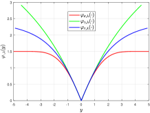
(a)

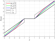
(b)

Figure 1: Curves for (a) generated SIRs and (b) proximity operators with $\lambda=1$, $\sigma=\sqrt{2}\lambda$, $\gamma=\lambda$ and $\tau={\sqrt{3}}\lambda/{2}$.

III-B LRMC via Generated SIRs

In this section, we apply the generated SIRs to LRMC, resulting in:

$$\begin{split}&\mathop{\min}\limits_{\boldsymbol{M}}~{}\|{\boldsymbol{M}}\|_{\varphi_{\cdot,\lambda}},~{}\text{s.t.}~{}\boldsymbol{M}_{\Omega}=\boldsymbol{X}_{\Omega}\end{split}$$ (9)

where $\|\boldsymbol{M}\|_{\varphi_{\cdot,\lambda}}=\sum_{i=1}^{r}\varphi_{\cdot,\lambda}{(\boldsymbol{\sigma}_{i})}$, and $\varphi_{\cdot,\lambda}(\cdot)$ can be the generated regularizer $\varphi_{\sigma,\lambda}(\cdot)$, $\varphi_{\gamma,\lambda}(\cdot)$ or $\varphi_{\tau,\lambda}(\cdot)$. Problem (9) can be converted into the following equivalent form:

$$\begin{split}&\mathop{\min}\limits_{\boldsymbol{M},\boldsymbol{E}}~{}\|\boldsymbol{M}\|_{\varphi_{\cdot,\lambda}}~{}\text{s.t.}~{}\boldsymbol{X}=\boldsymbol{M}+\boldsymbol{E},~{}\boldsymbol{X}_{\Omega^{c}}=0,~{}\boldsymbol{E}_{\Omega}=0\end{split}$$ (10)

which can be solved by the ADMM, and its augmented Lagrangian function is:

$$\begin{split}\mathcal{L}^{\prime}_{\rho}(\boldsymbol{M},\boldsymbol{E},\boldsymbol{\Lambda}):=&\|\boldsymbol{M}\|_{\varphi_{\cdot,\lambda}}+\left<\boldsymbol{\Lambda},\boldsymbol{X}-\boldsymbol{M}-\boldsymbol{E}\right>\\ &+\frac{\rho}{2}\left\|\boldsymbol{X}-\boldsymbol{M}-\boldsymbol{E}\right\|_{F}^{2}\end{split}$$ (11)

which is equal to:

$$\begin{split}\mathcal{L}_{\rho}(\boldsymbol{M},\boldsymbol{E},\boldsymbol{\Lambda}):=&1/\rho\|\boldsymbol{M}\|_{\varphi_{\cdot,\lambda}}+\frac{1}{2}\left\|\boldsymbol{X}-\boldsymbol{M}-\boldsymbol{E}\right\|_{F}^{2}\\ &+1/\rho\left<\boldsymbol{\Lambda},\boldsymbol{X}-\boldsymbol{M}-\boldsymbol{E}\right>\end{split}$$ (12)

where $\boldsymbol{\Lambda}$ is the Lagrange multiplier matrix and $\rho>0$ is the penalty parameter. The variables $\boldsymbol{M},\boldsymbol{E}$ and $\boldsymbol{\Lambda}$ are updated at the $(k+1)$th iteration as follows:

$Update~{}of$ $\boldsymbol{M}$: Given $\boldsymbol{E}^{k}$, $\boldsymbol{\Lambda}^{k}$ and $\rho^{k}$, the estimated matrix $\boldsymbol{M}$ is obtained by:

$${\rm arg}\mathop{\min}\limits_{\boldsymbol{M}}1/\rho^{k}\|\boldsymbol{M}\|_{\varphi_{\cdot,1/\rho^{k}}}+\frac{1}{2}\left\|\boldsymbol{D}^{k}-\boldsymbol{M}\right\|_{F}^{2},~{}\boldsymbol{D}^{k}=\boldsymbol{X}-\boldsymbol{E}^{k}+\frac{\boldsymbol{\Lambda}^{k}}{\rho^{k}}$$ (13)

If $\boldsymbol{D}^{k}=\boldsymbol{U}^{k}\Sigma^{k}\boldsymbol{V}^{k}$ is the singular value decomposition (SVD) of $\boldsymbol{D}^{k}$, then the optimal solution to (13) according to Theorem 1 in [11] is:

$$\boldsymbol{M}^{k+1}=\boldsymbol{U}^{k}P_{\varphi_{\cdot,1/\rho^{k}}}(\boldsymbol{\Sigma}^{k})\boldsymbol{V}^{k}$$ (14)

$Update~{}of$ $\boldsymbol{E}$: Given $\boldsymbol{M}^{k+1}$, $\boldsymbol{\Lambda}^{k}$ and $\rho^{k}$, $\boldsymbol{E}^{k+1}$ is updated by solving:

$${\rm arg}\mathop{\min}\limits_{\boldsymbol{E}_{\Omega^{c}}}\frac{1}{2}\left\|\boldsymbol{X}_{\Omega^{c}}-\boldsymbol{M}_{\Omega^{c}}^{k+1}+\frac{\boldsymbol{\Lambda}_{\Omega^{c}}^{k}}{\rho^{k}}-\boldsymbol{E}_{\Omega^{c}}\right\|_{F}^{2}$$ (15)

with the optimal solution:

$$\boldsymbol{E}_{\Omega^{c}}^{k+1}=\frac{\boldsymbol{\Lambda}_{\Omega^{c}}^{k}}{\rho^{k}}-\boldsymbol{M}_{\Omega^{c}}^{k+1}$$ (16)

Algorithm 1 MC via SIR

0:  $\boldsymbol{X}_{\Omega}$, $\Omega$, $\mu=1.05$, $\xi=10^{-7}$ and $I_{m}=1000$

  Initialize: $\boldsymbol{E}^{0}=\boldsymbol{0}$, $\boldsymbol{\Lambda}^{0}=\boldsymbol{0}$, and $k=0$.

  while $rel_{E}^{k}>\xi$ and $k\leq I_{m}$ do

      Update $\boldsymbol{M}^{k+1}$ via (14)

      Update $\boldsymbol{E}^{k+1}$ via (16)

      Update $\boldsymbol{\Lambda}^{k+1}=\boldsymbol{\Lambda}^{k}+\rho^{k}\left(\boldsymbol{X}-\boldsymbol{M}^{k+1}-\boldsymbol{E}^{k+1}\right)$

      Update $\rho^{k+1}=\mu\rho^{k}$

      $k\leftarrow k+1$

  end while

  $\boldsymbol{M}=\boldsymbol{M}^{k}$.

The steps of the proposed algorithm are summarized in Algorithm 1. It is worth noting that the updates of $\boldsymbol{\Lambda}$ and $\rho$ are only provided in Algorithm 1 due to page limit. When the generated regularizers $\varphi_{\sigma,\lambda}(\cdot)$, $\varphi_{\gamma,\lambda}(\cdot)$ are $\varphi_{\tau,\lambda}(\cdot)$ are adopted in (9), we refer the corresponding algorithm to as MC-HOW, MC-HOC and MC-HOG, respectively. We terminate Algorithm 1 until the relative error $rel_{E}^{k}=\|\boldsymbol{X}-\boldsymbol{M}^{k}-\boldsymbol{S}^{k}\|_{F}/\|\boldsymbol{X}\|_{F}\leq\xi$ or the iteration number reaches the maximum allowable number $I_{m}$. Besides, the SVD computation with complexity of $\mathcal{O}(\min(m,n)mn)$ is involved per iteration. Furthermore, the convergence analysis of Algorithm 1 is provided in Proposition 2, and its proof is similar to the proof of Theorem 3 in [14], thus we omit it due to page limit.

Proposition 2.

The sequence $\{\boldsymbol{M}^{k},\boldsymbol{E}^{k},\boldsymbol{\Lambda}^{k}\}$ generated in Algorithm 1 satisfies:

• The generated sequences $\{\boldsymbol{M}^{k},\boldsymbol{E}^{k},\boldsymbol{\Lambda}^{k}\}$ are bounded.

• $\lim_{k\to\infty}\left\|\boldsymbol{M}^{k+1}-\boldsymbol{M}^{k}\right\|_{F}^{2}=0$
  $\lim_{k\to\infty}\left\|\boldsymbol{X}-\boldsymbol{M}^{k+1}-\boldsymbol{E}^{k+1}\right\|_{F}^{2}=0$.

IV Experimental Results

We compare our algorithms with the competing approaches, including NNM [24], IRNN-$\ell_{p}$ ($p=0.5$) [9] and IRNN-SCAD [10]. All numerical simulations are conducted using a computer with 3.0 GHz CPU and 16 GB memory.

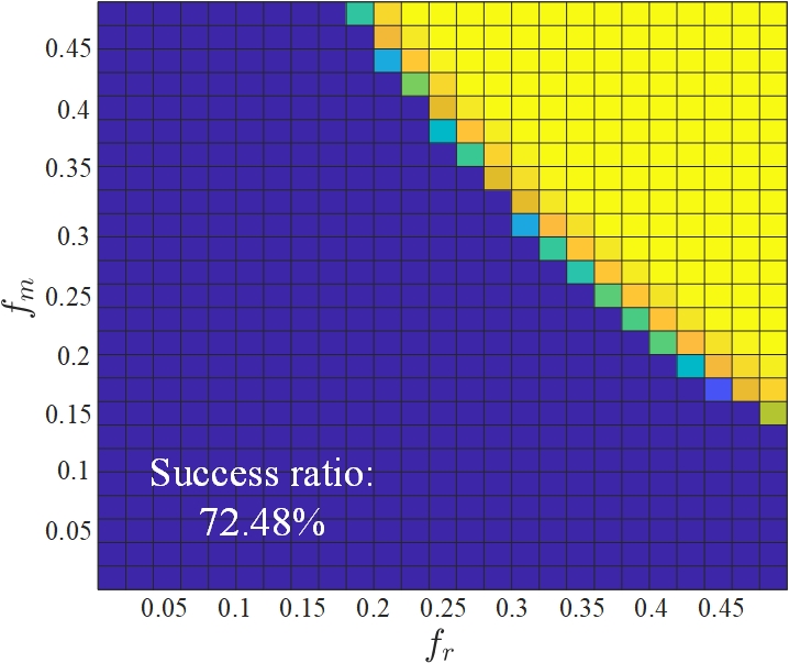
NNM

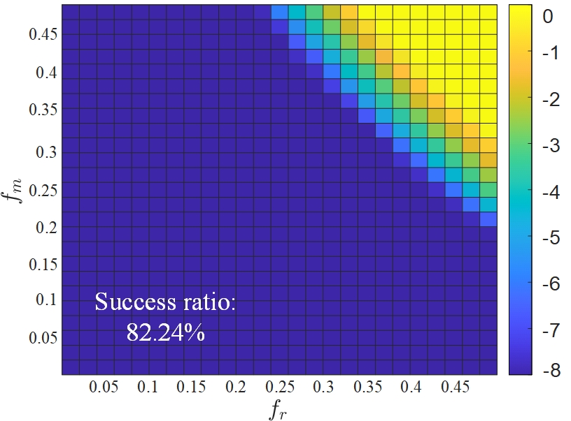
IRNN-$\ell_{p}~{}(p=0.5)$

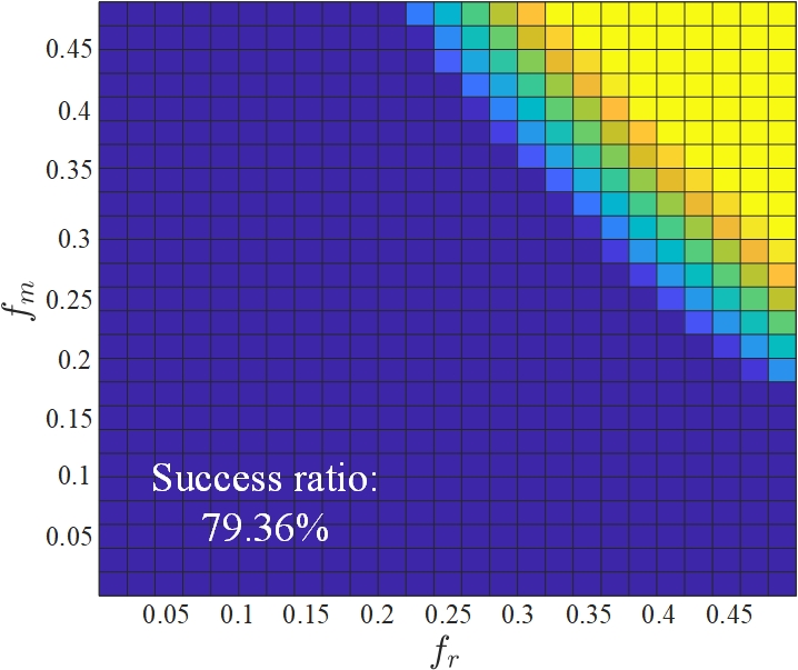
IRNN-SCAD

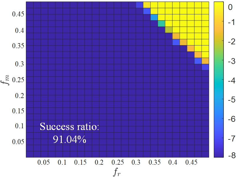
MC-HOW

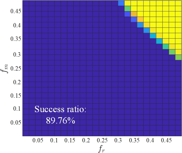
MC-HOC

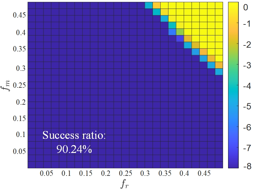
MC-HOG

Figure 2: Algorithm phase transition diagrams with different fractions of full rank and missing entries $\{f_{r},f_{m}\}$.

A rank-$r$ matrix $\boldsymbol{X}=\boldsymbol{U}\boldsymbol{V}$ is first generated, where the entries of $\boldsymbol{U}\in\mathbb{R}^{m\times r}$ and $\boldsymbol{V}\in\mathbb{R}^{r\times n}$ are sampled from the standard Gaussian distribution. In this study, $r=f_{r}\times n$ where $f_{r}$ is the fraction of full rank. Besides, we randomly remove $f_{m}\times m\times n$ entries from $\boldsymbol{X}$, where $f_{m}$ is the fraction of missing entries, to yield the incomplete matrix $\boldsymbol{X}_{\Omega}$. Furthermore, root mean square error (RMSE) defined as ${\rm RMSE}={\|\boldsymbol{X}-\boldsymbol{M}\|_{F}}/{\sqrt{mn}}$ is adopted to measure the recovery performance. In our experiments, $m=300$, $n=200$, $f_{m}$ and $f_{r}$ range from $0.01$ to $0.05$ with a step size of $0.02$. All methods are evaluated by the RMSE based on $100$ independent runs. Fig. 2 shows the log-scale RMSE with different $\{p_{r},p_{s}\}$ values. It is seen that compared with the convex NNM, the nonconvex rank surrogates can recover more cases, and MC-HOW yields the biggest success area. Here, if RMSE $<10^{-3}$, we consider that is a success recovery.

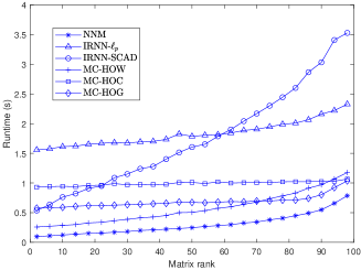
Figure 3: Runtime versus matrix rank.

On the other hand, the runtime (in seconds) for all techniques is investigated under different matrix ranks. Fig. 3 plots runtime versus matrix rank with $f_{m}=0.1$. We see that the runtime of our approaches is less than that of IRNN-$\ell_{p}$ because our regularizers have closed-form proximity operators. Nevertheless, NNM is the most computationally efficient since the proximity operator of the $\ell_{1}$-norm has a simpler expression than those of our SIRs.

V Conclusion

In this paper, we devise a framework to generate SIRs with closed-form proximity operators. We analyze that the Moreau envelope of our regularizers is a convex problem although the regularizers may be nonconvex, and provide the corresponding closed-form solution. Besides, it is proved that the bias generated by our SIRs is less than that by the $\ell_{1}$-norm under certain conditions. Then, we employ our SIRs as nonconvex rank surrogates for LRMC, and algorithms based on the ADMM are developed. Finally, extensive numerical experiments are conducted to demonstrate that the developed algorithms can achieve better recovery under different matrix ranks and missing ratios.

References

- [1] M. A. Davenport and J. Romberg, “An overview of low-rank matrix recovery from incomplete observations,” IEEE J. Sel. Topics Signal Process., vol. 10, no. 4, pp. 608–622, Jun. 2016.
- [2] Z.-Y. Wang, X. P. Li, H. C. So and A. M. Zoubir, “Adaptive rank-one matrix completion using sum of outer products.” IEEE Trans. Circuits Syst. Video Technol., Mar. 2023. Early Access.
- [3] Z.-Y. Wang, X. P. Li and H. C. So, “Robust matrix completion based on factorization and truncated-quadratic loss function,” IEEE Trans. Circuits Syst. Video Technol., vol. 33, no. 9, pp. 1521-1534, Apr. 2023.
- [4] W.-J. Zeng and H. C. So, “Outlier-robust matrix completion via -minimization,” IEEE Trans. Signal Process., vol. 66, no. 5, pp. 1125–1140, Mar. 2018.
- [5] Y. Shen, Z. Wen, and Y. Zhang, “Augmented Lagrangian alternating direction method for matrix separation based on low-rank factorization,” Optimization Methods Softw., vol. 29, no. 2, pp. 239–263, 2014.
- [6] T. Zhou and D. Tao, “Greedy bilateral sketch, completion & smoothing,” in Proc. Int. Conf. Artif. Intell. Statist., Scottsdale, USA, Apr. 2013, pp. 650–658.
- [7] E. J. Candès, and B. Recht, “Exact matrix completion via convex optimization,” Found. Comut. Math., vol. 9, no. 6, pp. 717, Dec. 2009.
- [8] J.-F. Cai, E. J. Candès, and Z. Shen, “A singular value thresholding algorithm for matrix completion,” SIAM J. Opt., vol. 20, no. 4, pp. 1956–1982, Mar. 2010.
- [9] C. Lu, J. Tang, S. Yan, and Z. Lin, “Nonconvex nonsmooth low rank minimization via iteratively reweighted nuclear norm,” IEEE Trans. Image Process., vol. 25, no. 2, pp. 829–839, Feb. 2016.
- [10] C. Lu, J. Tang, S. Yan, and Z. Lin, “Generalized nonconvex nonsmooth low-rank minimization,” in Proc. IEEE Conf. Comput. Vis. Pattern Recog., Silver Spring, MD, USA, Jun. 2014, pp. 4130–4137.
- [11] C. Lu, C. Zhu, C. Xu, S. Yan, and Z. Lin, “Generalized singular value thresholding,” in Proc. AAAI Conf. Artif. Intell., Texas, USA, Jan. 2015, pp. 1805–1811.
- [12] A. Parekh and I. W. Selesnick, “Enhanced low-rank matrix approximation,” IEEE Signal Process. Lett., vol. 23, no. 4, pp. 493–497, Apr. 2016.
- [13] F. Nie, Z. Hu, and X. Li, “Matrix completion based on non-convex low-rank approximation,” IEEE Trans. Image Process., vol. 28, no. 5, pp. 2378–2388, May 2019.
- [14] S. Gu, Q. Xie, D. Meng, W. Zuo, X. Feng, and L. Zhang, “Weighted nuclear norm minimization and its applications to low level vision,” Int. J. Comput. Vis., vol. 121, no. 2, pp. 183–208, Jan. 2017.
- [15] S. Gu, L. Zhang, W. Zuo, and X. Feng, “Weighted nuclear norm minimization with application to image denoising,” in Proc. IEEE Conf. Comput. Vis. Pattern Recognit., Silver Spring, MD, USA, Jun. 2014, pp. 2862–2869.
- [16] M. Nikolova and M. K. Ng, “Analysis of half-quadratic minimization methods for signal and image recovery,” SIAM J. Sci. Comput., vol. 27, no. 3, pp. 937–966, Jan. 2005.
- [17] R. T. Rockafellar and R. J. B. Wets, Variational Analysis, 2nd ed. Berlin, Germany: Springer, 2004.
- [18] F. D. Mandanas and C. L. Kotropoulos, “Robust multidimensional scaling using a maximum correntropy criterion,” IEEE Trans. Signal Process., vol. 65, no. 4, pp. 919–932, Feb. 2017.
- [19] Z.-Y. Wang, H. C. So and A. M. Zoubir, “Robust low-rank matrix recovery via hybrid ordinary-Welsch function.” IEEE Trans. Signal Process., vol. 71, pp. 2548-2563, Jul. 2023.
- [20] R. He, T. Tan, and L. Wang, “Robust recovery of corrupted low-rank matrix by implicit regularizers,” IEEE Trans. Pattern Anal. Mach. Intell., vol. 36, no. 4, pp. 770–783, Apr. 2014.
- [21] R. Chartrand, “Nonconvex splitting for regularized low-rank + sparse decomposition,” IEEE Trans. Signal Process., vol. 60, no. 11, pp. 5810–5819, Nov. 2012.
- [22] P. Combettes and V. Wajs, “Signal recovery by proximal forward-backward splitting,” SIAM J. Multiscale Model. Simul., vol. 4, pp. 1168–1200, 2005.
- [23] F. Shang, J. Cheng, Y. Liu, Z. Luo, and Z. Lin, “Bilinear factor matrix norm minimization for robust PCA: Algorithms and applications,” IEEE Trans. Pattern Anal. Mach. Intell., vol. 40, no. 9, pp. 2066–2080, Sep. 2018.
- [24] Z. Lin, M. Chen, and Y. Ma, “The augmented Lagrange multiplier method for exact recovery of corrupted low-rank matrices,” 2010. [Online]. Available: arXiv:1009.5055.