Coulomb interaction-driven entanglement of electrons on helium

Abstract

The generation and evolution of entanglement in many-body systems is an active area of research that spans multiple fields, from quantum information science to the simulation of quantum many-body systems encountered in condensed matter, subatomic physics, and quantum chemistry. Motivated by recent experiments exploring quantum information processing systems with electrons trapped above the surface of cryogenic noble gas substrates, we theoretically investigate the generation of motional entanglement between two electrons via their unscreened Coulomb interaction. The model system consists of two electrons confined in separate electrostatic traps which establish microwave-frequency quantized states of their motion. We compute the motional energy spectra of the electrons, as well as their entanglement, by diagonalizing the model Hamiltonian with respect to a single-particle Hartree product basis. We also compare our results with the predictions of an effective Hamiltonian. The computational procedure outlined here can be employed for device design and guidance of experimental implementations. In particular, the theoretical tools developed here can be used for fine tuning and optimization of control parameters in future experiments with electrons trapped above the surface of superfluid helium or solid neon.

I Introduction

Entanglement is the fundamental characteristic that distinguishes interacting quantum many-body systems from their classical counterparts. The study of entanglement in precisely engineered quantum systems with countably many degrees of freedom is at the forefront of modern physics, and it is a key resource in quantum information science (QIS). This is particularly true in the development of two-qubit logic for quantum computations, which has been demonstrated in a wide variety of physical systems used in present-day quantum computing, including superconducting circuits [1, 2], trapped ions [3, 4], semiconductor quantum dots [5, 6, 7, 8], color-center defects in diamond [9, 10, 11], and neutral atoms in optical lattices [12, 13]. Investigating the generation and evolution of entanglement in quantum many-body systems is also important for quantum simulations [14, 15, 16, 17], having the potential to advance the fundamental understanding of dense nuclear matter or high-energy physics [18, 19, 20, 21, 22], correlated electron systems [23, 24, 25], and quantum chemistry [26, 27, 28]. Quantum simulators based on natural qubits such as atoms [29, 30, 31], ions [32, 33] and photons [34] are particularly appealing since these systems are highly programmable, controllable and replicable [35]. Additionally, in these systems the coupling to decohering environmental degrees of freedom is minimal, allowing for a tight feedback between experiments and theory.

Trapped electron systems represent a novel approach to investigating the generation of entanglement, sharing many features with platforms based on other natural qubit systems. Recent experimental efforts have investigated the feasibility of trapped electron qubits using ion trap techniques [36, 37]. In fact, the naturally quantized motion of electrons trapped in vacuum above the surface of superfluid helium was one of the earliest theoretical proposals for building a large-scale analog quantum computer [38]. The surface of the superfluid functions as a pristine substrate [39], shielding the electrons from deleterious sources of noise at the device layer beneath helium. Since this initial proposal, a number of theoretical ideas have been put forward to create both charge [40, 41, 42, 43, 44] and spin [45, 42, 46, 44, 47] qubits based on these trapped electrons. Additionally a wide variety of experimental work, directed at realizing these electronic qubits, has been performed to leverage advances in nano-fabrication techniques for precision trapping and control of electrons on helium in confined geometries [48, 49, 50, 51, 52], mesoscopic devices [53, 54, 55], circuit quantum electrodynamic architectures [56, 57], and surface acoustic wave devices [58]. Single-electron trapping and detection have been experimentally achieved [53, 59, 57], as well as extremely high-fidelity electron transfer along gated arrays fabricated using standard CMOS processes [60]. Similarly, electrons trapped above the surface of solidified noble gases offer an alternative trapped electron qubit; electrons trapped in vacuum above the surface of solid neon have recently been experimentally demonstrated as a novel natural charge qubit [61] with high coherence [62].

In aggregate, these technological advances have opened the door to exploring the generation and evolution of entanglement in systems based on trapped electrons. Here we present a model system for investigating the entanglement between the microwave-frequency motional states of two electrons trapped in vacuum above the surface of a layer of superfluid helium. The electrons are confined laterally by applying voltages to electrodes in a substrate beneath the condensed helium layer. These voltages are tuned to set up electrostatic traps on the helium surface to control the relative position of the electrons and quantize their in-plane motional states in the GHz-frequency range. We utilize the full configuration interaction (CI for short in this work) method [63] for distinguishable particles to compute the quantized motional excitations of the system, as well as the entanglement between the electrons generated by Coulomb interaction. These numerical studies are in turn used to optimize the electrode voltages to maximise the entanglement. We also present an effective theoretical model of the two-electron system, as a useful tool to analyze the underlying coupling mechanism between the electrons. Given the exact solution provided by the CI calculations, we discuss the limitations of the approximations of this effective model. Our work can be used to provide feedback to future experimental realizations in which, ultimately, control and readout of charged qubit states can be achieved, via integration of microwave resonators [42, 57, 61, 62] using standard techniques based on circuit quantum electrodynamics (cQED) [64].

In section II we present a schematic micro-device that allows for controlled Coulomb-driven entanglement between two electrons. We also describe a numerical procedure to find the optimal parameters for this device to function as a two-qubit quantum computer. Section III contains our main results, with detailed discussion of the system properties and comparison to an effective model Hamiltonian. The final section contains conclusions, perspectives, and outlook for future work. Additional details are presented in various appendices.

II Device and Theory

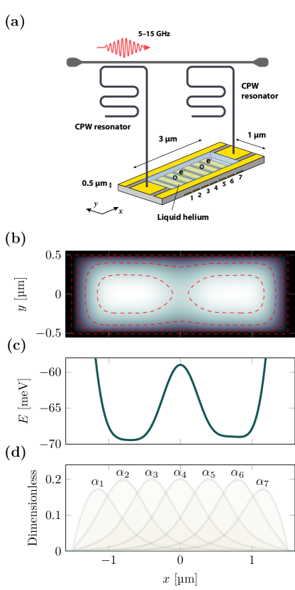
Figure 1: (a) Schematic micro-device, in which two electrons are trapped on the surface of a liquid helium basin in a double-well potential created by electrodes 1–7. Control and readout of the quantized motion is provided by two superconducting resonators, dispersively coupled to the in-plane motional states of the electrons. (b) Example configuration for the full two-dimensional electrostatic potential in the device, which realizes two separate wells. Brighter colors represent a stronger potential given in arbitrary units. (c) One-dimensional linecut of the potential in (b) along $y=0$. (d) One-dimensional coupling constants from each individual electrode beneath the helium layer along $y=0$. These coupling constants give rise to the total potential as given by Eq. (1).

Electrons placed in vacuum above a layer of liquid helium are drawn toward the liquid by an attractive force produced by positive image charges in the dielectric liquid. However, the electrons are prevented from entering the liquid by a large ($\sim$1 eV) Pauli barrier at the liquid-vacuum interface [65, 66]. The balancing of these two effects creates a ladder of Rydberg-like states for the vertical motion of the electrons, and at low temperatures the electrons are naturally initialized into the ground state of this motion approximately $11\text{\,}\mathrm{n}\mathrm{m}$ above the helium surface [67, 68]. The electrons experience only a weak interaction with their environment, which is mainly governed by interactions with thermally excited ripplons (quantized capillary waves on the helium surface) and phonons in the bulk of the liquid [69]. Based on these interactions, theory predicts long coherence times of both the electron spin and motional degrees of freedom [40, 70, 46]. The electron in-plane motion can be further localized on length scales approaching an electron separation of around $1$ µm through the integration of micro-devices that provide lateral confinement [71, 72, 57]. Devices of this type have been used to demonstrate single electron trapping [73, 57, 74], and to investigate the two-dimensional crystalline electronic phase known as the Wigner solid [72, 75], which arises from the largely unscreened Coulomb repulsion between the electrons. As explored in this work, this strong electron-electron interaction can also in principle be utilized to couple the quantum motion of electrons and create entanglement between electron charge qubits, in analogy to a Cirac-Zoller entangling gate [76].

II.1 Device design

A schematic micro-device for investigating the Coulomb-driven entanglement of the in-plane motional states of two electrons on helium is sketched in Fig. 1(a). Here we consider a $3\times 1$ µm² size microchannel structure with a depth of 0.5 µm, filled with superfluid helium via capillary action [77]. Once the device is filled, thermionic emission from a tungsten filament located above the helium surface can be used to generate electrons, which are then naturally trapped above the liquid surface. We note that trapping one or two electrons also requires controlled loading and unloading of electrons into the trap region from a larger reservoir area where electrons are stored (not shown in Fig. 1(a)). This type of electron manipulation is quite standard and has been experimentally demonstrated in multiple devices, see for example Refs. [78, 57]. For the purpose of the current theoretical study, we consider a simple array of electrodes that allow for the investigation of entanglement between two electrons, which we assume have already been loaded successfully into the device. The rectangular device geometry and dimensions were chosen to create an in-plane motional quantization axis along the $x$-direction, with energy gaps in the frequency range of $5$–$15$ GHz. These states are decoupled from motional states along the $y$-direction at significantly higher frequency, which we will ignore for the purposes of this one-dimensional study. Voltages applied to seven $200$ nm-wide electrodes spaced by $200$ nm beneath the helium layer provide the degrees of freedom needed to form an electrostatic double-well potential for the two electrons as shown in Figs. 1(b,c). The electrostatic potential in the trap region is given

$$\varphi(x,y)=\sum_{i=1}^{7}\alpha_{i}(x,y)V_{i},$$ (1)

where $\alpha_{i}=C_{i}/C_{\Sigma}$ is the relative contribution to the potential defined by the capacitance between a region of space at position $(x,y)$ on the helium surface and the corresponding electrode. The total capacitance is $C_{\Sigma}=\sum_{i}C_{i}$, and $V_{i}$ is the voltage applied to the $i^{\textrm{th}}$ electrode, which can be adjusted to create particular trapping potential configurations. We note that the top electrodes at the helium surface are held at ground potential. The coupling constants $\alpha_{i}(x,y)$ are calculated by solving the Laplace equation for the electrostatic potential numerically, using standard finite-element modeling techniques (see Fig. 1(d)). The double-well trap is achieved by applying a negative voltage to the central electrode (electrode 4 in Fig. 1(a)) and positive voltages to the other electrodes. Particular choices of applied voltages will be described further in Section III, where we also discuss how this setup allows us to adjust the electron motional frequencies over a broad range, enabling thereby the generation of entanglement between the two electrons at certain conditions.

Coherent control and readout of the electron motional states in this type of micro-device is based on coupling the electron motional states to microwave frequency photons in superconducting resonators, see Fig. 1(a), with a coupling $g_{\mathrm{RF}}/2\pi=\langle 1|\mathbf{d}\cdot\mathbf{E}|0\rangle=ef_{\mathrm{RF}}\partial\alpha_{\mathrm{RF}}/\partial x\sqrt{Z_{\mathrm{RF}}/m_{e}\omega_{\text{e}}}$. In this expression $\mathbf{d}$ is the dipole moment of the oscillating electron along the $x$-axis, $\mathbf{E}=\partial\alpha_{\mathrm{RF}}/\partial x\cdot V_{\mathrm{zpf}}\hat{\mathbf{x}}$ is the electric field created by the resonator at the position of the electron, $e$ and $m_{e}$ are the electron charge and mass respectively, $\alpha_{\mathrm{RF}}$ is the coupling constant for the resonator electrode, $V_{\mathrm{zpf}}$ is the voltage amplitude of zero point fluctuations in the resonator, $f_{\mathrm{RF}}$ and $Z_{\mathrm{RF}}$ are resonator frequency and impedance, and $\omega_{\text{e}}$ is the electron motional frequency along the $x$-axis. For typical values of $\partial\alpha_{\mathrm{RF}}/\partial x=0.5\times 10^{6}$ m^-1, $Z_{\mathrm{RF}}=50$ $\Omega$, $f_{\mathrm{RF}}=7$ GHz and $\omega_{\text{e}}/2\pi=5$ GHz, we find $g_{\mathrm{RF}}/2\pi\simeq 12$ MHz.

At low temperatures, the decay of energy from the electrons-on-helium system occurs due to its interaction with helium surface ripplons and bulk phonons (see for example [40, 46]). The total rate of decoherence due to these processes has been estimated to be approximately $\Gamma/2\pi=3\times 10^{4}$ Hz [40], allowing the realization of the strong coupling regime ($g_{\mathrm{RF}}\gg\Gamma$) between the microwave photons and the electron motional states.

In this device, the two electrons are coupled individually to two superconducting coplanar waveguide (CPW) $\lambda/4$-resonators, each having a different resonant frequency. The crosstalk coupling between an electron and the other electron’s resonator is several times smaller than the direct coupling to its own resonator, so we will ignore this in our analysis. It should be noted that this classical crosstalk can ultimately limit the fidelity of gate operations, but it can be mitigated by applying appropriate compensation tones [79]. In the dispersive regime of cQED, in which $g_{\mathrm{RF}}/|\omega_{\text{e}}-\omega_{\mathrm{RF}}|\ll 1$, the frequency of the resonator is sensitive to the state of the electronic motion, which can be detected by measuring the transmitted microwave signals through the CPW feedline connected to the resonators [42, 57, 64].

II.2 Model Hamiltonian

Our model Hamiltonian describes two electrons trapped in a double-well potential set up by seven electrodes as given in Eq. (1), but we restrict our calculations along the $x$-direction only. The interaction between the electrons is given by a Coulomb term which gives rise to their correlated motion. The full Hamiltonian for the system, in dimensionless units, is then given by

$$\hat{H}=\sum_{i=1}^{2}\quantity(-\frac{1}{2}\derivative[2]{x_{i}}+v(x_{i}))+u(x_{1},x_{2}),$$ (2)

where $v(x)=-e\varphi(x)/E_{\mathrm{d}}$ is the trap potential. Here, $\varphi(x)=\varphi(x,0)$ is the electrostatic trap potential given in Eq. (1), and $E_{\mathrm{d}}=\hbar^{2}/m_{\mathrm{e}}x_{0}^{2}$ is our energy unit ($\hbar$ is the reduced Planck constant). The value $x_{0}=123$ nm is our length unit, representing the characteristic inter-electron distance corresponding to a typical electron density of $\simeq 2\times 10^{9}$ cm^-2 in micro-devices [72]. The soft Coulomb interaction is given by

$$u(x_{1},x_{2})=\frac{\kappa}{\sqrt{\quantity(x_{1}-x_{2})^{2}+\epsilon^{2}}},$$ (3)

where $\kappa=e^{2}/(4\pi\varepsilon_{0}E_{\mathrm{d}})=2326$ gives the strength of the Coulomb interaction ($\varepsilon_{0}$ is the vacuum permittivity). We have introduced a shielding parameter $\epsilon=10^{-2}$ to remove the singularity at $x_{1}=x_{2}$ [80]. We note that due to the small distance between the electrons and the underlying electrodes, the Coulomb interaction will be reduced due to screening effects. However in our analysis we consider an unscreened Coulomb interaction, which sets an upper bound for the interaction strength between the two electrons.

As long as the double-well potential $v(x)$ is sufficiently deep, there will be no tunneling through the barrier between the wells for the bound electron states.

This encourages us to split it into two separate potential wells. Denoting the position of the barrier maximum by $x_{b}$, we can define

$$\begin{gathered}v^{L}(x)=\begin{cases}v(x),&x<x_{b},\\ v(x_{b}),&x\geq x_{b},\end{cases}\\ v^{R}(x)=\begin{cases}v(x_{b}),&x<x_{b},\\ v(x),&x\geq x_{b},\end{cases}\end{gathered}$$ (4)

with $L$ and $R$ labeling the left and the right wells respectively. We can then express the total double-well potential as the sum $v(x)=v^{L}(x)+v^{R}(x)-v(x_{b})$. Since there is negligible spatial overlap between single-electron states in different wells, we can omit spin and focus on motional product states in which one electron is localized in the left well while the other electron is localized in the right well.

In essence, a sufficiently deep double-well trap allows us to treat the electrons as distinguishable particles, labeled by their position. The one-body Hamiltonian for each electron can then be written as

$$\hat{h}^{A}=-\frac{1}{2}\derivative[2]{x}+v^{A}(x),$$ (5)

with $A\in\quantity{L,R}$, and the two-body Hamiltonian is given by Eq. (2).

Throughout our analysis we will vary the seven electrode voltages $V_{i}$ to adjust the shape of the double-well potential $v(x)$, and hence also the energy spectrum and frequencies of our system. We will refer to each such choice as a well configuration, and the tuning between configurations is what allows us to realize various quantum gates.

II.3 State ansatz

We solve the two-body problem described in the previous section by exact diagonalization of the Hamiltonian in Eq. (2) with respect to a single-particle product basis. The two-body state ansatz we use is

$$\ket*{\Phi_{n}} =\sum_{i=0}^{N^{L}}\sum_{j=0}^{N^{R}}C_{ij,n}\ket*{\phi^{L}_{i}\phi^{R}_{j}}.$$ (6)

Here, $n$ is the index of each two-body energy eigenstate, and $\ket*{\phi^{L}_{i}\phi^{R}_{j}}=\ket*{\phi^{L}_{i}}\otimes\ket*{\phi^{R}_{j}}$ are two-body product states built from two single-particle basis sets $\quantity{\ket*{\phi^{A}_{i}}\mid i=0,\dots,N^{A}}$ (with $A\in\quantity{L,R}$). The above ansatz is analogous to the ansatz of full configuration-interaction (CI) theory, but since our electrons are effectively distinguishable we use separable product states instead of anti-symmetrized Slater determinants in our expansion [63].

The quality of the ansatz in Eq. (6) depends on the choice of single-particle basis states $\ket*{\phi^{A}_{i}}$. Even though we consider only two particles, a large single-particle basis will quickly make the exact diagonalization procedure prohibitively time consuming. This limits us to consider small single-electron basis sets, whose product states span the state space of our two-electron system to a good approximation. One option is to consider the eigenstates of the individual one-body Hamiltonians $\hat{h}^{A}$ defined in Eq. (5). However, this approach neglects all information about interactions and, as a consequence, still demands a significant number of basis states to accurately capture the physics. A more effective approach is to employ the Hartree method (analogous to the Hartree-Fock method, but for distinguishable particles), which incorporates the one-body Hamiltonian with a mean-field contribution from the Coulomb interaction. This method has the advantage of producing single-particle basis sets that can be truncated to only a few states while still capturing the interaction physics of the entangled two-body states within our system.

The construction of the Hartree basis sets $\ket*{\phi^{A}_{i}}$ and derivation of the Hartree method are presented in Appendices A and B. With the single-particle basis sets established, the coefficients $C_{ij,n}$ in Eq. (6) can be calculated to find the full two-body energy eigenstates for each well configuration. This is done through a diagonalization procedure, which is explained in detail in Appendix C.

We should add, as discussed in more detail in appendices A and C, that we also have performed full configuration interaction calculations with an anti-symmetrized wave function basis for the two-electron system. For the system we are investigating, the Hartree ansatz with distinguishable particles gives an excellent approximation to the anti-symmetrized full configuration interaction calculations.

II.4 Entanglement

It is natural to consider the system at hand as bipartite, composed of the two electrons as, ideally, individual subsystems. Such a bipartition comes with the notion of entanglement — the inability to discern the exact state of each subsystem, even though the state of the full system is known. We aim to find certain well configurations for which a subset of the energy eigenstates are entangled, in order to enable the set up of two-qubit gates, see for example the discussions in Refs. [8, 81, 82].

A common entanglement measure for bipartite systems is the von Neumann entropy of a quantum state, defined as

$$S=-\tr\!\quantity(\hat{\rho}\log_{2}(\hat{\rho})),$$ (7)

where $\hat{\rho}$ is the reduced density operator of either subsystem. We use this measure to quantify entanglement and will refer to it simply as the entropy. (See appendix D for calculational details.) In what follows we denote the entanglement entropy of each energy eigenstate $\ket*{\Phi_{n}}$ by $S_{n}$.

The two-body state of the full system can be expanded in any product state basis from the subsystems, such as in (6). While the Hartree basis discussed above provides a succinct picture of the interaction between subsystems, another basis offering a clear picture of the entanglement is the Schmidt basis, found by doing a singular-value decomposition of the coefficient matrix $C_{ij,n}$ as outlined in appendix D. In the Schmidt decomposition of a two-body state, each term involves a product of unique, orthogonal Schmidt states. It follows that the Schmidt states are eigenstates of the reduced density operators of each subsystem. Then, the mixed state of each subsystem can be interpreted as a statistical ensemble of its Schmidt states, and the Schmidt coefficients (the singular values), when squared, give the occupation number of each Schmidt state. Our calculations indicate that the Hartree basis actually serves as an approximate common Schmidt basis for all the two-body energy eigenstates of our system. In addition to the von Neumann entropies $S_{n}$, we therefore map the two-body coefficients $C_{ij,n}$ to provide a clear overview of which products of single-electron states that are involved in each entangled two-body state. For simplicity, we will denote the Hartree product states as

$$\ket*{\phi^{L}_{i}\phi^{R}_{j}}=\ket{ij},$$ (8)

but note that these product states are not to be directly interpreted as computational basis states for quantum computing. We can not do any measurements to collapse the two-electron system into any of these separable states, so they should be interpreted only as an ideal single-particle product basis for describing the two-body states of our system. The states that should be interpreted as computational basis states, are four specific energy eigenstates of configuration I, as defined in section II.5 below.

II.5 Gate operation

We target three specific well configurations that are ideal for operation of one-qubit rotations as well as two-qubit $\sqrt{i\mathrm{SWAP}}$ and CZ gates [83, 81, 84]. Each configuration is defined through specific entanglement entropies of the two-body energy eigenstates.

Configuration I, see also the discussions in the next subsection and Fig. 2, corresponds to the case in which each electron has a distinct transition frequency between its ground and first-excited state. The correlations between the two electrons are then minimal, and the state of the electrons can be controlled and read out independently via their associated resonators. We focus on cases in which the frequency of the left qubit is larger than that of the right qubit, and within the resonator working range of 5–15 GHz. Then the two-body energy eigenstates $\ket*{\Phi_{0}}$, $\ket*{\Phi_{1}}$, $\ket*{\Phi_{2}}$ and $\ket*{\Phi_{4}}$ have maximum overlap with the Hartree product states $\ket*{00}$, $\ket*{01}$, $\ket*{10}$ and $\ket*{11}$, respectively, and we interpret these eigenstates as computational basis states. Due to the minimized correlation, the entanglement entropy is zero for all energy eigenstates of this configuration.

Configuration II is designed to realize the two-qubit $\sqrt{i\mathrm{SWAP}}$ gate. It can be achieved by an avoided crossing of the first and second excited eigenstates, so that they are given by

$$\ket*{\Phi_{1}} =\quantity(\ket*{10}-\ket*{01})/\sqrt{2},$$ (9)

$$\ket*{\Phi_{2}} =\quantity(\ket*{10}+\ket*{01})/\sqrt{2}.$$

All other energy eigenstates must remain product states to ensure that only $\ket*{10}$ and $\ket*{01}$ are coupled. The entropy is then $1$ for the two states $\ket*{\Phi_{1}}$ and $\ket*{\Phi_{2}}$ and zero for the rest. For a further discussion of avoided level crossings in coupled quantum dot systems, see for example Ref. [8].

The presence of higher energy levels gives rise to a different type of correlation between the two electrons in our system. We are particularly interested in a specific type of interaction that enable the realization of a controlled-phase CZ gate [64, 84]. Configuration III realizes the conditions to implement this type of two-qubit gate, which involves a “triple” avoided crossing between the third, fourth and fifth excited eigenstates:

$$\ket*{\Phi_{3}} =\quantity(\ket*{20}-\ket*{02}-\sqrt{2}\ket*{11})/2,$$ (10)

$$\ket*{\Phi_{4}} =\quantity(\ket*{20}+\ket*{02})/\sqrt{2},$$

$$\ket*{\Phi_{5}} =\quantity(\ket*{20}-\ket*{02}+\sqrt{2}\ket*{11})/2.$$

The entropies of these states are $1.5$, $1$ and $1.5$, respectively. In this configuration, too, the remaining energy eigenstates must stay as close to their non-interacting counterparts as possible, with entropy close to zero. To quantify the strength of this two-qubit interaction, we define the $ZZ$ coupling strength [82, 85, 86], see also discussions below, as

$$\zeta=E_{4}-E_{2}-E_{1}+E_{0}.$$ (11)

This quantity measures the shift in transition frequency of one electron when the other electron is excited. The $ZZ$-coupling plays an important role in our analysis since it conveys information about the coupling to higher excited states.

In configurations I and II, $\zeta$ should be as small as possible to minimize phase errors when driving gates. However, in configuration III the action of the shift can be used to alter the phase of the computational basis state $\ket*{\Phi_{4}}$, which generates the CZ gate [81, 85, 84].

Tuning the electrode voltages diabatically between configuration I and configurations II or III, the above-mentioned two-body quantum gates are realizable [81, 84]. We proceed to demonstrate that the necessary well configurations and resulting electron entanglement are achievable through targeted numerical optimization. The remainder of this work is focused on the resulting configurations, and we will leave actual simulations of time-dependent gate operation to future work.

II.6 Configurational search

The three desirable well configurations defined in the previous section can be targeted through numerical optimization methods, with the seven electrode voltages as the variational parameters. To achieve the avoided crossings described above, we can use the fact that the Hartree product basis incorporates much of the Coulomb interaction between the electrons, so that the residual Coulomb interaction term is small. This means that the energy spectrum of the full interacting system should be close to the spectrum of Hartree product states $\ket*{ij}$, with transition energies given by the sum of the corresponding Hartree transition energies $\epsilon^{L}_{i}-\epsilon^{L}_{0}+\epsilon^{R}_{j}-\epsilon^{R}_{0}$ (where $\epsilon^{A}_{i}$ are the eigenvalues of the Hartree states as defined in appendix B). This approximation matches the interacting spectrum well except at the avoided crossings, where the interaction turns what would have been an energy crossing in the non-interacting case into an avoided crossing in the interacting case. In other words, we can look at the Hartree energies of the system and target degenerate Hartree energies to find avoided crossings.

We also target qubit anharmonicities of equal magnitude but opposite sign throughout all three configurations. This was shown to suppress the unwanted $ZZ$-coupling defined in (11) for superconducting qubits [84, 85, 86], and so we investigate if the same principle is applicable to our charge qubits. The anharmonicity of each qubit can again be defined through the Hartree energies, which serve as a non-interacting, single-particle guiding picture throughout this section.

Figure 2: (a) Transition frequencies in the non-interacting picture for configuration I. This configuration corresponds to a detuned system in which all transition energies are distinguishable, and $\Delta_{\mathrm{I}}=\omega^{L}-\omega^{R}>0$, with $\beta^{L}=-\beta^{R}=\Delta_{\mathrm{I}}/2$. (b) Transition frequencies in configuration II. Here the detuning is zero, $\Delta_{\mathrm{II}}=0$, and the two states $\ket*{10}$ and $\ket*{01}$ are degenerate in the absence of interactions. Distinct anharmonicities kept at $\beta^{L}=-\beta^{R}=\Delta_{\mathrm{I}}/2$ separate the higher states from one another. (c) Configuration III is realized when the three states $\ket*{20}$, $\ket*{11}$ and $\ket*{02}$ share the same transition frequency from the ground state. This occurs when $\beta^{L}=-\beta^{R}=-\Delta_{\mathrm{III}}$. The detuning has opposite sign of that in configuration I, $\Delta_{\mathrm{III}}=-\Delta_{\mathrm{I}}/2$.

Figure 2 illustrates the non-interacting energy spectra of the three target configurations. The transition frequency from $\ket*{0}$ to $\ket*{1}$ for subsystem $A\in\quantity{L,R}$ is denoted by $\epsilon^{A}_{1}-\epsilon^{A}_{0}=\omega^{A}$ (with $\hbar=1$). In order to selectively address the ground and first excited energy eigenstates while avoiding population of higher states, the electrostatic potential is intentionally designed to be anharmonic. We define the anharmonicity to be the difference in the excitation energy between $\ket*{0}\to\ket*{1}$ and $\ket*{1}\to\ket*{2}$. Consequently, the transition frequency for $\ket*{0}\to\ket*{2}$ is given by $\epsilon^{A}_{2}-\epsilon^{A}_{0}=2\omega^{A}+\beta^{A}$, where $\beta^{A}$ is the anharmonicity.

The energy of the non-interacting Hartree product state $\ket*{ij}$ is given by $\epsilon_{ij}=\epsilon^{L}_{i}+\epsilon^{R}_{j}$. We refer to the difference in energy between the states $\ket*{10}$ and $\ket*{01}$ as the qubit detuning, and denote it by $\Delta\equiv\omega^{L}-\omega^{R}$. Using the detuning and the anharmonicity we can express the transition frequencies for $\ket*{11}\to\ket*{20}$ and $\ket*{02}\to\ket*{11}$ by $\epsilon_{20}-\epsilon_{11}=\Delta+\beta^{L}$ and $\epsilon_{11}-\epsilon_{02}=\Delta-\beta^{R}$.

Figure 2(a) illustrates the non-interacting energy spectrum for configuration I. In this configuration all transition frequencies are distinct, and we have chosen a detuning of $\Delta_{\mathrm{I}}=\omega^{L}-\omega^{R}>0$ so that the electron in the left well has higher transition frequencies than the electron in the right well. Furthermore, we have set $\beta^{L}=-\beta^{R}=\Delta_{\mathrm{I}}/2$ such that $\Delta+\beta^{L}=\Delta-\beta^{R}>\Delta$, i.e., the energy gaps between $\ket*{20}$ and $\ket*{11}$, and $\ket*{11}$ and $\ket*{02}$ are equally large, and greater than the detuning.

Figure 2(b) shows the target non-interacting energy spectrum for configuration II. In this configuration the single-particle basis states $\ket*{01}$ and $\ket*{10}$ are degenerate, while the higher states $\ket*{20}$, $\ket*{11}$ and $\ket*{02}$ are kept separate from each other. This implies that $\Delta_{\mathrm{II}}=\omega^{L}-\omega^{R}=0$, and we have maintained the anharmonicities at the same values as in configuration I, i.e., $\beta^{L}=-\beta^{R}=\Delta_{\mathrm{I}}/2$.

Finally, Fig. 2(c) shows the target non-interacting energy spectrum for configuration III. In this configuration the higher states $\ket*{20}$, $\ket*{11}$ and $\ket*{02}$ are degenerate, while $\ket*{10}$ and $\ket*{01}$ are distinct. To realize this configuration we require $\Delta+\beta^{L}=\Delta-\beta^{R}=0$, and with $\beta^{L}=-\beta^{R}$ we find $\beta^{L}=-\Delta$. Keeping the anharmonicities of the two wells the same as in configuration I and II, i.e., $\beta^{L}=-\beta^{R}=\Delta_{\mathrm{I}}/2$, leads to $\Delta_{\mathrm{III}}=-\Delta_{\mathrm{I}}/2$.

The residual Coulomb interaction between the electrons splits the degeneracy in energy levels and leads to avoided level crossings, entanglement between the two electrons, and hence the possibility of driving two-qubit gates. The anharmonicities being non-zero, with equal magnitude and opposite sign also ensure that the avoided crossing between the first and second excited states and the triple avoided crossing between the higher states are separated [84, 85].

We note, as indicated in Figs. 2(a,c), that the detunings in configuration I and configuration III have opposite signs. This is not incidental, but has a deliberate purpose; it allows for the realization of configuration II somewhere in the transitional region between configuration I and III, as long as the anharmonicities have a magnitude greater than zero along the same path. This happens because the detuning has to change sign in order to go from configuration I to configuration III, leading to the characteristic level crossing of configuration II when the detuning is zero. Hence, our task simplifies to locating configurations I and III with equal anharmonicities by tuning the electrode voltages. We can then define a parametrization that interpolates between these two configurations, and as long as the anharmonicities do not go to zero, we are guaranteed to get a configuration II somewhere along the parametrization path.

III Results and Discussion

We start this section by summarizing the numerical optimization procedure that was used to locate the above-defined configurations I and III in the parameter space of seven electrode voltages. We then define a parametrization of the voltages and identify the location of configuration II. Thereafter we discuss the properties of each configuration in more detail. Finally, we make an attempt at interpreting our results in terms of a phenomenological model.

III.1 Configurational results

To find the electrode voltages corresponding to configurations I and III, we express the search as an optimization problem by defining cost functions whose minima align with the desired properties for each configuration, as described in section II.6. Each cost function was minimized by evaluating its gradient with respect to the voltages. The optimization of the cost functions was done using standard gradient descent methods with the so-called ADAM algorithm [87] for the gradient updates. As is common in the optimization of multi-parameter functions, we found that our cost functions often exhibit several local minima, a feature which makes our solution dependent on the initial guess for the voltages. Because of this, our approach involved manually adjusting the voltages to obtain an initial well configuration resembling a double-well trap with features close to the desired properties, and then running the optimization search. Appendix F provides an in-depth discussion of the full optimization process, including specific expressions for the cost functions.

For configuration I, this procedure successfully achieves distinct transition frequencies of each well, within the resonator working range of 5–15 GHz. We also target anharmonicities with equal magnitude and opposite signs to suppress $ZZ$ crosstalk in higher energy states as discussed in section II.6. However, an arbitrary choice of transition frequencies and anharmonicities does not necessarily result in an appropriate well configuration. By performing the optimization process for a range of possible candidates, we ended up targeting the specific transition frequency of $\omega^{L}/2\pi=$11\text{\,}\mathrm{GHz}$$ between the two lowest energy levels in the left well, and a transition frequency of $\omega^{R}/2\pi=$9\text{\,}\mathrm{GHz}$$ in the right well. This corresponds to a detuning of $\Delta_{\mathrm{I}}/2\pi=(\omega^{L}-\omega^{R})/2\pi=$2\text{\,}\mathrm{GHz}$$. At the same time, anharmonicities of $\beta^{L}/2\pi=-\beta^{R}/2\pi=(\Delta_{\mathrm{I}}/2)/2\pi=$1\text{\,}\mathrm{GHz}$$ were targeted. Optimization of the cost function based on these target values (Eq. (F) in Appendix F) yields properties that are very close to the desired ones. The two-body energies of the resulting configuration are $E_{1}/2\pi=$8.99\text{\,}\mathrm{GHz}$$ and $E_{2}/2\pi=$11.01\text{\,}\mathrm{GHz}$$ relative to the ground state, and the anharmonicities are equal to the targeted values of $\pm 1\text{\,}\mathrm{GHz}$ to three decimal places.

For configuration III, we achieve a triple degeneracy point between the computational basis state $\ket{11}$ and the states $\ket{20}$ and $\ket{02}$. Here we construct a cost function targeting the entropies of the energy eigenstates $\ket{\Phi_{3}}$, $\ket{\Phi_{4}}$ and $\ket{\Phi_{5}}$ to be $1.5$, $1.0$ and $1.5$ respectively, while keeping the entropies of all other eigenstates small. In addition, we target the detuning $\Delta_{\mathrm{III}}/2\pi$ to be $-1\text{\,}\mathrm{GHz}$ and the same anharmonicities as for configuration I, $\beta^{L}/2\pi=-\beta^{R}/2\pi=$1\text{\,}\mathrm{GHz}$$. As discussed earlier, this guarantees the presence of configuration II for a certain set of voltages in the transition from configuration I to configuration III. We use the set of voltages obtained for configuration I as an initial guess for the optimization of this cost function (Eq. (F) in Appendix F). This optimization results in two-body energies $E_{3}/2\pi=$27.24\text{\,}\mathrm{GHz}$$, $E_{4}/2\pi=$27.42\text{\,}\mathrm{GHz}$$ and $E_{5}/2\pi=$27.61\text{\,}\mathrm{GHz}$$ relative to the ground state, with entropies of 1.50, 1.00 and 1.49, respectively.

To visualize properties of the configurations and the tuning between them, we express the seven electrode voltages with one configuration parameter $\lambda$, through a linear parametrization

$${\bf\it V}(\lambda)=(1-\lambda){\bf\it V}_{\mathrm{I}}+\lambda{\bf\it V}_{\mathrm{III}}.$$ (12)

Here, ${\bf\it V}_{\mathrm{I}}$ and ${\bf\it V}_{\mathrm{III}}$ are vectors with the optimized voltages for configurations I and III. By construction, configuration I then corresponds to $\lambda=0$ while configuration III corresponds to $\lambda=1$. Explicit values of the voltages for each optimized configuration are provided in table 1 in Appendix G.

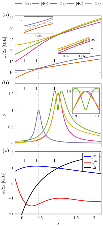
Figure 3: (a) Transition frequencies from the ground state of the five lowest excited energy eigenstates, as functions of the configurational parameter $\lambda$. Solid lines correspond to the transition energies of the full Hamiltonian. In the insets we have included thin dashed lines for the transition energies of the non-interacting Hartree product states. (b) Von Neumann entropies of the same five eigenstates as functions of the configurational parameter $\lambda$. The entropy is calculated with the binary (base-2) logarithm. (c) Anharmonicites of the left ($\beta^{L}$) and right ($\beta^{R}$) wells as functions of the configurational parameter $\lambda$, as well as the detuning $\Delta=\omega^{R}-\omega^{L}$ between the two wells. Marked in all subfigures are configurations I, II and III at their respective $\lambda$ values of $0$, $0.46$ and $1$.

Figure 3 shows CI results for the two-body energy spectrum for the five lowest excited states, the corresponding entanglement entropies, as well as the anharmonicities and detuning of the wells as a function of the configurational parameter $\lambda$. Two avoided crossings are clearly observed in the spectrum in Figure 3(a): a triple avoided crossing at $\lambda=1$ between the three highest energy states, and an avoided crossing between the two first excited states at $\lambda\approx 0.46$, corresponding to configuration II. In the latter case we extract the coupling strength of $g_{\mathrm{CI}}\approx 113$ MHz from the energy gap at the location of the avoided crossing. This will be discussed in more details in Sec. III.2.

Qualitatively, the impact of the Coulomb interaction on the system’s electrons can be understood in two steps. First, the electric field created by one electron alters the potential energy experienced by the other electron. This results in a modified effective potential trap, which gives rise to the Hartree product states and their associated energies. These non-interacting energies are depicted by the dashed lines in the insets of Fig. 3(a). Second, in the case of a voltage configuration which results in two or more Hartree product states with the same energies, the residual Coulomb interaction between the electrons lifts the degeneracy and leads to an energy gap between the corresponding two-body energy eigenstates, resulting in the above-mentioned avoided crossings. Far from the point of degeneracy, the Hartree product states provide a good description of the full two-body energy eigenstates. This can be observed, for example, in configuration I at $\lambda=0$. In these configurations, the calculated entropy values $S_{n}$ demonstrate minimal values, indicating reduced correlations between the electrons. The entropy values reach their maximum and align with theoretical values precisely at the locations of the avoided crossings, as illustrated in Fig. 3(b).

A triple avoided crossing is observed in the higher energy states in configuration III at $\lambda=1$, and arises due to the opposite signs of the anharmonicities (see Fig. 3(c)) [84]. It is worth mentioning that the anharmonicities vary across different values of $\lambda$ since the linear interpolation of the voltages does not guarantee that the properties of the system also behaves linearly.

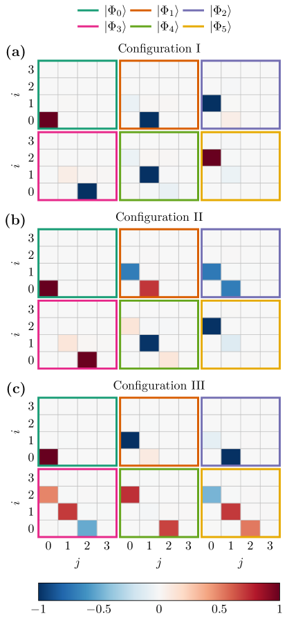
Figure 4: Two-body wave function coefficients $C_{ij,n}$ of the six lowest energy eigenstates for each configuration, as defined in Eq. (6). The indices on the $x$ and $y$-axes correspond to the Hartree product states involved with each coefficient, so that the coefficient at tile ($i$,$j$) is multiplied with the product state $\ket{\phi^{L}_{i}\phi^{R}_{j}}$ and summed into the expansion of each energy eigenstate. (a) Coefficients for configuration I. Each energy eigenstate is well approximated by a single Hartree product state. (b) Coefficients for configuration II. The first and second excited eigenstates are close to maximally entangled. (c) Coefficients for configuration III. Here, the third, fourth and fifth excited eigenstates are entangled.

The two-body coefficients $C_{ij,n}$ corresponding to the six lowest energy eigenstates, as defined in the ansatz (6), are depicted in Figure 4 for the three main configurations. These coefficients demonstrate a good convergence of our optimization algorithm towards the target wavefunctions presented in Eqs. (9) and (10). In configuration I, the two-body eigenstates are effectively described by single Hartree product states, indicating the suppression of electron-electron correlations when the potential wells are detuned. In contrast, the coefficients $C_{ij,n}$ for configurations II and III reveal a high degree of entanglement, which is quantified using von Neumann entropies. A closer inspection of these coefficients reveals the presence of small, undesired Hartree terms in the two-body wavefunctions. For instance, for the first excited state in configuration I, shown in Figure 4(a), we find

$$\ket{\Phi_{1}}_{\mathrm{I}}\approx\sqrt{0.995}\ket{01}+\sqrt{0.005}\ket{10}$$ (13)

with a corresponding entropy of $S_{1}\approx 0.04$. Furthermore, we find a small mixing in states $\ket{\Phi_{3}}$, $\ket{\Phi_{4}}$, and $\ket{\Phi_{5}}$, indicating residual correlations between the two electrons through interactions with higher energy states. The degree of these remaining correlations, quantified by the entropies $S_{n}$, show small but non-zero values for all excited energy states. The underlying factors contributing to these observations will be discussed within the framework of the effective Hamiltonian model presented in the following subsection.

For the first two excited states in configuration II, shown in Fig. 4(b), the many-body wavefunctions are approximately described by

$$\ket{\Phi_{1}}_{\mathrm{II}} \approx\sqrt{0.513}\ket{01}-\sqrt{0.487}\ket{10},$$ (14)

$$\ket{\Phi_{2}}_{\mathrm{II}} \approx\sqrt{0.487}\ket{01}+\sqrt{0.513}\ket{10},$$

which are almost identical to the maximally entangled states in Eq. (9). The entropy for these entangled states reach a maximum value of 1, as seen in Fig. 3(b). Here too, none of the higher excited states can be entirely described by single product states indicating to a presence of small residual correlations. The entropies of the eigenstates $\ket{\Phi_{3}}$, $\ket{\Phi_{4}}$ and $\ket{\Phi_{5}}$ for configuration II are around $0.11$, $0.23$ and $0.13$, respectively.

We display the coefficients of the energy eigenstates for configuration III in Figure 4(c). The three states involved in the triple avoided crossing are close to the target states given in Eq. (10):

$$\ket{\Phi_{3}}_{\mathrm{III}} \approx-\sqrt{0.259}\ket{02}+\sqrt{0.244}\ket{20}+\sqrt{0.497}\ket{11},$$

$$\ket{\Phi_{4}}_{\mathrm{III}} \approx\sqrt{0.461}\ket{02}+\sqrt{0.538}\ket{20}-\sqrt{0.001}\ket{11},$$

$$\ket{\Phi_{5}}_{\mathrm{III}} \approx\sqrt{0.279}\ket{02}-\sqrt{0.218}\ket{20}+\sqrt{0.502}\ket{11}.$$ (15)

In this configuration, however, an unwanted coupling is present in the first and second excited eigenstates $\ket{\Phi_{1}}$ and $\ket{\Phi_{2}}$. The degree of entanglement for these states is rather weak, as seen at $\lambda=1$ in Fig. 3(b); both eigenstates have an entropy of around $0.07$.

We note that Fig. 4 demonstrates that the Hartree states serve as approximate Schmidt states for all the energy eigenstates of our system, as mentioned in section II.4. This is clearly seen from this figure since each row and column have approximately one non-zero coefficient.

For the sake of visualization, we include in Appendices B and E the probability distributions of the one-body Hartree basis states (Fig. 6) and the particle densities of the two-body energy states (Fig. 7) for each of the three configurations.

III.2 Effective Hamiltonian

In addition to the numerical results above, we present a simplified model of the system to provide an intuitive understanding of the underlying coupling mechanism between the two electrons. For this purpose we expand both the electrostatic potential terms and the Coulomb interaction in our model Hamiltonian (Eq. (3)) around equilibrium positions $x_{L}$ and $x_{R}$ for the two electrons. These equilibrium positions are defined so that the first order terms in the displacements $\Delta{x}_{i}$ cancel each other, leaving only terms of second order and higher.

The Taylor expansion of the electrostatic potential around the equilibrium positions results in harmonic traps $\omega_{i}^{2}\Delta{x}_{i}^{2}/2$, with frequencies defined by the curvature of the electrostatic potential at the equilibrium positions. The Coulomb interaction between the two electrons can also be expanded in terms of the displacements $\Delta{x}_{i}$. Considering only up to second-order terms we obtain

$$\frac{\kappa}{|x_{1}-x_{2}|}\approx\frac{\kappa}{d}\Big{(}1-\frac{\Delta x_{1}-\Delta x_{2}}{d}+\frac{(\Delta x_{1}-\Delta x_{2})^{2}}{d^{2}}\Big{)},$$ (16)

where $d=x_{R}-x_{L}$ is the distance between the two electrons in equilibrium. The total potential energy of the system in displacement-dependent terms takes the form

$$U_{\mathrm{C}}\approx\sum_{i=\mathrm{1,2}}\frac{(\omega_{i}^{2}+\omega_{\mathrm{C}}^{2})}{2}\Delta x_{i}^{2}+\omega_{\mathrm{C}}^{2}\Delta x_{1}\Delta x_{2},$$ (17)

where $\omega_{\mathrm{C}}^{2}=2\kappa/d^{3}$. The first term in this equation describes how the Coulomb interaction effectively modifies the potential wells from the electrostatic potential. This is similar to the Hartree method since it computes an effective mean potential for each electron, created by the other electron in the system, however it is also different in that it treats the electrons as point particles instead of quantum particles. The last term in Eq. (17) gives rise to correlations between the two electrons. By introducing canonical transformations for the displacements and applying the rotating wave approximation, the Hamiltonian of the system takes the form

$$\hat{H}\approx\omega^{L}\hat{a}^{\dagger}\hat{a}+\omega^{R}\hat{b}^{\dagger}\hat{b}+g(\hat{a}^{\dagger}\hat{b}+\hat{a}\hat{b}^{\dagger}),$$ (18)

where $\hat{a}$ and $\hat{b}$ are ladder operators of displacement in the left and right wells respectively, $(\omega^{L})^{2}=\omega_{1}^{2}+\omega_{\mathrm{C}}^{2}$ and $(\omega^{R})^{2}=\omega_{2}^{2}+\omega_{\mathrm{C}}^{2}$ are modified vibrational frequencies and $g=\omega_{\mathrm{C}}^{2}/2\sqrt{\omega^{L}\omega^{R}}$ describes the interaction strength.

This Hamiltonian is diagonalized by a standard Bogoliubov transformation $U_{\theta}=\exp(\theta(\hat{a}^{\dagger}\hat{b}-\hat{a}\hat{b}^{\dagger}))$ with a rotation angle $2\theta=\arctan(2g/\Delta)$ [64]. The resulting Hamiltonian takes the diagonal form $\hat{H}=\Omega^{+}\hat{\alpha}^{\dagger}\hat{\alpha}+\Omega^{-}\hat{\beta}^{\dagger}\hat{\beta}$. Here $\hat{\alpha}$ and $\hat{\beta}$ are the transformed ladder operators, and the eigenfrequencies of the corresponding hybridized modes are given by

$$\Omega^{\pm}=\frac{1}{2}\Big{(}\omega^{L}+\omega^{R}\pm\sqrt{4g^{2}+\Delta^{2}}\Big{)}.$$ (19)

$\Delta=\omega^{L}-\omega^{R}$ is the detuning between the two wells as defined in Sec. II.6.

Given the multilevel nature of electronic states in each well, one has to carefully treat the unitary transformation of the effective Hamiltonian in Eq. (18). Including the anharmonicity of each oscillator as additional terms $\beta^{L}\hat{a}^{\dagger}\hat{a}(\hat{a}^{\dagger}\hat{a}-1)/2$ and $\beta^{R}\hat{b}^{\dagger}\hat{b}(\hat{b}^{\dagger}\hat{b}-1)/2$ in the Hamiltonian, which corresponds to including quartic terms in the expansion of the electrostatic potential, results in correlations emerging from interactions between the higher energy states. After performing a Bogoliubov transformation $U_{\theta}$ similar to the one above, the term corresponding to the anharmonicities takes the form

$$\hat{H}_{ZZ}=\frac{\zeta}{2}\hat{\alpha}^{\dagger}\hat{\alpha}\hat{\beta}^{\dagger}\hat{\beta},$$ (20)

where $\zeta$ is given by

$$\zeta=\sqrt{2}g\Big{(}\tan{\frac{\theta_{R}}{2}}-\tan{\frac{\theta_{L}}{2}}\Big{)},$$ (21)

with $\tan{\theta_{L\atop R}}=2\sqrt{2}g/(\Delta\pm\beta^{L\atop R})$ [84]. The quantity $\zeta$ corresponds to the energy shift defined in Eq. (11), and is the result of interactions between the $\ket{20}$ and $\ket{02}$ states and the $\ket{11}$ state.

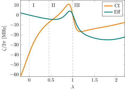
Figure 5: The energy difference $\zeta$ defined in Eq. (11). The orange line represents results from the numerical solution of the full two-body problem, whereas the teal line shows $\zeta$ values calculated from the effective Hamiltonian approach. Frequencies obtained from Hartree energies and a fixed coupling strength determined at the avoided crossing of configuration II were used in the effective model calculations. Configurations I, II and III are marked with vertical dashed lines at their respective $\lambda$ values of $0$, $0.46$ and $1$.

In general, unwanted correlations from this type of interactions lead to a conditional phase accumulation on the electron’s states as discussed in section II.5. In Fig. 5 we show calculations of $\zeta$ from our CI calculations and from the effective Hamiltonian approach. In the framework of the effective Hamiltonian this quantity strongly depends on the relative signs of the anharmonicities, which can be seen from the expression (21). For small $\theta_{L\atop R}\ll 1$ values, which are realized in configuration I, the coupling strength can be approximated by $\zeta\approx 2g^{2}/(\Delta+\beta^{L})-2g^{2}/(\Delta-\beta^{R})$. This vanishes at equal but opposite sign anharmonicities of two electrons. However, the CI calculations show a strong deviation of $\zeta$ from the predictions based on the effective model for well configurations $\lambda<0.5$ and $\lambda>1.5$ (see Fig. 5). We argue that these residual correlations appear due to a complexity in the shape of the potential wells. Nonlinearities on the localization length scale of electrons requires us to include of higher-order terms in the Taylor expansion of the electrostatic and Coulomb potentials. These terms, together with the anharmonicities, can change for different voltage configurations, a feature which further complicates our model. These intricacies are inherent to the electrostatic field generated by the array of electrodes in the micro-device considered. Potentially, the $ZZ$ coupling strength can be included in the configurational search as another minimization parameter to further suppress such correlations between the two electrons.

The effective Hamiltonian presented in Eq. (18), represents one of the most elementary models for describing coupled two-qubit systems. This model finds widespread use in various superconducting qubit architectures. Its simplicity in form facilitates the mapping of diverse entangling gates from these platforms to our system. However, alongside the simplicity of this model, we have illustrated its limitations when comparing its predictions with the results of full configuration interaction (CI) calculations. These limitations need to be handled thoughtfully in order to account for all potential sources of entanglement. Addressing these limitations becomes crucial for providing an accurate and complete description of the entanglement dynamics within the system and will be the scope of future work.

IV Conclusions

The results presented in this work highlight how the Coulomb interaction can induce motional entanglement between electronic states localized in separate wells above the surface of superfluid helium. To find the optimal specific device parameters for generating the entangled states, we have developed an optimization method based on many-body methods like full-configuration interaction (CI) theory [63] together with effective optimization algorithms. Our optimization methodology allows us to determine the optimal voltage configuration on the device electrodes needed to generate entanglement. In this way, the many-body-physics-based methodology we have developed has the potential to serve as a valuable tool to guide experimental work and inform future device design.

As an illustration, in this work we examined three distinct device parameter configurations (I, II, and III), leading to different types of entanglement between the two electrons. The tunability of the micro-device allows us to adjust the applied voltages and dynamically create highly anharmonic electrostatic traps, even with varying signs of anharmonicity. This tunability offers precise control over the potential landscape experienced by the electrons and allows for the tailoring of trapping potentials for specific experimental requirements, such as the experimental realization of specific gates and operations on the electronic qubits. Additionally we employed an effective Hamiltonian to approximate the two-electron system, which was in turn compared with our exact CI calculations, allowing us to investigate the limitations of the approximations used to construct this effective model. This comparison holds promise for a more detailed understanding of errors in the simulation of quantum devices based on this trapped electron system.

Finally, recent theoretical investigations have explored the dynamics and decoherence of electron spins above the surface of liquid helium [47]. These studies considered the role of spin-orbit interactions, which can be artificially enhanced by applying a spatially inhomogeneous magnetic field parallel to the helium surface. In future studies the methodology developed in our work can be extended to investigate entangling interactions between spins, devices containing spatially varying magnetic fields, as well as dynamical driving fields to investigate the time-dependence of entangled charge states and spin states.

In addition to studies of the time evolution of these quantum mechanical systems and thereby the temporal evolution of entangled states, we plan to extend our studies to more than two particles, with the aim to explore the experimental realization of many-body entanglement for electrons above the surface of liquid helium and solid neon. The hope is that these theoretical tools can guide studies of entanglement, development of experimental devices and realization of quantum gates and circuits for systems of many trapped and interacting electrons.

Appendix A Constructing the single-particle basis sets

For our numerical calculations we use a pseudo-spectral basis, i.e., a discrete variable representation (DVR), and adopt a linear interpolation for the coupling constants $\alpha_{i}(x)$. Specifically, we use the one-dimensional $\operatorname{sinc}$-DVR basis suggested by Colbert and Miller [88]. After dividing the Hamiltonian into two distinguishable subsystems $L$ and $R$, as shown in Eq. (5), we establish two $\operatorname{sinc}$-DVR basis sets, one for each well. We denote these basis functions by $B^{A}=\quantity{\chi^{A}_{\alpha}(x)\mid\alpha=0,\dots,K^{A}}$ with the corresponding quadrature of collocation points and weights $Q^{A}=\quantity{(x^{A}_{\alpha},w^{A}_{\alpha})\mid\alpha=0,\dots,K^{A}}$ for $A\in\quantity{L,R}$. The quadrature is uniform for the $\operatorname{sinc}$-DVR basis, meaning that $w^{A}_{\alpha}=\Delta x^{A}$ and $x^{A}_{\alpha+1}=x^{A}_{\alpha}+\Delta x^{A}$ for all $\alpha$.

We let $x^{L}_{K^{L}+1}=x_{b}=x^{R}_{0}$, i.e., the barrier is only included as a quadrature point in the right system, and we let $\Delta x=\Delta x^{L}=\Delta x^{R}$. The $\operatorname{sinc}$-DVR functions are then given by

$$\chi^{A}_{\alpha}(x)=\frac{1}{\sqrt{\Delta x}}\operatorname{sinc}\!\quantity(\frac{x-x^{A}_{\alpha}}{\Delta x}),$$

with

$$\operatorname{sinc}(x)=\begin{cases}\frac{\sin(\pi x)}{\pi x},&x\neq 0,\\ \hfil 1,&x=0.\end{cases}$$

This means that $\chi^{A}_{\alpha}(x^{A}_{\beta})=(\Delta x)^{-1/2}\delta_{\alpha\beta}$ on the quadrature. By restricting the grid on each side only up to the barrier, we have effectively established an infinite potential wall. This means that the potentials given in Eq. (4) are altered to

$$v^{L}(x)=\begin{cases}v(x),&x<x_{b},\\ \infty,&x\geq x_{b},\end{cases}$$

$$v^{R}(x)=\begin{cases}\infty,&x<x_{b},\\ v(x),&x\geq x_{b}.\end{cases}$$

This forces each electron to remain in its own well, and might seem an extreme limitation. However, the results in our model are completely unchanged, and it is much more computationally efficient and practical to use two separate basis sets.

The matrix elements of the kinetic energy operator are given by [88]

$$t^{A}_{\alpha\beta} =\matrixelement*{\chi^{A}_{\alpha}}{-\frac{1}{2}\derivative[2]{x}}{\chi^{A}_{\beta}}=\begin{cases}\frac{\pi^{2}}{6(\Delta x)^{2}},&\alpha=\beta,\\ \frac{(-1)^{\alpha-\beta}}{(\Delta x)^{2}(\alpha-\beta)^{2}},&\alpha\neq\beta,\end{cases}$$

and the external potential is approximated using the quadrature rule, viz.,

$$v^{A}_{\alpha\beta} =\matrixelement*{\chi^{A}_{\alpha}}{\hat{v}^{A}(x)}{\chi^{A}_{\beta}}$$

$$\approx\Delta x\sum_{\gamma=0}^{K^{A}}\chi^{A}_{\alpha}(x^{A}_{\gamma})v^{A}(x^{A}_{\gamma})\chi^{A}_{\beta}(x^{A}_{\gamma})=\delta_{\alpha\beta}v^{A}(x^{A}_{\beta}),$$

that is, the potential is diagonal. The matrix elements of the full one-body Hamiltonian can then be written

$$h^{A}_{\alpha\beta} =t^{A}_{\alpha\beta}+\delta_{\alpha\beta}v^{A}_{\beta},$$

where we have defined the diagonal potential matrix elements $v^{A}_{\beta}\equiv v^{A}(x^{A}_{\beta})$.

To evaluate the two-body Coulomb interaction, we examine the matrix elements of tensor products of DVR-states., i.e., $\ket*{\chi^{L}_{\alpha}\chi^{R}_{\beta}}=\ket*{\chi^{L}_{\alpha}}\otimes\ket*{\chi^{R}_{\beta}}$. We also use the convention that $\bra*{\chi^{L}_{\alpha}\chi^{R}_{\beta}}=\bra*{\chi^{L}_{\alpha}}\otimes\bra*{\chi^{R}_{\beta}}=\ket*{\chi^{L}_{\alpha}\chi^{R}_{\beta}}^{\dagger}$ for the conjugate states. We are able to directly compute the matrix elements of the soft Coulomb interaction operator using the quadrature rule. The matrix elements are thus

$$u_{\alpha\beta,\gamma\delta} =\matrixelement*{\chi^{L}_{\alpha}\chi^{R}_{\beta}}{\hat{u}(x_{1},x_{2})}{\chi^{L}_{\gamma}\chi^{R}_{\delta}}$$

$$\approx\Delta x^{L}\Delta x^{R}\sum_{\sigma=0}^{K^{L}}\sum_{\tau=0}^{K^{R}}\chi^{L}_{\alpha}(x^{L}_{\sigma})\chi^{R}_{\beta}(x^{R}_{\tau})u(x^{L}_{\sigma},x^{R}_{\tau})$$

$$\qquad\times\chi^{L}_{\gamma}(x^{L}_{\sigma})\chi^{R}_{\delta}(x^{R}_{\tau})$$

$$=\delta_{\alpha\gamma}\delta_{\beta\delta}u(x^{L}_{\gamma},x^{R}_{\delta}),$$

which is diagonal for each particle axis. We label the matrix elements of the diagonal Coulomb operator by $u^{LR}_{\gamma\delta}\equiv u(x^{L}_{\gamma},x^{R}_{\delta})$.

Appendix B The Hartree method

In the Hartree method for two distinguishable particles we approximate the ground state $\ket*{\Phi_{0}}$ of the full Hamiltonian $\hat{H}$ in Eq. (2) as the product state $\ket*{\Phi_{0}}\approx\ket*{\Psi}=\ket*{\phi^{L}_{0}\phi^{R}_{0}}$ under the constraint that the Hartree orbitals are orthonormal, i.e., $\innerproduct*{\phi^{A}_{0}}{\phi^{A}_{0}}=1$. This lets us set up the following Lagrangian

$$L=E_{H}-\lambda^{L}\quantity(\innerproduct*{\phi^{L}_{0}}{\phi^{L}_{0}}-1)-\lambda^{R}\quantity(\innerproduct*{\phi^{R}_{0}}{\phi^{R}_{0}}-1),$$

where $\lambda^{A}$ are Lagrange multipliers, and the Hartree energy $E_{H}=\matrixelement*{\Psi}{\hat{H}}{\Psi}$ is given by

$$E_{H}=\matrixelement*{\phi^{L}_{0}}{\hat{h}^{L}}{\phi^{L}_{0}}+\matrixelement*{\phi^{R}_{0}}{\hat{h}^{R}}{\phi^{R}_{0}}+\matrixelement*{\phi^{L}_{0}\phi^{R}_{0}}{u}{\phi^{L}_{0}\phi^{R}_{0}}.$$

Our next objective is to minimize the Lagrangian with respect to the Hartree states and the multipliers. To do this we expand the Hartree states as a linear combination of $\operatorname{sinc}$-DVR states:

$$\ket*{\phi^{A}_{i}}=\sum_{\alpha=0}^{K^{A}}B^{A}_{\alpha i}\ket*{\chi^{A}_{\alpha}},$$ (22)

and minimize with respect to the coefficients $B^{A}_{\alpha i}$. Computing $\partial L/\partial{B^{A}_{\alpha 0}}^{*}=0$ gives two coupled eigenvalue equations

$$\begin{gathered}\sum_{\beta=0}^{K^{L}}\underbrace{\quantity(h^{L}_{\alpha\beta}+\delta_{\alpha\beta}\sum_{\gamma=0}^{K^{R}}\absolutevalue{B^{R}_{\gamma 0}}^{2}u^{LR}_{\beta\gamma})}_{\equiv f^{L}_{\alpha\beta}}B^{L}_{\beta 0}=\lambda^{L}B^{L}_{\alpha 0},\\ \sum_{\beta=0}^{K^{R}}\underbrace{\quantity(h^{R}_{\alpha\beta}+\delta_{\alpha\beta}\sum_{\gamma=0}^{K^{L}}\absolutevalue{B^{L}_{\gamma 0}}^{2}u^{LR}_{\gamma\beta})}_{\equiv f^{R}_{\alpha\beta}}B^{R}_{\beta 0}=\lambda^{R}B^{R}_{\alpha 0},\end{gathered}$$ (23)

that needs to be solved iteratively until self-consistency has been achieved. The Hartree matrices $f^{A}_{\alpha\beta}$ are defined as everything inside the parentheses in the equations above. By diagonalizing the Hartree matrices, we obtain $K^{A}$ eigenvalues and eigenvectors, not just the lowest pair $\lambda^{A}$ and $B^{A}_{\alpha 0}$. We select the $N^{A}+1$ lowest eigenvectors, which gives us the set $P^{A}=\quantity{\ket{\phi^{A}_{i}}\mid i=0,\dots,N^{A}}$, where $N^{A}\ll K^{A}$.

The equations we solve are $\hat{f}^{A}\ket*{\phi^{A}_{i}}=\epsilon^{A}_{i}\ket*{\phi^{A}_{i}}$, where $\hat{f}^{A}$ is the Hartree matrix defined earlier, and $\epsilon^{A}_{i}$ are the eigenvalues with the corresponding eigenvectors $\ket*{\phi^{A}_{i}}$. These eigenvalues describe the energy felt by a single particle trapped in one of the wells under the influence of a charge in the other well. Formulated in terms of the coefficients, the equations are

$$\sum_{\beta=0}^{K^{A}}f^{A}_{\alpha\beta}B^{A}_{\beta i}=\epsilon^{A}_{i}B^{A}_{\alpha i},$$

with $f^{A}_{\alpha\beta}$ being the Hartree matrices from Eqs. (23). These equations are solved iteratively until a convergence of $\absolutevalue{\epsilon^{A,(k+1)}_{i}-\epsilon^{A,(k)}_{i}}<\delta\epsilon$ with $\delta\epsilon=$1\text{\times}{10}^{-10}$$ has been reached. Here $k$ corresponds to an iteration number. We choose $f^{A,(0)}_{\alpha\beta}=h^{A}_{\alpha\beta}$ as an initial state such that

$$\sum_{\beta=0}^{K^{A}}h^{A}_{\alpha\beta}B^{A,(0)}_{\beta i}=\epsilon^{A,(0)}_{i}B^{A,(0)}_{\alpha i}.$$

For the three target configurations found through numerical optimization in this work, the probability distributions of the first four Hartree states in each well are plotted in Fig. 6.

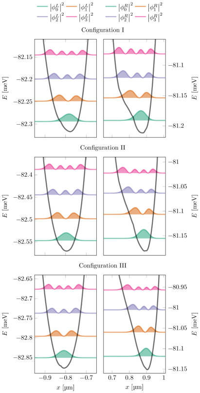
Figure 6: Probability distributions of the first four Hartree states in the left and right wells for all three configurations, shifted upwards with their Hartree transition frequencies from the respective ground states (in teal). The effective potentials for each subsystem, i.e., the well potential set up by the electrodes plus the mean-field contribution from the other electron, are plotted as dashed lines. As in Fig. 7 the left y-axis applies to the transition frequencies, while the right y-axis applies to the potentials, here for both panes.

Appendix C Full configuration-interaction for two distinguishable particles

Once the Hartree equations are solved, we obtain the coefficients $B^{A}_{\alpha i}$, which allow us to construct the Hartree basis $P^{A}$ from the $\operatorname{sinc}$-DVR basis $B^{A}$ using Eq. (22). We can perform a basis transformation from the $\operatorname{sinc}$-DVR basis to the smaller Hartree basis by using relations:

$$h^{A}_{ij}=\sum_{\alpha=0}^{K^{A}}\sum_{\beta=0}^{K^{A}}B^{A*}_{\alpha i}B^{A}_{\beta j}h^{A}_{\alpha\beta},$$ (24)

$$u_{ij,kl}=\sum_{\alpha=0}^{K^{L}}\sum_{\beta=0}^{K^{R}}B^{L*}_{\alpha i}B^{R*}_{\beta j}B^{L}_{\alpha k}B^{R}_{\beta l}u^{LR}_{\alpha\beta},$$ (25)

where greek letters denote matrix elements in the $\operatorname{sinc}$-DVR basis, and latin letters are for the Hartree basis.

Upon inserting the wave function ansatz into the time-independent Schrödinger equation and projecting onto a two-body state $\bra*{\phi^{L}_{i}\phi^{R}_{j}}$, we get:

$$\matrixelement*{\phi^{L}_{i}\phi^{R}_{j}}{\hat{H}}{\Phi_{n}} =\sum_{k=0}^{N^{L}}\sum_{l=0}^{N^{R}}H_{ij,kl}C_{kl,n}=C_{ij,n}E_{n},$$

where $H_{ij,kl}\equiv\matrixelement*{\phi^{L}_{i}\phi^{R}_{j}}{\hat{H}}{\phi^{L}_{k}\phi^{R}_{l}}$ are the matrix elements of the Hamiltonian in the Hartree product basis. The solution of this eigenvalue equation yields the coefficients $C_{ij,n}$, where each column corresponds to an eigenstate $\ket{\Phi_{n}}$ with corresponding eigenenergy $E_{n}$. The matrix elements of the two-body Hamiltonian can be expressed as:

$$H_{ij,kl} =h^{L}_{ik}\delta_{jl}+\delta_{ik}h^{R}_{jl}+u_{ij,kl},$$

where the one- and two-body matrix elements in the Hartree basis are shown in Eqs. (24) and (25).

Appendix D The von Neumann entropy

The von Neumann entropy is defined by

$$S=-\tr\!\quantity(\hat{\rho}\log_{2}(\hat{\rho})),$$

where $\hat{\rho}$ is the density operator. The entropy of the eigenstates $\ket*{\Phi_{n}}$ will be zero as they are pure states. However, the entropy of the reduced subsystems ($L$ and $R$) of $\ket*{\Phi_{n}}$ will in general not be zero. Each subsystem will have the same entropy, and any non-zero entropy can be attributed to entanglement. We can evaluate the entanglement entropy by bypassing the construction of the reduced density operator and using the Schmidt decomposition instead. Specifically, for a given two-body wave function $\ket*{\Psi}$ expressed in terms of the Hartree product states,

$$\ket*{\Psi}=\sum_{k=0}^{N^{L}}\sum_{l=0}^{N^{R}}C_{kl}\ket*{\phi^{L}_{k}\phi^{R}_{l}},$$

we can perform a singular value decomposition of the two-body coefficients, $C_{kl}=\sum_{p=0}^{\tilde{N}}U_{kp}\sigma_{p}V^{*}_{lp}$, to obtain

$$\ket*{\Psi}=\sum_{p=0}^{\tilde{N}}\sigma_{p}\ket*{\psi^{L}_{p}\psi^{R}_{p}},$$

where

$$\ket*{\psi^{L}_{p}}\equiv\sum_{k=0}^{N^{L}}U_{kp}\ket*{\phi^{L}_{k}},\qquad\ket*{\psi^{R}_{p}}\equiv\sum_{l=0}^{N^{R}}V^{*}_{lp}\ket*{\phi^{R}_{l}},$$

are the Schmidt states, $\tilde{N}$ is either $N^{L}$ or $N^{R}$ depending on the definition of the singular value decomposition, and $\sigma_{p}$ are the singular values with $\sigma_{p}^{2}$ representing the occupation of the single-particle states $\ket*{\psi^{L}_{p}}$ and $\ket*{\psi^{R}_{p}}$. Using the singular values, we can then compute the von Neumann entropy of $\ket{\Psi}$ as follows:

$$S=-\sum_{p=0}^{\tilde{N}}\sigma_{p}^{2}\log_{2}(\sigma_{p}^{2}).$$

Appendix E Particle densities

For the state $\ket{\Psi}$ above, we can compute the particle density by

$$\rho(x) =\int\differential{y}\absolutevalue{\Psi(x,y)}^{2}+\int\differential{y}\absolutevalue{\Psi(y,x)}^{2}$$

$$=\sum_{i,j=0}^{N^{L}}\sum_{l=0}^{N^{R}}C^{*}_{il}C_{jl}{\phi^{L}_{i}}^{*}(x)\phi^{L}_{j}(x)$$

$$\qquad+\sum_{i,j=0}^{N^{R}}\sum_{k=0}^{N^{L}}C^{*}_{ki}C_{kj}{\phi^{R}_{i}}^{*}(x)\phi^{R}_{j}(x),$$

which collapses to the electron density in the case of indistinguishable particles. The calculated particle densities for the three target configurations found through numerical optimization in this work are shown in Fig. 7.

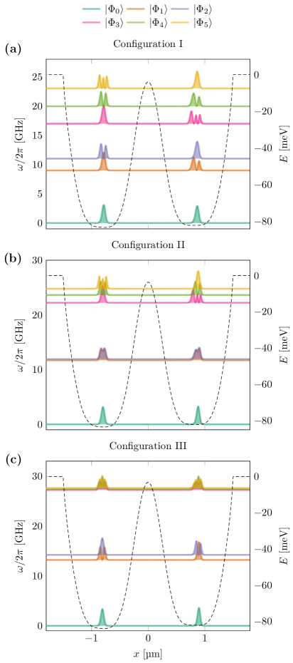
Figure 7: Calculated particle densities of the first six eigenstates of the full two-body Hamiltonian for configurations I (a), II (b) and III (c). Each state is shifted upwards with its transition frequency from the ground state (in teal). The electrostatic potential wells are shown by dashed lines. Note that these are hybrid plots; the left y-axis gives the unit scale for the transition frequencies, while the right y-axis gives the unit scale for the electrostatic potential energy.

Appendix F Finding optimal well configurations

In this appendix, we present a way of finding the optimal configuration for single motional qubit rotations, configuration I, as well as the optimal configurations for two-qubit operations, configuration II and III. These are found by expressing our configurational search in terms of an optimization problem. The seven voltages of the potential from Eq. (1), denoted $\bm{V}$, will be varied to find the optimal solution. We note that due to the flexibility provided by the potential, the optimization landscape consists of several local minima and the resulting voltages are therefore somewhat arbitrary. The same can also be said for the path between configurations. We have chosen configurations and a path such that our results resemble those of Fig. 2(b) by Zhao et al. [84], but we stress that our model allows for vastly different solutions. We select a fixed anharmonicity with equal magnitude and opposite sign for each well, and try to tune the wells such that only the detuning between each well is altered.

Configuration I is a configuration for which the transition frequencies are distinct, but at the same time within the working range of 5–$15\text{\,}\mathrm{GHz}$ of the read-out resonators. Furthermore, we aim for the anharmonicities in the left and right well, denoted as $\beta^{L}/2\pi$ and $\beta^{R}/2\pi$, to have equal magnitudes but with opposite signs. This adjustment is made to eliminate $ZZ$ crosstalk and facilitate a high on-off ratio for the implementation of controlled phase-gates. [85, 84]. There are several possible candidates for the transition frequencies and anharmonicities which satisfy these requirements, and the candidates we end up with are a result of performing the optimization process for a range of possible candidates. For the left well, we targeted a transition frequency between the two lowest energy levels of $\omega^{L}/2\pi=\epsilon^{L}_{1}-\epsilon^{L}_{0}=$11\text{\,}\mathrm{GHz}$$, and a corresponding transition frequency for the right well of $\omega^{R}/2\pi=\epsilon^{R}_{1}-\epsilon^{R}_{0}=$9\text{\,}\mathrm{GHz}$$. Here $\epsilon^{A}_{i}$ are the Hartree eigenvalues, i.e., the single-particle Hartree energies. At the same time, we targeted anharmonicites of $\beta^{L}/2\pi=-\beta^{R}/2\pi=$1\text{\,}\mathrm{GHz}$$. If we were allowed to vary the transition frequencies and anharmonicities independently and freely, a cost function with minima that coincide with these properties is

$$C_{\mathrm{I}}(\bm{V}) =(\omega^{L}(\bm{V})/2\pi-$11\text{\,}\mathrm{GHz}$)^{2}$$

$$+(\omega^{R}(\bm{V})/2\pi-$9\text{\,}\mathrm{GHz}$)^{2}$$

$$+(\beta^{L}(\bm{V})/2\pi-$1\text{\,}\mathrm{GHz}$)^{2}$$

$$+(\beta^{R}(\bm{V})/2\pi+$1\text{\,}\mathrm{GHz}$)^{2},$$ (26)

where $\omega^{A}(\bm{V})/2\pi$ is the transition frequency and $\beta^{A}(\bm{V})/2\pi$ is the anharmonicity of the wells (with $A\in\{L,R\}$). To minimize $C_{\mathrm{I}}(\bm{V})$ we evaluated its gradient with respect to the voltages, that is, $\nabla_{\bm{V}}C_{\mathrm{I}}(\bm{V})$, using the Tensorflow machine learning library [89]. We then used a variation of the gradient descent method with an adaptive learning rate based on the ADAM algorithm [87], to update the voltages. The learning rate for the Adam optimizer was initially set to $10^{-4}$.

For configuration III, we want to tune into a triple degeneracy point between the states $\ket{\Phi_{3}}$, $\ket{\Phi_{4}}$ and $\ket{\Phi_{5}}$. This allows for the realization of a controlled-phase gate [85, 86]. In such a configuration, we construct a cost function based on targeting the von Neumann entropies of the eigenstates $\ket{\Phi_{3}}$, $\ket{\Phi_{4}}$ and $\ket{\Phi_{5}}$ to be $S_{3}=1.5$, $S_{4}=1.0$ and $S_{5}=1.5$, respectively, while the entropies of the lower eigenstates should be kept minimal. We targeted the same anharmonicities as for configuration I, that is, $\beta^{L}/2\pi=-\beta^{R}/2\pi=$1\text{\,}\mathrm{GHz}$$. In order to end up with a configuration close to configuration I in parameter space, we utilized the parameters for configuration I, denoted $\bm{V}_{\mathrm{I}}$, as the initial guess in the optimization algorithm. Finally, we ensure that a linear sweep of voltages from configuration I to configuration III passes through configuration II by targeting a detuning $\Delta_{\mathrm{III}}/2\pi=(\omega^{L}-\omega^{R})/2\pi=$-1\text{\,}\mathrm{GHz}$$ for configuration III, as explained in section II.6. The cost function we will apply is given by

$$C_{\mathrm{III}}(\bm{V}) =S_{1}(\bm{V})^{2}$$

$$+S_{2}(\bm{V})^{2}$$

$$+(S_{3}(\bm{V})-1.5)^{2}$$

$$+(S_{4}(\bm{V})-1.0)^{2}$$

$$+(S_{5}(\bm{V})-1.5)^{2}$$

$$+(\beta^{L}(\bm{V})/2\pi-$1\text{\,}\mathrm{GHz}$)^{2}$$

$$+(\beta^{R}(\bm{V})/2\pi+$1\text{\,}\mathrm{GHz}$)^{2}$$

$$+(\omega^{L}(\bm{V})/2\pi-\omega^{R}(\bm{V})/2\pi+$1\text{\,}\mathrm{GHz}$)^{2}.$$ (27)

We used the same optimization method and learning rate as for configuration I.

Appendix G Optimized electrode voltages

The explicit values of the electrode voltages obtained for the three optimized configurations are shown in table 1 below.

Table 1: Electrode voltages for the three configurations I, II, and III, resulting in a total electrostatic potential given by Eq. (1).

	I [$\mathrm{mV}$]	II [$\mathrm{mV}$]	III [$\mathrm{mV}$]
$V_{1}$	297.45	296.41	295.17
$V_{2}$	152.33	155.01	158.23
$V_{3}$	344.36	342.63	340.56
$V_{4}$	-353.49	-354.66	-356.05
$V_{5}$	345.93	345.26	344.46
$V_{6}$	143.94	143.78	143.60
$V_{7}$	302.24	302.81	303.49

References

- Steffen et al. [2006] M. Steffen, M. Ansmann, R. C. Bialczak, N. Katz, E. Lucero, R. McDermott, M. Neeley, E. M. Weig, A. N. Cleland, and J. M. Martinis, Measurement of the entanglement of two superconducting qubits via state tomography, Science 313, 1423 (2006), https://science.sciencemag.org/content/313/5792/1423.full.pdf .
- Barends et al. [2014] R. Barends, J. Kelly, A. Megrant, A. Veitia, D. Sank, E. Jeffrey, T. C. White, J. Mutus, A. G. Fowler, B. Campbell, Y. Chen, Z. Chen, B. Chiaro, A. Dunsworth, C. Neill, P. O’Malley, P. Roushan, A. Vainsencher, J. Wenner, A. N. Korotkov, A. N. Cleland, and J. M. Martinis, Superconducting quantum circuits at the surface code threshold for fault tolerance, Nature 508, 500 (2014).
- Monroe et al. [1995] C. Monroe, D. M. Meekhof, B. E. King, W. M. Itano, and D. J. Wineland, Demonstration of a fundamental quantum logic gate, Phys. Rev. Lett. 75, 4714 (1995).
- Schmidt-Kaler et al. [2003] F. Schmidt-Kaler, H. Häffner, M. Riebe, S. Gulde, G. P. T. Lancaster, T. Deuschle, C. Becher, C. F. Roos, J. Eschner, and R. Blatt, Realization of the cirac–zoller controlled-not quantum gate, Nature 422, 408 (2003).
- Li et al. [2003] X. Li, Y. Wu, D. Steel, D. Gammon, T. H. Stievater, D. S. Katzer, D. Park, C. Piermarocchi, and L. J. Sham, An all-optical quantum gate in a semiconductor quantum dot, Science 301, 809 (2003), https://science.sciencemag.org/content/301/5634/809.full.pdf .
- Petta et al. [2005] J. R. Petta, A. C. Johnson, J. M. Taylor, E. A. Laird, A. Yacoby, H. D. Lukin, C. H. Marcus, H. P. Hanson, and A. C. Gossard, Coherent manipulation of coupled electron spins in semiconductor quantum dots, Science 309, 2180+ (2005).
- Lovett et al. [2003] B. W. Lovett, J. H. Reina, A. Nazir, and G. A. D. Briggs, Optical schemes for quantum computation in quantum dot molecules, Phys. Rev. B 68, 205319 (2003).
- Nazir et al. [2005] A. Nazir, B. W. Lovett, S. D. Barrett, J. H. Reina, and G. A. D. Briggs, Anticrossings in förster coupled quantum dots, Phys. Rev. B 71, 045334 (2005).
- Dutt et al. [2007] M. V. G. Dutt, L. Childress, L. Jiang, E. Togan, J. Maze, F. Jelezko, A. S. Zibrov, P. R. Hemmer, and M. D. Lukin, Quantum register based on individual electronic and nuclear spin qubits in diamond, Science 316, 1312 (2007), full publication date: Jun. 1, 2007.
- Neumann et al. [2010] P. Neumann, R. Kolesov, B. Naydenov, J. Beck, F. Rempp, M. Steiner, V. Jacques, G. Balasubramanian, M. L. Markham, D. J. Twitchen, S. Pezzagna, J. Meijer, J. Twamley, F. Jelezko, and J. Wrachtrup, Quantum register based on coupled electron spins in a room-temperature solid, Nature Physics 6, 249 (2010).
- Bernien et al. [2013] H. Bernien, B. Hensen, W. Pfaff, G. Koolstra, M. S. Blok, L. Robledo, T. H. Taminiau, M. Markham, D. J. Twitchen, L. Childress, and R. Hanson, Heralded entanglement between solid-state qubits separated by three metres, Nature 497, 86 (2013).
- Madjarov et al. [2020] I. S. Madjarov, J. P. Covey, A. L. Shaw, J. Choi, A. Kale, A. Cooper, H. Pichler, V. Schkolnik, J. R. Williams, and M. Endres, High-fidelity entanglement and detection of alkaline-earth rydberg atoms, Nature Physics 16, 857 (2020).
- Evered et al. [2023] S. J. Evered, D. Bluvstein, M. Kalinowski, S. Ebadi, T. Manovitz, H. Zhou, S. H. Li, A. A. Geim, T. T. Wang, N. Maskara, H. Levine, G. Semeghini, M. Greiner, V. Vuletic, and M. D. Lukin, High-fidelity parallel entangling gates on a neutral atom quantum computer (2023), arXiv:2304.05420 [quant-ph] .
- Feynman [1982] R. P. Feynman, Simulating physics with computers, International journal of theoretical physics 21, 467 (1982).
- Trabesinger [2012] A. Trabesinger, Quantum simulation, Nature Physics 8, 263 (2012).
- Georgescu et al. [2014] I. M. Georgescu, S. Ashhab, and F. Nori, Quantum simulation, Rev. Mod. Phys. 86, 153 (2014).
- Altman et al. [2021] E. Altman, K. R. Brown, G. Carleo, L. D. Carr, E. Demler, C. Chin, B. DeMarco, S. E. Economou, M. A. Eriksson, K.-M. C. Fu, M. Greiner, K. R. Hazzard, R. G. Hulet, A. J. Kollár, B. L. Lev, M. D. Lukin, R. Ma, X. Mi, S. Misra, C. Monroe, K. Murch, Z. Nazario, K.-K. Ni, A. C. Potter, P. Roushan, M. Saffman, M. Schleier-Smith, I. Siddiqi, R. Simmonds, M. Singh, I. Spielman, K. Temme, D. S. Weiss, J. Vučković, V. Vuletić, J. Ye, and M. Zwierlein, Quantum simulators: Architectures and opportunities, PRX Quantum 2, 017003 (2021).
- Carlson et al. [2018] J. Carlson, D. J. Dean, M. Hjorth-Jensen, D. Kaplan, J. Preskill, K. Roche, M. J. Savage, and M. Troyer, Quantum computing for theoretical nuclear physics, a white paper prepared for the u.s. department of energy, office of science, office of nuclear physics (2018).
- Klco and Savage [2020] N. Klco and M. J. Savage, Systematically localizable operators for quantum simulations of quantum field theories, Phys. Rev. A 102, 012619 (2020).
- Yamamoto and Doi [2022] A. Yamamoto and T. Doi, Toward nuclear physics from lattice qcd on quantum computers (2022), arXiv:2211.14550 [hep-lat] .
- Illa and Savage [2022] M. Illa and M. J. Savage, Basic elements for simulations of standard-model physics with quantum annealers: Multigrid and clock states, Phys. Rev. A 106, 052605 (2022).
- Bauer et al. [2022] C. W. Bauer, Z. Davoudi, A. B. Balantekin, T. Bhattacharya, M. Carena, W. A. de Jong, P. Draper, A. El-Khadra, N. Gemelke, M. Hanada, D. Kharzeev, H. Lamm, Y.-Y. Li, J. Liu, M. Lukin, Y. Meurice, C. Monroe, B. Nachman, G. Pagano, J. Preskill, E. Rinaldi, A. Roggero, D. I. Santiago, M. J. Savage, I. Siddiqi, G. Siopsis, D. V. Zanten, N. Wiebe, Y. Yamauchi, K. Yeter-Aydeniz, and S. Zorzetti, Quantum simulation for high energy physics (2022), arXiv:2204.03381 [quant-ph] .
- Smith et al. [2016] J. Smith, A. Lee, P. Richerme, B. Neyenhuis, P. W. Hess, P. Hauke, M. Heyl, D. A. Huse, and C. Monroe, Many-body localization in a quantum simulator with programmable random disorder, Nature Physics 12, 907 (2016).
- Hofstetter and Qin [2018] W. Hofstetter and T. Qin, Quantum simulation of strongly correlated condensed matter systems, Journal of Physics B: Atomic, Molecular and Optical Physics 51, 082001 (2018).
- Smith et al. [2019] A. Smith, M. S. Kim, F. Pollmann, and J. Knolle, Simulating quantum many-body dynamics on a current digital quantum computer, npj Quantum Information 5, 106 (2019).
- Peruzzo et al. [2014] A. Peruzzo, J. McClean, P. Shadbolt, M.-H. Yung, X.-Q. Zhou, P. J. Love, A. Aspuru-Guzik, and J. L. O’Brien, A variational eigenvalue solver on a photonic quantum processor, Nature Communications 5, 4213 (2014).
- Reiher et al. [2016] M. Reiher, N. Wiebe, K. Svore, D. Wecker, and M. Troyer, Elucidating reaction mechanisms on quantum computers, Proceedings of the National Academy of Sciences 114 (2016).
- Kandala et al. [2017] A. Kandala, A. Mezzacapo, K. Temme, M. Takita, M. Brink, J. M. Chow, and J. M. Gambetta, Hardware-efficient variational quantum eigensolver for small molecules and quantum magnets, Nature 549, 242 (2017).
- Greiner et al. [2002] M. Greiner, O. Mandel, T. Esslinger, T. W. Hänsch, and I. Bloch, Quantum phase transition from a superfluid to a mott insulator in a gas of ultracold atoms, Nature 415, 39 (2002).
- Hart et al. [2015] R. A. Hart, P. M. Duarte, T.-L. Yang, X. Liu, T. Paiva, E. Khatami, R. T. Scalettar, N. Trivedi, D. A. Huse, and R. G. Hulet, Observation of antiferromagnetic correlations in the hubbard model with ultracold atoms, Nature 519, 211 (2015).
- Ebadi et al. [2021] S. Ebadi, T. T. Wang, H. Levine, A. Keesling, G. Semeghini, A. Omran, D. Bluvstein, R. Samajdar, H. Pichler, W. W. Ho, S. Choi, S. Sachdev, M. Greiner, V. Vuletić, and M. D. Lukin, Quantum phases of matter on a 256-atom programmable quantum simulator, Nature 595, 227 (2021).
- Lanyon et al. [2011] B. Lanyon, C. Hempel, D. Nigg, M. Müller, R. Gerritsma, F. Zähringer, P. Schindler, J. Barreiro, M. Rambach, G. Kirchmair, M. Hennrich, P. Zoller, R. Blatt, and C. Roos, Universal digital quantum simulation with trapped ions, Science (New York, N.Y.) 334, 57 (2011).
- Monroe et al. [2021] C. Monroe, W. C. Campbell, L.-M. Duan, Z.-X. Gong, A. V. Gorshkov, P. W. Hess, R. Islam, K. Kim, N. M. Linke, G. Pagano, P. Richerme, C. Senko, and N. Y. Yao, Programmable quantum simulations of spin systems with trapped ions, Rev. Mod. Phys. 93, 025001 (2021).
- Aspuru-Guzik and Walther [2012] A. Aspuru-Guzik and P. Walther, Photonic quantum simulators, Nature Physics 8, 285 (2012).
- Alsing et al. [2023] P. Alsing, P. Battle, J. C. Bienfang, T. Borders, T. Brower-Thomas, L. D. Carr, F. Chong, S. Dadras, B. DeMarco, I. Deutsch, E. Figueroa, D. Freedman, H. Everitt, D. Gauthier, E. Johnston-Halperin, J. Kim, M. Kira, P. Kumar, P. Kwiat, J. Lekki, A. Loiacono, M. Loncar, J. R. Lowell, M. Lukin, C. Merzbacher, A. Miller, C. Monroe, J. Pollanen, D. Pappas, M. Raymer, R. Reano, B. Rodenburg, M. Savage, T. Searles, and J. Ye, Accelerating progress towards practical quantum advantage: The quantum technology demonstration project roadmap (2023), arXiv:2210.14757 [quant-ph] .
- Matthiesen et al. [2021] C. Matthiesen, Q. Yu, J. Guo, A. M. Alonso, and H. Häffner, Trapping electrons in a room-temperature microwave paul trap, Phys. Rev. X 11, 011019 (2021).
- Yu et al. [2022] Q. Yu, A. M. Alonso, J. Caminiti, K. M. Beck, R. T. Sutherland, D. Leibfried, K. J. Rodriguez, M. Dhital, B. Hemmerling, and H. Häffner, Feasibility study of quantum computing using trapped electrons, Phys. Rev. A 105, 022420 (2022).
- Platzman and Dykman [1999] P. M. Platzman and M. I. Dykman, Quantum computing with electrons floating on liquid helium, Science 284, 1967 (1999).
- Shirahama et al. [1995] K. Shirahama, S. Ito, H. Suto, and K. Kono, Surface study of liquid3he using surface state electrons, Journal of Low Temperature Physics 101, 439 (1995).
- Dykman et al. [2003] M. Dykman, P. Platzman, and P. Seddighrad, Qubits with electrons on liquid helium, Physical Review B 67, 155402 (2003).
- Dahm et al. [2003] A. J. Dahm, J. Heilman, I. Karakurt, and T. Peshek, Quantum computing with electrons on helium, Physica E: Low-dimensional Systems and Nanostructures 18, 169 (2003), 23rd International Conference on Low Temperature Physics (LT23).
- Schuster et al. [2010] D. I. Schuster, A. Fragner, M. I. Dykman, S. A. Lyon, and R. J. Schoelkopf, Proposal for manipulating and detecting spin and orbital states of trapped electrons on helium using cavity quantum electrodynamics, Phys. Rev. Lett. 105, 040503 (2010).
- Shi et al. [2014] X. Shi, L. Wei, and C. H. Oh, Quantum computation with surface-state electrons by rapid population passages, Science China Physics, Mechanics & Astronomy 57, 1718 (2014).
- Kawakami et al. [2023] E. Kawakami, J. Chen, M. Benito, and D. Konstantinov, Hybrid rydberg-spin qubit of electrons on helium (2023), arXiv:2303.03688 [cond-mat.mes-hall] .
- Lyon [2006a] S. A. Lyon, Spin-based quantum computing using electrons on liquid helium, Phys. Rev. A 74, 052338 (2006a).
- Dykman et al. [2023a] M. I. Dykman, O. Asban, Q. Chen, D. Jin, and S. A. Lyon, Spin dynamics in quantum dots on liquid helium, Phys. Rev. B 107, 035437 (2023a).
- Dykman et al. [2023b] M. Dykman, O. Asban, Q. Chen, D. Jin, and S. Lyon, Spin dynamics in quantum dots on liquid helium, Physical Review B 107, 035437 (2023b).
- Marty [1986a] D. Marty, Stability of two-dimensional electrons on a fractionated helium surface, Journal of Physics C: Solid State Physics 19, 6097 (1986a).
- Ikegami et al. [2009] H. Ikegami, H. Akimoto, and K. Kono, Nonlinear transport of the wigner solid on superfluid in a channel geometry, Phys. Rev. Lett. 102, 046807 (2009).
- Zhang et al. [2009] M. Zhang, H. Y. Jia, and L. F. Wei, Jaynes-cummings models with trapped electrons on liquid helium, Phys. Rev. A 80, 055801 (2009).
- Rees et al. [2016a] D. G. Rees, N. R. Beysengulov, Y. Teranishi, C.-S. Tsao, S.-S. Yeh, S.-P. Chiu, Y.-H. Lin, D. A. Tayurskii, J.-J. Lin, and K. Kono, Structural order and melting of a quasi-one-dimensional electron system, Phys. Rev. B 94, 045139 (2016a).
- Zou and Konstantinov [2022] S. Zou and D. Konstantinov, Image-charge detection of the rydberg transition of electrons on superfluid helium confined in a microchannel structure, New Journal of Physics 24, 103026 (2022).
- Papageorgiou et al. [2004] G. Papageorgiou, P. Glasson, K. Harrabi, V. Antonov, E. Collin, P. Fozooni, P. Frayne, M. Lea, Y. Mukharsky, and D. Rees, Counting individual trapped electrons on liquid helium, Applied Physics Letters 86 (2004).
- Rees et al. [2011a] D. G. Rees, I. Kuroda, C. A. Marrache-Kikuchi, M. Höfer, P. Leiderer, and K. Kono, Point-contact transport properties of strongly correlated electrons on liquid helium, Phys. Rev. Lett. 106, 026803 (2011a).
- Rees et al. [2012] D. G. Rees, H. Totsuji, and K. Kono, Commensurability-dependent transport of a wigner crystal in a nanoconstriction, Phys. Rev. Lett. 108, 176801 (2012).
- Yang et al. [2016] G. Yang, A. Fragner, G. Koolstra, L. Ocola, D. A. Czaplewski, R. J. Schoelkopf, and D. I. Schuster, Coupling an ensemble of electrons on superfluid helium to a superconducting circuit, Phys. Rev. X 6, 011031 (2016).
- Koolstra et al. [2019] G. Koolstra, G. Yang, and D. I. Schuster, Coupling a single electron on superfluid helium to a superconducting resonator, Nature communications 10, 1 (2019).
- Byeon et al. [2021] H. Byeon, K. Nasyedkin, J. R. Lane, N. R. Beysengulov, L. Zhang, R. Loloee, and J. Pollanen, Piezoacoustics for precision control of electrons floating on helium, Nature Communications 12, 4150 (2021).
- Rousseau et al. [2007] E. Rousseau, Y. Mukharsky, D. Ponarine, O. Avenel, and E. Varoquaux, Trapping electrons in electrostatic traps over the surface of 4he, Journal of Low Temperature Physics 148, 193 (2007).
- Bradbury et al. [2011a] F. R. Bradbury, M. Takita, T. M. Gurrieri, K. J. Wilkel, K. Eng, M. S. Carroll, and S. A. Lyon, Efficient clocked electron transfer on superfluid helium, Phys. Rev. Lett. 107, 266803 (2011a).
- Zhou et al. [2022a] X. Zhou, G. Koolstra, X. Zhang, G. Yang, X. Han, B. Dizdar, X. Li, R. Divan, W. Guo, K. W. Murch, D. I. Schuster, and D. Jin, Single electrons on solid neon as a solid-state qubit platform, Nature 605, 46 (2022a).
- Zhou et al. [2023] X. Zhou, X. Li, Q. Chen, G. Koolstra, G. Yang, B. Dizdar, Y. Huang, C. S. Wang, X. Han, X. Zhang, D. I. Schuster, and D. Jin, Electron charge qubit with 0.1 millisecond coherence time, Nature Physics 10.1038/s41567-023-02247-5 (2023).
- Cramer [2004] C. J. Cramer, Essentials of Computational Chemistry (Wiley, New York, 2004).
- Blais et al. [2021] A. Blais, A. L. Grimsmo, S. M. Girvin, and A. Wallraff, Circuit quantum electrodynamics, Rev. Mod. Phys. 93, 025005 (2021).
- Cole and Cohen [1969] M. W. Cole and M. H. Cohen, Image-Potential-Induced Surface Bands in Insulators, Physical Review Letters 23, 1238 (1969).
- Shikin [1971] V. Shikin, Some properties of surface electrons in liquid helium, Soviet Physics JETP 33, 387 (1971).
- Grimes et al. [1976] C. C. Grimes, T. R. Brown, M. L. Burns, and C. L. Zipfel, Spectroscopy of electrons in image-potential-induced surface states outside liquid helium, Phys. Rev. B 13, 140 (1976).
- Collin et al. [2002] E. Collin, W. Bailey, P. Fozooni, P. G. Frayne, P. Glasson, K. Harrabi, M. J. Lea, and G. Papageorgiou, Microwave saturation of the rydberg states of electrons on helium, Phys. Rev. Lett. 89, 245301 (2002).
- Wagner [1973] F. Wagner, Scattering of light by thermal ripplons on superfluid helium, J. Low. Temp. Phys. 13, 317 (1973).
- Lyon [2006b] S. Lyon, Spin-based quantum computing using electrons on liquid helium, Physical Review A 74, 052338 (2006b).
- Rees et al. [2011b] D. G. Rees, I. Kuroda, C. A. Marrache-Kikuchi, M. Höfer, P. Leiderer, and K. Kono, Point-contact transport properties of strongly correlated electrons on liquid helium., Physical review letters 106, 026803 (2011b).
- Rees et al. [2016b] D. G. Rees, N. R. Beysengulov, Y. Teranishi, C.-S. Tsao, S.-S. Yeh, S.-P. Chiu, Y.-H. Lin, D. A. Tayurskii, J.-J. Lin, and K. Kono, Structural order and melting of a quasi-one-dimensional electron system, Physical Review B 94, 045139 (2016b).
- Papageorgiou et al. [2005] G. Papageorgiou, P. Glasson, K. Harrabi, V. Antonov, E. Collin, P. Fozooni, P. G. Frayne, M. J. Lea, D. G. Rees, and Y. Mukharsky, Counting Individual Trapped Electrons on Liquid Helium, Applied Physics Letters 86, 153106 (2005), cond-mat/0405084 .
- Zhou et al. [2022b] X. Zhou, G. Koolstra, X. Zhang, G. Yang, X. Han, B. Dizdar, X. Li, R. Divan, W. Guo, K. W. Murch, D. I. Schuster, and D. Jin, Single electrons on solid neon as a solid-state qubit platform, Nature 605, 46 (2022b), 2106.10326 .
- Grimes and Adams [1979] C. C. Grimes and G. Adams, Evidence for a Liquid-to-Crystal Phase Transition in a Classical, Two-Dimensional Sheet of Electrons, Physical Review Letters 42, 795 (1979).
- Cirac and Zoller [1995] J. I. Cirac and P. Zoller, Quantum computations with cold trapped ions, Phys. Rev. Lett. 74, 4091 (1995).
- Marty [1986b] D. Marty, Stability of two-dimensional electrons on a fractionated helium surface, Journal of Physics C: Solid State Physics 19, 6097 (1986b).
- Bradbury et al. [2011b] F. Bradbury, M. Takita, T. Gurrieri, K. Wilkel, K. Eng, M. Carroll, and S. Lyon, Efficient clocked electron transfer on superfluid helium, Physical Review Letters 107, 266803 (2011b).
- Sheldon et al. [2016] S. Sheldon, E. Magesan, J. M. Chow, and J. M. Gambetta, Procedure for systematically tuning up cross-talk in the cross-resonance gate, Physical Review A 93, 060302 (2016).
- Kvaal et al. [2007] S. Kvaal, M. Hjorth-Jensen, and H. M. Nilsen, Effective interactions, large-scale diagonalization, and one-dimensional quantum dots, Phys. Rev. B 76, 085421 (2007).
- Strauch et al. [2003] F. W. Strauch, P. R. Johnson, A. J. Dragt, C. J. Lobb, J. R. Anderson, and F. C. Wellstood, Quantum logic gates for coupled superconducting phase qubits, Phys. Rev. Lett. 91, 167005 (2003).
- DiCarlo et al. [2009] L. DiCarlo, J. M. Chow, J. M. Gambetta, L. S. Bishop, B. R. Johnson, D. Schuster, J. Majer, A. Blais, L. Frunzio, S. Girvin, et al., Demonstration of two-qubit algorithms with a superconducting quantum processor, Nature 460, 240 (2009).
- Nielsen and Chuang [2010] M. A. Nielsen and I. L. Chuang, Quantum Computation and Quantum Information (Cambridge University Press, 2010).
- Zhao et al. [2020] P. Zhao, P. Xu, D. Lan, J. Chu, X. Tan, H. Yu, and Y. Yu, High-contrast zz interaction using superconducting qubits with opposite-sign anharmonicity, Phys. Rev. Lett. 125, 200503 (2020).
- Ku et al. [2020] J. Ku, X. Xu, M. Brink, D. C. McKay, J. B. Hertzberg, M. H. Ansari, and B. L. T. Plourde, Suppression of unwanted zz interactions in a hybrid two-qubit system, Phys. Rev. Lett. 125, 200504 (2020).
- Xie et al. [2022] L. Xie, J. Zhai, Z. Zhang, J. Allcock, S. Zhang, and Y.-C. Zheng, Suppressing zz crosstalk of quantum computers through pulse and scheduling co-optimization, in Proceedings of the 27th ACM International Conference on Architectural Support for Programming Languages and Operating Systems, ASPLOS ’22 (Association for Computing Machinery, New York, NY, USA, 2022) p. 499–513.
- Kingma and Ba [2014] D. P. Kingma and J. Ba, Adam: A method for stochastic optimization (2014).
- Colbert and Miller [1992] D. T. Colbert and W. H. Miller, A novel discrete variable representation for quantum mechanical reactive scattering via the s‐matrix kohn method, The Journal of Chemical Physics 96, 1982 (1992).
- Abadi et al. [2015] M. Abadi, A. Agarwal, P. Barham, E. Brevdo, Z. Chen, C. Citro, G. S. Corrado, A. Davis, J. Dean, M. Devin, S. Ghemawat, I. Goodfellow, A. Harp, G. Irving, M. Isard, Y. Jia, R. Jozefowicz, L. Kaiser, M. Kudlur, J. Levenberg, D. Mané, R. Monga, S. Moore, D. Murray, C. Olah, M. Schuster, J. Shlens, B. Steiner, I. Sutskever, K. Talwar, P. Tucker, V. Vanhoucke, V. Vasudevan, F. Viégas, O. Vinyals, P. Warden, M. Wattenberg, M. Wicke, Y. Yu, and X. Zheng, TensorFlow: Large-scale machine learning on heterogeneous systems (2015), software available from tensorflow.org.