WAIT: Feature Warping for Animation to Illustration video Translation using GANs

Abstract

In this paper, we explore a new domain for video-to-video translation. Motivated by the availability of animation movies that are adopted from illustrated books for children, we aim to stylize these videos with the style of the original illustrations. Current state-of-the-art video-to-video translation models rely on having a video sequence or a single style image to stylize an input video. We introduce a new problem for video stylizing where an unordered set of images are used. This is a challenging task for two reasons: i) we do not have the advantage of temporal consistency as in video sequences; ii) it is more difficult to obtain consistent styles for video frames from a set of unordered images compared to using a single image.

Most of the video-to-video translation methods are built on an image-to-image translation model, and integrate additional networks such as optical flow, or temporal predictors to capture temporal relations. These additional networks make the model training and inference complicated and slow down the process. To ensure temporal coherency in video-to-video style transfer, we propose a new generator network with feature warping layers which overcomes the limitations of the previous methods. We show the effectiveness of our method on three datasets both qualitatively and quantitatively. Code and pretrained models are available at https://github.com/giddyyupp/wait.

I Introduction

Video-to-video translation aims to convert a given video in the source domain to a stylized version in the target domain. A successful translation should satisfy two important criteria; capturing target style, and ensuring temporal consistency between frames.

A natural solution for video-to-video translation is to extend the image-to-image translation methods by applying them on independent video frames. Although there are many successful image-to-image translation methods in the literature  [1, 2, 3, 4, 5, 6, 7, 8, 9], they only accomplish the first criteria. They are able to capture the target style, but they fail to ensure the temporal information in the video and create inconsistency between generated frames. Besides making each frame realistic, a video-to-video translation model should be capable of enhancing the temporal coherence between adjacent frames. Hence, domain specific methods [10, 11, 12, 13, 14, 15, 16] have emerged to address the shortcoming of image based models to achieve both aspects successfully.

The main approach to solve the inconsistency problem is to utilize additional information to capture temporal relations between frames. Optical flow is widely used in several methods to warp a stylized frame to estimate the next stylized frame or it is fed to a network to generate flow on the target domain and compare it with the source domain [10, 17, 18, 19, 20, 21]. However, there are two main problems in using optical flow; flow estimation is slow [15, 22]; and there are no real world data sets available with ground truth flow labels. Synthetic datasets introduce noise during training due to the domain gap [23, 24], and thus cannot be utilized efficiently.

Alternatively, specially designed temporal predictor networks [11], knowledge distillation [15], or feature transformations [25] are proposed to overcome inconsistency problem. Although these methods achieve on-par results, there are some flaws in their design which hinders their performance. For instance, ReCycleGan [11] feeds input frames independently diminishing the performance of the model, and optical flow is still used to train the teacher model in flow distillation [15].

Feature warping is an alternative approach to optical flow warping due to its efficiency and performance. Researchers utilize feature warping for pose estimation, object detection, classification, segmentation and tracking in videos [26, 27, 28, 29].

Inspired by the use of feature warping in detection tasks, our work pursuits the video counterpart by tackling unpaired video-to-video translation in a complex spatio-temporal context. Unlike previous methods that utilize optical flow or additional networks to ensure temporal consistency, our method integrates a feature warping network directly to the generator network. This simplifies the complicated architectures for video style transfer, in addition to faster train and test times. Also, its performance is on-par or better than the state-of-the-art methods.

Recently, some of the children books are adopted as animated movies. “Peter Rabbit" of Beatrix Potter and “ZOG" of Axel Scheffler are two of the examples. Although the characters are the same, the styles of the illustrations in books are different from animations. Motivated by these movies, we explore the problem of converting animation movies of children book characters into stylized versions of their original book illustrations for a specific illustrator.

However, in this setting, unlike the video-to-video translation problem, we do not have a target video, but only a set of unordered images in the style of the illustrator extracted from pages of the books. In this study, we attack this challenge and explore the use of unordered set of images on the target domain alternative to single image or a sequence of images from a target video. This setting eliminates the main challenges for these two approaches; need for collecting sequential data which is not always available and costly and trying to extract style information using just a single image which hardens the video stylization problem.

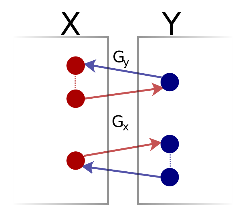
(a) CycleGAN [1]

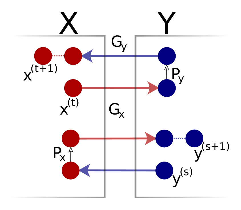
(b) ReCycleGAN [11]

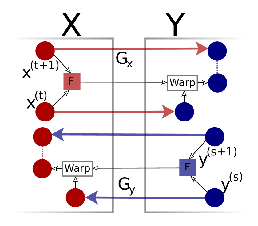
(c) OpticalFlowWarp [30]

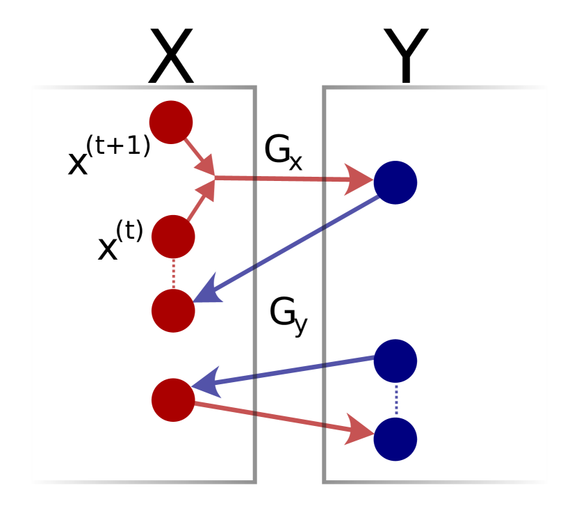
(d) WAIT

Figure 1: High level comparisons of baseline models and the proposed method WAIT. (a) CycleGAN contains two generator networks. These networks successfully capture the target styles but fails to ensure temporal coherency. (b) ReCycleGAN, contains two additional temporal predictor networks $P_{X}$ and $P_{Y}$ on top of CycleGAN to fulfill the missing feature, temporal relations. $P_{X}$ and $P_{Y}$ takes two previous frames, $X_{t}$ and $X_{t-1}$, and predicts the next frame $X_{t+1}$. (c) OpticalFlowWarping uses Optical Flow to capture temporal relations between generated frames. Rectangle boxes correspond to an pretrained optical flow prediction network. Predicted flow values are used to warp with a previously generated frame to get stylized current frame. (d) Our method WAIT contains just two networks $G_{X}$ and $G_{Y}$ to both capture target style and temporal coherency. Our model does not have any external network components and it is design is as simple as CycleGAN. Instead our method incorporates temporal information through feature warping layers inside the generator network. For all the models, dashed lines display the loss calculations specific to the model.

In summary, our study provides two major contributions to video style transfer problem: a new task to convert source videos of animation movies into the styles of arbitrarily selected pages from illustrations in the target domain; and a new method based on a generator network with feature warping layers, which is shown to be effective not only on task specific datasets but also on general purpose datasets. We refer to our method as “feature Warping for Animation to Illustration video Translation” or WAIT in short.

In the following, after reviewing the related literature II, we first describe both image-to-image and video-to-video translation methods that are served as baselines, then we present our method WAIT in detail III. Section IV explains the datasets used in the experiments. Finally, in Section V, we demonstrate effectiveness of our method using qualitative and quantitative analysis on three challenging dataset, and we validate the design chose of WAIT using detailed ablation experiments.

II Related Work

In this section, we first explain prominent GAN based image-to-image translation methods as the basis. Then, we elaborate on video-to-video translation methods.

Image-to-Image Translation: Recently, several methods have been proposed for image-to-image translation [2, 4, 1, 5, 3, 31, 32, 33, 9, 8]. CycleGAN [1] and DualGAN [5] are the pioneering unpaired image-to-image translation approaches. Both utilize a cyclic framework which consists of a couple of generators and discriminators. First couple learns a mapping from the source to the target, while the second one learns a reverse mapping. MUNIT [8] further improves unpaired image translation to multi-modal settings. First, source and target images are encoded into separate content and style latent spaces, and then they are decoded back to image domain by merging latent vectors.

Video-to-Video Translation: Even though, aforementioned image-to-image translation methods generate visually appealing images for each frame, they fail to capture temporal coherency and suffers from flickering artifacts [34]. To overcome this artifacts and to ensure temporal consistency between generated frames, video-to-video translation methods utilize temporal modules [17, 10, 30, 12, 21, 19, 34].

The dominant approach for temporal consistency is to use optical flow. Several models utilize optical flow models to estimate flow between input or generated frames (or both). Then, this flow is used to warp frames and to ensure temporal consistency between warped and stylized images [34, 19, 10, 21, 17, 14, 30, 18, 35, 14, 36, 12, 37, 38, 39, 20, 40, 22, 41, 42].

In its most basic form [19], optical flow is estimated on the consecutive input frames. Then, this flow is warped with a previously stylized frame. Temporal loss is calculated between current stylized frame and warped stylized frame. In [12], optical flow is estimated using FlowNet [43] on both input frames and generated frames. Estimated flows for both sides are first translated to other domain using motion translators. These translated flows are used for warping and calculating the loss similar to [19]. This model requires 8 generators, 4 discriminators, 4 optical flow and 2 motion translation models forwards for just a single iteration.

In another line of studies, temporal predictor networks [11, 44, 13], knowledge distillation [15], 3D convolution models [45], feature transformations [25] and self supervision [16] are proposed to incorporate temporal relations. ReCycleGAN [11] is an extension of CycleGAN [1] with additional temporal predictors which aims to predict the next frame given two previous frames. This predicted frame is also translated to target domain and an additional loss is calculated between predicted and real frame.

In addition to natural grouping of the methods based on the supervision they have (i.e. supervised/paired or unsupervised/unpaired), current video-to-video translation methods could also be grouped into two categories based on the type of the target dataset (note that the source dataset is video sequences). The first category assumes that the target dataset contains a single style image. These methods [10, 34, 19] usually utilize feed forward Convolutional Neural Networks (CNN) to perform translation. They extend image based Neural Style Transfer (NST) for videos with the addition of temporal components. On the other hand, the second group considers the target domain to contain ordered sequence of frames. In [14, 11] Generative Adversarial Networks (GANs) are utilized. Similar to previous category, image-to-image translation baselines are usually extended with temporal networks and loss functions.

III Methods

Our goal is to learn a mapping $G_{X}:X\rightarrow Y$ where the source domain $X$ contains ordered sequence of frames taken from a cartoon animation movie, and the target domain $Y$ contains unordered set of images taken from illustration books. This task differs from current video-to-video translation tasks where target domain $Y$ contains either ordered sequences [11] or a single image [19, 13]. Since there is no ground truth available for the frames in the source domain, the problem falls into unpaired translation category. Before going into the details of the proposed model, first we will explain the baseline methods used. A high-level architectural description of the proposed WAIT model and comparison with baseline architectures are presented in Figure 1.

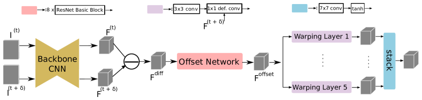
Figure 2: Detailed description of the generator network of WAIT. Our model takes two images, input frame $I_{t}$ and auxiliary frame $I_{t+\delta}$ as inputs and forwards them through the Backbone CNN to extract feature maps $F_{t}$ and $F_{t+\delta}$, respectively. Then, we calculate the difference of these two feature maps, $F_{diff}$. We forward this difference map to Offset Network and calculate offset features $F_{offset}$. As a final stage, we warp the offset features $F_{offset}$ with the auxiliary features $F_{t+\delta}$ to create final translated frame. Warping stage contains 5 parallel layers to capture features with different resolutions.

III-A Baselines

CycleGAN: Even though CycleGAN [1] does not have a temporal component, it is a strong baseline for our task. CycleGAN tries to learn mappings from domain $X$ to $Y$ ($G_{X}$) and $Y$ to $X$ ($G_{Y}$) by minimizing the cyclic consistency losses. Cyclic loss for domain $X$ is given as;

$$\mathcal{L}_{c}(G_{X},G_{Y})=\sum_{i}\|x_{i}-G_{Y}(G_{X}(x_{i}))\|$$

In addition to two generators, there are two discriminators ($D_{X}$ and $D_{Y}$) that try to distinguish whether the generated images are real or fake. Adversarial loss for domain $Y$ is given as;

$$\min_{G_{Y}}\max_{D_{X}}\mathcal{L}_{d}(G_{Y},D_{X})={} \sum_{j}log(D_{X}(y_{j}))+$$

$$\sum_{i}log(1-D_{X}(G_{Y}(x_{j}))$$

The loss function for CycleGAN is the sum of the two losses for both directions. Since CycleGAN takes a single frame and generates a single image, it only captures spatial information and ignores temporal information between frames. In [45], data is fed sequentially instead of arbitrarily and marginally better results are obtained. However, this approach still does not have any temporal component.

In order to capture the temporal information, we made simple modifications to CycleGAN. First of all, for source domain we use two frames, a reference frame ($x_{t}$) at time t and a nearby auxiliary frame ($x_{t+\delta}$) at time $\textit{t}+\delta$ where $\delta$ is randomly picked from the set $\{-2,...,+2\}$. The generator $G_{X}$ takes these two images and outputs fake images in domain $Y$, $x_{t}^{{}^{\prime}}$ and $x_{t+\delta}^{{}^{\prime}}$ respectively.

CycleGANTemp: We argue that foreground and background objects in nearby frames should be stylized in a similar manner. For instance, the shirt of the rabbit in Figure 3 (last row third and fourth image from left) should ideally have almost the same colors in nearby frames. In other words, difference of the input frames $x_{t}$ and $x_{t+\delta}$ should be similar to the difference of the generated fake images $x_{t}^{{}^{\prime}}$ and $x_{t+\delta}^{{}^{\prime}}$. In our simple temporal baseline model, we add an additional loss for this purpose. This baseline model will be referred to as CycleGANTemp.

$$\mathcal{L}_{diff}(G_{X})=\sum_{i}\|(x_{i}-x_{i+\delta})-(G_{X}(x_{i})-G_{X}(x_{i+\delta}))\|$$

Animations				Illustrations
AS
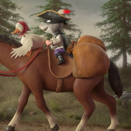
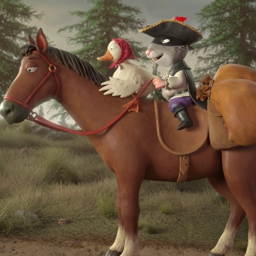
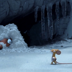
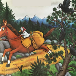
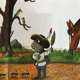
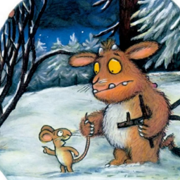
BP

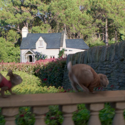
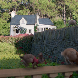
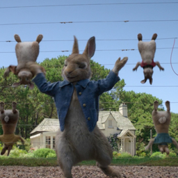
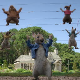
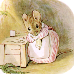
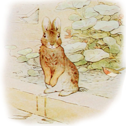
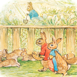
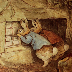
Figure 3: Examples from illustration dataset. On the left, we show sequences from animation movies for AS and BP where temporal relation exists. On the right we show images taken from illustration books and where there is no temporal relation. Also, note that even if the same characters are present in both animations and illustrations, their resemblance is limited. Finally, on BP dataset, for some illustrations there are some small empty areas on the corners of the illustrations.

OpticalFlowWarp: To compare our approach with optical flow based methods we implemented the method in  [34], which will be referred to as OpticalFlowWarp. We calculated optical flows offline and used these pre-computed flows during training. Similar to CycleGANTemp model, we use two frames for the source domain, except they are selected consecutively hence the $\delta$ is fixed to $+1$ for this model. After reference and auxiliary frames are forwarded from $G_{X}$, we warp $x_{t+1}^{{}^{\prime}}$ with the optical flow $F(x_{t},x_{t+1})$ to get the warped version of $x_{t}^{{}^{\prime}}$. We expect the warped stylized frame and the reference stylized frame to be identical. We use $\ell_{1}$ distance between $x_{t}$ and warped frame as the temporal consistency loss;

$$\mathcal{L}_{flow}(x_{t},x_{t+1})=\sum_{i}\|(x_{i}^{{}^{\prime}}-W(x_{i+1}^{{}^{\prime}},F(x_{t+1},x_{t}))\|$$

ReCycleGAN: Our final baselines are ReCycleGAN [11] and its variant adopted to our target domain. ReCycleGAN is a strong baseline for video-to-video translation problems. It integrates a temporal prediction module to capture relations between consecutive frames. However, it assumes that there is a temporal relation both in the source and the target domains. There is almost no temporal relation between the images (i.e. illustrations) taken from the same book. For a fair comparison of ReCycleGAN with our model, we made modifications and created another version of it. We removed all temporal losses on the target domain but kept cyclic losses. We refer to this model as ReCycleGANv2.

III-B WAIT

To capture temporal relations, our model eliminates the requirement for any auxiliary networks such as optical flow or temporal prediction networks. Instead, it warps features extracted from auxiliary frame and reference frame into a single network to generate temporally stable and stylized frames (see Figure 1).

In Figure 2, we present the detailed description of the generator network of WAIT. We use the CycleGAN network without the last convolution layer as the backbone CNN to extract $H\times W\times C$ dimensional features for reference frame $I_{t}$ at time t and a nearby auxiliary frame ($I_{t+\delta}$) at time $\textit{t}+\delta$ where $\delta$ is randomly picked from the set $\{-2,...,+2\}$, respectively. Then, we calculate the difference of these feature maps $\Delta_{F}=I_{t}-I_{t+\delta}$. This difference map is fed to the Offset Network which consists of eight convolutional blocks where each block is composed of two sequences of a $3\times 3$ convolution layer, an Instance Norm [46] and a ReLU layer. These blocks are used to extract offset features. After offset features are calculated, five parallel Warping Layers are used to warp the auxiliary frame $I_{t+\delta}$ with offset features to generate a stylized version of the input frame $I_{t}$. A warping layer consists of a dilated convolution and a deformable convolution layer. Dilated and deformable convolution layers have $3\times 3$ kernels. When we consider a single warping layer, the offset features are first fed to a dilated convolution filter. The outputs of dilated convolution filter is used as offset values of deformable convolution layer and the auxiliary frame is fed to this deformable layer. We use five separate warping layers to capture offset features in different resolutions with increasing dilation values from $3$ to $24$. In the final stage, outputs of each deformable layer are stacked and then a final convolution layer with $7\times 7$ kernels is followed by Tanh activation to generate stylized image.

Only the source domain contains temporal relations. We didn’t observe any improvements using warping layers for both generators in our experiments. Therefore, in our model only $G_{X}$ contains warping layers and $G_{Y}$ contains backbone CNN with final convolution layer i.e. the same network in CycleGAN [1]. Since WAIT model outputs a single stylized image, we use the same training strategy and loss functions as in CycleGAN.

TABLE I: Stats of the datasets used in experiments.

Dataset	Train Frame Cnt		Test Frame Cnt
	Source (Animation)	Target (Illustration)	Source	Target
Axel Scheffler (AS)	9854	551	1475	20
Beatrix Potter (BP)	5560	489	1367	20
Flowers	2067	3270	700	1100

IV Datasets

In our experiments, we have chosen examples from two illustrators: Beatrix Potter (BP) and Axel Scheffler (AS). They have distinct styles and their books are adapted to the animation movies. We have constructed two main datasets, BP and AS, named using the initials of the illustrators. In both datasets, the frames of the animation movies are the source domain and the illustrations of books are the target domain.

BP source split contains Peter Rabbit animation movie. AS source split contains the following animation movies; The Room on the Broom, Stickman, The Gruffalo, The Gruffalo’s Child, The Highway Rat, The Snail and the Whale, and Zog. Due to the large number of frames in AS movies, we select every 30th frame of AS movies while selecting every 10th frame of BP movies. For the illustration dataset, we use illustrations of BP and AS from the dataset presented in [3]. Table I shows number of images in train and test sets. We show some example images for both datasets in Figure 3.

To show the generalization capability of our method to other domains, we also use publicly available Flowers dataset which is presented in [11]. This dataset contains time lapse videos of blooming of different flower species. We use the Dandelion subset which contains 2067 source and 3279 target images for training, and 700 and 1100 images for testing.

Input	CycleGAN	OpticalFlowWarp	ReCycleGAN	ReCycleGANv2	WAIT
[loop,autoplay,width=4cm]5./figures/results_gif/AS/input5/input5-019	[loop,autoplay,width=4cm]5./figures/results_gif/AS/cyclegan5/cyclegan5-019	[loop,autoplay,width=4cm]5./figures/results_gif/AS/optflow5/optflow5-019	[loop,autoplay,width=4cm]5./figures/results_gif/AS/recyclegan5/recyclegan5-019	[loop,autoplay,width=4cm]5./figures/results_gif/AS/recyclegann5/recyclegann5-019	[loop,autoplay,width=4cm]5./figures/results_gif/AS/warp_new5/warp_new5-019
[loop,autoplay,width=4cm]5./figures/results_gif/AS/input4/input4-016	[loop,autoplay,width=4cm]5./figures/results_gif/AS/cyclegan4/cyclegan4-016	[loop,autoplay,width=4cm]5./figures/results_gif/AS/optflow4/optflow4-016	[loop,autoplay,width=4cm]5./figures/results_gif/AS/recyclegan4/recyclegan4-016	[loop,autoplay,width=4cm]5./figures/results_gif/AS/recyclegann4/recyclegann4-016	[loop,autoplay,width=4cm]5./figures/results_gif/AS/warp_new4/warp_new4-016

Figure 4: Visual results on AS dataset. Top row displays a short sequence and on the bottom a long sequence from our test set. Left most column contains the input videos and the following rows correspond to results of baseline methods and WAIT. First of all, for both sequences only WAIT captures target style correctly. In terms of visual quality and temporal coherency, on the first sequence red and black patches on the mouth of the horse are visible for every baseline. On the bottom sequence, the success of WAIT is more visible. For the CycleGAN, OpticalFlowWarp and ReCycleGAN results, it is very obvious that the temporal coherency is not captured. Especially, the color of the background grass and air changes between frames. Also, there are white/black patches/holes moving across the scene for baselines. The quality of the generated frames and temporal coherency between them are very visible for the results of WAIT. Zoom in for details.

V Experiments

V-A Implementation Details

We used PyTorch [47] to implement our models. As in other unpaired video-to-video transfer settings, our method does not need paired frames. Two different image datasets, one for source and the other for target, are used in our model. All training images (i.e. animation frames and illustrations) are resized to $256\times 256$ pixels. We train our models for 200 epoch using Adam solver with a learning rate of 0.0008 and batch size of 8. All networks were trained from scratch. We conducted all of our experiments on Nvidia Tesla A100 GPUs. Our code, pretrained models and the scripts that reproduce the datasets can be found at https://github.com/giddyyupp/wait.

Input	CycleGAN	OpticalFlowWarp	ReCycleGAN	ReCycleGANv2	WAIT
[loop,autoplay,width=4cm]5./figures/results_gif/BP/input3/input3-04	[loop,autoplay,width=4cm]5./figures/results_gif/BP/cyclegan3/cyclegan3-04	[loop,autoplay,width=4cm]5./figures/results_gif/BP/optflow3/optflow3-04	[loop,autoplay,width=4cm]5./figures/results_gif/BP/recyclegan3/recyclegan3-04	[loop,autoplay,width=4cm]5./figures/results_gif/BP/recyclegann3/recyclegann3-04	[loop,autoplay,width=4cm]5./figures/results_gif/BP/warp3/warp3-04
[loop,autoplay,width=4cm]5./figures/results_gif/BP/input2/input2-023	[loop,autoplay,width=4cm]5./figures/results_gif/BP/cyclegan2/cyclegan2-023	[loop,autoplay,width=4cm]5./figures/results_gif/BP/optflow2/optflow2-023	[loop,autoplay,width=4cm]5./figures/results_gif/BP/recyclegan2/recyclegan2-023	[loop,autoplay,width=4cm]5./figures/results_gif/BP/recyclegann2/recyclegann2-023	[loop,autoplay,width=4cm]5./figures/results_gif/BP/warp2/warp2-023

Figure 5: Visual results on BP dataset. We display a short sequence on the top row, and a long sequence at the bottom row from our test set. Left most column contains the input videos and the following rows correspond to results of baseline methods and WAIT. First of all, similar to AS results, for both sequences only WAIT captures the target style correctly. In terms of visual quality and temporal coherency, for the first sequence, colors of the leaves and background changes abruptly for CycleGAN, OpticalFlowWarp and ReCycleGANv2 results. For ReCycleGAN results, there is a white patch on the apple for some frames. On the bottom sequence which is a 5 second clip, the success of WAIT is easy to catch. The style is correctly captured and the temporal coherency is ensured. For the baselines, strangely CycleGAN captures the temporal coherency much better than others. The only defect in CycleGAN results is the pinkish colorization on the wall and the head of the rabbit. For the rest, it is very obvious that the temporal coherency is not captured. The general color palette of the scene changes dramatically between frames. Also, there are white patches/holes on the pumpkin for ReCycleGANv2 results. Zoom in for details.

V-B Qualitative Analysis

In Figure 4, we show example sequences from the test set of AS and compare the results of baseline methods and our method visually. On the top row, we present results for a short clip (1.5 sec.) and on the second row for a longer clip (3 sec.). For both sequences, all baseline methods except OpticalFlowWarp, generate visually plausible results. However, the baseline methods fail to capture the style of the illustrator, and/or lack temporal coherence. Moreover, especially for the second sequence, where we display frames from a 3 seconds clip, patches arise there around objects with the baseline methods. For instance, on ReCycleGAN and ReCycleGANv2 results dark patches exist on the mouse, tail of the horse or both. These visual results align with the FID results. Mode collapsed OpticalFlowWarp model has the highest FID and its visual results are the worst compared to other baselines. On the contrary, WAIT captured both temporal coherence and target style at the same time.

Visual results for the BP dataset are presented in Figure 5. Similar to AS results, on the top row we present results for a short clip (1 sec.) and on the second row for a longer clip (5 sec.). Flickering effects are easily visible on the results of the baseline methods. Colors are not consistent across the consecutive frames. For instance, on the second sequence rocks on the background become pinkish starting from the first frame on CycleGAN results. For OpticalFlowWarp, ReCycleGAN and ReCycleGANv2, intensity of colors changed on the second and the third frames. On the other hand, our model gave both correctly stylized and consistent results.

V-C Quantitative Analysis

There are two aspects for a successful video translation: visual similarity of the translated images to the target domain and the temporal stability between stylized frames. To quantitatively evaluate the quality of video translation in terms of both aspects, we use three metrics.

TABLE II: Results on the AS dataset. Lower is better for all metrics. Best results for each metric are boldfaced. ^† indicates that results are not reliable, since the model failed to converge. Our method achieves best score on FID and FWE metrics, and competitive result on MSE metric.

Method	Metrics
	FID	FWE	MSE
CycleGAN [1]	175.25	0.006325	8528.95
OpticalFlowWarp [30]	$205.69^{\dagger}$	$0.001747^{\dagger}$	$4566.95^{\dagger}$
ReCycleGAN [11]	177.59	0.003580	4397.43
ReCyleGANv2	177.16	0.003284	4395.39
CycleGANTemp	165.70	0.004998	7197.36
WAIT	164.06	0.003245	4928.44

Fréchet Inception Distance (FID) [48] is a widely used metric to evaluate visual similarity between two domains. FID compares the distributions of the features of generated and real images and calculates the distance between them. Lower FID score yields higher visual similarity. First, real and generated images are fed to a CNN model (e.g. Inception [49] or VGG [50]) trained on ImageNet [51] with the classifier part removed, and activations are extracted for both domains ($X_{r}$ and $X_{f}$). Then, mean ($m_{r}$ and $m_{f}$) and covariance ($C_{r}$ and $C_{f}$) statistics are calculated from the activations of both domains separately. Final FID score is the sum of the squared distance between mean values and trace of the covariance matrices:

$$FID=\|m_{r}-m_{f}\|^{2}+tr(C_{r}+C_{f}-2\times(C_{r}\times C_{f})^{1/2})$$

In order to measure temporal coherency, we use flow warping error (FWE) [19, 30] and mean squared error (MSE) [13] metrics.

The Flow Warping Error (FWE) computes the average pixel-wise Euclidean color difference between consecutive frames:

$$FWE=\frac{1}{T-1}\sum_{t=1}^{T-1}\sum_{i,j,c}M_{i,j}\times\|y_{t}^{i,j,c}-\hat{y_{t}}^{i,j,c}\|_{2}^{2}$$

where $y_{t}$ is the stylized framed at time $t$, $\hat{y_{t}}$ is the warped frame at time $t$ and which is calculated as $\hat{y_{t}}=W({y_{t}},f(x_{t-1},x_{t}))$. $M_{i,j}$ is a non-occlusion mask at location $i,j$ indicating non-occluded regions. We follow [13] and use the occlusion detection method in [18] to estimate the $M$. The $W$ function refers to flow warping operation using stylized frame $y_{t}$ and optical flow $f$ calculated between input frames $x_{t-1}$ and $x_{t}$.

TABLE III: Results on the BP dataset. Lower is better for all metrics. Best results for each metric are boldfaced. Our method achieves best score on FID and FWE metrics, and competitive result on MSE metric.

Method	Metrics
	FID	FWE	MSE
CycleGAN [1]	192.55	0.007519	10682.98
OpticalFlowWarp [30]	166.68	0.003850	6737.55
ReCycleGAN [11]	172.78	0.003781	6493.49
ReCyleGANv2	170.01	0.003780	6896.81
CycleGANTemp	165.70	0.003998	7197.36
WAIT	160.09	0.003717	6745.54

TABLE IV: Results on the Flowers dataset. Lower is better for all metrics. Best results for each metric are boldfaced. Our method achieves best score on FID metric.

Method	Metrics
	FID	FWE	MSE
CycleGAN [1]	184.49	0.000246	1153.57
OpticalFlowWarp [30]	265.94	0.001381	3691.79
ReCycleGAN [11]	333.53	0.002080	5257.71
ReCyleGANv2	329.17	0.001366	4698.50
CycleGANTemp	178.98	0.001718	4694.23
WAIT	165.55	0.001136	3823.15

The Mean Squared Error (MSE) measures the errors between color difference of consecutive frames in both input and generated images:

$$MSE={}\frac{1}{T-1}\sum_{t=1}^{T-1}\sum_{i,j,c} \|(x_{t+1}^{i,j,c}-x_{t}^{i,j,c})-$$

$$({y_{t+1}}^{i,j,c}-{y_{t}}^{i,j,c})\|_{2}^{2}$$

where $x_{t}$ and $x_{t+1}$ are two consecutive frames in the source domain, and $y_{t}$ and $y_{t+1}$ are corresponding stylized frames.

We present FID, FWE and MSE results for baseline models and our WAIT model in Table II and Table III for AS and BP datasets, respectively. On all datasets, our method performs significantly better than CycleGAN and ReCyleGAN, which shows the effectiveness of our method. Specifically on the AS dataset, our method improves baseline CycleGAN by 11 points on FID. Also, it reduces FWE and MSE metrics by almost 50% and 40% respectively. Similarly on the BP dataset, FID score is improved by 32 points compared to CycleGAN. Moreover, FWE and MSE metrics are also significantly improved. Compared to ReCycleGAN, both methods achieve similar performances regarding temporal consistency metrics which shows that our model captures temporal relations with a much simpler design. On the other hand, our model’s visual quality performance is much better than ReCycleGAN. Also, our modified version of ReCycleGAN performs slightly better than the original as expected. One final remark is that our simple baseline “CycleGANTemp" model performs quite well.

In Table IV, we present results on Flowers dataset. This dataset contains temporal relation on both source and target domains. Our model performed the best in terms of FID scores. However, CycleGAN outperformed others on FWE and MSE metrics. The main reason for that is that the Flowers dataset is a very simple dataset that contains a fixed background and the main action happens in a very small, fixed area. FWE and MSE scores are very low for every model compared to illustration dataset results.

TABLE V: Comparison of methods in terms of train and test run times in minutes on a single Nvidia A100 GPU.

Method	Phase
	Train	Test
CycleGAN [1]	16	59
OpticalFlowWarp [30]	21.4	59
ReCycleGAN [11]	19.6	96
ReCyleGANv2	13.8	62
CycleGANTemp	29.4	69
WAIT	18.8	54

In Table V, we compare all the models in terms of training and testing run times. Regarding training time we measure training a single epoch using AS dataset on a single Nvidia V100 GPU. And for testing time, we measure total time to test the Flowers dataset (including measuring the metrics) on the same GPU. For optical flow warping model, we calculated the flows offline for both train and test sets and used these pre-computed flows during training and testing. Optical flow warping models generally calculate optical flows during training on the fly to be able to randomly define the stride between selected frames. For training, our modified light version of ReCycleGAN got the smallest time. WAIT sits between the baseline CycleGAN and Flow Warping model. For test time, except ReCycleGAN all models have similar numbers since they all use a single frame to generate stylized images.

TABLE VI: Ablation experiments for the WAIT model. (a) Effect of the depth of offset network layers on performance. Offset network with $8$ residual blocks has the best performance. (b) Effect of parallel warping layers. Here, the depth of the offset network is $8$ residual blocks and the time gap is $2$. Using $5$ warping layers gave the best performance. (c) Effect of time gap. Offset Network depth is $8$ and the number of Warping layers is $5$. Using $2$ as time gap yields the best result.

Param.	FID	FWE	MSE
6	259.79	0.008790	15623.18
8	160.09	0.003717	6745.54
10	271.41	0.011621	15699.60
(a) Effect of Offset Network Depth
1	291.73	0.019609	20976.54
2	253.89	0.013174	15397.60
3	279.42	0.006250	12571.42
4	299.17	0.013147	16323.93
5	160.09	0.003717	6745.54
(b) Effect of Warping Layer Number
1	174.45	0.005270	8116.54
2	160.09	0.003717	6745.54
3	177.37	0.004241	7583.23
4	220.92	0.018734	17913.86
5	154.94	0.005571	8564.26
(c) Varying Time Gap

V-D Ablation Experiments

In order to evaluate the effects of different parts of our model and time gap parameter during training in detail, we conducted three ablation experiments. Our model consists of three main blocks, Backbone CNN, Offset Network and Warping Layers. Our Backbone CNN is amongst the established architectures for style transfer and used by many previous works such as CycleGAN [1] and ReCycleGAN [11]. Offset Network and Warping Layers are two critical parts of the model, so in our ablation experiments, we focused on these two parts. We performed all ablations on the BP dataset. We trained models for $300$ epochs with a batch size of $8$.

Offset Network. We conducted ablation experiments to set the depth of the Offset Network. We used depth values of $6$, $8$ and $10$. In all these experiments, we fixed the Warping layer number to $5$ and the time gap value to $2$. Results are presented in Table VIa. We obtained the best performance on all metrics with depth value of $8$.

Warping Layer. Warping layer warps auxiliary features with offset features with different resolutions. To decide how many warping layers we should integrate in our network, we perform experiments by increasing the warping layer number from $1$ to $5$. We fixed the depth of Offset Network as $8$ and time gap value to $2$ in these ablations. In Table VIb, we present results of these experiments. Using $5$ parallel warping layers gave the best performance considering all three metrics. Although, adding more warping layers increases the performance, it also slows down the training and testing times. So, we choose $5$ parallel warping layers in the final model.

Time Gap. Finally, in order to determine the optimum time difference between reference and auxiliary frames, we experimented with values in the range of $1$ to $5$. Using $2$ as time gap parameter performed the best regarding temporal metrics. Results are given in Table VIc.

VI Conclusions

In this paper, we propose a new method for video-to-video translation. Our method removes the need of additional networks e.g. optical flow or temporal predictors to ensure temporal coherency between translated frames. We validated our method on a new challenging task, translating animation movies to their illustration versions. Our method achieved the best scores on FID and FWE metrics compared to current state-of-the-art methods. We conducted extensive ablations to analyze different parts of our model.

VII Acknowledgements

The numerical calculations reported in this paper were fully performed at TUBITAK ULAKBIM, High Performance and Grid Computing Center (TRUBA resources).

References

- [1] J.-Y. Zhu, T. Park, P. Isola, and A. A. Efros, “Unpaired image-to-image translation using cycle-consistent adversarial networks,” IEEE International Conference on Computer Vision, 2017.
- [2] P. Isola, J.-Y. Zhu, T. Zhou, and A. A. Efros, “Image-to-image translation with conditional adversarial networks,” IEEE Conference on Computer Vision and Pattern Recognition, 2017.
- [3] S. Hicsonmez, N. Samet, E. Akbas, and P. Duygulu, “Ganilla: Generative adversarial networks for image to illustration translation,” Image and Vision Computing, 2020.
- [4] Y. Chen, Y.-K. Lai, and Y.-J. Liu, “Cartoongan: Generative adversarial networks for photo cartoonization,” in IEEE Conference on Computer Vision and Pattern Recognition, 2018.
- [5] Z. Yi, H. Zhang, P. Tan, and M. Gong, “Dualgan: Unsupervised dual learning for image-to-image translation,” IEEE International Conference on Computer Vision, 2017.
- [6] L. A. Gatys, A. S. Ecker, and M. Bethge, “A neural algorithm of artistic style,” arXiv preprint arXiv:1508.06576, 2015.
- [7] ——, “Image style transfer using convolutional neural networks,” IEEE Conference on Computer Vision and Pattern Recognition, 2016.
- [8] X. Huang, M.-Y. Liu, S. Belongie, and J. Kautz, “Multimodal unsupervised image-to-image translation,” in IEEE European Conference on Computer Vision, 2018, pp. 172–189.
- [9] M.-Y. Liu, T. Breuel, and J. Kautz, “Unsupervised image-to-image translation networks,” in Advances in Neural Information Processing Systems, 2017, pp. 700–708.
- [10] D. Chen, J. Liao, L. Yuan, N. Yu, and G. Hua, “Coherent online video style transfer,” in IEEE International Conference on Computer Vision, 2017, pp. 1105–1114.
- [11] A. Bansal, S. Ma, D. Ramanan, and Y. Sheikh, “Recycle-gan: Unsupervised video retargeting,” in IEEE European Conference on Computer Vision, 2018, pp. 119–135.
- [12] Y. Chen, Y. Pan, T. Yao, X. Tian, and T. Mei, “Mocycle-gan: Unpaired video-to-video translation,” in ACM International Conference on Multimedia, 2019, pp. 647–655.
- [13] K. Xu, L. Wen, G. Li, H. Qi, L. Bo, and Q. Huang, “Learning self-supervised space-time cnn for fast video style transfer,” IEEE Transactions on Image Processing, vol. 30, pp. 2501–2512, 2021.
- [14] T.-C. Wang, M.-Y. Liu, J.-Y. Zhu, G. Liu, A. Tao, J. Kautz, and B. Catanzaro, “Video-to-video synthesis,” in Advances in Neural Information Processing Systems, 2018.
- [15] X. Chen, Y. Zhang, Y. Wang, H. Shu, C. Xu, and C. Xu, “Optical flow distillation: Towards efficient and stable video style transfer,” in IEEE European Conference on Computer Vision. Springer, 2020, pp. 614–630.
- [16] K. Liu, S. Gu, A. Romero, and R. Timofte, “Unsupervised multimodal video-to-video translation via self-supervised learning,” in Winter Conference on Applications of Computer Vision, 2021, pp. 1030–1040.
- [17] C. Gao, D. Gu, F. Zhang, and Y. Yu, “Reconet: Real-time coherent video style transfer network,” in Asian Conference on Computer Vision. Springer, 2018, pp. 637–653.
- [18] M. Ruder, A. Dosovitskiy, and T. Brox, “Artistic style transfer for videos and spherical images,” International Journal of Computer Vision, pp. 1199–1219, 2018.
- [19] H. Huang, H. Wang, W. Luo, L. Ma, W. Jiang, X. Zhu, Z. Li, and W. Liu, “Real-time neural style transfer for videos,” in IEEE Conference on Computer Vision and Pattern Recognition, 2017, pp. 783–791.
- [20] W. Gao, Y. Li, Y. Yin, and M.-H. Yang, “Fast video multi-style transfer,” in Winter Conference on Applications of Computer Vision, 2020, pp. 3222–3230.
- [21] A. Gupta, J. Johnson, A. Alahi, and L. Fei-Fei, “Characterizing and improving stability in neural style transfer,” in IEEE International Conference on Computer Vision, 2017, pp. 4067–4076.
- [22] W. Wang, J. Xu, L. Zhang, Y. Wang, and J. Liu, “Consistent video style transfer via compound regularization,” in AAAI Conference on Artificial Intelligence, vol. 34, no. 07, 2020, pp. 12 233–12 240.
- [23] N. Mayer, E. Ilg, P. Hausser, P. Fischer, D. Cremers, A. Dosovitskiy, and T. Brox, “A large dataset to train convolutional networks for disparity, optical flow, and scene flow estimation,” in IEEE Conference on Computer Vision and Pattern Recognition, 2016.
- [24] A. Dosovitskiy, P. Fischer, E. Ilg, P. Hausser, C. Hazirbas, V. Golkov, P. Van Der Smagt, D. Cremers, and T. Brox, “Flownet: Learning optical flow with convolutional networks,” in IEEE International Conference on Computer Vision, 2015, pp. 2758–2766.
- [25] X. Li, S. Liu, J. Kautz, and M.-H. Yang, “Learning linear transformations for fast image and video style transfer,” in IEEE Conference on Computer Vision and Pattern Recognition, 2019, pp. 3809–3817.
- [26] G. Bertasius and L. Torresani, “Classifying, segmenting, and tracking object instances in video with mask propagation,” in IEEE Conference on Computer Vision and Pattern Recognition, June 2020.
- [27] J. Wu, J. Cao, L. Song, Y. Wang, M. Yang, and J. Yuan, “Track to detect and segment: An online multi-object tracker,” in IEEE Conference on Computer Vision and Pattern Recognition, 2021, pp. 12 352–12 361.
- [28] U. Rafi, A. Doering, B. Leibe, and J. Gall, “Self-supervised keypoint correspondences for multi-person pose estimation and tracking in videos,” in IEEE European Conference on Computer Vision. Springer, 2020, pp. 36–52.
- [29] G. Bertasius, C. Feichtenhofer, D. Tran, J. Shi, and L. Torresani, “Learning temporal pose estimation from sparsely-labeled videos,” Advances in Neural Information Processing Systems, vol. 32, 2019.
- [30] W.-S. Lai, J.-B. Huang, O. Wang, E. Shechtman, E. Yumer, and M.-H. Yang, “Learning blind video temporal consistency,” in IEEE European Conference on Computer Vision, 2018, pp. 170–185.
- [31] T.-C. Wang, M.-Y. Liu, J.-Y. Zhu, A. Tao, J. Kautz, and B. Catanzaro, “High-resolution image synthesis and semantic manipulation with conditional gans,” in IEEE Conference on Computer Vision and Pattern Recognition, 2018, pp. 8798–8807.
- [32] T. Kim, M. Cha, H. Kim, J. K. Lee, and J. Kim, “Learning to discover cross-domain relations with generative adversarial networks,” CoRR, vol. abs/1703.05192, 2017.
- [33] Y. Choi, M. Choi, M. Kim, J.-W. Ha, S. Kim, and J. Choo, “Stargan: Unified generative adversarial networks for multi-domain image-to-image translation,” in IEEE Conference on Computer Vision and Pattern Recognition, 2018, pp. 8789–8797.
- [34] M. Ruder, A. Dosovitskiy, and T. Brox, “Artistic style transfer for videos,” in German conference on pattern recognition. Springer, 2016, pp. 26–36.
- [35] X. Wei, J. Zhu, S. Feng, and H. Su, “Video-to-video translation with global temporal consistency,” in ACM International Conference on Multimedia, 2018, pp. 18–25.
- [36] T.-C. Wang, M.-Y. Liu, A. Tao, G. Liu, J. Kautz, and B. Catanzaro, “Few-shot video-to-video synthesis,” in Advances in Neural Information Processing Systems, 2019.
- [37] K. Park, S. Woo, D. Kim, D. Cho, and I. S. Kweon, “Preserving semantic and temporal consistency for unpaired video-to-video translation,” in ACM International Conference on Multimedia, 2019, pp. 1248–1257.
- [38] O. Frigo, N. Sabater, J. Delon, and P. Hellier, “Video style transfer by consistent adaptive patch sampling,” The Visual Computer, vol. 35, no. 3, pp. 429–443, 2019.
- [39] A. Mallya, T.-C. Wang, K. Sapra, and M.-Y. Liu, “World-consistent video-to-video synthesis,” in IEEE European Conference on Computer Vision, 2020.
- [40] O. Texler, D. Futschik, M. Kučera, O. Jamriška, Š. Sochorová, M. Chai, S. Tulyakov, and D. Sỳkora, “Interactive video stylization using few-shot patch-based training,” ACM Transactions on Graphics (TOG), vol. 39, no. 4, pp. 73–1, 2020.
- [41] W. Wang, S. Yang, J. Xu, and J. Liu, “Consistent video style transfer via relaxation and regularization,” IEEE Transactions on Image Processing, vol. 29, pp. 9125–9139, 2020.
- [42] S. Liu and T. Zhu, “Structure-guided arbitrary style transfer for artistic image and video,” IEEE Transactions on Multimedia, 2021.
- [43] E. Ilg, N. Mayer, T. Saikia, M. Keuper, A. Dosovitskiy, and T. Brox, “Flownet 2.0: Evolution of optical flow estimation with deep networks,” in IEEE Conference on Computer Vision and Pattern Recognition, 2017.
- [44] H. Liu, C. Li, D. Lei, and Q. Zhu, “Unsupervised video-to-video translation with preservation of frame modification tendency,” The Visual Computer, vol. 36, no. 10, pp. 2105–2116, 2020.
- [45] D. Bashkirova, B. Usman, and K. Saenko, “Unsupervised video-to-video translation,” arXiv preprint arXiv:1806.03698, 2018.
- [46] D. Ulyanov, A. Vedaldi, and V. S. Lempitsky, “Instance normalization: The missing ingredient for fast stylization,” CoRR, vol. abs/1607.08022, 2016.
- [47] A. Paszke, S. Gross, S. Chintala, G. Chanan, E. Yang, Z. DeVito, Z. Lin, A. Desmaison, L. Antiga, and A. Lerer, “Automatic differentiation in pytorch,” 2017.
- [48] M. Heusel, H. Ramsauer, T. Unterthiner, B. Nessler, and S. Hochreiter, “Gans trained by a two time-scale update rule converge to a local nash equilibrium,” in Advances in Neural Information Processing Systems, 2017, pp. 6626–6637.
- [49] C. Szegedy, V. Vanhoucke, S. Ioffe, J. Shlens, and Z. Wojna, “Rethinking the inception architecture for computer vision,” in IEEE Conference on Computer Vision and Pattern Recognition, 2016, pp. 2818–2826.
- [50] K. Simonyan and A. Zisserman, “Very deep convolutional networks for large-scale image recognition,” 2014.
- [51] J. Deng, W. Dong, R. Socher, L.-J. Li, K. Li, and L. Fei-Fei, “Imagenet: A large-scale hierarchical image database,” in IEEE Conference on Computer Vision and Pattern Recognition, 2009, pp. 248–255.