Scalar bosons in Bonnor-Melvin-$\Lambda$ universe: Exact solution, Landau levels and Coulomb-like potential

Abstract

In this work we study spin-0 particles in a spacetime which structure is determined by a homogeneous magnetic field and a cosmological constant. For this purpose we take into account a framework based on the Bonnor-Melvin solution with the inclusion of the cosmological constant. We write the Klein-Gordon equation, solve it and determine the Landau levels. The effect of a scalar potential is also considered.

1 Introduction

Probably one of the most intriguing theories in physics is the general theory of relativity. As far as it describes the gravitational interaction in terms of the geometry of the spacetime many unexpected effects have been discovered as for example the Lense-Thirring effect [1], [2], that deals with the frame dragging, gravitational waves [3] or even gravitational lensing [4],[5].

Recently, the interest in studies about magnetic fields has increased as far as many systems with very strong fields have been reported such as magnetars [6], [7] and heavy ion collisions [8], [9], [10]. So, a question of interest is how to incorporate the magnetic field in the general relativity framework.

Currently some solutions of the Einstein-Maxwell equations are known, the Manko solution [11], [12], the Bonnor-Melvin universe [13], [14] and a recently proposed solution [15] based on the Bonnor-Melvin solution with the inclusion of the cosmological constant.

Still thinking about the general relativity, another important aspect is how this theory may be related with the quantum physics, or if this kind of relation may also exist, or at least be relevant. At the moment many works have been proposed with this purpose and are essentially based on the Klein-Gordon and Dirac equations written in curved spacetimes [16], [17]. Typical examples are particles in the Schwarzschild [18], Kerr black holes [19] and in cosmic string [20] , [21], [22] backgrounds, quantum oscillators [23], [24], [25], [26], [27], [28], Casimir effect [29], [30] or particles in the Hartle-Thorne spacetime [31]. These studies and others [32], [33], [34] have provided many interesting results and insights about how quantum systems are affected by arbitrary geometries of the spacetime.

So, an interesting subject is to study of quantum particles in a spacetime with the structure affected by a magnetic field. In [35], Dirac particles have been studied in the Melvin metric. In this work we study spin-0 bosons in the magnetic universe with cosmological constant proposed in [15].

The structure of this paper is as follows: In Sec. II, the Klein-Gordon in the Bonnor-Melvin-$\Lambda$ is obtained and solved. Then the Landau levels are determined. In Sec. III a Coulomb-like potential is introduced and the new equation is solved, and in Sec. IV we draw our conclusions.

2 Klein-Gordon equation in Bonnor-Melvin-$\Lambda$ universe

In order to study quantum particles in a spacetime determined by the influence of a magnetic field we will consider the solution proposed in [15], that is a static solution of the Einstein-Maxwell equations with cylindrical symmetry generated by a homogeneous magnetic field and the inclusion of the cosmological constant, which is given by

$$ds^{2}=-dt^{2}+d\rho^{2}+\sigma^{2}\sin^{2}\left(\sqrt{2\Lambda}\rho\right)d\varphi^{2}+dz^{2},$$ (1)

where $\Lambda$ is the cosmological constant and $\sigma$ is a constant of integration that is related to the magnetic field by the relation

$$H(r)=\sqrt{\Lambda}\sigma\sin\left(\sqrt{2\Lambda}\rho\right).$$ (2)

In this work we consider scalar bosons inside this spacetime which may be described by the Klein-Gordon equation written in curved spaces [17] that is given by

$$\frac{1}{\sqrt{-g}}\partial_{\mu}\left[g^{\mu\nu}\sqrt{-g}\partial_{\nu}\Psi\right]-m^{2}\Psi=0,$$ (3)

that in terms of the line element (1) is

$$\left(-\frac{\partial^{2}}{\partial t^{2}}+\frac{\sqrt{2\Lambda}}{\tan\left(\sqrt{2\Lambda}\rho\right)}\frac{\partial}{\partial\rho}+\frac{\partial^{2}}{\partial\rho^{2}}+\frac{\partial^{2}}{\partial z^{2}}+\frac{1}{\sigma^{2}\sin^{2}\left(\sqrt{2\Lambda}\rho\right)}\frac{\partial^{2}}{\partial\varphi^{2}}-m^{2}\right)\Psi\left(t,\rho,\varphi,z\right)=0.$$ (4)

We should note that equation (4) does not depend on the variables $t$ and $z$, then the solution have the form

$$\Psi\left(t,\rho,\varphi,z\right)=e^{i\epsilon t}e^{il\varphi}e^{ip_{z}z}R\left(\rho\right)$$ (5)

where $\epsilon$, $l$ and $p_{z}$ ara the quantum numbers associated with energy, angular momentum around $\varphi$ and momentum in the $z$ direction respectively, and it remains for us to determine the dynamics of the radial component of the equation. Substituting (5) into (4) and defining

$$\zeta^{2}=\epsilon^{2}-m^{2}-p_{z}^{2}$$ (6)

we get the radial differential equation

$$\frac{d^{2}R\left(\rho\right)}{d\rho^{2}}+\frac{\sqrt{2\Lambda}}{\tan\left(\sqrt{2\Lambda}\rho\right)}\frac{dR\left(\rho\right)}{d\rho}+\left[\zeta^{2}-\frac{l^{2}}{\sigma^{2}\sin^{2}\left(\sqrt{2\Lambda}\rho\right)}\right]R\left(\rho\right)=0$$ (7)

and to solve this equation, we make the following change of variables $u=\cos\left(\sqrt{2\Lambda}\rho\right)$, which results in

$$\left(1-u^{2}\right)\frac{d^{2}R\left(u\right)}{du^{2}}-2u\frac{dR\left(u\right)}{du}+\left(\frac{\zeta^{2}}{2\Lambda}-\frac{1}{\left(1-u^{2}\right)}\frac{l^{2}}{2\Lambda\sigma^{2}}\right)R\left(u\right)=0.$$ (8)

Identifying $\mu\equiv\frac{\left|l\right|}{\sqrt{2\Lambda}\sigma}$ and $\nu\equiv\left(\frac{\zeta^{2}}{2\Lambda}+\frac{1}{4}\right)^{\frac{1}{2}}-\frac{1}{2}$, the equation takes the form of an associated Legendre equation

$$\left(1-u^{2}\right)\frac{d^{2}R\left(u\right)}{du^{2}}-2u\frac{dR\left(u\right)}{du}+\left(\nu\left(\nu+1\right)-\frac{\mu^{2}}{1-u^{2}}\right)R\left(u\right)=0,$$ (9)

whose solutions to $\mu,\nu\in\mathbb{R}$ and $u\in(-1,1)$ are the so-called Ferrer functions of the first and second type [36], which are respectively denoted by $\mathrm{P}_{\nu}^{\mu}\left(u\right)\ \rm{and}\ \mathrm{Q}_{\nu}^{\mu}\left(u\right)$ and for $\mu$ and $\nu$ integers are the usual associated Legendre functions. Since $\mathrm{P}_{\nu}^{\mu}\left(u\right)$ is well defined for any $\mu,\nu$, the solution becomes

$$R\left(u\right)=\mathrm{P}_{\nu}^{\mu}\left(u\right)=\left(\frac{1+x}{1-x}\right)^{\frac{\mu}{2}}\boldsymbol{F}\left(\nu+1,-\nu+1;1-\mu;\frac{1}{2}-\frac{1}{2}u\right),$$ (10)

recovering the parameters, we can write the solution for the radial component

$$R\left(u\right)=\mathrm{P}_{\left(\frac{\zeta^{2}}{2\Lambda}+\frac{1}{4}\right)^{\frac{1}{2}}-\frac{1}{2}}^{\frac{\left|l\right|}{\sqrt{2\Lambda}\sigma}}\left(u\right)=\left(\frac{1+u}{1-u}\right)^{\frac{\left|l\right|}{2\sqrt{2\Lambda}\sigma}}\boldsymbol{F}\left(a,b;c;\frac{1}{2}\left(1-u\right)\right);$$ (11)

such that $a\equiv\left(\frac{\zeta^{2}}{2\Lambda}+\frac{1}{4}\right)^{\frac{1}{2}}+\frac{1}{2}$, $b\equiv-\left(\frac{\zeta^{2}}{2\Lambda}+\frac{1}{4}\right)^{\frac{1}{2}}+\frac{3}{2}$ and $c\equiv 1-\frac{\left|l\right|}{\sqrt{2\Lambda}\sigma}$. Observing the fact that the cosmological constant $\Lambda$ is very small, it implies that $\nu$ is large enough such that in this regime it is worth $\nu=\frac{\zeta}{\sqrt{2\Lambda}}-\frac{1}{2}$. So, it is possible to take the asymptotic expression for the radial solution

$$\mathrm{P}_{\frac{\zeta}{\sqrt{2\Lambda}}-\frac{1}{2}}^{\frac{\left|l\right|}{\sqrt{2\Lambda}\sigma}}\left(\cos\left(\sqrt{2\Lambda}\rho\right)\right)\sim\left(\frac{\sqrt{2\Lambda}\rho}{\sin\left(\sqrt{2\Lambda}\rho\right)}\right)^{\frac{1}{2}}J_{\frac{\left|l\right|}{\sqrt{2\Lambda}\sigma}}\left(\zeta\rho\right)\sim J_{\frac{\left|l\right|}{\sqrt{2\Lambda}\sigma}}\left(\zeta\rho\right),$$ (12)

where $J_{\frac{\left|l\right|}{\sqrt{2\Lambda}\sigma}}\left(\zeta\rho\right)$ is a Bessel function, with a high degree of accuracy.

We may also begin the calculations by assuming that the cosmological constant is small, in this case we can consider a first-order expansion in $\Lambda\rho$ into the components of the metric (1) so that we can write

$$ds^{2}=-dt^{2}+d\rho^{2}+2\Lambda\sigma^{2}\rho^{2}d\varphi^{2}+dz^{2}\ .$$ (13)

Following a procedure similar to the one used in obtaining the radial equation (7), now the equation of interest is given by

$$\frac{d^{2}R\left(\rho\right)}{d\rho^{2}}+\frac{1}{\rho}\frac{dR\left(\rho\right)}{dr}+\left[\zeta^{2}-\frac{l^{2}}{2\Lambda\sigma^{2}\rho^{2}}\right]R\left(\rho\right)=0\ .$$ (14)

Performing the change of variables $\overline{\rho}=\zeta\rho$, the radial equation one more time takes the form of a Bessel equation, whose general solution is expressed in terms of Bessel functions of the first type $J_{\lambda}$ and second type $Y_{\lambda}$, with $\lambda=\frac{l}{\sigma\sqrt{2\Lambda}}$, so the radial component can be written as

$$R\left(\rho\right)=c_{1}J_{\frac{\left|l\right|}{\sigma\sqrt{2\Lambda}}}\left(\zeta\rho\right)+c_{2}Y_{\frac{\left|l\right|}{\sigma\sqrt{2\Lambda}}}\left(\zeta\rho\right).$$ (15)

It turns out that $Y_{\lambda}$ diverges at the origin and therefore, we take $c_{2}=0$, which shows consistency between the approximation made and the asymptotic treatment of the exact solution shown in eq. (12).

2.1 Landau levels

In order to determine the energy spectrum, we can impose the hard-wall boundary condition in the same way it has been proposed in [37, 38], which consists in assuming that the wave function vanishes at some $\rho=\rho_{\omega}$ which is an arbitrary radius and far from the origin. The energy levels may be obtained in terms of the roots of the Bessel functions by the relation

$$J_{\frac{\left|l\right|}{\sqrt{2\Lambda}\sigma}}\left(\zeta\rho_{\omega}\right)=0,$$ (16)

that means that $\zeta\rho_{\omega}$ are the roots of the given Bessel function. A solution easier to handle may be found by using the asymptotic expansion of the Bessel function

$$J_{\frac{\left|l\right|}{\sqrt{2\Lambda}\sigma}}\left(\zeta\rho\right)\sim\sqrt{\frac{2}{\pi\zeta\rho}}\cos\left(\zeta\rho-\frac{\left|l\right|}{\sqrt{2\Lambda}\sigma}\frac{\pi}{2}-\frac{\pi}{4}\right),$$ (17)

imposing the hard wall condition in this expression and considering that the cosine function is periodic we obtain

$$\zeta\rho_{\omega}-\frac{\left|l\right|}{\sqrt{2\Lambda}\sigma}\frac{\pi}{2}-\frac{\pi}{4}=\frac{\pi}{2}+n\pi,$$ (18)

where $n$ is an integer. Remembering the definition $\zeta^{2}=\epsilon^{2}-m^{2}-p_{z}^{2}$, we may determine the energy spectrum

$$\epsilon=\sqrt{\left[\left(\frac{3}{4}+n\right)^{2}+\left(\frac{3}{4}+n\right)\frac{\left|l\right|}{\sqrt{2\Lambda}\sigma}+\frac{l^{2}}{8\Lambda\sigma^{2}}\right]\frac{\pi^{2}}{\rho_{\omega}^{2}}+m^{2}+p_{z}^{2}}$$ (19)

Figures 1 and 2 show some of these levels from eq. (19) using the $\pi^{0}$ as a test particle with mass $m$=0.135 GeV [39], $p_{z}=\rho_{\omega}^{-1}=m$, and a magnetic field with intensity $H_{0}=\sqrt{2\Lambda}\sigma$=$10^{19}$G, that is a value compatible with some estimates for the fields produced in high energy heavy ion collisions [8]. In Figures 3 and 4 we keep the same parameters and only change the value $\rho_{\omega}^{-1}=0.0135$ GeV. In these figures we may see the general behavior of the landau levels for the given set of parameters.

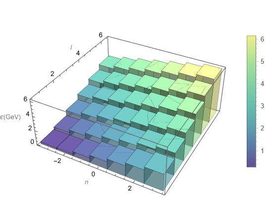
Figure 1: Graph of the energy spectrum in GeV, for $n$ ranging from $-3$ to $3$ and $l$ ranging from $1$ to $6$. In natural units, $p_{z}=m=0.135$ GeV and $\rho_{\omega}^{-1}=0.135$ GeV.

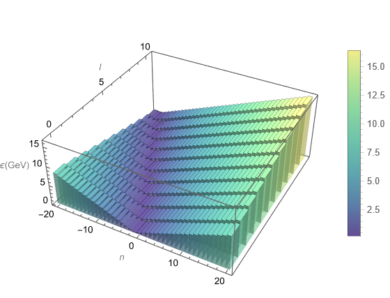
Figure 2: Graph of the energy spectrum in GeV, for $n$ ranging from $-20$ to $20$ and $l$ ranging from $0$ to $20$. In natural units, $p_{z}=m=0.135$ GeV and $\rho_{\omega}^{-1}=0.135$ GeV.

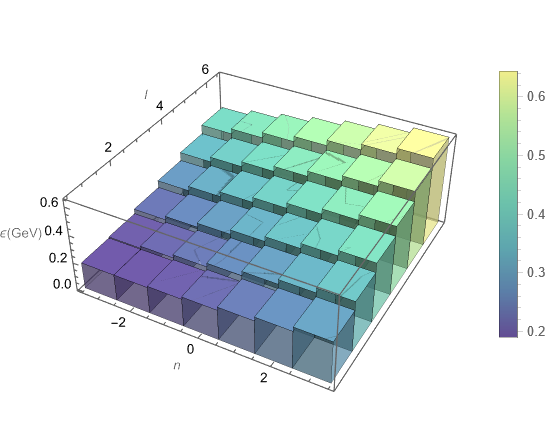
Figure 3: Graph of the energy spectrum in GeV, for $n$ ranging from $-3$ to $3$ and $l$ ranging from $1$ to $6$. In natural units, $p_{z}\sim m=0.135$ GeV and $\rho_{\omega}^{-1}=0.0135$ GeV.

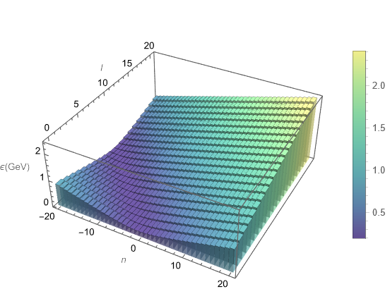
Figure 4: Graph of the energy spectrum in GeV, for $n$ ranging from $-20$ to $20$ and $l$ ranging from $0$ to $20$. In natural units, $p_{z}=m=0.134$ GeV and $\rho_{\omega}^{-1}=0.0135$ GeV.

3 Coulomb-like potential

Another interesting system that may be studied in a similar way is the spin-0 bosons in the presence of a scalar potential $V(\rho)$. It can be incorporated in the theory by introducing a minimal coupling with a potential $A_{\mu}=(V(\rho),0,0,0)$ into the Klein-Gordon equation which effect will be to modify the mass term [40], i.e. $m\rightarrow m+V\left(\rho\right)$, in general we can write

$$\frac{1}{\sqrt{-g}}\partial_{\mu}\left[g^{\mu\nu}\sqrt{-g}\partial_{\nu}\Psi\right]-\left(m+V\left(\rho\right)\right)^{2}\Psi=0.$$ (20)

As an example we may consider the case of a Couloumb-type potential $V\left(\rho\right)\equiv\frac{\eta}{\rho}$, with $\eta$ being a real parameter, which implies the following modification of radial equation obtained with the line element considered in the last section given by eq. (1)

$$\frac{d^{2}R\left(\rho\right)}{d\rho^{2}}+\frac{\sqrt{2\Lambda}}{\tan\left(\sqrt{2\Lambda}\rho\right)}\frac{dR\left(\rho\right)}{d\rho}-\left[\xi^{2}+\frac{l^{2}}{\sigma^{2}\sin^{2}\left(\sqrt{2\Lambda}\rho\right)}+\frac{\eta^{2}}{\rho^{2}}+\frac{2m\eta}{\rho}\right]R\left(\rho\right)=0\ ,$$ (21)

on what $\xi^{2}=-\epsilon^{2}+m^{2}+p^{2}$. Taking into account the approximation for small cosmological constant we have

$$\frac{d^{2}R\left(\rho\right)}{d\rho^{2}}+\frac{1}{\rho}\frac{dR\left(\rho\right)}{d\rho}-\left(\xi^{2}+\frac{2m\eta}{\rho}+\frac{1}{\rho^{2}}\left(\frac{l^{2}}{2\Lambda\sigma^{2}}+\eta^{2}\right)\right)R\left(\rho\right)=0\ ,$$ (22)

and assuming $R\left(\rho\right)=\rho^{-\frac{1}{2}}\Phi\left(\rho\right)$, the equation may be written in the form of a Schrödinger-like equation

$$\frac{d^{2}\Phi}{d\rho^{2}}-\left[V_{\text{eff}}+\xi^{2}\right]\Phi=0,$$ (23)

with an effective potential $V_{\text{eff}}$

$$V_{\text{eff}}=\left(-\frac{1}{4}+\frac{l^{2}}{\sigma^{2}2\Lambda}+\eta^{2}\right)\frac{1}{\rho^{2}}+\frac{2m\eta}{\rho}.$$ (24)

which determines the existence of bound states, as it can be seen in Fig. 5.

Figure 5: Graph of effective potential $V_{\text{eff}}$ with respect to $\rho$, for $l=0,1,2$ and $\eta=-0.3$. In natural units, $m=0.135$ $H_{0}=0.195$.

Figure 6: Graph of effective potential $V_{\text{eff}}$ with respect to $\rho$ and $\eta$, for $l=1$. In natural units, $m=0.135$ $H_{0}=0.195$.

Analyzing the behavior of Schrödinger’s effective equation with respect to the radial variable at the origin and at infinity, we take

$$\Phi\left(\rho\right)=\rho^{\sqrt{\left(\frac{l^{2}}{\sigma^{2}2\Lambda}+\eta^{2}\right)}}e^{-2\xi\rho}F\left(\rho\right)\ ,$$ (25)

substituting this expression in the radial equation and then making the following change of variable $\overline{\rho}=2\xi\rho$, we can write the equation associated with the radial component as a Kummer equation

$$\overline{\rho}\frac{d^{2}F}{d\overline{\rho}^{2}}+\left(b-\overline{\rho}\right)\frac{dF}{d\overline{\rho}}-aF=0$$ (26)

whose parameters $a,b$ associated with the equation are defined as follows

$$a\equiv\left[\frac{1}{2}\left(1+\sqrt{4\eta^{2}+\frac{2l^{2}}{\Lambda\sigma^{2}}}\right)+\frac{m\eta}{\xi}\right],\qquad b\equiv\left(1+\sqrt{4\eta^{2}+\frac{2l^{2}}{\Lambda\sigma^{2}}}\right)\ .$$ (27)

So, the general solution is given as a linear combination of the Kummer function of the first type $M(a,b,\rho)$ and the Kummer function of the second type $U(a,b,\rho)$

$$F\left(\rho\right)=c_{1}M\left(a,b,2\xi\rho\right)+c_{2}U\left(a,b,2\xi\rho\right)$$ (28)

and given that $U\left(a,b,2\xi\rho\right)$ diverges at the origin, we take $c_{2}=0$. In order to obtain the energy spectrum associated with the scalar boson we can impose the case of polynomial solutions $a=-n$, $n=0,1,2,3,\cdots$, so that the energy is given by

$$\epsilon=\sqrt{-\frac{m^{2}\eta^{2}}{\left(n+\frac{1}{2}+\sqrt{\eta^{2}+\frac{l^{2}}{2\Lambda\sigma^{2}}}\right)^{2}}+m^{2}+p_{z}^{2}}\ .$$ (29)

The values for some of these energy levels are shown in Fig. 7 and 8, where the same parameters of the last section have been used in addition to two different values of the potential parameter $\eta$. In Fig. 9 we investigate the dependence of the energy levels with $\eta$ with $H_{0}$ fixed and in Fig. 10 the dependence with $H_{0}$ is studied by maintaining $\eta$ fixed.

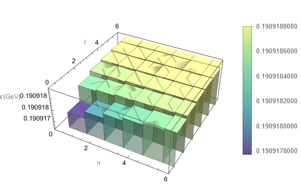
Figure 7: Graph of the energy spectrum in GeV, for $n$ ranging from $1$ to $6$ and $l$ ranging from $1$ to $6$. In natural units, $p_{z}=m=0.135$ GeV, $\eta=(4\pi)^{-1}0.303$.

Figure 8: Graph of the energy spectrum in GeV, for $n$ ranging from $1$ to $6$ and $l$ ranging from $1$ to $6$. In natural units, $p_{z}=0.135$ GeV, $m=1.34$ GeV, $\eta=(4\pi)^{-1}0.303$.

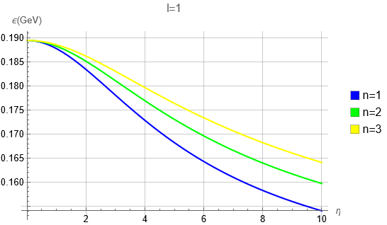
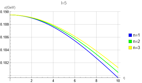
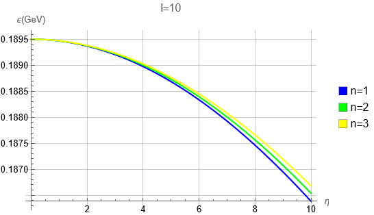
Figure 9: $\epsilon$ versus $\eta$ energy spectrum plot, for $n=1,2,3$, $l=1,5,10$. In natural units, $m=p_{z}=0.135$ GeV and $H_{0}=0.195\ \text{GeV}^{2}$.

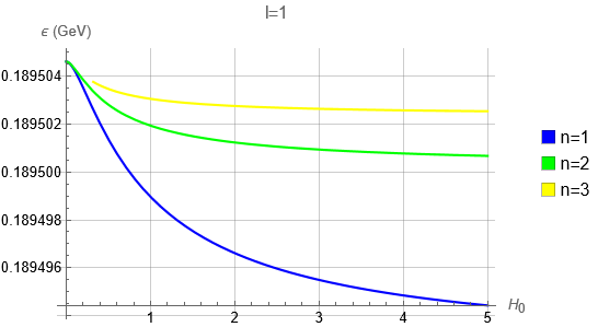
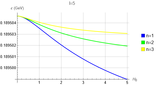
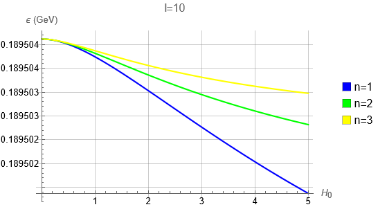
Figure 10: $\epsilon$ versus $H_{0}$ (in $\rm{GeV}^{2}$) energy spectrum plot, for $n=1,2,3$, $l=1,5,10$. In natural units, $m=p_{z}=0.134$ GeV and $\eta=\frac{0.303}{4\pi}$.

4 Conclusions

In this work we studied spin-0 bosons in a spacetime of a magnetic field with cosmological constant. The calculations have been made considering the metric proposed in [15]. We used $\pi^{0}$ as test particles and in order to have the possibility to achieve more significant effects, strong magnetic fields, of the order of the ones supposed to be produced in high energy heavy ion collisions. The Klein-Gordon equation for this spacetime has been determined and then solved. With these solutions it was possible to discuss the existence of the Landau levels, find numerical values and verify their dependence with the considered parameters. The influence of a scalar Coulomb-type potential has also been verified. As we can see in Fig. 10, the effect of the magnetic field $H_{0}$ has a very small influence on the energy levels, but small changes may be observed and increases with the value of the parameter $\eta$. The calculations presented are a result of a very specific kind of spacetime, but we may imagine that in a region near a source of a strong magnetic field, as a magnetar for example, a similar behaviour may occur and this kind of effect be observed in accurate experiments. This kind of observation is very important as far as it deals with the influence of the spacetime structure in quantum systems.

References

- [1] Leonard I Schiff “Possible new experimental test of general relativity theory” In Physical Review Letters 4.5 APS, 1960, pp. 215
- [2] Josef Lense and Hans Thirring “Über den Einfluss der Eigenrotation der Zentralkörper auf die Bewegung der Planeten und Monde nach der Einsteinschen Gravitationstheorie” In Physikalische Zeitschrift 19, 1918, pp. 156
- [3] B.. Abbot “Observation of Gravitational Waves from a Binary Black Hole Merger” In Physical Review Letters 116.6 American Physical Society (APS), 2016 DOI: 10.1103/physrevlett.116.061102
- [4] Albert Einstein “Lens-Like Action of a Star by the Deviation of Light in the Gravitational Field” In Science 84.2188, 1936, pp. 506–507 DOI: 10.1126/science.84.2188.506
- [5] S Refsdal and J Surdej “Gravitational lenses” In Reports on Progress in Physics 57.2, 1994, pp. 117
- [6] Christopher Thompson and Robert C. Duncan “The soft gamma repeaters as very strongly magnetized neutron stars - I. Radiative mechanism for outbursts” In Monthly Notices of the Royal Astronomical Society 275.2, 1995, pp. 255–300 DOI: 10.1093/mnras/275.2.255
- [7] C. Kouveliotou “An X-ray pulsar with a superstrong magnetic field in the soft gamma-ray repeater SGR 1806-20.” In Nature 393, 1998, pp. 235–237 DOI: 10.1038/30410
- [8] Umut Gürsoy, Dmitri Kharzeev and Krishna Rajagopal “Magnetohydrodynamics, charged currents, and directed flow in heavy ion collisions” In Phys. Rev. C 89 American Physical Society, 2014, pp. 054905 DOI: 10.1103/PhysRevC.89.054905
- [9] Adam Bzdak and Vladimir Skokov “Event-by-event fluctuations of magnetic and electric fields in heavy ion collisions” In Physics Letters B 710.1, 2012, pp. 171–174 DOI: https://doi.org/10.1016/j.physletb.2012.02.065
- [10] V. Voronyuk et al. “Electromagnetic field evolution in relativistic heavy-ion collisions” In Phys. Rev. C 83 American Physical Society, 2011, pp. 054911 DOI: 10.1103/PhysRevC.83.054911
- [11] Ts.I. Gutsunaev and V.S. Manko “On the gravitational field of a mass possessing a magnetic dipole moment” In Physics Letters A 123.5, 1987, pp. 215–216 DOI: https://doi.org/10.1016/0375-9601(87)90063-6
- [12] Ts.I. Gutsunaev and V.S. Manko “New static solutions of the Einstein-Maxwell equations” In Physics Letters A 132.2, 1988, pp. 85–87 DOI: https://doi.org/10.1016/0375-9601(88)90257-5
- [13] W B Bonnor “Static Magnetic Fields in General Relativity” In Proceedings of the Physical Society. Section A 67.3, 1954, pp. 225 DOI: 10.1088/0370-1298/67/3/305
- [14] M.A. Melvin “Pure magnetic and electric geons” In Physics Letters 8.1, 1964, pp. 65–68 DOI: https://doi.org/10.1016/0031-9163(64)90801-7
- [15] Martin Žofka “Bonnor-Melvin universe with a cosmological constant” In Physical Review D 99.4 APS, 2019, pp. 044058
- [16] Leonard Parker “One-Electron Atom in Curved Space-Time” In Phys. Rev. Lett. 44.23, 1980, pp. 1559 DOI: 10.1103/PhysRevLett.44.1559
- [17] Nicholas David Birrell, Nicholas David Birrell and PCW Davies “Quantum fields in curved space” Cambridge university press, 1984
- [18] Emilio Elizalde “Series solutions for the Klein-Gordon equation in Schwarzschild space-time” In Physical review D: Particles and fields 36, 1987, pp. 1269–1272 DOI: 10.1103/PhysRevD.36.1269
- [19] Subrahmanyan Chandrasekhar “The solution of Dirac’s equation in Kerr geometry” In Proceedings of the Royal Society of London. A. Mathematical and Physical Sciences 349.1659, 1976, pp. 571–575 DOI: 10.1098/rspa.1976.0090
- [20] L… Santos and C.. Barros Jr. “Scalar bosons under the influence of noninertial effects in the cosmic string spacetime” In Eur. Phys. J. C 77.3, 2017, pp. 186 DOI: 10.1140/epjc/s10052-017-4732-x
- [21] L… Santos and C.. Barros Jr. “Relativistic quantum motion of spin-0 particles under the influence of noninertial effects in the cosmic string spacetime” In Eur. Phys. J. C 78.1, 2018, pp. 13 DOI: 10.1140/epjc/s10052-017-5476-3
- [22] R… Vitória and K. Bakke “Rotating effects on the scalar field in the cosmic string spacetime, in the spacetime with space-like dislocation and in the spacetime with a spiral dislocation” In Eur. Phys. J. C 78.3, 2018, pp. 175 DOI: 10.1140/epjc/s10052-018-5658-7
- [23] Faizuddin Ahmed “Gravitational field effects produced by topologically nontrivial rotating space–time under magnetic and quantum flux fields on quantum oscillator” In Int. J. Mod. Phys. A 37.28n29, 2022, pp. 2250186 DOI: 10.1142/S0217751X2250186X
- [24] Faizuddin Ahmed “Klein–Gordon oscillator with magnetic and quantum flux fields in non-trivial topological space-time” In Commun. Theor. Phys. 75.2, 2023, pp. 025202 DOI: 10.1088/1572-9494/aca650
- [25] L… Santos, C.. Mota and C.. Barros Jr. “Klein–Gordon Oscillator in a Topologically Nontrivial Space-Time” In Adv. High Energy Phys. 2019, 2019, pp. 2729352 DOI: 10.1155/2019/2729352
- [26] Yi Yang et al. “The generalized Klein–Gordon oscillator with position-dependent mass in a particular Gödel-type space–time” In Int. J. Mod. Phys. A 36.03, 2021, pp. 2150023 DOI: 10.1142/S0217751X21500238
- [27] A.. Soares, R… Vitória and H. Aounallah “On the Klein–Gordon oscillator in topologically charged Ellis–Bronnikov-type wormhole spacetime” In Eur. Phys. J. Plus 136.9, 2021, pp. 966 DOI: 10.1140/epjp/s13360-021-01965-0
- [28] Tarek Imed Rouabhia, Abdelmalek Boumali and Hassan Hassanabadi “Effect of the Acceleration of the Rindler Spacetime on the Statistical Properties of the Klein–Gordon Oscillator in One Dimension” In Phys. Part. Nucl. Lett. 20.2, 2023, pp. 112–119 DOI: 10.1134/S154747712302019X
- [29] V.. Bezerra et al. “Casimir Effect in the Kerr Spacetime with Quintessence” In Mod. Phys. Lett. A 32.01, 2016, pp. 1750005 DOI: 10.1142/S0217732317500055
- [30] L… Santos and C.. Barros Jr. “Rotational effects on the Casimir energy in the space–time with one extra compactified dimension” In Int. J. Mod. Phys. A 33.20, 2018, pp. 1850122 DOI: 10.1142/S0217751X18501221
- [31] E.. Pinho and C.. Barros Jr. “Spin-0 bosons near rotating stars” In Eur. Phys. J. C 83.8, 2023, pp. 745 DOI: 10.1140/epjc/s10052-023-11907-y
- [32] Parisa Sedaghatnia, Hassan Hassanabadi and Faizuddin Ahmed “Dirac fermions in Som–Raychaudhuri space-time with scalar and vector potential and the energy momentum distributions” In Eur. Phys. J. C 79.6, 2019, pp. 541 DOI: 10.1140/epjc/s10052-019-7051-6
- [33] Abdullah Guvendi, Soroush Zare and Hassan Hassanabadi “Exact solution for a fermion–antifermion system with Cornell type nonminimal coupling in the topological defect-generated spacetime” In Phys. Dark Univ. 38, 2022, pp. 101133 DOI: 10.1016/j.dark.2022.101133
- [34] R… Vitória and K. Bakke “On the interaction of the scalar field with a Coulomb-type potential in a spacetime with a screw dislocation and the Aharonov-Bohm effect for bound states” In Eur. Phys. J. Plus 133.11, 2018, pp. 490 DOI: 10.1140/epjp/i2018-12310-9
- [35] L… Santos and C.. Barros Jr. “Dirac equation and the Melvin Metric” In Eur. Phys. J. C 76.10, 2016, pp. 560 DOI: 10.1140/epjc/s10052-016-4409-x
- [36] “NIST Handbook of Mathematical Functions Paperback and CD-ROM” Cambridge University Press, 2010, pp. 968
- [37] M.. Cunha, C.. Muniz, H.. Christiansen and V.. Bezerra “Relativistic Landau Levels in the Rotating Cosmic String Spacetime” In Eur. Phys. J. C 76.9, 2016, pp. 512 DOI: 10.1140/epjc/s10052-016-4357-5
- [38] G. De A Marques, Claudio Furtado, V.. Bezerra and Fernando Moraes “Landau levels in the presence of topological defects” In J. Phys. A 34, 2001, pp. 5945–5954 DOI: 10.1088/0305-4470/34/30/306
- [39] R.. Workman “Review of Particle Physics” In PTEP 2022, 2022, pp. 083C01 DOI: 10.1093/ptep/ptac097
- [40] K Bakke and C Furtado “On the Klein–Gordon oscillator subject to a Coulomb-type potential” In Annals of Physics 355 Elsevier, 2015, pp. 48–54