AirIMU: Learning Uncertainty Propagation for Inertial Odometry

Abstract

Accurate uncertainty estimation for inertial odometry is the foundation to achieve optimal fusion in multi-sensor systems, such as visual or LiDAR inertial odometry. Prior studies often simplify the assumptions regarding the uncertainty of inertial measurements, presuming fixed covariance parameters and empirical IMU sensor models. However, the inherent physical limitations and non-linear characteristics of sensors are difficult to capture. Moreover, uncertainty may fluctuate based on sensor rates and motion modalities, leading to variations across different IMUs. To address these challenges, we formulate a learning-based method that not only encapsulate the non-linearities inherent to IMUs but also ensure the accurate propagation of covariance in a data-driven manner. We extend the PyPose library to enable differentiable batched IMU integration with covariance propagation on manifolds, leading to significant runtime speedup. To demonstrate our method’s adaptability, we evaluate it on several benchmarks as well as a large-scale helicopter dataset spanning over 262 kilometers. The drift rate of the inertial odometry on these datasets is reduced by a factor of between 2.2 and 4 times. Our method lays the groundwork for advanced developments in inertial odometry. The source code is available at: https://github.com/haleqiu/AirIMU

I Introduction

Inertial Measurement Units (IMUs), capable of capturing three-axis angular velocity and acceleration, are an essential component in a wide range of intelligent devices. Due to their relative independence from external environmental factors, IMUs offer robust state estimation, especially in inertial-aided simultaneous localization and mapping (SLAM) systems paired with cameras [1], LiDAR [2], or multi-modal sensors [3]. Despite these advantages, the challenge of accumulated location drift persists due to sensing noise in IMUs [4]. Many SLAM algorithms address this issue by incorporating IMU measurements into pose graph optimization (PGO) with complementary sensors such as GPS to maintain scale consistency. Within the PGO framework, the incorporation of an appropriate IMU uncertainty model ensures the measurements’ reliability and optimizes the integration outcome. Therefore, accurate IMU integration and uncertainty modeling collectively play vital roles in inertial-aided SLAM algorithms.

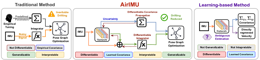
Figure 1: Left: Traditional methods with empirically-set uncertainty parameters often fail to capture noise accurately. Middle: AirIMU not only denoises the IMU data but also predicts the corresponding uncertainty of the integration. Notably, its covariance propagation is differentiable, promoting efficient training. Right: Learning-based algorithms can predict velocity and covariance, but their predictions lack interpretability and generality across different data domains.

Traditional inertial odometry algorithms offer versatile state estimation across various platforms, but face challenges in modeling the intricate and multifaceted noise inherent in the IMU. A notable advantage of these methods is that they offer high-frequency output with optimal guarantees for state estimations and control algorithms, ensuring compatibility with existing inertial navigation systems. Furthermore, these methods operate without assumptions on the data’s motion modality (e.g., pedestrian modality), making them generalizable. Their standard practice to mitigate the sensor noise involves using hand-crafted models with additive parameters, intrinsic matrices, and fixed uncertainty parameters [5, 6]. However, comprehensively modeling the complex and unpredictable noise of IMUs is infeasible using just manual calibration and empirical setups. The noise originates from multiple factors: extreme operational conditions, mechanical anomalies, electronic imperfections, and calculation ambiguities.

Learning-based inertial odometry employs neural networks to directly regress the velocity and its covariance [7, 8]. One notable limitation is their lack of interpretability. These methods implicitly replace the arithmetic functions of both IMU integration and covariance propagation with a neural network, which is subject to ambiguity. They often aren’t universally adaptable and tend to overfit to specific domains like pedestrian movement [9] or wheeled robots [10]. More importantly, they overlook covariance accumulation during IMU integration and fail to model the uncertainty inherent in pre-integration. These gaps hinder the incorporation of learning-based methods in multi-sensor fusion.

To optimize performance in multi-sensor fusion, we propose AirIMU, which serves the dual purposes of de-noising the IMU data and predicting the corresponding uncertainty of the pre-integration. Contrary to prior work that relied on basic IMU sensor models and fixed covariance assumptions, the AirIMU model learns the IMU sensors’ non-linearity and uncertainty in a data-driven manner. Given the challenges in labeling ground truth states and corresponding covariance, it’s impractical to label every IMU measurement. To address this, we’ve developed a differentiable batched IMU integrator and a covariance propagator on manifolds. This allows us to supervise both the IMU sensor model and the uncertainty model even with limited labels. Grounded on PyPose[11], our model facilitates matrix operations in covariance propagation, utilizing cumulative product techniques to enhance training speed. Instead of learning an inertial model directly, we utilize a robust kinematic model to ensure adaptability across various platforms. Furthermore, our model can adjust to different sensor frequencies and provide an accurate covariance, boosting its multi-sensor fusion capabilities. Our model can seamlessly integrate with a wide range of existing inertial aided state estimation algorithm. This paper is the first to employ differentiable covariance propagation for a deep model of IMU integration’s uncertainty.

In summary, the main contributions of this paper are:

• Empower AirIMU model to learn the IMU uncertainty through differentiable integration and covariance propagation grounded on PyPose library. Additionally, we illustrate the effectiveness of the learned uncertainty in a GPS-IMU PGO experiment.

• Propose an uncertainty-aware IMU odometry algorithm, which is compatible with a variety of platforms. We demonstrate its superior performance in short-term integration in public datasets: EuRoC [12] and TUM-VI [13]. We further evaluate AirIMU on a large-scale Visual Terrain Navigation dataset spanning over 262 $\mathrm{km}\text{/}$.

• Employ batched operations and the cumulative product in our tool package, which accelerate the training process. This package is now open-source at: https://pypose.org/tutorials/imu

II Related Works

II-A IMU Calibration

Meticulous calibration of the IMU is indispensable. Such calibration can either be facilitated through self-measurements under static conditions [5] or with the aid of external devices, such as shakers and rate tables. Kalibr [14] is one of the most widely used calibration algorithm, which determines the extrinsic parameters between the camera and IMU, as well as the IMU intrinsic parameters. Within these IMU sensor models, a constant additive offset is commonly incorporated to provide an approximation of the sensor’s bias. To enhance the precision of the IMU sensor model, especially for low-cost Micro-Electro-Mechanical Systems (MEMS) IMUs, factors like orthogonal error, acceleration sensitivity, thermal effects [15], and even Coriolis force [16] are rigorously addressed.

As discussed in the Introduction section (Section I), accurately modeling the IMU sensor with a straightforward arithmetic model is challenging due to the intricacies of the sensor’s physical condition and its operation environment. Inspired by the advancements in deep learning, some researchers explore data-driven model to implicitly calibrate and denoise the IMU observations [17, 18, 19]. Nonre et al [17] leverage deep reinforcement learning for IMU calibration. Brossard et al [18] train a Convolutional Neural Network (CNN) to denoise the low-frequency error in gyroscopes integration. Zhang et al. [19] employed Long Short-Term Memory (LSTM) network for preprocessing raw IMU. These processed IMU observations are subsequently channeled into a filter-based visual-inertial odometry system. Deep IMU Bias [20], utilizes neural networks to model the sensor bias, and incorporates the learned bias as an additional observation during graph optimization. These researches showcase the potential of data-driven methods to enhance IMU calibration. This, in turn, improve the performance of the inertial-aided algorithms, especially when assessing the IMU’s physical conditions becomes challenging.

It is worth noting that despite the advancements made in data-driven IMU calibration methods, none of the referenced algorithms have explicitly tackled the challenge of modeling the uncertainty for IMU integration. These methods [19, 20] use constant empirical covariance parameters during the graph optimization. However, as the IMU sensor model undergoes optimization through these data-driven algorithms, there arises a potential issue: the original covariance model may no longer align accurately with the updated sensor model, which can subsequently lead to inaccuracies in the inertial navigation.

II-B IMU uncertainty model

Traditional methods propagate the IMU’s uncertainty using the IMU kinematics model [4]. This strategy is widely used in the IMU dead-reckoning algorithms and multi-modal SLAM, e.g., VinsMono [1]. One limitation is that it requires manual calibration of the uncertainty parameters. A commonly used solution for this is the Allen variance[21], which helps identifying and quantifying the noise throughout the integration process. Another strategy is to model the uncertainty with a data-driven model. The AI-IMU [10] proposes a dead-reckoning EKF algorithm for the wheeled vehicles, which assumes that the lateral velocity and vertical velocity are approximately null. To model the confidence degree of this null assumptions, the author train a CNN network from IMU to predict two constant uncertainty parameters that corresponding to lateral velocity and vertical velocity. In TLIO [7], the author jointly train a uncertainty model that estimate the covariance of the estimated translation in a fixed temporal window. For the state transition where the IMU integration happened, TLIO also use a constant empirical covariance parameter.

II-C Learning-based Inertial Odometry

A growing trend of leveraging a machine learning model on inertial navigation has been witnessed, such as IMU odometry network [22, 23], EKF-fused IMU odometry [7, 8, 24]. In RIDI [22], a supervised Support Vector Machine (SVM) classifier is introduced to determine IMU placement modes (e.g., handheld, bag) using accelerometer and gyroscope measurements. Mode-specific Support Vector Regressors (SVRs) are then employed to estimate pedestrian velocities based on motion types, enabling corrective adjustments to sensor readings. IONet [23] introduced deep learning to regress agent velocity within a fixed temporal window, subsequently integrating agent poses using the regressed speeds. Building on this concept, RoNIN [9] explores diverse neural network architectures including Temporal Convolutional Networks (TCN), Long Short-Term Memory (LSTM), and ResNet. RIO [24] explores rotation-equivalence as a self-supervisory mechanism for training inertial odometry models. These studies utilize data-driven velocity estimation models to replace the velocity integration process, thereby alleviating the drift issues associated with IMU double integration. Such strategy is equivalent to training a network to fit the well-defined IMU kinematics function, as a result of which, it lacks accuracy guarantee in relative pose estimation compared to IMU integration. Inspired by these IMU odometry network studies, TLIO [7] integrates the data-driven velocity estimation model with the IMU kinematics model through a stochastic-cloning Extended Kalman Filter (EKF). This integrated approach jointly estimates position, orientation, and sensor biases using solely pedestrian IMU data. IDOL [8] further extends this framework with a data-driven orientation estimator, generating more accurate results with better continuities.

Although these strategies succeed in pedestrian datasets like RoNIN [9], wheeled odometry datasets like KITTI, they share certain limitations: (i) The learned velocity model lacks an optimal guarantee due to the inherent ambiguity involved in fitting the integration function. (ii) The velocity estimation heavily relies on the human prior learned by the neural network. This reliance, such as the alignment of velocity’s direction with acceleration’s direction, becomes impractical across different data domain. (iii) Many of these researches were developed based on strong assumptions, which were infeasible in real applications. For example, they either assuming that the model’s input is in the ground-truth coordinate frame with a fixed temporal window or the ambiguity of the pitch and roll can be eliminated by aligning the y-axis with gravity.

III AirIMU Model

III-A Problem Preliminary

In this work, we assume a body frame $\{B\}$ with the IMU sensor signal and a world frame $\{W\}$ with the ground truth. Many existing learning-based inertial algorithms presume that ground truth orientations are available to transform the raw input from the body frame $\{B\}$ to world frame $\{W\}$ or a Heading-Agnostic Coordinate Frame (HACF) defined in [9]. However, the ground truth orientation may not be available in the real applications. We aim to predict the state of the robot $x$, including orientation $R$, velocity $v$, and position $p$ with respect to the world frame $\{W\}$, which is defined as:

$${}^{W}x_{i}\triangleq[{}^{W}{R}_{i},{}^{W}v_{i},{}^{W}p_{i}]\in\text{SO3}\times\mathbb{R}^{6},$$ (1)

The raw IMU sensor includes the 3-axis acceleration $a$ and 3-axis angular velocity $w$ from the body frame $\{B\}$:

$${}^{B}w_{i}\in\mathbb{R}^{3},\ {}^{B}a_{i}\in\mathbb{R}^{3}.$$ (2)

The formulation of IMU pre-integration is well-developed in [4]. The integration of the IMU from $i$-th frame to $j$-th frame follows Newton’s kinematic laws.

$$\begin{split}{\Delta}R_{ij}&=\int_{t\in[t_{i},t_{j}]}{}^{B}w_{k}\ dt\\ {\Delta}v_{ij}&=\int_{t\in[t_{i},t_{j}]}R_{k}{}^{B}a_{k}\ dt\\ {\Delta}p_{ij}&=\int\int_{t\in[t_{i},t_{j}]}R_{k}{}^{B}a_{k}\ dt^{2}\ ,\end{split}$$ (3)

where the raw IMU measurements of accelerator ${}^{B}a_{k}$ and gyroscope ${}^{B}w_{k}$ are from the $k$-th frame with the body coordinate $\{B\}$. Given the increments from frame $i$ to frame $j$ on the rotation ${\Delta}R_{ij}$, velocity ${\Delta}v_{ij}$ and position ${\Delta}p_{ij}$, the $j$-th state of the robot ${}^{W}x_{j}$ can be predicted through:

$$\begin{split}\tensor[^{W}]{R}{{}_{j}}&={\Delta}R_{ij}\otimes{}^{W}R_{i}\\ {}^{W}v_{j}&={}^{W}R_{i}*{\Delta}v_{ij}+{}^{W}v_{i}\\ {}^{W}p_{j}&={}^{W}R_{i}*{\Delta}p_{ij}+{}^{W}p_{i}+{}^{W}v_{i}\Delta t_{ij},\end{split}$$ (4)

where the ${}^{W}R_{i}$, ${}^{W}v_{i}$ and ${}^{W}p_{i}$ is the initial state of the integration in the world coordinate $\{W\}$. We assume the noise model of the gyroscope and accelerometer as a zero-mean Gaussian noise term $\eta^{gyro}_{k}$ and $\eta^{acc}_{k}$ for frame k. The noise of the integrated states can be characterized as:

$$[\delta\phi_{ij}^{T},\delta v_{ij}^{T},\delta p_{ij}^{T}]^{T}\sim\mathbb{N}(0_{9\times 1},\Sigma_{ij}),$$ (5)

where $\Sigma_{ij}$ is the covariance matrix propagated from $\eta^{gyro}_{k}$ and $\eta^{acc}_{k}$. We will show more details of the covariance propagation in the following sections. To render the model operable in realistic scenarios, the AirIMU model train and predict the learned corrected acceleration and angular velocity ${}^{B}\tilde{a},{}^{B}\tilde{w}$ and the corresponding uncertainty $\eta^{gyro},\eta^{acc}$ from the IMU body frame $\{B\}$. We utilize the IMU kinematic model 4 to estimate the states ${}^{W}x_{j}$, and more importantly, to propagate the corresponding covariance matrix $\Sigma_{i,j}$.

III-B Efficient De-noising and Uncertainty Module

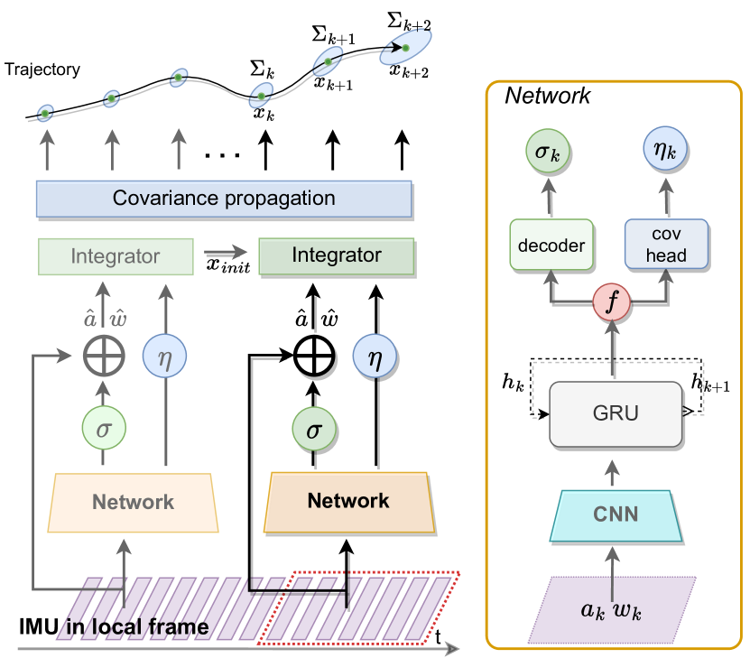
Figure 2: Right: We employ CNN-GRU encoder to capture IMU features ($f$) from raw IMU accelerometer ($a_{k}$) and gyroscope ($w_{k}$). Subsequently, these features are decoded to obtain IMU corrections ($\sigma_{acc}$, $\sigma_{gyro}$). Left: We add the raw data with corrections, generating corrected IMU measurements ($\hat{a}_{k}$ and $\hat{w}_{k}$). The learned uncertainties ($\eta$) are propagated to estimate the corresponding covariance matrix ($\Sigma$).

To supervise the learnable modules within the IMU body frame $\{B\}$, we’ve built a differentiable integrator and covariance propagator. This construction ensures efficient back-propagation of gradients from the world frame $\{W\}$ states to the IMU body frame $\{B\}$. For this process, we employ batched operations and the cumulative product to acclerate IMU integration. Additionally, we’ve reformulated the covariance propagation to hasten the estimation of covariance.

As shown in Figure 2, the system comprises an encoder and decoder structure, where the encoder consists of convolutional neural network and Gated Recurrent Unit (GRU) layers, responsible for processing the raw input acceleration $a$ and angular velocity $w$. The de-noise model $f_{\pi}$ takes a temporal input of the IMU data and predicts the corrections $\sigma^{gyro},\sigma^{acc}$ in the body frame $\{B\}$, as shown in the following:

$$[\sigma^{gyro},\sigma^{acc}]=f_{\pi}(w,a),$$ (6)

where $\pi$ represents the learnable parameters of the de-noising network. The IMU corrections are then added to the original signal to generate the corrected acceleration and angular velocity $\tilde{a}$ and $\tilde{w}$, as depicted by:

$$\tilde{a}=a+\sigma_{acc},\ \tilde{w}=w+\sigma_{gyro}$$ (7)

With the shared encoder features, we employ another head to predict the uncertainty of each corresponding frame. This uncertainty is predicted by a covariance model denoted as $\Sigma_{\theta}(w,a)$, yielding the following equation:

$$[\eta^{gyro}_{k},\eta^{acc}_{k}]=\Sigma_{\theta}(w,a)$$ (8)

Where $\theta$ represents the learnable parameters of the covariance model, which predict the uncertainty of the IMU pre-integration in each frame $k$.

The propagation of the IMU covariance is also following the kinematic model of the robot. We apply a similar uncertainty propagation strategy as [4] to model the covariance matrix $\Sigma_{ij}$ of the IMU integration from frame i to frame i+1 through iterative propagation:

$$\Sigma_{i,i+1}=A\Sigma_{i,i}A^{T}+B_{g}\mathrm{diag}(\eta^{gyro}_{i})B_{g}^{T}+B_{a}\mathrm{diag}(\eta^{acc}_{i})B_{a}^{T}$$ (9)

where state transition matrix A is defined as

$$A=\begin{bmatrix}{\Delta}R_{ik+1}^{T}&0_{3*3}&0_{3*3}\\ -{\Delta}R_{ik}(a_{k}^{\wedge}){\Delta}t&I_{3*3}&0_{3*3}\\ -1/2{\Delta}R_{ik}(a_{k}^{\wedge}){\Delta}t^{2}&I_{3*3}{\Delta}t&I_{3*3}\end{bmatrix}$$ (10)

and the B matrix takes the frame-by-frame uncertainty of the acceleration and the angular velocity.

$$B_{g}=\begin{bmatrix}J_{r}^{k}\Delta t\\ 0_{3*3}\\ 0_{3*3}\end{bmatrix},\ \ \ B_{a}=\begin{bmatrix}0_{3*3}\\ {\Delta}R_{ik}{\Delta}t\\ 1/2{\Delta}R_{ik}{\Delta}t^{2}\end{bmatrix},$$ (11)

However, during the training, the requirement to propagate covariance across numerous extended sequences, given batched inputs, makes it impractical to compute the covariance matrix in an iterative manner as equation 9. So, we reformulate the propagation process into a summation over two list of the matrix products $C^{A}$ and $C^{B}$:

$$\begin{split}C^{A}_{i,j}=&[\prod_{k=j}^{i}A_{k},\prod_{k=j}^{i+1}A_{k},...,A_{j},I_{9\times 9}]\\ C^{B}_{i,j}=&[\Sigma_{i,i},B_{i},...,B_{j-1},B_{j}],\\ \end{split}$$ (12)

We calculate the integration covariance matrix $\Sigma_{i,j+1}$ from:

$$\Sigma_{i,j+1}=\sum_{i}^{j}C^{A}C^{B}{C^{A}}^{T}$$ (13)

The benefits of this formulation are that we can first use cumprod and cumsum to accelerate the calculation of $C$ and $D$ from frame i to j, which reduce the time complexity from $O(N)$ to $O(\log N)$. Second, we fully utilize the computation power of PyTorch and PyPose with batched operations, which can accelerate the training provess through a long sequence.

III-C Loss Function and Supervision

To supervise the AirIMU model, the most straight-forward way is to obtain the truth corrected IMU measurements alongside corresponding uncertainty. This is impracticable in real-world applications. To supervise the model, we design the loss function on position, orientation, and translation in the world frame $\{W\}$.

$$\begin{split}L_{r}&=\|\log(R_{i}\otimes\hat{R}_{i})\|_{h}\\ L_{v}&=\|v_{i}-\hat{v}_{i}\|_{h}\\ L_{p}&=\|p_{i}-\hat{p}_{i}\|_{h}\\ \end{split}$$ (14)

where the $\|\cdot\|_{h}$ denotes the Huber function. To supervise the rotation in manifold, we transform the orientation error to $\log$ space in the loss function (14). This can help the learnable module to capture the noise in orientation.

To constrain the covariance, we use a similar loss function form that derived in [25]

$$L=\frac{(y-f(w,a))^{2}}{2\Sigma_{\theta}(w,a)}+\frac{1}{2}\ln|\Sigma_{\theta}(w,a)|$$ (15)

where $y$ is the ground truth and $f(w,a)$ output the integrated state. The $\Sigma_{\theta}(x)$ denotes covariance model that predicts the covariance matrix given the learned uncertainty $\eta$.

IV System & Implementation

As we have discussed in the previous sections, IMU pre-integration introduces inevitable drift in the pose estimation. To recover such drift, We introduce the other sensors (i.e., GPS) to fuse with the IMU pre-integration. As shown in Fig. 3, we show an example PGO with the AirIMU model and GPS signal, in which we showcase an example of how the learned covariance can benefit the optimization.

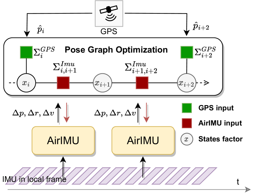
Figure 3: Pose graph optimization of a GPS signal with the IMU pre-integration. The state of the graph is defined as $x_{i}$ constrained by two different observations: IMU ($\Delta p$, $\Delta v$ and $\Delta r$) and GPS ($\hat{p}_{i}$). The gradient can be back-propagated through the IMU pre-integration and the covariance propagation.

We show a graph optimization example with a factor of GPS. In the pose graph optimization, the residual of the IMU measurement is defined as:

$$e^{IMU}_{ij}(\Delta v_{ij},\Delta p_{ij},\Delta r_{ij},)=\begin{bmatrix}{\Delta}R_{ij}\otimes{}^{W}R_{i}\otimes({}^{W}R_{j})^{-}1\\ {}^{W}v_{i}+{}^{W}R_{i}*{\Delta}v_{ij}-{}^{W}v_{j}\\ {}^{W}p_{i}+{}^{W}R_{i}*{\Delta}p_{ij}-{}^{W}p_{j}\end{bmatrix},$$ (16)

The corresponding covariance matrix of the IMU integration is defined in 9 as $\Sigma^{IMU}_{ij}$. We define the GPS signal and provide the measurements $\hat{p}_{i}\in R^{3}$ which constrains the position of the state. We design the residual of GPS measurements as:

$$e^{GPS}_{i}(\hat{p}_{i})=\hat{p}_{i}-p_{i}$$ (17)

where the measurement of the GPS is $\hat{p}_{i}$ with a corresponding covariance matrix which is defined to be a diagonal matrix $\Sigma^{GPS}_{i}$. The pose graph optimization with the residual of both the $e^{GPS}_{i}(\hat{p}_{i})$ and GPS can be:

$$X^{*}=\operatornamewithlimits{argmin}_{X}\{\sum_{k\in G}\|e^{GPS}_{k}\|^{2}_{\Sigma^{GPS}_{k}}+\sum_{l\in L}\|e^{IMU}\|^{2}_{\Sigma^{IMU}_{l}}\}$$ (18)

where $G$ and $L$ is the set of GPS and IMU observations. It can be solved by Levenberg-Marquardt algorithms.

V Experiments

In our experiment, we assess the precision of our IMU model, with a particular emphasis on the potency of the learned uncertainty model within the back-end PGO of multi-sensor fusion system. From Section V-A to Section V-B, we demonstrate the superior performance of our method in IMU pre-integration compared to existing IMU de-noise algorithms and learning inertial odometry. In Section V-C, our ablation study of the learned uncertainty model within a GPS-PGO experiment reveals an average improvement by 30% when utilizing the learned covariance. Section V-D demonstrates the potential of the AirIMU model in GPS-denied helicopter navigation using a high-end IMUs. This assessment spans cruising distance over 262 [km], providing a realistic and challenging environment for evaluating our method.

In order to establish a Baseline for comparison, we implement the IMU integration using PyPose [11] based on the work of Foster et al. [4]. The Baseline IMU integration serves as a reference for evaluating the performance of the AirIMU model in the context of IMU integration.

Each dataset contains IMU with diverse mechanical conditions and modalities, and considering that every sensor comes with its distinct noise model, training a universal model that can generalize across varied IMUs without compromising accuracy is infeasible. Therefore, we opt to train distinct sensor models tailored to different IMU types.

V-A IMU Pre-integration Accuracy

In this section, we demonstrate the effectiveness of the AirIMU model for IMU pre-integration by comparing it against two existing learning-based IMU denoising methods: Zhang et al. [19] and Brossard et al. [18], utilizing the EuRoC dataset [12]. Additionally, we showcase how our method enhances the integration precision of the traditional calibration algorithm, Kalibr [14], when tested on the TUM-VI dataset [13].

Learning-based IMU denoising: In this analysis, we compare the pre-integration performance of the AirIMU model with other learning-based de-noising methods. Our objective is to assess the AirIMU model’s effectiveness in enhancing IMU measurements quality and its influence on subsequent visual-inertial fusion systems.

Both Zhang et al. and Brossard et al were evaluated using different visual-inertial odometry and different evaluation benchmarks. As a result, direct comparison of absolute positional error is difficult to assess the effectiveness of the IMU denoising module. Specifically, Zhang et al. proposed a denoising approach that utilizes a bi-directional LSTM network, where preprocessed IMU measurements are then passed to their own visual-inertial baseline for further analysis. On the other hand, Brossard et al. applied CNN architecture to denoise the gyroscope measurements, which are subsequently used as input to the Open-Vins framework [26] for visual-inertial fusion. Considering these differences, in our evaluation, we compare each method separately using the benchmarks proposed in their papers respectively.

For the EuRoC dataset, we split the training set and the testing set using the same setting as Zhang et al. and Brossard et al. Zhang et al. reported the results of positional RMSE (P-RMSE) and rotational RMSE (R-RMSE) over ten frames of IMU measurements on the EuRoC dataset. Thus, we also evaluate 10-frame IMU pre-integration results in Table I. Notably, our method achieves an accuracy ten times superior to their reported P-RMSE and R-RMSE for short-term integration.

TABLE I: IMU integration result of 10 frames on EuRoC Dataset with P-RMSE (Unit: $\mathrm{cm}\text{/}$) and R-RMSE (Unit: $\mathrm{\SIUnitSymbolDegree}\text{/}$)

Seq.	Zhang et al. [19]		Baseline		AirIMU
	rot	pos	rot	pos	rot	pos
MH02	0.250	0.280	0.401	0.034	0.022	0.024
MH04	0.370	0.580	0.400	0.053	0.025	0.045
V103	0.670	0.530	0.402	0.044	0.033	0.036
V202	0.680	0.830	0.418	0.026	0.031	0.025
V101	1.620	0.300	0.398	0.028	0.023	0.018

Moreover, Zhang et al. provided P-RMSE values over specific time intervals: 0.5, 1, 2, and 3 seconds. Their reported values were approximately 0.05, 0.10, 0.40, and 0.75 meters, respectively. In contrast, using the same intervals, our method achieved P-RMSE values of 0.011, 0.038, 0.127, and 0.27 meters. This translates to an average improvement of three times in terms of positional accuracy. Additionally, we present the velocity RMSE results in Fig. 4.

Brossard et al. reported their findings using the Absolute Orientation Error (AOE). Given the nature of noise accumulation over time in IMU integration, we argue that gauging relative orientation with R-RMSE offers a more consistent metric on short-term integration. Consequently, our evaluation includes both AOE and the R-RMSE over a 1 $\mathrm{s}$ interval. To ensure a fairness and clarity, we re-trained the Gyro de-noising network released by Brossard et al.

TABLE II: Gyroscope integration on EuRoC Dataset, we show the AOE and the ROE (Unit: $\mathrm{\SIUnitSymbolDegree}\text{/}$).

Seq.	Brossard et al. [18]		Baseline		AirIMU
	AOE	R-RMSE	AOE	R-RMSE	AOE	R-RMSE
MH02	9.95	0.15	123.03	4.30	1.15	0.06
MH04	5.49	0.13	130.62	4.52	1.34	0.08
V103	2.65	0.18	119.78	4.48	1.92	0.21
V202	4.83	0.30	116.90	4.69	6.21	0.37
V101	3.94	0.39	114.24	4.52	2.19	0.14
Avg.	5.37	0.23	120.91	4.50	2.56	0.17

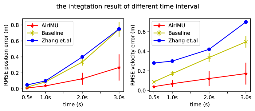
Figure 4: We present the RMSE error of both translation and velocity over intervals of 0.5$\mathrm{s}$, 1$\mathrm{s}$, 2$\mathrm{s}$, and 3$\mathrm{s}$. The results illustrate the accumulation of error throughout the integration, where the AirIMU exhibiting a reduced error after integration.

The EuRoC dataset contains a significant gyroscope offset, leading to drift in the orientation. As shown in Table. II, our model consistently outperformed other methods, showing superior accuracy and reliability across both the entire trajectory and local segments.

TABLE III: Ablation study of the GPS PGO with 1 Hz on the EuRoC dataset with different covariance settings.

Seq.	MH02	MH04	V103	V202	V101
AirIMU w/ learned Cov	0.1026 $\pm$ 0.0035	0.1024 $\pm$ 0.0039	0.1039 $\pm$ 0.0028	0.1060 $\pm$ 0.0046	0.1019 $\pm$ 0.0041
Raw IMU w/ learned Cov	0.1184 $\pm$ 0.0041	0.1327 $\pm$ 0.0048	0.1310 $\pm$ 0.0051	0.1569 $\pm$ 0.0078	0.1265 $\pm$ 0.0055
AirIMU w/ VinsMono Cov	0.1484 $\pm$ 0.0044	0.1486 $\pm$ 0.0049	0.1547 $\pm$ 0.0057	0.1540 $\pm$ 0.0049	0.1469 $\pm$ 0.0039
Raw IMU w/ VinsMono Cov	0.1493 $\pm$ 0.0044	0.1491 $\pm$ 0.0050	0.1549 $\pm$ 0.0058	0.1542 $\pm$ 0.0051	0.1478 $\pm$ 0.0041
Results show the mean and the standard deviation with ATE in meter $\mathrm{m}\text{/}$.

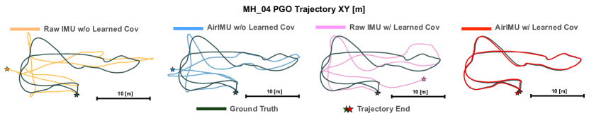
Figure 5: Qualitative analysis of the IMU-centric GPS PGO results. In this experiment, the GPS frequency is set to 0.1 Hz. Despite using identical IMU measurements, AirIMU with a learned covariance yields the optimal fusion results.

Traditional Calibration Algorithms: As described in II-A, traditional methods typically employ statistical strategies to calibrate IMU bias. For the TUM-VI dataset [13], raw data was calibrated using Kalibr [14]. This context allows us to examine whether our AirIMU model can further improve the traditional IMU calibration methods.

For our experiments on the TUM-VI dataset, we selected sequences from room 1, room 3, and room 5 for training, while using the remaining sequences for evaluation. It’s important to note that this dataset provides ground truth poses only in specific segments within the Vicon room. Therefore, we conducted integration through the entire sequences focusing our comparison on segments with available ground truth data. We compare the AOE and P-RMSE across the entire trajectory.

As shown in Table. IV, traditional calibration algorithms like Kalibr have effectively corrected offsets in the gyroscope data, leading to precise orientation estimations. Both AirIMU and Baseline method achieve high accuracy in rotation, registering 2.17^∘ and 1.49^∘ respectively. However, in terms of translation, significant drift occurs due to accelerometer noise, resulting in an average ATE of 73.53 $\mathrm{m}\text{/}$. In comparison, the AirIMU model substantially reduces this drift caused by IMU noise, achieving positional accuracy of 54.61 $\mathrm{m}\text{/}$.

TABLE IV: Pre-integration over entire trajectories of TUMVI dataset. We show AOE (Unit: $\mathrm{\SIUnitSymbolDegree}\text{/}$) and P-RMSE (Unit: meter).

Seq.	Baseline + Kalibr [14]		AirIMU
	AOE	P-RMSE	AOE	P-RMSE
room2	3.02	111.21	1.17	78.93
room4	1.69	75.60	1.30	55.82
room6	1.81	33.77	2.02	29.08
Avg.	2.17	73.53	1.49	54.61

V-B Learning-based inertial odometry

In Section II-C, we identified two main approaches to learning-based inertial odometry. The first utilizes end-to-end trained networks to estimate velocity. Within this category, we examined the estimation results derived from a ResNet, a model prevalently employed in methods such as TLIO [7] and RONIN [9]. Following the training script from TLIO, we used a 1D ResNet as the primary architecture to predict velocity.

The second approach involves EKF-fused inertial odometry, where outputs from neural networks are combined with an Extended Kalman Filter (EKF). When integrating the neural network’s predictions with raw IMU signals, the EKF in TLIO adeptly addresses system biases, thereby enhancing the accuracy of odometry estimations. For this category, we referenced results provided by [19].

We assessed the P-RMSE over an interval of 200 frames (equivalent to 1s), comparing these values to the short-term integration outcomes from AirIMU and Baseline in Table. V. When compared to the output from the directly regressed neural network, the pre-integration results from the AirIMU demonstrate a substantially greater accuracy — by a factor of 17. This distinction is especially noticeable when we consider the drone data. Unlike the pedestrian dataset, which might possess clear motion patterns or modalities, the dynamics of the drone data remain unpredictable, making it challenging for the neural network to accurately predict the velocity.

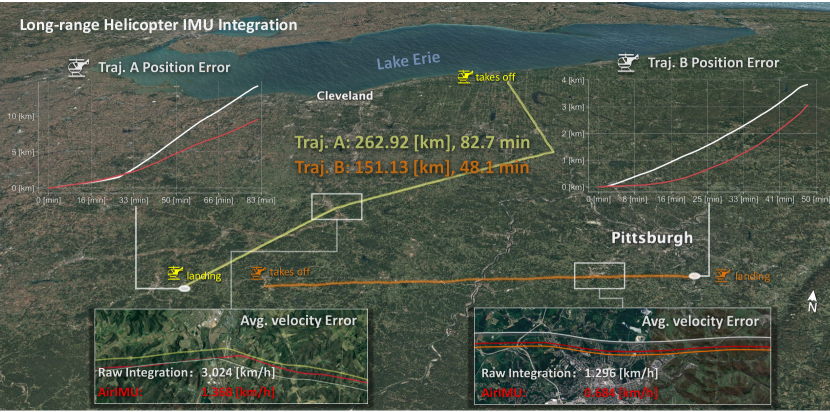
Figure 6: Trajectories of Visual Terrain Navigation Dataset. We show the positional error and the speed error of the raw IMU pre-integration and the AirIMU model.

TABLE V: The P-RMSE of IMU integration over 1 second (200 frames) on EuRoC dataset (Unit: meter).

Seq.	Baseline	ResNet	TLIO	AirIMU
MH02	0.0835	0.4858	0.3030	0.0194
MH04	0.0831	0.9068	0.8230	0.0286
V103	0.1087	0.6417	0.6530	0.0424
V202	0.0718	0.6864	0.5090	0.0684
V101	0.2788	0.5176	0.3430	0.0299

V-C IMU-centric graph optimization

The covariance model of the IMU pre-integration is pivotal when fusing the IMU with other sensors, such as the GPS and camera. To assess the effectiveness of our learned uncertainty proposed in the AirIMU model, we conducted an ablation study using PGO on EuRoC dataset. The specifics of this implementation can be found in Fig. 3.

A comprehensive evaluation of the IMU covariance requires controlling the noise from the fused sensors. To this end, we generate simulated GPS signals with a Gaussian noise of 0.1 $\mathrm{m}\text{/}$ at a frequency of 1 Hz. The PGO experiment is performed with following settings:

1. AirIMU with proposed learning covariance model.

2. Raw IMU with learned covariance model from (a).

3. AirIMU with the covariance parameters from the VinsMono’s setting [1].

4. Raw IMU with the covariance matrix from VinsMono’s setting (same as c).

The proposed covariance matrix of (a) is propagated through the Equation. 9 with the learned uncertainty model in $\Sigma_{\theta}(w,a)$. The covariance matrix of (b) is calculated by the VinsMono’s EuRoc configuration, where the noise standard deviation of accelerometer $\eta^{\text{acc}}=0.08$ and the noise standard deviation of gyroscope $\eta^{\text{gyro}}=0.004$. To ensure a fair comparison, we repeated the experiment 10 times with different GPS signals and random seeds. We summarize the mean Absolute Translation Error (ATE) and the standard deviation in Table. III. The application of the AirIMU model with its learned covariance significantly enhanced the PGO results. Compared to the results with the VinsMono’s covariance (c), the PGO with the learned covariance model improve 31.58$\%$, reducing the ATE from 0.1505 to 0.1033.

To delve deeper into the significance of the learned covariance, we conducted a qualitative analysis of the PGO experiments with a lower GPS frequency, where GPS signals are only observed every 10 seconds. As shown in Fig. 5, the precision of the IMU measurements and the associated covariance model plays a decisive role in the PGO results.

V-D Large-scale Helicopter Integration

Many existing methods have been evaluated in indoor environments or on small-scale datasets defined by limited duration and slower speeds. To bridge this gap, we employed Visual Terrain Relative Navigation dataset from a Bell 206L (Long-Ranger) helicopter. As shown in Fig. 6, this dataset encompasses flights over 262 km, featuring average speeds over 150 $\mathrm{km}\text{/}\mathrm{h}$ and cruising heights between 200 and 500 meters. This presents a robust testing ground for the AirIMU model’s capabilities.

For model training, we selected a segment from Flight B as the training data, using the remaining data for performance evaluation. Each flight in this dataset has a duration exceeding 40 minutes. Given the large cruising time, we sought to expedite training and enhance robustness by removing the GRU layer from our feature encoder. Owing to the high-end IMU sensor (NG LCI-1), only minimal drift is observed. We utilized the AirIMU to integrate the entire trajectory, assessing integration quality via speed error. Additionally, landing drift was also measured by comparing the integrated trajectory’s endpoint with the actual landing spot.

As shown in Table Fig. 6, compared to the Baseline method, the AirIMU model demonstrates remarkable enhancements. For Flight A, there’s a speed error reduction of 42.8% (from 3.02 $\mathrm{km}\text{/}\mathrm{h}$ to 1.37 $\mathrm{km}\text{/}\mathrm{h}$). Flight B experiences a reduction of 50% (from 1.29 $\mathrm{km}\text{/}\mathrm{h}$ to 0.68 $\mathrm{km}\text{/}\mathrm{h}$), proving the AirIMU model’s efficiency in estimating helicopter velocities. Regarding the landing drift, the AirIMU model significantly curtails discrepancies. For Flight A, the drift reduces from 3968 $\mathrm{m}\text{/}$ to just 1064 $\mathrm{m}\text{/}$. Flight B sees a reduction from 1228 $\mathrm{m}\text{/}$ to 479 $\mathrm{m}\text{/}$. This experiment showcase the generalizability of the AirIMU in the large-scale inertial navigation tasks.

VI Conclusion and Discussion

We propose an uncertainty-aware inertial odometry that empowers the system to learn the IMU uncertainty model via the differentiable covariance propagation. To demonstrate the efficacy of the learned covariance model, we conducted an ablation study on a GPS PGO experiment, reveling that the learned covariance improved 31% of the PGO results. Our experiments demonstrate that our AirIMU model is not only excel at the regular indoor environments with straightforward motion modality, but also perform well with a large-scale helicopter dataset over 262 $\mathrm{k}\mathrm{m}$. Additionally, we open-source the differentiable IMU integrator and the covariance propagation which is implemented in the PyPose framework. Given these advancements, we remain optimistic that the proposed method can provide a strong foundation for further research in inertial-aided state estimation and multi-sensor fusion.

References

- [1] T. Qin, P. Li, and S. Shen, “Vins-mono: A robust and versatile monocular visual-inertial state estimator,” IEEE Transactions on Robotics, vol. 34, no. 4, pp. 1004–1020, 2018.
- [2] X. Zuo, Y. Yang, P. Geneva, J. Lv, Y. Liu, G. Huang, and M. Pollefeys, “Lic-fusion 2.0: Lidar-inertial-camera odometry with sliding-window plane-feature tracking,” in 2020 IEEE/RSJ International Conference on Intelligent Robots and Systems (IROS). IEEE, 2020, pp. 5112–5119.
- [3] S. Zhao, H. Zhang, P. Wang, L. Nogueira, and S. Scherer, “Super odometry: Imu-centric lidar-visual-inertial estimator for challenging environments,” in 2021 IEEE/RSJ International Conference on Intelligent Robots and Systems (IROS). IEEE, 2021, pp. 8729–8736.
- [4] C. Forster, L. Carlone, F. Dellaert, and D. Scaramuzza, “Imu preintegration on manifold for efficient visual-inertial maximum-a-posteriori estimation,” 2015.
- [5] D. Tedaldi, A. Pretto, and E. Menegatti, “A robust and easy to implement method for imu calibration without external equipments,” in 2014 IEEE International Conference on Robotics and Automation (ICRA). IEEE, 2014, pp. 3042–3049.
- [6] P. Furgale, J. Rehder, and R. Siegwart, “Unified temporal and spatial calibration for multi-sensor systems,” in 2013 IEEE/RSJ International Conference on Intelligent Robots and Systems. IEEE, 2013, pp. 1280–1286.
- [7] W. Liu, D. Caruso, E. Ilg, J. Dong, A. I. Mourikis, K. Daniilidis, V. Kumar, and J. Engel, “Tlio: Tight learned inertial odometry,” IEEE Robotics and Automation Letters, vol. 5, no. 4, pp. 5653–5660, 2020.
- [8] S. Sun, D. Melamed, and K. Kitani, “Idol: Inertial deep orientation-estimation and localization,” in Proceedings of the AAAI Conference on Artificial Intelligence, vol. 35, no. 7, 2021, pp. 6128–6137.
- [9] S. Herath, H. Yan, and Y. Furukawa, “Ronin: Robust neural inertial navigation in the wild: Benchmark, evaluations, & new methods,” in 2020 IEEE International Conference on Robotics and Automation (ICRA). IEEE, 2020, pp. 3146–3152.
- [10] M. Brossard, A. Barrau, and S. Bonnabel, “Ai-imu dead-reckoning,” IEEE Transactions on Intelligent Vehicles, vol. 5, no. 4, pp. 585–595, 2020.
- [11] C. Wang, D. Gao, K. Xu, J. Geng, Y. Hu, Y. Qiu, B. Li, F. Yang, B. Moon, A. Pandey, et al., “Pypose: A library for robot learning with physics-based optimization,” in Proceedings of the IEEE/CVF Conference on Computer Vision and Pattern Recognition, 2023, pp. 22 024–22 034.
- [12] M. Burri, J. Nikolic, P. Gohl, T. Schneider, J. Rehder, S. Omari, M. W. Achtelik, and R. Siegwart, “The euroc micro aerial vehicle datasets,” The International Journal of Robotics Research, vol. 35, no. 10, pp. 1157–1163, 2016.
- [13] D. Schubert, T. Goll, N. Demmel, V. Usenko, J. Stückler, and D. Cremers, “The tum vi benchmark for evaluating visual-inertial odometry,” in 2018 IEEE/RSJ International Conference on Intelligent Robots and Systems (IROS). IEEE, 2018, pp. 1680–1687.
- [14] J. Rehder, J. Nikolic, T. Schneider, T. Hinzmann, and R. Siegwart, “Extending kalibr: Calibrating the extrinsics of multiple imus and of individual axes,” in 2016 IEEE International Conference on Robotics and Automation (ICRA). IEEE, 2016, pp. 4304–4311.
- [15] X. Niu, Y. Li, H. Zhang, Q. Wang, and Y. Ban, “Fast thermal calibration of low-grade inertial sensors and inertial measurement units,” Sensors, vol. 13, no. 9, pp. 12 192–12 217, 2013.
- [16] M. Brossard, A. Barrau, P. Chauchat, and S. Bonnabel, “Associating uncertainty to extended poses for on lie group imu preintegration with rotating earth,” IEEE Transactions on Robotics, vol. 38, no. 2, pp. 998–1015, 2021.
- [17] F. Nobre and C. Heckman, “Learning to calibrate: Reinforcement learning for guided calibration of visual–inertial rigs,” The International Journal of Robotics Research, vol. 38, no. 12-13, pp. 1388–1402, 2019.
- [18] M. Brossard, S. Bonnabel, and A. Barrau, “Denoising imu gyroscopes with deep learning for open-loop attitude estimation,” IEEE Robotics and Automation Letters, vol. 5, no. 3, pp. 4796–4803, 2020.
- [19] M. Zhang, M. Zhang, Y. Chen, and M. Li, “Imu data processing for inertial aided navigation: A recurrent neural network based approach,” in 2021 IEEE International Conference on Robotics and Automation (ICRA). IEEE, 2021, pp. 3992–3998.
- [20] R. Buchanan, V. Agrawal, M. Camurri, F. Dellaert, and M. Fallon, “Deep imu bias inference for robust visual-inertial odometry with factor graphs,” IEEE Robotics and Automation Letters, vol. 8, no. 1, pp. 41–48, 2022.
- [21] N. El-Sheimy, H. Hou, and X. Niu, “Analysis and modeling of inertial sensors using allan variance,” IEEE Transactions on instrumentation and measurement, vol. 57, no. 1, pp. 140–149, 2007.
- [22] H. Yan, Q. Shan, and Y. Furukawa, “Ridi: Robust imu double integration,” in Proceedings of the European Conference on Computer Vision (ECCV), 2018, pp. 621–636.
- [23] C. Chen, X. Lu, A. Markham, and N. Trigoni, “Ionet: Learning to cure the curse of drift in inertial odometry,” in Proceedings of the AAAI Conference on Artificial Intelligence, vol. 32, no. 1, 2018.
- [24] X. Cao, C. Zhou, D. Zeng, and Y. Wang, “Rio: Rotation-equivariance supervised learning of robust inertial odometry,” in Proceedings of the IEEE/CVF Conference on Computer Vision and Pattern Recognition, 2022, pp. 6614–6623.
- [25] R. L. Russell and C. Reale, “Multivariate uncertainty in deep learning,” IEEE Transactions on Neural Networks and Learning Systems, vol. 33, no. 12, pp. 7937–7943, 2021.
- [26] P. Geneva, K. Eckenhoff, W. Lee, Y. Yang, and G. Huang, “Openvins: A research platform for visual-inertial estimation,” in 2020 IEEE International Conference on Robotics and Automation (ICRA). IEEE, 2020, pp. 4666–4672.