SA-Paraformer: Non-autoregressive End-to-End Speaker-Attributed ASR

Abstract

Joint modeling of multi-speaker ASR and speaker diarization has recently shown promising results in speaker-attributed automatic speech recognition (SA-ASR). Although being able to obtain state-of-the-art (SOTA) performance, most of the studies are based on an autoregressive (AR) decoder which generates tokens one-by-one and results in a large real-time factor (RTF). To speed up inference, we introduce a recently proposed non-autoregressive model Paraformer as an acoustic model in the SA-ASR model. Paraformer uses a single-step decoder to enable parallel generation, obtaining comparable performance to the SOTA AR transformer models. Besides, we propose a speaker-filling strategy to reduce speaker identification errors and adopt an inter-CTC strategy to enhance the encoder’s ability in acoustic modeling. Experiments on the AliMeeting corpus show that our model outperforms the cascaded SA-ASR model by a 6.1% relative speaker-dependent character error rate (SD-CER) reduction on the test set. Moreover, our model achieves a comparable SD-CER of 34.8% with only 1/10 RTF compared with the SOTA joint AR SA-ASR model.

Index Terms—  Speaker-attributed ASR, non-autoregressive, multi-speaker ASR, AliMeeting

1 Introduction

Speaker-attributed automatic speech recognition (SA-ASR) is the primary task of multi-speaker speech recognition [1, 2, 3, 4, 5, 6]. Besides predicting the corresponding transcriptions of each speaker in overlapping speech [7, 8, 9, 10, 11], SA-ASR also aims to assign speaker labels to the transcriptions, providing users with richer metadata and improved readability. The multi-party meeting SA-ASR task is considered to be one of the most challenging and valuable tasks in speech applications due to the complex acoustic conditions, such as overlapping speech, an unknown number of speakers, far-field recorded signals, various types of noises, etc [6, 12, 13]. As a result, SA-ASR needs to combine multiple related speech processing modules, such as speech separation [14, 15, 16] to extract speaker representation, speaker diarization [17, 18, 19] to assign speaker label and ASR [20, 21, 22] to transcribe speech.

Substantial research efforts have been dedicated to SA-ASR, which can be mainly classified into two categories: cascaded and joint training approaches. Most of the cascaded models achieve the goal by combining speech separation, speaker diarization, and speech recognition in a single pipeline [23, 24, 25, 26]. Besides, there are also some works based on the serialized output training (SOT) strategy [9], which eliminates an explicit speech separation module and directly predicts multiple outputs from mixed speech. To obtain speaker-attributed transcriptions, frame-level diarization with SOT (FD-SOT) [27] simply aligns the timestamps of the speaker-diarization results and the recognized hypotheses of ASR. Due to the erroneous timestamps of the alignment strategy, word-level diarization with SOT (WD-SOT) [27] approach was proposed to get rid of such alignment dependency by introducing a word-level diarization model. However, cascaded SA-ASR approaches optimize multiple modules separately which suffers from error propagation and limits their accuracy.

To mitigate such sub-optimality, joint training approaches have been proposed with a promising result [28, 29, 30], which integrate multi-speaker ASR and speaker diarization modules into an end-to-end neural solution. In [31], Kanda et al. showed a SOTA performance on various multi-talker test sets with an end-to-end SA-ASR model which is built on SOT. In detail, they introduce an auxiliary input speaker inventory to produce speaker labels and multi-speaker transcriptions. However, the autoregressive (AR) architecture of their model recursively generates the next token conditioned on the previously generated tokens, which results in a complex computation and a large real-time factor (RTF) as the sequence length increases.

In contrast, the non-autoregressive (NAR) models [32, 33, 34] aim to perform parallel inference and no longer rely on the left-to-right temporal dependency. There are two main categories of non-autoregressive ASR models: One category is the multi-pass non-self-regression model like mask CTC [32]. These models require multiple iterations of the decoder for correction. As our decoder is very complex, multiple iterations will bring a lot of extra computation. Another category is the one-pass non-self-regression model represented by the recently-proposed Paraformer [34], which is adopted as our acoustic model because of its superior performance. The Paraformer introduces a predictor and glancing language model (GLM) sampler. The predictor utilizes a continuous integrate-and-fire mechanism to predict the number of tokens accurately and the sampler enhances the decoder’s capability to model context information by generating semantic embeddings. Notably, the Paraformer obtained the best performance on Chinese corpus compared to other NAR models like mask CTC, LASO, TSNAT, etc [34]. Therefore, we introduce Paraformer in SA-ASR model [31] as the acoustic model, namely SA-Paraformer. Following the work in [31], we use a SpeakerDecoder which takes in the output of the Paraformer’s encoder and predictor as well as the speaker encoder to generate the speaker profile and identifies the speaker of each token. The decoder of Paraformer then takes in the speaker profile as an auxiliary input to predict the target tokens. To be able to recognize multi-speaker transcripts simultaneously, we follow the t-SOT [35] strategy. Besides, since the performance of our NAR SA-Paramformer model is particularly dependent on acoustic representations, we apply the recently proposed inter CTC [36] to enhance the representation of the acoustic information, which is attached to an intermediate layer of an acoustic encoder. Finally, due to the lack of contextual information, our model has more difficulty in extracting the speaker embedding to the corresponding tokens. To better estimate the speaker identities, we fill redundant speakers’ profile distance with random values during training and introduce interference speakers.

Experiments on the AliMeeting corpus show that our proposed SA-Paraformer model outperforms the cascaded SA-ASR (WD-SOT) model by a 6.1% relative speaker-dependent character error rate (SD-CER) reduction on the test set. Moreover, with a similar model size, our model achieves a comparable SD-CER with only 1/10 RTF compared to the SOTA autoregressive joint SA-ASR model.

2 Non-autoregressive Paraformer

Given an input sequence $\mathbf{X}=\{\mathbf{x}_{1},\dots,\mathbf{x}_{T}\}$, where $T$ means the number of frames, conventional autoregressive (AR) models produce output tokens $\mathbf{Y}=\{y_{1},\dots,y_{L}\}$ as follows:

$$P_{\text{ar}}(\mathbf{Y}|\mathbf{X})=\prod_{l=1}^{L}P(y_{l}|y_{<l},\mathbf{X}),\vspace{-0.1cm}$$ (1)

where L refers to the transcription length. These AR models estimate a target token conditioned on both previously generated tokens and the source input sequence, which makes it hard to compute in parallel and causes a large inference latency. In contrast, non-autoregressive (NAR) models aim to perform parallel decoding without temporal dependence requirements, which can be formulated as:

$$P_{\text{nar}}(\mathbf{Y}|\mathbf{X})=\prod_{l=1}^{L}P(y_{l}|\mathbf{X}).\vspace{-0.1cm}$$ (2)

Recently, an effective NAR model named Paraformer [34] was proposed, showing superior performance over other models. As shown in the left part of Fig. 1, it mainly integrates two core modules into the base Transformer model, which are the predictor and sampler.

Predictor is used to extract the acoustic embedding $E_{\text{a}}$ corresponding to each token by introducing the mechanism of Continuous Integrate-and-Fire (CIF) [33]. At each encoder step, the predictor first predicts a weight $\alpha$ for each frame to scale acoustic information and then accumulates $\alpha$ to integrate hidden representations $E_{s}$ until the accumulated weight reaches a given threshold $\beta$, which indicates that an acoustic boundary has been reached. The weight $\alpha$ is also accumulated to estimate the output token number, which provides a soft alignment between acoustic frames and target labels. Moreover, a mean absolute error (MAE) loss is added to improve the accuracy of sequence length prediction as follows:

$$\mathcal{L}_{\text{mae}}=|\mathcal{N}-\sum_{t=1}^{T}\alpha_{t}|,\vspace{-0.1cm}$$ (3)

where $\mathcal{N}$ is the ground-truth length of the target sequence.

Sampler regenerates a semantic embedding $\mathbf{E}_{\text{s}}$ by randomly replacing acoustic embedding $\mathbf{E}_{\text{a}}$ with char token embedding $\mathbf{E}_{\text{t}}$. The number of replacements is determined by the character error number between ground truth transcripts $\mathbf{Y}_{\text{tr}}$ and the first pass hypotheses $\mathbf{Y}^{\prime}$.

$$\mathbf{E}_{\text{s}}=\text{Sampler}\left(\mathbf{E}_{\text{a}},\mathbf{E}_{\text{t}},\left\lceil\lambda d\left(\mathbf{Y}_{\text{tr}},\mathbf{Y}^{\prime}\right)\right\rceil\right),\vspace{-0.1cm}$$ (4)

where sampling factor $\lambda$ is used to control the sample ratio and $d\left(\mathbf{Y}_{\text{tr}},\mathbf{Y}^{\prime}\right)$ is the function of character error number calculation.

3 Proposed Method

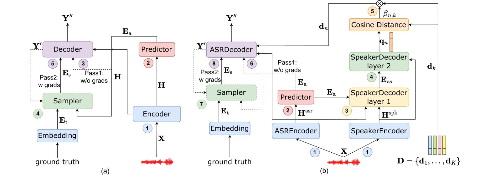
Fig. 1: (a) Structure of Paraformer. (b) Structure of the proposed SA-Paraformer.

3.1 Model architecture

Our proposed SA-Paraformer approach aims to obtain the speaker-attributed transcriptions, including transcription $\mathbf{Y}$ and speaker identity $\mathbf{S}$, given feature sequence $\mathbf{X}$ and speaker inventory $\mathbf{D}$ as input. The speaker inventory $\mathbf{D}=\{\mathbf{d}_{1},\dots,\mathbf{d}_{K}\}$ contains $K$ speaker profile vectors (e.g., d-vector [37]). The SA-Paraformer model is composed of six modules: ASREncoder, ASRDecoder, SpeakerEncoder, SpeakerDecoder, Predictor, and Sampler, as depicted in Fig. 1(b). Firstly, the ASREncoder and SpeakerEncoder are responsible for transforming the input sequence $\mathbf{X}$ into ASR hidden representation $\mathbf{H}^{\text{asr}}$ (Eq. (5)) and speaker hidden representation $\mathbf{H}^{\text{ spk }}$ (Eq. (6)), respectively. Then, the predictor module takes the ASR hidden representation $\mathbf{H}^{\text{asr}}$ as input and extracts acoustic embedding $\mathbf{E}_{\text{a}}$ corresponding to each token (Eq. (7)).

$$\mathbf{H}^{\text{ asr }}=\text{ ASREncoder }(\mathbf{X}),$$ (5)

$$\mathbf{H}^{\text{ spk }}=\text{ SpeakerEncoder }(\mathbf{X}),$$ (6)

$$\mathbf{E}_{\text{a}}=\text{ Predictor }(\mathbf{H}^{\text{ asr }}).$$ (7)

SpeakerDecoder is designed to generate a speaker profile $d_{n}$ for each token and it consists of two Transformer layers and a cosine-distance-based attention mechanism. The first Transformer layer can be described as:

$$\mathbf{E}^{\prime}_{\text{as}}=\mathbf{E}_{\text{a}}+\mathrm{MHA}^{\text{ spk-src }}\left(\mathbf{E}_{a},\mathbf{H}^{\text{ asr }},\mathbf{H}^{\text{ spk }}\right),$$ (8)

$$\mathbf{E}_{\text{as}}=\mathbf{E}^{\prime}_{\text{as}}+\mathrm{FF}^{spk}\left(\mathbf{E}^{\prime}_{\text{as}}\right).$$ (9)

Here, to obtain the speaker embedding of each token $\mathbf{E}^{\prime}_{as}$, we use $\mathbf{E}_{a}$, $\mathbf{H}^{\text{asr}}$ and $\mathbf{H}^{\text{spk}}$ as the query, key, and value of the multi-head attention (MHA) (Eq. (8)). Then, feed-forward (FF) layer receives $\mathbf{E}^{\prime}_{\text{as}}$ to obtain $\mathbf{E}_{\text{as}}$ (Eq. (9)). In the second Transformer layer, only the speaker representation $\mathbf{H}^{\text{spk}}$ is used as input, as it already contains sufficient acoustic information for each token (Eq. (10)). To obtain the speaker query $\mathbf{q}_{n}$, a linear layer is applied to adapt the dimension to the speaker inventory $\mathbf{D}$, using a learnable weight $\mathbf{W}_{\text{spk}}$ (Eq. (11)). The computation of $q_{n}$ is:

$$\mathbf{E}_{\text{spk}}=\text{TransformerLayer}\left(\mathbf{E}_{as},\mathbf{H}^{\text{spk}}\right),$$ (10)

$$\mathbf{q}_{n}=\mathbf{W}_{\text{spk}}\cdot\mathbf{E}_{\text{spk}}.\vspace{-0.1cm}$$ (11)

Then, a cosine-distance-based attention weight $\mathbf{b}_{n,k}$ is calculated between each profile $\mathbf{d}_{k}$ in the speaker inventory $\mathbf{D}$ and the obtained speaker query $\mathbf{q}_{n}$. The attention weight $\beta_{n,k}$ is derived from $\mathbf{b}_{n,k}$ through a SoftMax function. Finally, the attention-weighted speaker profile $\mathbf{d}_{n}$ is obtained by the dot product of $\beta_{n,k}$ and $\mathbf{D}$:

$$\mathbf{b}_{n,k}=\frac{\mathbf{q}_{n}\cdot\mathbf{d}_{k}}{\left|\mathbf{q}_{n}\right|\left|\mathbf{d}_{k}\right|},$$ (12)

$$\beta_{n,k}=\frac{\exp\left(\cos\left(\mathbf{b}_{n,k},\mathbf{d}_{k}\right)\right)}{\sum_{j}^{K}\exp\left(\cos\left(\mathbf{b}_{n,k},\mathbf{d}_{j}\right)\right)},$$ (13)

$${\mathbf{d}}_{n}=\sum_{k=1}^{K}\beta_{n,k}\mathbf{d}_{k}.\vspace{-0.1cm}$$ (14)

ASRDecoder inputs the acoustic embedding $\mathbf{E}_{\text{a}}$, ASR hidden representation $\mathbf{H}^{asr}$ and weighted profile ${\mathbf{d}}_{n}$ to produce the first pass hypotheses $\mathbf{Y}^{\prime}$ without backward gradients. The architecture of the ASRDecoder is similar to a Transformer decoder, except that $\mathbf{d}_{n}$ is added to the feed-forward module at the first layer (Eq. (16)).

$$\mathbf{E}^{\prime}_{c,1}=\mathbf{E}_{a}+\text{MHA}(\mathbf{E}_{a},\mathbf{H}^{\text{asr}},\mathbf{H}^{\text{asr}}),$$ (15)

$$\mathbf{E}_{c,1}=\mathbf{E}^{\prime}_{c,1}+\mathrm{FF}\left(\mathbf{E}^{\prime}_{c,1}+\mathbf{W}_{\text{spk}}\cdot\mathbf{d}_{n}\right),$$ (16)

$$\mathbf{E}_{c,l}=\text{TransformerLayer}_{l}\left(\mathbf{E}_{c,l-1},\mathbf{H}^{\text{asr}}\right),$$ (17)

$$\mathbf{Y}^{\prime}=\text{SoftMax}\left(\mathbf{W}_{\text{out}}\cdot\mathbf{E}_{c,L}+\mathbf{b}_{\text{out}}\right),\vspace{-0.1cm}$$ (18)

where $l\in\left(1,L\right)$ denotes the $l$-th layer of the ASRDecoder, $\mathbf{W}_{\text{out}}$ and $\mathbf{b}_{\text{out}}$ are learnable weight and bias parameter, $\text{Softmax}(\cdot)$ is the column-wise softmax function. Then we adopt sampler, described in Section 2, to regenerate semantic embedding $\mathbf{E}_{\text{s}}$ (Eq. (4)). Finally, ASRDecoder takes in semantic embedding $\mathbf{E}_{\text{s}}$ as well as ASR hidden representations $\mathbf{H}^{\text{asr}}$ to generate the second pass hypotheses $\mathbf{Y}^{\prime\prime}$ with backward gradients.

3.2 Speaker filling

Joint SA-ASR models, including our proposed SA-Paraformer model, are independent of the number of speakers in overlapping speech segments. But in practice, the unknown number of speakers is one of the challenges of multi-party meeting transcription, and the performance of SA-ASR models is easily affected by the number of speakers [29]. The interfering speaker (i-speaker) approach was used [29] to improve the robustness of the model for different speaker numbers, in which several interfering speaker profiles are added into speaker inventory $D$ of each utterance. However, our model uses $\mathbf{E}_{\text{a}}$ to predict speaker profiles that lack contextual information, making speaker identification more difficult. Therefore, we propose a filling speaker (f-speaker) strategy to further improve the generalization of our model by applying random disturbance. Specifically, we first expand the speaker profile number to the maximum speakers’ number of samples in a batch. Then filling the cosine distance $b_{n,k}$ of the redundant speakers with $-0.5$ to $0.5$ instead of negative infinity.

3.3 Training strategy

3.3.1 Loss function

During training, all the network parameters are optimized by four loss functions, which are MAE, cross-entropy (CE), CTC, and speaker loss. Especially, the speaker loss is added to help the model identify speakers. Thus, the final loss becomes:

$$\mathcal{L}=\mathcal{L}_{\text{M A E}}+\lambda_{1}\cdot\mathcal{L}_{\text{CTC}}+\left(1-\lambda_{1}\right)\cdot\mathcal{L}_{\text{CE}}+\mathcal{L}_{\text{spk}},\vspace{-0.1cm}$$ (19)

where $\lambda_{1}$ is an interpolation factor which is set to $0.3$ in this study. Speaker loss function $\mathcal{L}_{spk}$ is defined as:

$$\mathcal{L}_{\text{spk}}=\sum_{n}-\log\frac{e^{b_{n,i}}}{\sum_{k}e^{b_{n,k}}},\vspace{-0.1cm}$$ (20)

where $b_{n,i}$ means the cosine-distance-based attention weight of the $i$-th speaker. To further enhance the representation of the acoustic information, we introduce the inter CTC loss [36] into the intermediate layer of the acoustic encoder, expanding Eq.(19) as:

$$\begin{split}\mathcal{L}^{\prime}=\mathcal{L}_{\text{M A E}}+\lambda_{1}\cdot\mathcal{L}_{\text{CTC}}+\lambda_{2}\cdot\mathcal{L}_{\text{interCTC}}\\ +\left(1-\lambda_{1}-\lambda_{2}\right)\cdot\mathcal{L}_{\text{CE}}+\mathcal{L}_{\text{spk}},\end{split}\vspace{-0.1cm}$$ (21)

where $\lambda_{2}$ is also an interpolation factor which is set to $0.3$ in this study.

3.3.2 Token-level serialized output training (t-SOT)

Serialized output training (SOT) [9] strategy is recently proposed to generate transcriptions for multiple speakers in an effective and simple way. In the SOT strategy, transcriptions of different speakers are serialized by their start time which does not match the assumption of temporal monotonicity. Therefore, in this paper, we introduce token-level serialized output training (t-SOT) [35] strategy to enable the multi-speaker recognition ability, which is more friendly to the temporal monotonicity of CTC and Paraformer predictor in our SA-Paraformer model. The t-SOT strategy generates tokens of multiple speakers in chronological order based on token end times. However, a special token separator $\left\langle\text{cc}\right\rangle$ is inserted between tokens for channel changes, which does not contain actual acoustic information. So our proposed SA-Paraformer model is difficult to estimate the acoustic boundary of separator $\left\langle\text{cc}\right\rangle$. We experimentally investigate training our model with/without the separator $\left\langle\text{cc}\right\rangle$ in section 4.5.

4 Experiments

4.1 Datasets

We use AliMeeting corpus [12, 13], a challenging Mandarin meeting dataset with multi-talker conversations, to evaluate our proposed SA-Parafomer approach. The AliMeeting corpus contains 104.75 hours of the training set(Train), 4 hours of the evaluation set(Eval), and 10 hours of the testing set(Test). The meeting sessions of each set consist of a 15 to 30-minute discussion by a group of participants. The average speech overlap ratio of the Train set is 42.27%, which contains a number of multi-talker discussions. In this work, we use the first channel of the far-field data.

4.2 Experimental setup

In all experiments, we use the 80-dimensional Mel-filterbank feature with an 8 ms window shift and a 32 ms frame length. For the speaker profile, we employ a 256-dim Res2Net-based d-vector extractor [37] trained on the VoxCeleb corpus [38]. As we transcribe for conference audio, we got speaker profiles by clustering.

Our ASR module is comprised of 12 layers of conformer encoder [21] and 6 layers of transformer decoder. SpeakerEncoder is the same as the d-vector extractor. The dimension of attention and feed-forward layers are set to 256 and 2048, respectively. For the training process, we first trained a speaker-agnostic multi-speaker Paraformer model with the Adam optimizer. Then we use the well-trained Paraformer model and d-vector extractor as initialization. All the experiments are conducted on NVIDIA RTX 3090 GPUs and measured by speaker-dependent character error rate (SD-CER) [27], which is calculated by comparing the ASR hypothesis and the reference transcription of the corresponding speaker. We measure RTF using single-threaded bar-by-bar decoding on an Intel(R) Xeon(R) CPU E5-2678 v3 @ 2.50GHz and an NVIDIA GeForce RTX 2080 Ti, respectively.

Table 1: SD-CER of various SA-ASR approaches on Eval and Test sets. Real-time factor (RTF) is computed as the ratio of the total inference time to the total duration of the Test set.

Approach	SD-CER (%)		RTF
	Eval	Test	CPU	GPU
Cascaded SA-ASR
FD-SOT [27]	41.0	41.2	-	-
WD-SOT [27]	36.0	37.1	-	-
Joint SA-ASR
AR SA-ASR [39]	31.8	34.7	0.967	0.315
SA-Paraformer	36.2	38.6
+ interCTC	34.5	36.9
+ f-speaker	33.3	35.7	0.168	0.032
+ i-speaker	33.1	35.6
+ f&i-speaker	32.5	34.8

4.3 Comparison of different SA-ASR approaches

As shown in Table 1, our proposed SA-Paraformer approach outperforms the modular SA-ASR approaches, especially for the FD-SOT approach, leading to 11.7% (41.0% $\to$ 36.2%) and 6.3% (41.2% $\to$ 38.6%) relative SD-CER reduction on Eval and Test sets, respectively. When incorporating with inter-CTC loss, we obtain further improvement, decreasing the SD-CER from 36.2%/38.6% to 34.5%/36.9% on Eval and Test sets, respectively. The performance of SA-ASR models is easily affected by the number of speakers. Speaker filling (f-speaker) and interfering speakers (i-speaker) strategy can improve the robustness of the model with different speaker number setups. According to the results, our proposed f-speaker strategy achieves 3.4% (34.5% $\to$ 33.3%) and 3.2% (36.9% $\to$ 35.7%) relative SD-CER reduction on Eval and Test sets. And i-speaker strategy obtains similar improvements, decreasing the SD-CER from 34.5%/36.9% to 33.1%/35.6% on Eval and Test sets, respectively. Finally, combining the f-speaker and i-speaker strategy, our SA-Paraformer approach achieves a comparable SD-CER of 32.5% and 34.8% on Eval and Test sets with only 1/10 latency compared with a state-of-the-art autoregressive (AR) joint SA-ASR model which was also initialized based on a pre-trained ASR model.

4.4 Impact of the sampling factor

As shown in Table 2, we evaluate the sampling factor $\lambda$ in the sampler, described in Section 2. Here, $\lambda=0.0$ means the model training without a sampler mechanism. When increasing $\lambda$ from 0.7 to 1.1, we observe that the SD-CER is improved from 37.1% to 36.2% on the Eval set and 39.2% to 38.6% on the Test set, due to the better semantic information provided by the ground truth transcripts during training. However, when the sampling factor $\lambda$ is too large, it will lead to a mismatch between training and inference, where we decode twice with ground truth transcripts for training and decode once without transcripts for inference [34].

Table 2: Results of SA-Paraformer model with different sampling factor $\lambda$ on Eval and Test sets (SD-CER %).

$\lambda$	0.0	0.7	0.9	1.1	1.3	1.5
Eval	38.8	37.1	36.5	36.2	36.4	36.9
Test	41.1	39.2	38.8	38.6	38.7	39.0

4.5 Comparison of training with/without separator $\left\langle\text{cc}\right\rangle$

Token separator $\left\langle\text{cc}\right\rangle$ is inserted between tokens for speaker changes, which does not contain actual acoustic information. So, the predictor of our SA-Paraformer model, based on acoustic boundary estimation, is difficult to deal with the separator $\left\langle\text{cc}\right\rangle$. As shown in Table 3, we compared the CER detailed results of the SA-Paraformer model training with (A1 model) and without (A2 model) the separator $\left\langle\text{cc}\right\rangle$. Compared with the A1 model, the A2 model brings 10.4% (43.1% $\to$ 38.6%) relative CER reduction on the Test set, due to the decreasing of deletion (Del) errors (26.5% $\to$ 6.5%). As can be seen from Fig 2, the upper part shows the ground truth sequence and the middle part shows the A1 model inference sequence. After analyzing the decoding results, we find that most of the deletion errors of the A1 model are the normal token. For the utterance of multi-speaker discussion, the A1 model outputs separator $\left\langle\text{cc}\right\rangle$ and ignores normal token. We remove the separator during training to improve the prediction accuracy of the normal token boundary for recovering the deletion errors. As shown in the lower part of Fig. 2, the deletion error of the normal token is successfully corrected.

Table 3: Results of training with/without separator on Test set (CER %).

Model	With separator	Ins	Del	Sub	CER
A1	Yes	3.4	26.4	13.3	43.1
A2	No	4.2	6.8	27.6	38.6

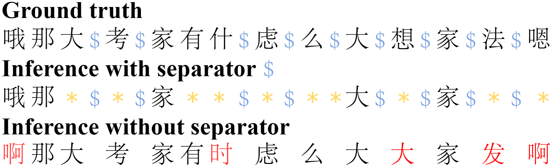
Fig. 2: Decoding example for R8002-MS802-0004385-0004672 in the AliMeeting Test set. Red indicates substitution error and yellow indicates deletion error.

5 Conclusion

In this paper, we propose an SA-Paraformer model based on the multi-speaker t-SOT framework to transcribe speech and identify speakers simultaneously, which introduces the Paraformer non-autoregressive model as an acoustic model for parallel decoding. Besides, we also propose a simple strategy speaker filling to improve the robustness of the model with different speaker number. Finally, we introduce the interfering speakers and inter-CTC strategy to obtain further improvement. Evaluated on the AliMeeting corpus, our proposed SA-Paraformer model achieves 6.1% relative SD-CER improvement compared with the cascaded SA-ASR model on the test set. Moreover, the SA-Paraformer model achieves a comparable SD-CER of 34.8% to the state-of-the-art autoregressive joint SA-ASR model with 30 times speedup on GPU. In the future, we would like to integrate a multi-channel model into our proposed SA-Paraformer model for real-world applications.

References

- [1] J. G. Fiscus, J. Ajot, M. Michel, and J. S. Garofolo, “The rich transcription 2006 spring meeting recognition evaluation,” in Proc. MLMI. Springer, 2006, pp. 309–322.
- [2] J. G. Fiscus, J. Ajot, and J. S. Garofolo, “The rich transcription 2007 meeting recognition evaluation,” in Proc. MTPH. Springer, 2007, pp. 373–389.
- [3] J. Barker, S. Watanabe, E. Vincent, and J. Trmal, “The fifth ’CHiME’ speech separation and recognition challenge: Dataset, task and baselines,” in Proc. INTERSPEECH. ISCA, 2018, pp. 1561–1565.
- [4] S. Watanabe, M. Mandel, J. Barker et al., “CHiME-6 challenge: Tackling multispeaker speech recognition for unsegmented recordings,” CoRR, vol. abs/2004.09249, 2020.
- [5] N. Ryant, P. Singh, V. Krishnamohan, R. Varma, K. Church, C. Cieri, J. Du, S. Ganapathy, and M. Liberman, “The third DIHARD diarization challenge,” in Proc. INTERSPEECH. ISCA, 2021, pp. 3570–3574.
- [6] I. McCowan, J. Carletta, W. Kraaij, S. Ashby, S. Bourban, M. Flynn et al., “The AMI meeting corpus,” in Proc. ICMT, vol. 88. Citeseer, 2005, p. 100.
- [7] D. Yu, X. Chang, and Y. Qian, “Recognizing multi-talker speech with permutation invariant training,” in Proc. INTERSPEECH. ISCA, 2017, pp. 2456–2460.
- [8] Z. Chen, J. Droppo, J. Li, and W. Xiong, “Progressive joint modeling in unsupervised single-channel overlapped speech recognition,” IEEE ACM Trans. Audio Speech Lang. Process., vol. 26, no. 1, pp. 184–196, 2018.
- [9] N. Kanda, Y. Gaur, X. Wang, Z. Meng, and T. Yoshioka, “Serialized output training for end-to-end overlapped speech recognition,” in Proc. INTERSPEECH. ISCA, 2020, pp. 2797–2801.
- [10] P. Guo, X. Chang, S. Watanabe, and L. Xie, “Multi-speaker ASR combining non-autoregressive Conformer CTC and conditional speaker chain,” in Proc. INTERSPEECH. ISCA, 2021, pp. 3720–3724.
- [11] F. Yu, S. Zhang, P. Guo, Y. Liang, Z. Du, Y. Lin, and L. Xie, “MFCCA:multi-frame cross-channel attention for multi-speaker asr in multi-party meeting scenario,” in Proc. SLT. IEEE, 2023, pp. 144–151.
- [12] F. Yu, S. Zhang, Y. Fu, L. Xie, S. Zheng, Z. Du et al., “M2MeT: The ICASSP 2022 multi-channel multi-party meeting transcription challenge,” in Proc. ICASSP. ISCA, 2022, pp. 6167–6171.
- [13] F. Yu, S. Zhang, P. Guo, Y. Fu, Z. Du, S. Zheng, L. Xie et al., “Summary on the ICASSP 2022 multi-channel multi-party meeting transcription grand challenge,” in Proc. ICASSP. ISCA, 2022, pp. 9156–9160.
- [14] D. Yu, M. Kolbæk, Z.-H. Tan, and J. Jensen, “Permutation invariant training of deep models for speaker-independent multi-talker speech separation,” in Proc. ICASSP. ISCA, 2017, pp. 241–245.
- [15] J. R. Hershey, Z. Chen, J. Le Roux, and S. Watanabe, “Deep clustering: Discriminative embeddings for segmentation and separation,” in Proc. ICASSP. ISCA, 2016, pp. 31–35.
- [16] Z. Chen, Y. Luo, and N. Mesgarani, “Deep attractor network for single-microphone speaker separation,” in Proc. ICASSP. ISCA, 2017, pp. 246–250.
- [17] T. J. Park, N. Kanda, D. Dimitriadis, K. J. Han, S. Watanabe, and S. Narayanan, “A review of speaker diarization: Recent advances with deep learning,” Proc. CSL, vol. 72, p. 101317, 2022.
- [18] Y. Fujita, N. Kanda, S. Horiguchi, Y. Xue, K. Nagamatsu, and S. Watanabe, “End-to-end neural speaker diarization with self-attention,” in Proc. ASRU. IEEE, 2019, pp. 296–303.
- [19] S. Horiguchi, Y. Fujita, S. Watanabe, Y. Xue, and K. Nagamatsu, “End-to-end speaker diarization for an unknown number of speakers with encoder-decoder based attractors,” in Proc. INTERSPEECH. ISCA, 2020, pp. 269–273.
- [20] A. Vaswani, N. Shazeer, N. Parmar, J. Uszkoreit, L. Jones, A. N. Gomez, L. Kaiser, and I. Polosukhin, “Attention is all you need,” in Proc. NeurIPS, 2017, pp. 5998–6008.
- [21] A. Gulati, J. Qin, C.-C. Chiu, N. Parmar et al., “Conformer: Convolution-augmented transformer for speech recognition,” in Proc. INTERSPEECH. ISCA, 2020, pp. 5036–5040.
- [22] J. Li, “Recent advances in end-to-end automatic speech recognition,” CoRR, vol. abs/2111.01690, 2021.
- [23] Z. Chen, T. Yoshioka, L. Lu, T. Zhou, Z. Meng, Y. Luo, J. Wu, X. Xiao, and J. Li, “Continuous speech separation: Dataset and analysis,” in Proc. ICASSP. ISCA, 2020, pp. 7284–7288.
- [24] X. Chang, W. Zhang, Y. Qian, J. Le Roux, and S. Watanabe, “MIMO-Speech: End-to-end multi-channel multi-speaker speech recognition,” in Proc. ASRU. IEEE, 2019, pp. 237–244.
- [25] W. Zhang, C. Boeddeker, S. Watanabe, Y. Qian et al., “End-to-end dereverberation, beamforming, and speech recognition with improved numerical stability and advanced frontend,” in Proc. ICASSP. ISCA, 2021, pp. 6898–6902.
- [26] J. Wu, Z. Chen, J. Li, T. Yoshioka, Z. Tan et al., “An end-to-end architecture of online multi-channel speech separation,” in Proc. INTERSPEECH. ISCA, 2020, pp. 81–85.
- [27] F. Yu, Z. Du, S. Zhang, Y. Lin, and L. Xie, “A comparative study on speaker-attributed automatic speech recognition in multi-party meetings,” in Proc. INTERSPEECH. ISCA, 2022, pp. 560–564.
- [28] N. Kanda, X. Chang, Y. Gaur, X. Wang, Z. Meng, Z. Chen et al., “Investigation of end-to-end speaker-attributed ASR for continuous multi-talker recordings,” in Proc. SLT. IEEE, 2021, pp. 809–816.
- [29] N. Kanda, Y. Gaur, X. Wang, Z. Meng, Z. Chen, T. Zhou, and T. Yoshioka, “Joint speaker counting, speech recognition, and speaker identification for overlapped speech of any number of speakers,” in Proc. INTERSPEECH. ISCA, 2020, pp. 36–40.
- [30] N. Kanda, X. Xiao, J. Wu, T. Zhou, Y. Gaur, X. Wang, Z. Meng, Z. Chen, and T. Yoshioka, “A comparative study of modular and joint approaches for speaker-attributed ASR on monaural long-form audio,” in Proc. ASRU. IEEE, 2021, pp. 296–303.
- [31] N. Kanda, G. Ye, Y. Gaur, X. Wang, Z. Meng, Z. Chen, and T. Yoshioka, “End-to-end speaker-attributed ASR with Transformer,” in Proc. INTERSPEECH. ISCA, 2021, pp. 4413–4417.
- [32] Y. Higuchi, S. Watanabe, N. Chen, T. Ogawa, and T. Kobayashi, “Mask CTC: Non-autoregressive end-to-end ASR with CTC and mask predict,” in Proc. INTERSPEECH. ISCA, 2020, pp. 3655–3659.
- [33] L. Dong and B. Xu, “CIF: Continuous integrate-and-fire for end-to-end speech recognition,” in Proc. ICASSP. ISCA, 2020, pp. 6079–6083.
- [34] Z. Gao, S. Zhang, I. McLoughlin, and Z. Yan, “Paraformer: Fast and accurate parallel Transformer for non-autoregressive end-to-end speech recognition,” in Proc. INTERSPEECH. ISCA, 2022, pp. 5079–5083.
- [35] N. Kanda, J. Wu, Y. Wu, X. Xiao, Z. Meng, X. Wang, Y. Gaur, Z. Chen, J. Li, and T. Yoshioka, “Streaming multi-talker ASR with token-level serialized output training,” in Proc. INTERSPEECH. ISCA, 2022, pp. 3774–3778.
- [36] J. Lee and S. Watanabe, “Intermediate loss regularization for CTC-based speech recognition,” in Proc. ICASSP. ISCA, 2021, pp. 6224–6228.
- [37] E. Variani, X. Lei, E. McDermott, I. L. Moreno, and J. Gonzalez-Dominguez, “Deep neural networks for small footprint text-dependent speaker verification,” in Proc. ICASSP. ISCA, 2014, pp. 4052–4056.
- [38] A. Nagrani, J. S. Chung, and A. Zisserman, “Voxceleb: A large-scale speaker identification dataset,” in Proc. INTERSPEECH. ISCA, 2017, pp. 2616–2620.
- [39] M. Shi, Z. Du, Q. Chen, F. Yu, Y. Li, S. Zhang, J. Zhang, and L.-R. Dai, “Casa-asr: Context-aware speaker-attributed asr,” in Proc. INTERSPEECH. ISCA, 2023.