Supplementary Material for “Optical Trapping of Large Metallic Particles in Air”

I Generation of Uniform Transverse Intensity Distribution of Scanning Laser

As noted in the main text, the scan speed of the laser must be constant along its parabolic path to generate a uniform quasistatic intensity distribution. Here we give details on how this is accomplished.

The laser beam is linearly polarized in the $z$-direction and propagating in the $+x$ direction. Denoting the scanning frequency is $\omega$, we may write the time-averaged intensity over the time period $T=\frac{2\pi}{\omega}$ as: $I_{ave}(\vec{r})=\frac{1}{T}\int_{0}^{T}I(x,y,z;t)dt$, where $\left(y_{f}(t),z_{f}(t)\right)=(d\sin(\omega t),-d\cos(2\omega t))$ and $\dot{s}(t)=d\omega\sqrt{\cos^{2}(\omega t)+4\sin^{2}(2\omega t)}$ is the speed of scanner. Figure S1(a) shows an example time-averaged non-uniform intensity in the $x=0$ plane, where the simulation parameters are chosen as follows: $\lambda=$ 532 nm, $p_{in}=10$ mW, $NA=0.2$, $\omega=5$ kHz, and $d=5$ $\mu$m. For this intensity distribution, the speed of the scanner is not constant along the parabolic path which would result in a non-uniform distribution, as seen in Fig. S1(a). As shown experimentally, the intensity distribution significantly affects the quality of trapping. In the non-uniform case, the lateral walls have a lower average intensity compared to the other parts. Thus, the particles are more likely to leave the trap region from the low-intensity regions before being re-illuminated by the scanning laser beam.

To overcome this limitation, we create a uniform intensity distribution by using a constant speed for the scanner along the parabolic path. If the scan rate for uniform distribution is the same as the non-uniform case, the speed of the scanner in the uniform distribution is $v=\frac{2s_{tot}}{T}$, in which $s_{tot}=\int_{0}^{T/2}\dot{s}(t)dt$ is the total traveled distance on the parabola path, and $s(t)$ is the position of laser beam at time $t$. To obtain the uniform distribution, a different time scale $t^{{}^{\prime}}(t)$ should be used, related to the time scale of the non-uniform distribution $t$ as follows:

$$vt^{{}^{\prime}}=\int_{0}^{t}\dot{s}(\tau)d\tau.$$ (S1)

Then, the uniform time-averaged intensity reads

$$I_{ave}(\vec{r})=\frac{1}{t^{\prime}(T)}\int_{0}^{t^{\prime}(T)}I\left(\vec{r};t^{\prime}(t)\right)dt^{\prime}.$$ (S2)

The uniform time-averaged intensity distribution is shown in Fig. S1(b). The distributed intensities located on the opposite sides of the parabola converge on the back ($x<0$) and front sides ($x>0$) in the axial direction as shown in Fig. S1(c).

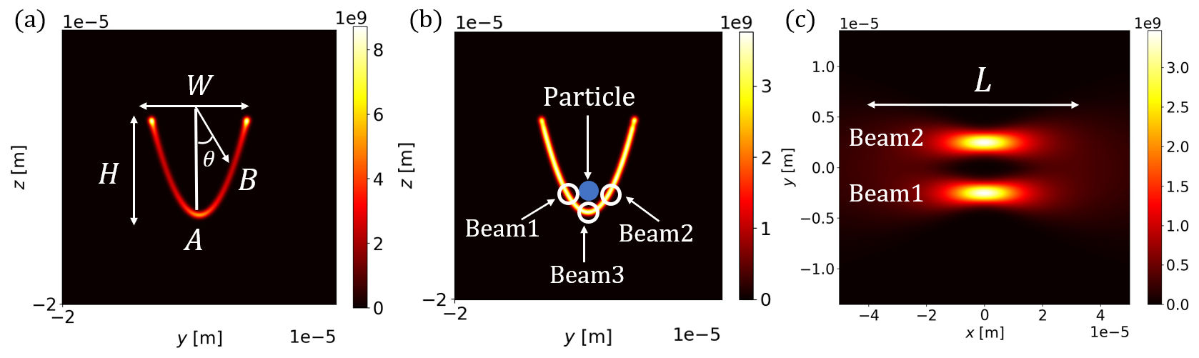
Fig. S1: (a) The non-uniform and (b) uniform time-averaged intensity distribution in the transverse plane at $x=0$. (c) The convergence of beams 1 and 2 along the axial direction.

II Optical and thermal forces calculations

The optical forces are calculated using Maxwell stress tensor (MST) Novotny and Hecht (2012). We first calculate MST ($\bar{\bar{T}}$) by finding the macroscopic electromagnetic field components (incident and scattering) on a closed surface $\partial v$ surrounding the particle.

$$\bar{\bar{T}}=\varepsilon_{0}\varepsilon_{r}\vec{E}\vec{E}+\mu_{0}\mu_{r}\vec{H}\vec{H}-\frac{1}{2}\left(\varepsilon_{0}\varepsilon_{r}|\vec{E}|^{2}+\mu_{0}\mu_{r}|\vec{H}|^{2}\right)\bar{\bar{I}}$$ (S3)

where $\vec{E}$ and $\vec{H}$ are the macroscopic electric and magnetic fields, respectively, and $\bar{\bar{I}}$ is the unit tensor. Then, we calculate the time-average force $\langle\vec{F}(\vec{r},t)\rangle$ by integrating MST over $\partial v$.

$$\langle\vec{F}_{opt}(\vec{r},t)\rangle=\oint\langle\bar{\bar{T}}(\vec{r},t)\rangle.\hat{n}(\vec{r})ds$$ (S4)

where $\hat{n}$ is the upward unit vector perpendicular to the surface. We use COMSOL Multiphysics to implement and calculate MST.

To model the photophoretic force, we note that the mean free path of the surrounding air particles is much smaller than the radius of the trapped particles, allowing us to model photophoretic force in the continuous regime with appropriate boundary conditions. We first find the temperature distribution on the particle’s surface using the heat transfer equation:

$$\vec{\nabla}.\left(\kappa\vec{\nabla}T(\vec{r},t)\right)+Q(\vec{r})=\rho c_{p}\partial_{t}T(\vec{r},t)$$ (S5)

where $\kappa$ is thermal conductivity, $T$ is temperature, $\rho$ is mass density, and $c_{p}$ is specific heat capacity. The volumetric heat source $Q$ is related to the electromagnetic radiation by $Q(\vec{r})=2\pi f\varepsilon_{0}\varepsilon_{r}^{{}^{\prime\prime}}I_{ave}(\vec{r})$, where $f$ is laser frequency, and $\varepsilon_{r}^{{}^{\prime\prime}}$ is the imaginary part of the particle’s permittivity. We next apply two boundary conditions to solve the heat transfer equation: absorption of the laser illumination from a given direction, and cooling through thermal emission in all directions. By combining these boundary conditions, we obtain the Neumann boundary condition

$$\kappa\vec{\nabla}T\cdot\hat{n}=I_{ave}\hat{x}\cdot\hat{n}-\sigma\epsilon(T^{4}-T_{0}^{4}),$$ (S6)

where $T_{0}=20$ ^∘C is the ambient temperature, $\sigma$ is the Stefan-Boltzmann constant and $\epsilon$ is emissivity that we set $\epsilon=0.8$. The radius and refractive index of gold particles are $R=500$ nm and $\tilde{N}=0.543+j2.2309$, respectively, and the mean free path of the air at $P=1$ atm is approximately $69.4$ nm, which results in a Knudsen number of $K_{n}=0.069$. The photophoretic force can be calculated by integrating the inhomogeneous temperature over the particle’s surface Zulehner and Rohatschek (1995)

$$\vec{F}_{ph}=-\left(\frac{\alpha P}{4T_{0}}\right)\oint T(\vec{r})\hat{n}ds,$$ (S7)

where $\alpha$ is thermal accommodation. The total force $\vec{F}_{tot}$ is calculated as the sum of the optical force $\vec{F}_{opt}$, the photophoretic force $\vec{F}_{ph}$ and the gravitational force $\vec{F}_{gr}$. To simplify this calculation, we take advantage of the trap symmetry in the transverse $y-z$ plane and the assumption that the quasistatic intensity distribution profile is constant along the parabolic path. The sum of the optical and photophoretic forces $\vec{F}_{opt}$+$\vec{F}_{ph}$ may be found using one force calculation, since the magnitude $\mid\vec{F}_{opt}\mid\ +\mid\vec{F}_{ph}\mid$ is a constant at all points along the parabola, but with a different direction at each point. We calculate the sum of optical and photophoretic forces $\vec{F}_{A}$ at a point $A=(x,0,z)$ on the $y=0$ plane and apply a rotation matrix $\bar{\bar{R}}(\theta)$ to find the sum of optical and photophoretic forces $\vec{F}_{B}$ at a point $B=(x,y(\theta),z(\theta))$:

$$\vec{F}_{B}=\bar{\bar{R}}(\theta)\vec{F}_{A}=\begin{bmatrix}1&0&0\\ 0&\cos(\theta)&-\sin(\theta)\\ 0&\sin(\theta)&\cos(\theta)\end{bmatrix}\begin{bmatrix}F_{x}\\ F_{y}\\ F_{z}\end{bmatrix},\hskip 2.84544pt-\frac{\pi}{2}\leq\theta\leq\frac{\pi}{2}$$ (S8)

where $\vec{F}_{A}=\left[F_{x}F_{y}F_{z}\right]^{T}$ and $(y(\theta),z(\theta))=(d\sin(\theta),-d\cos(2\theta))$. The points $A$, $B$, and angle $\theta$ are specified in Figure S1(a). Figure S2(a) and S2(b) show the intensity profile and temperature distribution of the particle’s surface at the same point $A$, which are calculated using COMSOL Multiphysics. In this example, the bottom of the particle is closer to the high-intensity region than the top of the particle, resulting in a higher temperature on the bottom and a photophoretic force in the $+z$ direction.

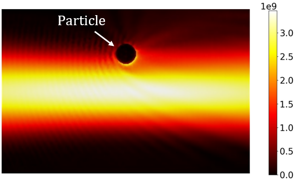
(a)

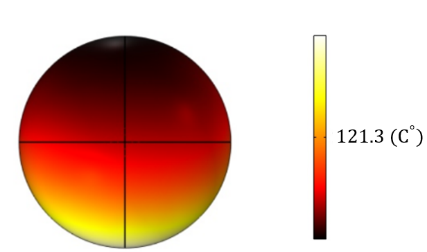
(b)

Fig. S2: (a) The intensity profile of a single laser beam, where a gold microparticle is located on top of the intensity barrier. (b) The temperature distribution on the surface of the particle.

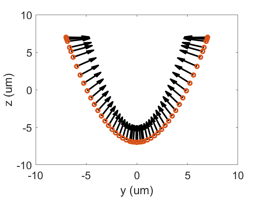
(a)

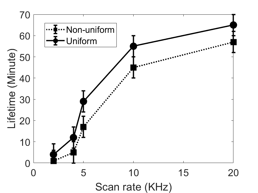
(b)

Fig. S3: (a) The vector map of the total force in the transverse plane. (b) The trapping lifetime as a function of scan rate. The solid line shows the lifetime for uniform intensity distribution and the dashed line is the lifetime of the non-uniform intensity distribution.

The vector map of the total force in the transverse plane is shown in Fig. 3(a). The red circles show the position of the particle on the parabola path and the black arrows indicate the direction and relative magnitudes of the total force.

The mean trapping lifetime as a function of scan rate is shown in Fig. 3(b). Each data point represents the average of 10 experiments, and the bars indicate the standard deviation. By increasing the scan rate, the lifetime is increased. Moreover, the uniformly distributed intensity beams show better performance than the non-uniform distribution. As shown in the uniform distribution lifetimes beyond 1 hour are achieved at $20$ kHz

The trapping locus can easily move in three-dimensional space by shifting the range of the tuning voltage of the VCO. In Fig. S4 the translation of the boat trap along the axial direction is shown for a uniform distribution at 10 kHz. After the particle was stably trapped at the first point, the boat trap site was moved to another location. Consequently, the particle is moved to the second stable point in the axial direction.

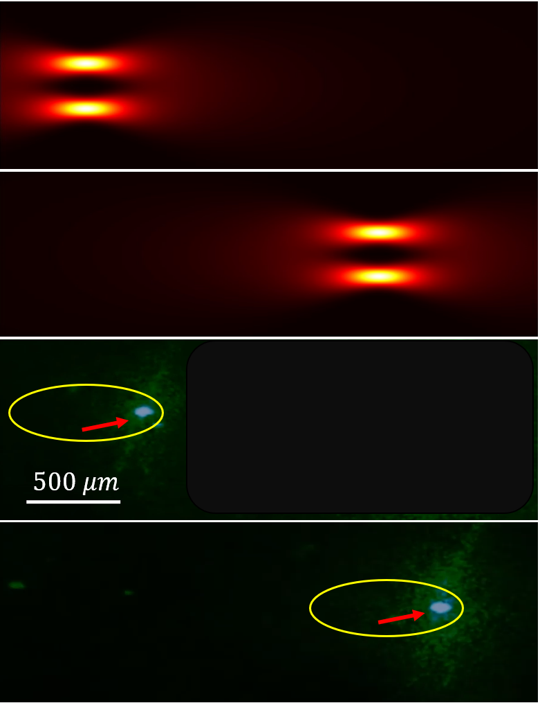
Fig. S4: (a) The translation operation for uniform distribution at $10$ kHz.

References

- Novotny and Hecht (2012) L. Novotny and B. Hecht, Principles of nano-optics (Cambridge university press, 2012).
- Zulehner and Rohatschek (1995) W. Zulehner and H. Rohatschek, Journal of aerosol science 26, 201 (1995).