On changepoint detection in functional data using empirical energy distance

Abstract.

We propose a novel family of test statistics to detect the presence of changepoints in a sequence of dependent, possibly multivariate, functional-valued observations. Our approach allows to test for a very general class of changepoints, including  the “classical” case of changes in the mean, and even changes in the whole distribution. Our statistics are based on a generalisation of the empirical energy distance; we propose weighted functionals of the energy distance process, which are designed in order to enhance the ability to detect breaks occurring at sample endpoints. The limiting distribution of the maximally selected version of our statistics requires only the computation of the eigenvalues of the covariance function, thus being readily implementable in the most commonly employed packages, e.g. R. We show that, under the alternative, our statistics are able to detect changepoints occurring even very close to the beginning/end of the sample. In the presence of multiple changepoints, we propose a binary segmentation algorithm to estimate the number of breaks and the locations thereof. Simulations show that our procedures work very well in finite samples. We complement our theory with applications to financial and temperature data.

1. Introduction

The analysis of datasets where the data are observed as functions, rather than scalars or vectors, has been investigated in numerous contributions over the past few years. Functional Data Analysis (FDA) has become ubiquitous in virtually all applied sciences, in the case where data are genuinely functional in nature, and also when a parsimonious description of the data is called for. FDA appears naturally in the analysis of economic and financial data; examples include analysing the term structure of interest rates, where, for each time period, the observed maturities are the discrete approximation of the continuum of maturities (Hays et al., 2012); and modelling intraday return density trajectories (Bathia et al., 2010). In climate science, it is typical to model temperatures - which are recorded at a high frequency basis, e.g. several times per day - at a lower frequency (e.g. yearly), with the intra-period data representing the discretised functional observations - see, for example, Horváth and Kokoszka (2012) and King et al. (2018). In medical imaging, several datasets arise that can be modelled as possibly multi-dimensional and functional valued (Sørensen et al., 2013). See also Ramsay and Silverman (2002) for further examples.

On account of the huge relevance of the topic, inferential theory for FDA has been studied in many contributions. The literature has developed useful dimension reduction tools such as the functional version of Principal Components (Hall et al., 2006), and the full-blown estimation theory for linear regression, dynamic models and also nonlinear models such as the functional version of ARCH and GARCH (Horváth and Kokoszka, 2012). However, the validity of inferential theory often hinges on having some stability in the structure of the data, such as the constancy of the mean function, or of the whole distribution. Hence, testing for the possible presence of changepoints (in the mean, in higher order moments, or even in the whole distribution) is of paramount importance.

Changepoint detection is well-studied in the context of scalar or vector-valued time series, and we refer, inter alia, to Casini and Perron (2019) for a useful review containing several examples and applications. In contrast, changepoint analysis in functional data has received only limited attention. Berkes et al. (2009) propose a CUSUM-based test statistic to detect changepoints in the mean of independent functional-valued observations; Hörmann and Kokoszka (2010), Zhang et al. (2011), Aston and Kirch (2012) and Aue et al. (2018) consider extensions to deal with dependent data, which typically occur in a time series context. These contributions, broadly speaking, are based on the unweighted CUSUM process, and it is possible to show that, in this case, $N^{1/2}$ periods away from the beginning/end of the sample (where $N$ is the sample size). On the other hand, detection of early/late occurring breaks is very important, due to its implications on the ability to assess timely whether a model which has been valid so far is still appropriate e.g. for forecasting.

Main contributions of this paper

In this paper, we bridge the gaps discussed above, by proposing a procedure to detect changepoints for serially dependent, possibly multivariate functional-valued time series, allowing for breaks to occur close to the sample endpoints. We consider very general changes, which could occur in various functions/functionals of the data, including the mean, higher order moments, and in general functions which completely characterize the underlying distribution such as the characteristic function. Specifically, we develop a novel family of weighted test statistics based on the notion of energy distance (see e.g. Székely and Rizzo, 2005; Székely and Rizzo, 2017; and Baringhaus and Franz, 2004). The energy distance is a metric designed to measure the distance between the distributions of two independent random vectors (say $X$ and $Y$), defined as

(1.1) $$\mathcal{E}_{\eta}(X,Y)=2E\left|X-Y\right|^{\eta}-E\left|X-X^{\prime}\right|^{\eta}-E\left|Y-Y^{\prime}\right|^{\eta},$$

where $X^{\prime},Y^{\prime}$ are independent copies of $X$ and $Y$, respectively, $\left|\cdot\right|$ is the Euclidean norm, and $0<\eta<2$; it can be shown (see Theorem 2 in Székely and Rizzo, 2005) that $\mathcal{E}_{\eta}(X,Y)=0$ if and only if $X$ and $Y$ have the same distribution. Empirical energy distances have been used by Matteson and James (2014) and Biau et al. (2016) to study distributional changepoint problems for a sequence of independent, vector-valued time series; Chakraborty and Zhang (2021) extend the theory to the case of high-dimensional sequences.

Taking $\eta=2$ in (1.1) leads to a statistic suitable for testing equality of expectations rather than equality of distributions (Székely and Rizzo, 2005). Hence, we consider an empirical version of $\mathcal{E}_{2}(X,Y)$, constructed at every point in the sample $1\leq k\leq N$, comparing the sample average before and after $k$ in a (conceptually) similar way to the CUSUM process. We then consider weighted versions of the empirical energy process, with weights designed to boost the value taken by the process when $k$ is close to the beginning/end of the sample. Changepoint detection can thus be based on the maximally selected weighted empirical energy process. The resulting tests have nontrivial power versus breaks occurring (much) closer to the sample endpoints than $N^{1/2}$ periods, while still having power versus mid-sample breaks. In Section 3 we show that the limiting distribution of our test statistics contains the integral of the square of a Gaussian process which depends - in a highly nontrivial way - on nuisance parameters. Hence, in order to compute critical values, we propose a method based on the Karhunen-Loève (KL henceforth) expansion, which appears to be easier to use than e.g. the bootstrap (see e.g., albeit in a different context, Inoue, 2001). Our theory is stated for the general case of multivariate functional time series whose argument can also be multivariate, which is relevant in several applications of FDA, including shape analysis (Kenobi et al., 2010) and medical imaging (Kurtek et al., 2010).

For the sake of clarity, our presentation focuses mainly on detecting changes in the mean of functional observations. However, our approach can be readily applied to consider different changepoint problems; in Section 4 we discuss how our tests can be used to detect distributional changes, by applying it to the empirical characteristic function. Testing for changes in the distribution is arguably of great importance; as Inoue (2001) puts it, “[…] stability of distribution, moments, or parameters is essential to the proofs of asymptotic properties of the maximum likelihood method, generalized method of moments, and nonparametric method. Consequently, instability can affect estimation and inference.” (p. 156). Contributions on this topic often require independence assumptions, and are relatively scarce even in the case of scalar or vector-valued observations: in addition to the papers by Matteson and James (2014) and others referred to above, other approaches include Inoue (2001), who uses the unweighted CUSUM process based on the empirical distribution function; Antoch et al. (2008), who use a combination of rank statistics; and Hušková and Meintanis (2006), who use the empirical characteristic function for scalar observations.

The remainder of the paper is organised as follows. We present our test statistics in Section 2. We study its asymptotic theory in Section 3: we derive the weak limit under the null in Section 3.1; we study power, estimation of the breakdate, and binary segmentation in Section 3.2; we offer a methodology to compute critical values in Section 3.3. We extend our approach to detecting changes in the distribution of the data is in Section 4. In Section 5, we report a comprehensive simulation exercise; an empirical application to intraday returns is in Section 6. Section 7 concludes. Further Monte Carlo evidence, an empirical application to temperature data, lemmas and proofs are relegated to the Supplement.

NOTATION. Henceforth, $\mathcal{T}$ denotes a compact subset of $\mathbb{R}^{d}$, and $\{x(t),\leavevmode\nobreak\ t\in\mathcal{T}\}$ is a square integrable function; whenever convenient, we write $x$ in place of $x(t)$ or in place of $\{x(t),\leavevmode\nobreak\ t\in\mathcal{T}\}$. For any $r\geq 1$, given two square integrable $\mathbb{R}^{r}$-valued functions $\{x(t),\leavevmode\nobreak\ t\in\mathcal{T}\}$ and $\{y(t),\leavevmode\nobreak\ t\in\mathcal{T}\}$, we define the inner product $\langle x,y\rangle=\int_{\mathcal{T}}x^{\top}(t)y(t)dt$, where “^⊤” is the usual transpose; and we define the $L^{2}$-norm $\|x\|=\sqrt{\langle x,x\rangle}$, writing $x=y$ if $\|x-y\|=0$. When unambiguous, we write $\{a_{\ell}\}$ to denote a given sequence $\{a_{\ell},-\infty<\ell<\infty\}$. We also write the symbol $\int$ in place of $\int_{\mathcal{T}}$. We use: “$\underset{\mathcal{D}[0,1]}{\overset{w}{\longrightarrow}}$” to denote weak convergence in $\mathcal{D}[0,1]$; “$\overset{{\mathcal{D}}}{\rightarrow}$” to denote convergence in distribution; “$\overset{\mathcal{P}}{\rightarrow}$” for convergence in probability; “a.s.” for “almost surely”; “$\overset{{\mathcal{D}}}{=}$” for equality in distribution; $\lfloor\cdot\rfloor$ for the integer value function; and $\left|\cdot\right|$ to denote the Euclidean norm of a vector, or the Frobenius norm of a matrix. Other relevant notation is introduced further in the paper.

2. The test statistics: definition, assumptions and asymptotics

We consider a sequence of $\mathbb{R}^{r}$-valued functional observations of the form

$$X_{i}(t)=\mu_{i}(t)+\epsilon_{i}(t),\qquad t\in\mathcal{T\subset}\mathbb{R}^{d},\quad 1\leq i\leq N,$$

where for each $i$, $\mu_{i}$ and $\epsilon_{i}$ are $\mathbb{R}^{r}$-valued square integrable functions. We aim to test

(2.1) $$H_{0}:\mu_{1}=\mu_{2}=\ldots=\mu_{N},$$

against the $R$-change alternative:

(2.2) $$H_{A}:\text{there are $1<k_{1}<\ldots<k_{R}<N$ s.t. }\|\mu_{k_{i}+1}-\mu_{k_{i}}\|>0,\quad\mu_{k_{i-1}+1}=\ldots=\mu_{k_{i}},$$

for $i=1,\ldots,R$, with the convention that $k_{0}=1$ and $k_{R+1}=N$.

As discussed in the introduction, a possible way of detecting changes is based on the energy distance defined in (1.1). Our approach is based on weighted functionals of $\{V_{N}(k),\,2\leq k\leq N-2\}$, defined as the empirical version of the energy distance calculated for $\eta=2$

(2.3) $$V_{N}(k)=\frac{2}{k(N-k)}\sum_{i=1}^{k}\sum_{j=k+1}^{N}\|X_{i}-X_{j}\|^{2}-\frac{1}{\displaystyle{{\binom{k}{2}}}}\sum_{1\leq i<j\leq k}\|X_{i}-X_{j}\|^{2}-\frac{1}{\displaystyle{{\binom{N-k}{2}}}}\sum_{k<i<j\leq N}\|X_{i}-X_{j}\|^{2}.$$

Throughout the paper, we assume that the sequence $\{X_{i}\}$ is weakly dependent:

Assumption 2.1.

(i) the sequence $\{\epsilon_{\ell},-\infty<\ell<\infty\}$ is a Bernoulli shift sequence, i.e., it has the representation $\epsilon_{\ell}=g(\eta_{\ell},\eta_{\ell-1},\ldots)$, where for each $\ell$, $\eta_{\ell}=\eta_{\ell}(t,\omega)$ are i.i.d. functions jointly measurable in $(t,\omega)$ taking values in a measurable space $\mathcal{S}$, and $g$ is a nonrandom measurable function $g:\mathcal{S}^{\infty}\rightarrow L^{2}(\mathcal{T})$; (ii) $E\epsilon_{1}(t)=0$ and $E\|\epsilon_{1}\|^{{4+\epsilon}}<\infty$ with some ${\epsilon}>0$; (iii) for some $\kappa>{4+\epsilon}$, $\sum_{m=1}^{\infty}\big{(}E\|\epsilon_{1}-\epsilon_{1}^{(m)}\|^{{4+\epsilon}}\big{)}^{1/\kappa}<\infty$, where for each pair $(j,\ell)$, we set $\epsilon_{\ell}^{(j)}=g(\eta_{\ell},\eta_{\ell-1},\ldots,\eta_{\ell-j+1},\eta_{\ell-j}^{(j)},\eta_{\ell-j-1}^{(j)},\ldots)$, with $\{\eta_{\ell}^{(j)},-\infty<\ell<\infty\}$ an independent copy of $\{\eta_{\ell},-\infty<\ell<\infty\}$.

Assumption 2.1 states that the sequence $\{\epsilon_{\ell},\leavevmode\nobreak\ -\infty<\ell<\infty\}$ is stationary and ergodic, and it can be approximated by a sequence with finite-order dependence (see Hörmann and Kokoszka, 2010). The Bernoulli shift representation in Assumption 2.1 is widely employed in the analysis of scalar time series, where it can be verified in the most commonly used DGPs in econometrics and statistics. As far as functional-valued data are concerned, examples when Assumption 2.1 hold include linear processes in Hilbert spaces (Horváth and Kokoszka, 2012), and a large class of non-linear processes, including functional ARCH and GARCH models (Aue et al., 2017) and bilinear models (Hörmann and Kokoszka, 2010).

3. Asymptotics

We will consider the following statistics:

(3.1) $$\frac{1}{2}N\left(u\left(1-u\right)\right)^{2-\alpha}V_{N}\left(\left\lfloor Nu\right\rfloor\right),\quad 2/N\leq u\leq 1-2/N,$$

where $0\leq\alpha<1$ and $u=k/N$. A full-blown discussion is after Theorems 3.1 and 3.2 below; here we offer a heuristic preview of the rationale of (3.1). The statistic $V_{N}\left(\left\lfloor Nu\right\rfloor\right)$ could be sensitive to outliers occurring a few periods after the start of the sample, which could inflate $V_{N}\left(\left\lfloor Nu\right\rfloor\right)$ and lead to a spurious rejection of the null of no changepoint; the weights $\left(u\left(1-u\right)\right)^{2}$ reduce the impact of outliers close to the sample endpoints on $V_{N}\left(\left\lfloor Nu\right\rfloor\right)$. On the other hand, this weighing scheme also reduces power in the presence of a genuine break at the beginning/end of the sample. The further weight $\left(u\left(1-u\right)\right)^{-\alpha}$ is designed to “pick up” the test statistic at sample endpoints, boosting power versus breaks located close to the sample endpoints. The process in (3.1) can be compared with the weighted CUSUM process employed in the changepoint detection literature (Csörgő and Horváth, 1997); as we show in Section 3.2, larger values of $\alpha$ result in having nontrivial power versus changepoints closer to the beginning/end of the sample.

3.1. Asymptotics under the null

Let

(3.2) $$\mathbf{D}(t,t^{\prime}) = \sum_{\ell=-\infty}^{\infty}E\epsilon_{0}\left(t\right)\epsilon_{\ell}^{\top}\left(t^{\prime}\right)\qquad t,t^{\prime}\in\mathcal{T},$$

(3.3) $$\sigma_{0}^{2} = E\|X_{1}-\mu_{1}\|^{2}=E\|\epsilon_{1}\|^{2}.$$

Define also the process

(3.4) $$\Delta(u)=\int_{\mathcal{T}}|\Gamma(u,t)|^{2}dt-\sigma_{0}^{2}u(1-u).$$

where $\left\{\Gamma(u,t),0\leq u\leq 1,t\in\mathcal{T}\right\}$ is an $r$-dimensional Gaussian process with $E\Gamma(u,t)=0$ and covariance kernel $E\left(\Gamma(u,t)\Gamma^{\top}\left(u^{\prime},t^{\prime}\right)\right)$ $=$ $\left(\min\left\{u,u^{\prime}\right\}-uu^{\prime}\right)\mathbf{D}(t,t^{\prime})$.
Our first main result provides the functional weak limit of weighted versions of $V_{N}$ under $H_{0}$.

Theorem 3.1.

We assume that Assumption 2.1 is satisfied. Then, as $N\rightarrow\infty$, under $H_{0}$ it holds that, for all $0\leq\alpha<1$

$$\frac{1}{2}N\left(u\left(1-u\right)\right)^{2-\alpha}V_{N}\left(\left\lfloor Nu\right\rfloor\right)\underset{\mathcal{D}[0,1]}{\overset{w}{\longrightarrow}}\frac{\Delta(u)}{(u(1-u))^{\alpha}}.$$

Theorem 3.1 is the building block to carry out changepoint detection. We note that, heuristically, the Gaussian process $\Gamma(u,t)$ is a Brownian bridge at each “slice” across $t$. As we show in Lemma C.4, this is a consequence of the fact that, under the null, $V_{N}\left(k\right)$ and its weighted versions are well approximated by the (weighted) squared CUSUM process, modulo some extra terms that, in the limit, either vanish or enter the expression as constants.

A natural approach to test for changepoints is to use the max-type statistic

(3.5) $$T_{N}=\sup_{0\leq u\leq 1}\frac{1}{2}N\left(u\left(1-u\right)\right)^{2-\alpha}\left|V_{N}\left(\left\lfloor Nu\right\rfloor\right)\right|.$$

Under $H_{0}$, it follows by Theorem 3.1 and continuity that

(3.6) $$T_{N}\overset{\mathcal{D}}{\rightarrow}\sup_{0<u<1}\frac{|\Delta(u)|}{(u(1-u))^{\alpha}}.$$

From a practical point of view, the limiting law of $T_{N}$ contains several nuisance parameters, such as the covariance kernel $\mathbf{D}(t,t^{\prime})$ defined in (3.2), and the variance $\sigma_{0}^{2}$ defined in (3.3). In Section 3.3, we discuss the computation of critical values for tests based on $T_{N}$. From a technical point of view, one of the main ingredients to show Theorem 3.1 is the weak invariance principle for partial sums of dependent functional time series, shown in Berkes et al. (2013). However, in our case we consider a weighted version of the partial sum process, which requires a nontrivial extension of the arguments in Berkes et al. (2013). The case $\alpha=1$ is also of interest, and it corresponds to the standardised CUSUM (Csörgő and Horváth, 1997); studying this would require a strong invariance principle for partial sums of functional time series which, to our knowledge, is not available in the literature.

3.2. Asymptotics under the alternative

3.2.1. Consistency under a single break and asymptotic power function

We begin by considering the case of a single break - i.e., $R=1$ in (2.2) - in the presence of a changepoint of size

(3.7) $$\mathcal{\delta}(t)=EX_{{k^{\ast}}}(t)-EX_{{k^{\ast}}+1}(t),$$

and we also defined its rescaled counterpart as

(3.8) $$\rho_{N}(t)=\left\|\mathcal{\delta}\right\|^{-1}\mathcal{\delta}(t).$$

Define

(3.9) $$\sigma^{2}=\int\int\rho_{N}^{\top}(t)\mathbf{D}(t,t^{\prime})\rho_{N}(t^{\prime})dtdt^{\prime},$$

$a_{N}=N^{1/2}\|\mathcal{\delta}\|/\left(2\sigma(\theta(1-\theta))^{\frac{3}{2}-\alpha}\right)$, and let $\mathcal{N}$ denote a standard normal random variable.

Theorem 3.2.

We assume that Assumption 2.1 is satisfied. Then, if, under $H_{A}$ with $R=1$, it holds that

(3.10) $$\lim_{N\rightarrow\infty}N\left\|\mathcal{\delta}\right\|^{2}\left[\frac{k^{\ast}}{N}\left(1-\frac{k^{\ast}}{N}\right)\right]^{2-\alpha}=\infty,$$

it follows that $T_{N}\overset{\mathcal{P}}{\rightarrow}\infty$. Further, for all $0<\theta<1$, it holds that

(3.11) $$a_{N}\Big{(}\left(N\|\mathcal{\delta}\|^{2}\right)^{-1}T_{N}-\big{(}\theta(1-\theta)\big{)}^{2-\alpha}\Big{)}\overset{\mathcal{D}}{\rightarrow}\mathcal{N}.$$

Theorem 3.2 states that tests based on $T_{N}$ have power in the presence of changepoints of possibly vanishing magnitude - i.e. $\left\|\mathcal{\delta}\right\|=o\left(1\right)$ - and occurring close to sample endpoints - i.e. $k^{\ast}=o\left(N\right)$ or $N-k^{\ast}=o\left(N\right)$. In order to understand the result in Theorem 3.2, some examples may be helpful. Considering the case of a mid-sample break - with $k^{\ast}=cN$ for some $0<c<1$ - equation (3.10) boils down to requiring $\lim_{N\rightarrow\infty}N\left\|\mathcal{\delta}\right\|^{2}=\infty$. Hence, mid-sample breaks can be detected even when the magnitude $\left\|\mathcal{\delta}\right\|$ drifts to zero as $N\rightarrow\infty$, as long as $\left\|\mathcal{\delta}\right\|$ shrinks at a rate slower than $N^{-1/2}$. Conversely, consider the case of a non-vanishing break, i.e. $\left\|\mathcal{\delta}\right\|>0$, and a changepoint located close to the beginning of the sample, viz. $k^{\ast}=o\left(N\right)$. In such a case, changepoints can be detected as long as they occur at least $N^{\left(1-\alpha\right)/\left(2-\alpha\right)}$ periods from the beginning of the sample. In the unweighted case $\alpha=0$, this reflects that breaks occurring $o\left(N^{1/2}\right)$ periods from the sample endpoints cannot be reliably detected; on the other hand, increasing $\alpha$ makes tests more able to detect breaks occurring closer to the beginning/end of sample. We note however that, upon inspecting our proofs, the rates of asymptotic approximation deteriorate as $\alpha$ approaches $1$, thus reflecting the size/power trade-off. Finally, equation (3.11) describes the asymptotic power function in the case of a changepoint occurring “not too close” to the sample endpoints.

3.2.2. Estimation of the breakdate: consistency and limiting distribution

We now consider, in greater depth, the case where the changepoint occurs mid-sample, viz.

(3.12) $${k^{\ast}}=\lfloor N\theta\rfloor,$$

for some $0<\theta<1$. The max-type statistic $T_{N}$ defined in (3.5) gives the estimator

(3.13) $$\widehat{\theta}_{N}=\operatorname*{argmax}_{0\leq u\leq 1}\left(u\left(1-u\right)\right)^{2-\alpha}\left|V_{N}\left(\left\lfloor Nu\right\rfloor\right)\right|,$$

from which the estimated breakdate can be computed as $\widehat{k}_{N}=\left\lfloor N\widehat{\theta}_{N}\right\rfloor$. In the next theorem, we state the consistency of the break fraction estimator $\widehat{\theta}_{N}$, and derive its asymptotic distribution in the (customarily studied) case where the size of the break drifts to zero as $N\rightarrow\infty$. We define the drift function

$$m_{\alpha}\left(u\right)=\left[\left(1-\alpha/2\right)\left(1-\theta\right)+\alpha\theta/2\right]I\left(u<0\right)+\left[\left(1-\alpha/2\right)\theta+\alpha\left(1-\theta\right)/2\right]I\left(u>0\right),$$

with $m_{\alpha}\left(0\right)=0$, where $I\left(\cdot\right)$ is the indicator function; and the two-sided standard Wiener process $\widetilde{W}\left(u\right)=W_{1}\left(-u\right)I\left(u\leq 0\right)+W_{2}\left(u\right)I\left(u\geq 0\right)$, where $\left\{W_{1}\left(u\right),u\geq 0\right\}$ and $\left\{W_{2}\left(u\right),u\geq 0\right\}$ are two independent standard Wiener processes.

Theorem 3.3.

We assume that Assumption 2.1 and (3.12) are satisfied, and that $N\|\mathcal{\delta}\|^{2}\rightarrow\infty$ as $N\rightarrow\infty$. Then, it holds that $\widehat{\theta}_{N}\overset{\mathcal{P}}{\rightarrow}\theta$, for all $0\leq\alpha<1$. Further, if, as $N\rightarrow\infty$

(3.14) $$\left\|\mathcal{\delta}\right\|\rightarrow 0\text{ \ \ and \ \ }N\left\|\mathcal{\delta}\right\|^{2}\rightarrow\infty,$$

then it holds that $\left\|\mathcal{\delta}\right\|^{2}\left(\widehat{k}_{N}-{k^{\ast}}\right)/\sigma^{2}\overset{\mathcal{D}}{\rightarrow}\xi_{\alpha}$, where $\sigma^{2}$ is defined in (3.9) and $\xi_{\alpha}=\xi_{\alpha}\left(\theta\right)$ is an almost surely unique random variable such that $\xi_{\alpha}\overset{\mathcal{D}}{=}\operatorname*{argmax}_{u\in\mathbb{R}}\left(\widetilde{W}\left(u\right)-\left|u\right|m_{\alpha}\left(u\right)\right)$.

According to Theorem 3.3, the estimator of the break fraction $\theta$ is consistent; the estimated breakdate $\widehat{k}_{N}$ is also consistent in the sense that $\widehat{k}_{N}-{k^{\ast}}=o_{P}\left(N\right)$. Theorem 3.3 refines the consistency of $\widehat{\theta}_{N}$ in the case of a break of vanishing magnitude, stating, in essence, that $\widehat{k}_{N}-{k^{\ast}}=O_{P}\left(\|\mathcal{\delta}\|^{-2}\right)$. The limiting distribution is the same as one would have when using the maximally selected weighted CUSUM process - this (again) reinforces the conclusion from Lemma C.4 that $V_{N}\left(k\right)$ is related to the CUSUM process. In principle, it would be possible to construct confidence intervals for ${k^{\ast}}$, by simulating the percentiles of the (nuisance free) random variable $\xi_{\alpha}$ calculated at $\widehat{\theta}_{N}$, and using the means $\widehat{k}_{N}^{-1}\sum_{i=1}^{\widehat{k}_{N}}X_{i}\left(t\right)$ and $\left(N-\widehat{k}_{N}\right)^{-1}\sum_{i=\widehat{k}_{N}+1}^{N}X_{i}\left(t\right)$ to estimate $\mathcal{\delta}\left(t\right)$ and the long run variance $\sigma^{2}=\int\int^{\top}\|\mathcal{\delta}\|^{-2}\mathcal{\delta}^{\top}\left(t\right)\mathbf{D}(t,t^{\prime})\mathcal{\delta}\left(t^{\prime}\right)dtdt^{\prime}$.

3.2.3. The case of multiple breaks: binary segmentation

We now consider the case of multiple breaks. Recalling that $I\left(\cdot\right)$ is the indicator function, this case corresponds to

(3.15) $$X_{i}\left(t\right)=\sum_{j=1}^{R+1}\mu_{j}\left(t\right)I\left\{k_{j-1}\leq i<k_{j}\right\}+\epsilon_{i}\left(t\right).$$

We consider the case of “well-separated” breaks of non-vanishing magnitude.

Assumption 3.1.

(i) $k_{j}=\left\lfloor N\theta_{j}\right\rfloor$ for $1\leq j\leq R$, with $0=\theta_{0}<\theta_{1}<\theta_{2}<...<\theta_{R}<1=\theta_{R+1}$; (ii) $\min_{1\leq j\leq R}\left\|\mu_{k_{j}+1}-\mu_{k_{j}}\right\|\geq c_{0}>0$.

In this case, it is possible to show that our tests have power, by marginally adapting the proof of Theorem 3.2. Here, we discuss in greater detail how to estimate the number of changepoints, $R$, in addition to the locations thereof. Whilst the literature has developed several techniques, we focus on the binary segmentation approach proposed by Vostrikova (1982). The algorithm can be described as follows (see also Algorithm 1 in the Supplement for pseudocode). Starting from the whole sample, we apply our test using a fixed $0<\alpha<1$, to check whether there is at least one changepoint. If a break is detected, we estimate its location using (3.13), and then split the sample around the estimated breakdate. The procedure is then iterated on each subsample, until either no changepoint is detected, or a stopping rule (typically based on the length of the sub-sample) is triggered.

Formally, consider a subsample with starting and ending points $1\leq\ell<u\leq N$, under the constraint that $u-\ell>4$; define the weighted statistic $\left(\left(k-\ell\right)\left(u-k\right)/\left(u-\ell\right)^{2}\right)^{-\alpha}V_{N}^{\left(\ell,u\right)}\left(k\right)$, where

$$V_{N}^{\left(\ell,u\right)}\left(k\right) = \frac{2}{\left(k-\ell\right)\left(u-k\right)}\sum_{i=\ell}^{k}\sum_{j=k+1}^{u}\|X_{i}-X_{j}\|^{2}$$

$$-\frac{1}{\displaystyle{{\binom{k-\ell}{2}}}}\sum_{l\leq i<j\leq k}\|X_{i}-X_{j}\|^{2}-\frac{1}{\displaystyle{{\binom{u-k}{2}}}}\sum_{k<i<j\leq u}\|X_{i}-X_{j}\|^{2};$$

and let its maximally selected counterpart be $T_{N}^{\left(\ell,u\right)}$. The interval $(\ell,u)$ is marked to have a changepoint if $T_{N}^{\left(\ell,u\right)}$ exceeds a (user-chosen) threshold $\tau_{N}$. Practically, the choice of the threshold $\tau_{N}$ can be based on any slowly diverging sequence satisfying mild growth constraints (see expression (3.17), below), and we refer to Section A.3 in the Supplement for examples. Hence, the corresponding changepoint estimator in the interval $(\ell,u)$ can be defined as $\widehat{k}$ $=$ $\operatorname*{sargmax}_{l\leq k\leq u}\left(\left(k-\ell\right)\left(u-k\right)/\left(u-\ell\right)^{2}\right)^{-\alpha}V_{N}^{\left(\ell,u\right)}\left(k\right)$, where “$\operatorname*{sargmax}$” denotes the smallest integer that maximizes the expression. The sample is then split around $\widehat{k}$, and the procedure iterated until it comes to a stop. The final output is a set of estimated changepoints $\widehat{\mathcal{H}}=\left\{\widehat{k}_{1},...,\widehat{k}_{\widehat{R}}\right\}$ sorted in increasing order, and the estimate $\widehat{R}$.

Theorem 3.4.

We assume that Assumptions 2.1 and 3.1, and (3.15), are satisfied, and that the threshold sequence $\tau_{N}$ satisfies

(3.17) $$\frac{\left(\log N\right)^{2/\nu}}{\tau_{N}}+\frac{\tau_{N}}{N}\rightarrow 0,$$

as $N\rightarrow\infty$, where $\nu>{4+\epsilon}$ is such that $E\left\|X_{i}\right\|^{\nu}<\infty$. Then, for all $0<\alpha<1$ and any sequence $r_{N}$ satisfying $r_{N}\rightarrow\infty$, it holds that

$$\lim_{N\rightarrow\infty}P\left(\left\{\widehat{R}=R\right\}\cap\left\{\max_{1\leq r\leq R}\left|\widehat{k}_{r}-k_{r}\right|\leq r_{N}\right\}\right)=1.$$

Theorem 3.4 stipulates the consistency of $\widehat{R}$ and of the breaks locations, $\left\{\widehat{k}_{r}\right\}_{r=1}^{R}$. Heuristically, this is because, under the alternative, $V_{N}\left(k\right)$ is equal to the (squared) CUSUM process plus a “small” term, thus having the same properties as the CUSUM. Importantly, our results require $\alpha>0$, which reinforces the importance of considering weighted statistics.

3.3. Computation of critical values

By the multivariate KL expansion (Happ and Greven, 2018), the $\mathbb{R}^{r}$-valued Gaussian process $\Gamma(u,t)$ in (3.4) can represented as

(3.18) $$\Gamma(u,t)=\sum_{\ell=1}^{\infty}\lambda_{\ell}^{1/2}B_{\ell}(u)\phi_{\ell}(t),$$

where $\left\{B_{\ell}(u),0\leq u\leq 1\right\}$ is a sequence of independent, standard univariate Brownian bridges, and the eigenvalue/eigenfunction pairs $(\lambda_{\ell},\phi_{\ell})$ satisfy

(3.19) $$\lambda_{\ell}\phi_{\ell}(t)=\int\mathbf{D}(t,s)\phi_{\ell}(s)ds,\qquad\lambda_{1}\geq\lambda_{2}\geq\ldots\geq 0,$$

where the eigenfunctions $\phi_{\ell}$ are $r$-valued and form an orthonormal basis. Hence

(3.20) $$\Delta(u)=\sum_{\ell=1}^{\infty}\lambda_{\ell}B_{\ell}^{2}(u)-\sigma_{0}^{2}u(1-u).$$

In view of (3.20), inference based on functionals of $\Delta(u)$ requires an estimate of $\sigma_{0}^{2}$, and of the eigenvalues $\lambda_{\ell}$ in (3.19). As far as the latter is concerned, note that $\mathbf{D}(t,s)$ is the long-run covariance of the sequence $\{X_{j}\}$. Therefore, a standard weighted-sum-of-covariances estimator can be employed for the consistent estimation of $\mathbf{D}(t,s)$, which in turn leads to estimates for the eigenvalues $\lambda_{\ell}$. We describe this procedure below. For a kernel function $\mathcal{K}:\mathbb{R}\rightarrow\mathbb{R}$ (see Assumption 3.2 below), we define

(3.21) $$\widehat{\mathbf{D}}_{N}(t,s)=\widehat{\boldsymbol{\gamma}}_{0}(t,s)+\sum_{\ell=1}^{\infty}\mathcal{K}\left(\frac{\ell}{h}\right)\left(\widehat{\boldsymbol{\gamma}}_{\ell}(t,s)+\widehat{\boldsymbol{\gamma}}_{\ell}^{\top}(t,s)\right)$$

where $h>0$ is a bandwidth parameter,

(3.22) $$\widehat{\boldsymbol{\gamma}}_{\ell}(t,s)=\displaystyle\frac{1}{N-|\ell|}\sum_{j=1}^{N-\left|\ell\right|}\overline{X}_{j}\left(t\right)\overline{X}_{j+\left|\ell\right|}^{\top}(s),$$

$\overline{X}_{j}\left(t\right)=X_{j}(t)-\widehat{\mu}_{N}(t)$, and $\widehat{\mu}_{N}(t)=N^{-1}\sum_{j=1}^{N}X_{j}(t)$. (Above, we set $\widehat{\boldsymbol{\gamma}}_{\ell}(t,s)\equiv 0$ for $\ell\geq N$). Note that, in (3.21), we estimate the mean function $\widehat{\mu}_{N}(t)$ using the full sample. Under the null, this does not pose any problems given that $\mu(t)$ is constant. However, under the alternative $\mu(t)$ is not estimated consistently; the bias in the estimation of $\mu(t)$ would enter $\widehat{\mathbf{D}}_{N}(t,s)$, making it diverge at a rate $h$. This is well-known in the literature on changepoint detection, and it has been associated with a decrease in power and the phenomenon known as “non-monotonic” power (see Casini and Perron, 2021). This can be ameliorated by implementing a “piecewise demeaning”, where the mean function is estimated by splitting the sample around each candidate changepoint $k$; however, unreported simulations show that using “piecewise demeaning” yields some improvements in the power, but the test becomes (sometimes massively) oversized in small samples.

Assumption 3.2.

$\mathcal{K}\left(\cdot\right)$ is a non-negative function such that: (i) $\mathcal{K}(0)=1$; (ii) $\mathcal{K}(u)=\mathcal{K}(-u)$; (iii) there exists a $c>0$ such that $\mathcal{K}\left(u\right)=0$ for all $\left|u\right|>c$; and (iv) $\mathcal{K}\left(u\right)$ is Lipschitz continuous on $\left[-c,c\right]$ with $\sup_{-c<u<c}\mathcal{K}\left(u\right)<\infty$.

Assumption 3.3.

As $N\rightarrow\infty$: (i) $h=h(N)\rightarrow\infty$; and (ii) $h(N)/N\rightarrow 0$.

Assumptions 3.2 and 3.3 characterise the kernel $\mathcal{K}\left(\cdot\right)$ and the bandwidth $h$, respectively; many of the customarily employed kernels satisfy Assumption 3.2.

Lemma 3.1.

We assume that Assumptions 2.1, 3.2, and 3.3 are satisfied. Then

(3.23) $$\iint\left|\widehat{\mathbf{D}}_{N}(t,s)-\mathbf{D}(t,s)\right|^{2}dtds=o_{P}(1).$$

Lemma 3.1 stipulates the consistency (in Frobenius norm) of $\widehat{\mathbf{D}}_{N}(t,s)$. The lemma immediately entails that, for every fixed $1\leq\ell\leq N-1$,

(3.24) $$\left|\widehat{\lambda}_{\ell}-\lambda_{\ell}\right|=o_{P}(1),$$

where $\widehat{\lambda}_{1}\geq\widehat{\lambda}_{2}\geq\ldots$ are the eigenvalues of the operator $\phi\mapsto\int\widehat{\mathbf{D}}_{N}(t,s)\phi(s)ds$, $\phi\in L^{2}(\mathcal{T})$, suggesting that $\widehat{\lambda}_{\ell}$ is a good estimate of $\lambda_{\ell}$. Further, by the ergodic theorem (Breiman, 1968), under $H_{0}$

(3.25) $$\widehat{\sigma}_{N}^{2}=N^{-1}\sum_{i=1}^{N}\left\|\overline{X}_{i}\right\|^{2}\overset{\mathcal{P}}{\rightarrow}\sigma_{0}^{2}.$$

Hence, we can approximate the distribution of functionals of $\Delta(u)$ with functionals of

(3.26) $$\Delta_{N,\widehat{M}}(u)=\sum_{\ell=1}^{\widehat{M}}\widehat{\lambda}_{\ell}B_{\ell}^{2}(u)-\widehat{\sigma}_{N}^{2}u(1-u),$$

for sufficiently large $\widehat{M}$, $N$, using standard Monte Carlo techniques.

4. Testing for distributional change

We consider an extension of the testing procedure defined above to detect changes in the distribution of functional observations. Our approach is based on testing for the equality of the characteristic function, i.e., ultimately, on comparing expectations of a transformation of the data. Given that the data undergo a transformation, but the test statistics are the same, it can be expected that all the theory developed above can still be applied with no changes required. Indeed, compared with approaches based on using (1.1) with $\eta<2$, our methodology has three distinct advantages. Firstly, the limiting distribution, in our case, involves the integral of the square of the Gaussian process (3.18), which greatly simplifies our computations. This is a consequence of having $\eta=2$; using $\eta<2$ would preclude this result (Biau et al., 2016). Secondly, the binary segmentation algorithm discussed in Section 3.2 can be applied also in this case, with no modifications required. This is a consequence of the fact that our test statistics for the detection of distributional changes are based on comparing expectations; conversely, as Matteson and James (2014) put it, when using (1.1) with $\eta<2$, binary segmentation “cannot be applied in this general situation because it assumes that the expectation of the observed sequence consists of a piecewise linear function, making it only suitable for estimating changepoints resulting from breaks in expectation.”  Thirdly, although we consider the empirical characteristic function, our tests can be immediately generalised to to include weighted empirical characteristic functions, or other transformations that may characterize the underlying distribution, such as e.g. moment generating function, or the Mellin transform, among other possibilities. This is a consequence of the fact that the theory in Section 3 can be applied to test for the constancy of the expectation of any (univariate or multivariate) weakly dependent functional-valued time series, including transformations of functional-valued series.

Let $\mathbf{i}$ denote the imaginary unit, i.e. $\mathbf{i=}\sqrt{-1}$. Given a sequence of $Y_{\ell}=\{Y_{\ell}(s),0\leq s\leq 1\}$, $\ell=1,\ldots,N$ of $L^{2}([0,1];\mathbb{R})$-valued functional observations, we consider the following null and alternative hypotheses

(4.1) $$H_{0}^{\prime}:Y_{1},Y_{2},\ldots,Y_{N}\text{ have the same distribution}$$

(4.2) $$H_{A}^{\prime}:\text{there are }1\text{$<k_{1}<\ldots<k_{R}<N$ such that }$$

$$Y_{k_{i}+1},Y_{k_{i}}\text{ have different distributions, and }Y_{k_{i-1}+1}\overset{\mathcal{D}}{=}Y_{k_{i-1}+2}\overset{\mathcal{D}}{=}\ldots\overset{\mathcal{D}}{=}Y_{k_{i}},$$

for $i=1,\ldots,R$, again with the convention $k_{0}=1$ and $k_{R+1}=N$. Testing $H_{0}^{\prime}$ versus $H_{A}^{\prime}$ can be done with substantively weaker assumptions on the (moments of the) sequence $Y_{\ell}$ than what is required by Assumption 2.1.

Assumption 4.1.

(i) the sequence $\{Y_{\ell},-\infty<\ell<\infty\}$ is a Bernoulli shift sequence, i.e., it has the representation $Y_{\ell}=\widetilde{g}(\tilde{\eta}_{\ell},\tilde{\eta}_{\ell-1},\ldots)$, where for each $\ell$, $\tilde{\eta}_{\ell}=\tilde{\eta}_{\ell}(t,\omega)$ are i.i.d. functions jointly measurable in $(t,\omega)$ taking values in a measurable space $\mathcal{S}$, and $\widetilde{g}$ is a nonrandom measurable function $\widetilde{g}:\mathcal{S}^{\infty}\rightarrow L^{2}([0,1];\mathbb{R})$; (ii) $E\|Y_{1}\|^{\beta}<\infty$ for some $\beta>0$; (iii) for $\beta$ defined in part (ii), there is some $\alpha_{0}>2$ such that $E\|Y_{1}-Y_{1}^{(m)}\|^{\beta}\leq Cm^{-\alpha_{0}}$, where for each pair $(j,\ell)$, we set $Y_{\ell}^{(j)}=\widetilde{g}(\tilde{\eta}_{\ell},\tilde{\eta}_{\ell-1},\ldots,\tilde{\eta}_{\ell-j+1},\tilde{\eta}_{\ell-j}^{(j)},\tilde{\eta}_{\ell-j-1}^{(j)},\ldots)$, with $\{\tilde{\eta}_{\ell}^{(j)},-\infty<\ell<\infty\}$ an independent copy of $\{\tilde{\eta}_{\ell},-\infty<\ell<\infty\}$.

Inspired by Berkes et al. (2009), we pre-process the infinite dimensional data $Y_{\ell}(t)$ by projecting them into a finite dimensional vector

(4.3) $$\xi_{j,\ell}=\int_{0}^{1}{Y_{\ell}}(s)\psi_{j}(s)ds,\quad 1\leq\ell\leq N,\quad 1\leq j\leq d,$$

where $\{\psi_{\ell},\ell\geq 1\}$ is an orthonormal basis of $L^{2}[0,1]$. Thence, we define the corresponding $\mathbb{C}$-valued random functions

(4.4) $$X_{\ell}(t)=\exp\left(\mathbf{i}\sum_{j=1}^{d}t_{j}\xi_{j,\ell}\right),\quad 1\leq\ell\leq N,$$

where $t=(t_{1},\ldots,t_{d})^{\top}\in[-1,1]^{d}$, and $d$ is user-chosen. Heuristically, $EX_{\ell}(t)$ is (an approximation of) the characteristic functional of $Y_{\ell}$, and therefore comparing averages of $X_{\ell}(t)$ before and after a point in time $k$ is a natural way of checking whether the distribution of $Y_{\ell}$ changes or not. Viewing each $\left\{X_{\ell}(t),t\in[-1,1]^{d}\right\}$ in (4.4) as an $\mathbb{R}^{2}$-valued random function $(\text{Re}\,X_{\ell}(t),\text{Im}\,X_{\ell}(t))^{\top}$, we may apply the test statistics proposed in Section 2 to test the hypotheses $H_{0}^{\prime}$ versus $H_{A}^{\prime}$.

Let $\xi_{j,\ell}^{(m)}=\int_{0}^{1}Y_{\ell}^{(m)}(s)\psi_{j}(s)ds$, and define $X_{\ell}^{(m)}(t)=\exp\left(\mathbf{i}\sum_{j=1}^{d}t_{j}\xi_{j,\ell}^{(m)}\right)$. We show that $\left\{X_{\ell},-\infty<\ell<\infty\right\}$ is a Bernoulli shift sequence which satisfies Assumption 2.1.

Lemma 4.1.

We assume that Assumption 4.1 is satisfied. Then, for every $\gamma>2\beta(\alpha_{0}-2)$, there is an $\alpha_{0}^{\prime}>2$ such that $E\|X_{1}-X_{1}^{(m)}\|^{\gamma}\leq Cm^{-\alpha_{0}^{\prime}}$.

In order to construct the auxiliary functions $X_{\ell}(t)$ defined in (4.4), one must first choose a basis $\{\psi_{\ell}\}$. Though any orthonormal basis of $L^{2}([0,1];\mathbb{R})$ will suffice, when the observations $Y_{\ell}$ satisfy $E|Y_{1}(s)|^{2}<\infty$, $s\in[0,1]$, Principal Component Analysis (PCA) based approaches are among the most popular choices for selecting $\{\psi_{\ell}\}$, and typically lead to good finite-sample performance. Under the assumption that $E|Y_{1}(s)|^{2}<\infty$, $s\in[0,1]$, define

(4.5) $$C(t,s)=\operatorname{cov}\left(Y_{1}(t),Y_{1}(s)\right)$$

According to the PCA approach, the $\psi_{\ell}$ in (4.3) are chosen as the eigenfunctions of $C(t,s)$

$$\chi_{\ell}\psi_{\ell}(t)=\int C(t,s)\psi_{\ell}(s)ds,$$

where $\chi_{1}>\chi_{2}>\ldots$, and $\{\psi_{\ell},\ell\geq 1\}$ are orthonormal - note the requirement that eigenvalues are well-separated, which is typical of (functional) PCA (see e.g. Horváth and Kokoszka, 2012). With this choice of basis, typically the approximation $Y_{\ell}(t)\approx\sum_{i=1}^{d}\xi_{j,\ell}\psi_{\ell}(t)$ requires only a small number $d$ of projections for good finite-sample performance. We estimate the covariance function $C(t,s)$ in (4.5) as

$$\widehat{C}_{N}(t,s)=\frac{1}{N}\sum_{j=1}^{N}(Y_{j}(t)-\widehat{\mu}_{Y,N}(t))(Y_{j}(s)-\widehat{\mu}_{Y,N}(s)),$$

where $\widehat{\mu}_{Y,N}(t)=N^{-1}\sum_{j=1}^{N}Y_{j}(t)$ is the sample mean. If Assumption 4.1 holds with $\beta>2$, then by the ergodic theorem it holds that

(4.6) $$\iint\big{(}\widehat{C}_{N}(t,s)-C(t,s)\big{)}^{2}dtds\rightarrow 0\quad\text{a.s.}$$

Thus, if $(\widehat{\chi}_{\ell},\widehat{\psi}_{\ell})$ are the eigenvalue-eigenfunction pairs defined by

$$\widehat{\chi}_{\ell}(t)\widehat{\psi}_{\ell}=\int_{0}^{1}\widehat{C}_{N}(t,s)\widehat{\psi}_{\ell}(s)ds,\quad\widehat{\chi}_{1}\geq\widehat{\chi}_{2}\geq\ldots,$$

where $\int\left|\widehat{\psi}_{\ell}\left(t\right)\right|^{2}dt=1$, then for each fixed $1\leq\ell\leq N-1$, the eigenfunctions are estimated consistently modulo a sign - i.e., it holds that $E\|\widehat{\psi}_{\ell}(t)-\iota_{\ell}\psi_{\ell}(t)\|^{2}=o_{P}(1)$, where $\iota_{\ell}$ is a random sign (see Theorem 2.8 in Horváth and Kokoszka, 2012). Since the variables $X_{\ell}(t)$ do not depend on the sign of $\psi_{\ell}$, one can then construct $X_{\ell}(t)$ in (4.4) based on

(4.7) $$\widehat{\xi}_{j,\ell}=\int_{0}^{1}Y_{\ell}(s)\widehat{\psi}_{j}(s)ds,\quad 1\leq\ell\leq N,\quad 1\leq j\leq d.$$

With the PCA-based choice (4.7), it can be verified that $\widehat{X}_{\ell}\left(t\right)=\exp\left(\mathbf{i}\sum_{j=1}^{d}t_{j}\widehat{\xi}_{j,\ell}\right)$ still satisfies Lemma 4.1. Hence, all the results of Section 3 hold when using the empirical energy function $V_{N}\left(k\right)$ based on $\widehat{X}_{\ell}\left(t\right)$ to test for $H_{0}^{\prime}$ in (4.1) versus $H_{A}^{\prime}$ in (4.2).

5. Simulations

We provide some Monte Carlo evidence on the performance of our test statistics, and some guidelines on how to implement the tests; further details and results (including a set of experiments on binary segmentation) are reported in Section A in the Supplement. We use the following Data Generating Process (DGP), inspired by Happ and Greven (2018), based on a truncated multivariate KL representation

(5.1) $$X_{i}(t)=\mu_{i}(t)+\sum_{\ell=1}^{M}\lambda_{\ell}^{1/2}\mathcal{Z}_{\ell,i}\phi_{\ell}(t)+\nu_{i}\left(t\right),$$

for $1\leq i\leq N$, where: $t\in\mathcal{T=}\left[0,1\right]$, $X_{i}(t)$ is univariate, $\mathcal{Z}_{\ell,i}$ are $N\left(0,1\right)$ and uncorrelated across $\ell$, $\left\{\phi_{\ell}(t),1\leq\ell\leq M\right\}$ form an orthonormal basis, and $\nu_{i}\left(t\right)$ is an i.i.d. Gaussian measurement error with mean zero and scale $E\left\|\nu_{i}\left(t\right)\right\|^{2}=\sigma_{\nu}^{2}$. As far as $\nu_{i}\left(t\right)$ is concerned, we consider two designs: a benchmark one with no measurement error (i.e., $\sigma_{\nu}^{2}=0$), and one with $\sigma_{\nu}^{2}=0.25$. We allow for serial dependence in the $X_{i}(t)$’s through an AR($1$) structure in the $\mathcal{Z}_{\ell,i}$ across $i$, viz. $\mathcal{Z}_{\ell,i}=\rho\mathcal{Z}_{\ell,i-1}+e_{\ell,i}^{\mathcal{Z}}$ for all $1\leq\ell\leq M$, with $e_{\ell,i}^{\mathcal{Z}}\sim i.i.d.N\left(0,1\right)$ across $i$ and $\ell$. Under the null, we set $\mu_{i}(t)=0$ for all $1\leq i\leq N$, for simplicity and with no loss of generality. The eigenvalues $\lambda_{\ell}$ in (5.1) are generated as

(5.2) $$\lambda_{\ell}=\exp\left(-\left(\ell-1\right)/2\right);$$

unreported simulations show that using different schemes (e.g. a linear, or a Wiener one) does not alter the results. The observations $X_{i}(t)$ are sampled on an equispaced grid of $S=128$ points. As is typical in FDA, a possible approach would be to pre-process and smooth the data, converting the discretely observed $X_{i}(t_{j})$, $1\leq j\leq S$ into functional objects by projecting them onto a suitably chosen basis; in our case, this would only help with dimensionality reduction, since the coefficients of the expansion are not required by any of our procedures. However, our test statistics are not particularly computationally demanding, and therefore pre-processing is not strictly required. Indeed, as Hörmann and Jammoul (2022) put it “for the processing of real data we will most often use the discretised curves anyway”. In our case, for example, the integral in equation (3.19) will be computed numerically, and the most natural choice of nodes in the numerical computations are the discretised sampling points $t_{j}$, $1\leq j\leq S$ - hence, we suggest as a guideline that no data smoothing/pre-processing is carried out, at least for “reasonable” values of $S$. As far as other specifications are concerned, we compute $\widehat{\sigma}_{N}^{2}$ and $\widehat{\mathbf{D}}_{N}(t,s)$ as described in Section 3.3. We have used the Parzen kernel, and we have selected the bandwidth $h$ according to the optimal rules derived in Andrews (1991). We simulate $\Delta_{N,M}(u)$ over a grid with exactly $N$ points, which we recommend in practical applications. All results are based on using an estimate $\widehat{M}$ of $M$, chosen so that the first $\widehat{M}$ eigenvalues of $\widehat{\mathbf{D}}_{N}(t,s)$ explain a prespecified amount of the total variability (we set this to $0.95$, which is a bit higher than in other papers, but still comes with a great dimensionality reduction). Critical values for weighted functionals of $\Delta_{N,M}(u)$ are computed using $500$ replications. All simulations are carried out with $1,000$ replications; all routines have been written using GAUSS 21.0.6.

Empirical rejection frequencies under the null, at a nominal $5\%$ level, are reported in Table 5.1; see also Section A in the Supplement for further cases. In the i.i.d. case, our tests have excellent size control in all cases: the empirical rejection frequencies lie in the confidence interval $\left[0.036,0.064\right]$ even for sample sizes as small as $N=50$, and for all the values of $\alpha$ considered in our simulations. In general, our tests are almost never oversized, suggesting that spurious break detection is highly unlikely. When serial dependence (especially) and/or measurement errors are present, the tests are somewhat conservative for small samples and large $\alpha$, but this improves as $N$ increases. Upon closer inspection, this is due to the fact that the bandwidth $h$ employed in (3.21) seems too high, and reducing it would increase the size; in turn, this suggests that, prior to implementing the tests, some qualitative considerations based on the presence of measurement error, and a bandwidth selection rule based on $\alpha$, may yield improvements.

Table 5.1. Empirical rejection frequencies under the null of no changepoint

			i.i.d. case, no measurement error										serial dependence with measurement error
$N$	$\alpha$		$0.00$	$0.10$	$0.25$	$0.50$	$0.75$	$0.85$	$0.95$	$0.99$			$0.00$	$0.10$	$0.25$	$0.50$	$0.75$	$0.85$	$0.95$	$0.99$
$50$			$0.046$	$0.048$	$0.047$	$0.048$	$0.047$	$0.048$	$0.047$	$0.051$			$0.045$	$0.036$	$0.042$	$0.027$	$0.029$	$0.021$	$0.016$	$0.011$
$100$			$0.058$	$0.058$	$0.056$	$0.058$	$0.062$	$0.058$	$0.062$	$0.062$			$0.054$	$0.050$	$0.059$	$0.047$	$0.053$	$0.036$	$0.040$	$0.025$
$150$			$0.058$	$0.055$	$0.057$	$0.056$	$0.057$	$0.052$	$0.052$	$0.051$			$0.059$	$0.070$	$0.063$	$0.069$	$0.051$	$0.037$	$0.039$	$0.027$
$200$			$0.051$	$0.050$	$0.051$	$0.052$	$0.059$	$0.052$	$0.050$	$0.051$			$0.052$	$0.050$	$0.047$	$0.050$	$0.043$	$0.041$	$0.039$	$0.035$

• The table contains the empirical rejection frequencies under the null of no changepoint, using $M=40$ orthonormal bases in (5.1), for tests at a $5\%$ nominal level. The specifications of (5.1) are described in the main text.

Turning to power, we compute empirical rejection frequencies under the at-most-one-change alternative where, in (5.1), for simplicity in illustration, we shift the data by a constant after the breakpoint, namely:

(5.3) $$\mu_{i}(t)=\mathcal{\delta}(t)I\left(i>k^{\ast}\right),$$

where $\delta(t)\equiv C_{\delta}>0$, and the size of the change set to $\|\delta\|=C_{\delta}\in\left\{0.4,0.8,1.2,1.6,2\right\}$. We consider two scenarios: a mid-sample break, with $k^{\ast}=\left\lfloor N/2\right\rfloor$ (Figure 5.1), and a late-occurring changepoint, with $k^{\ast}=\left\lfloor 0.9N\right\rfloor$ (Figure 5.2). Results are obtained for $N=200$, and using $200$ replications to save computational time; for brevity, in Figures 5.1 and 5.2 we report only results for the i.i.d. case and the case of serial dependence and measurement error. Figures 5.1 and 5.2 confirm that using higher $\alpha$ is beneficial when the breakdate $k^{\ast}$ is close to sample endpoints, whereas, in the presence of mid-sample breaks, the test generally has good power, which tends to be lower as $\alpha$ increases (the discrepancy increases as $\left\|\delta\right\|$ declines).

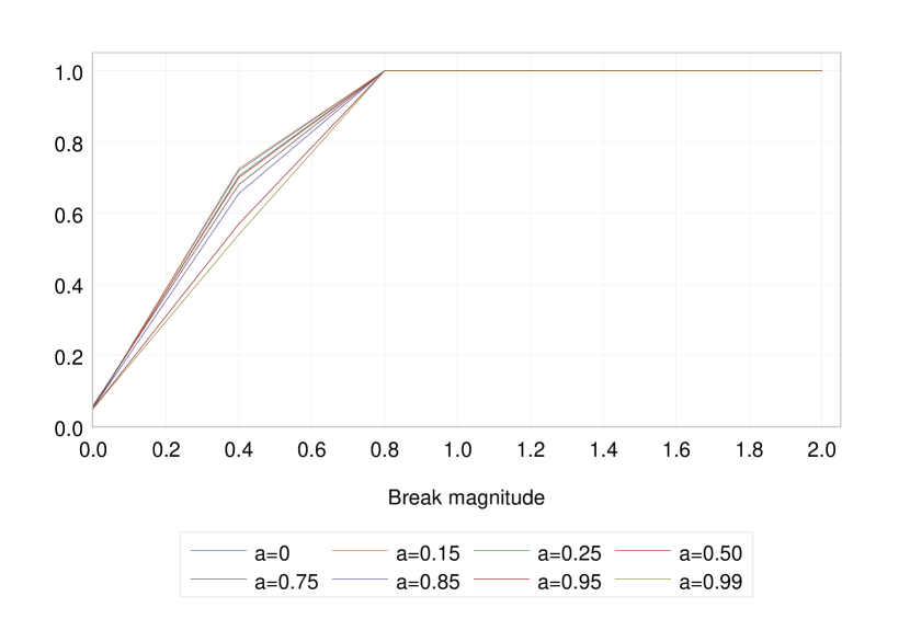
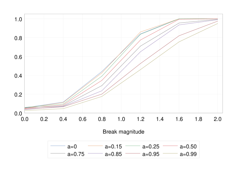
Figure 5.1. Empirical rejection frequencies under a mid-sample break, $N=200$ - i.i.d. data (left panel) and data with serial dependence and measurement error (right panel)

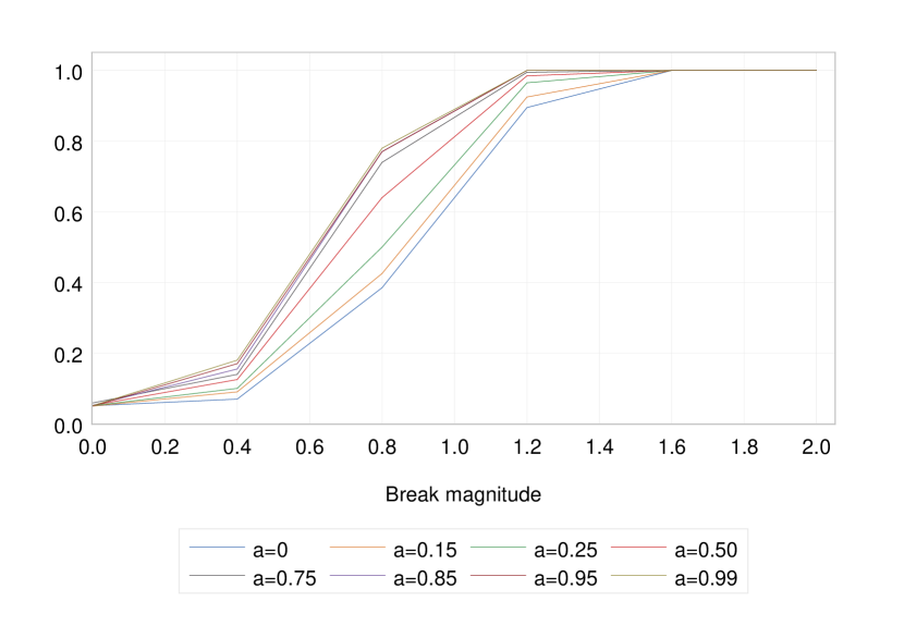
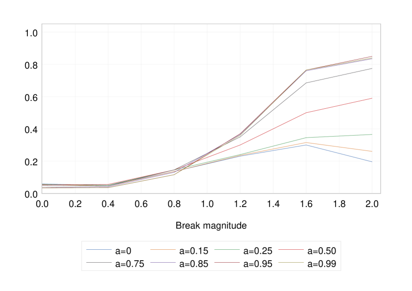
Figure 5.2. Empirical rejection frequencies under an end-of-sample break, $N=200$ - i.i.d. data (left panel) and data with serial dependence and measurement error (right panel)

In a second set of experiments, we explore the performance of our methodology to test for changes in the distribution proposed in Section 4 via a small Monte Carlo exercise. We generate the one-dimensional functional data ${Y_{\ell}}(t)$ using (5.1) with no measurement error, viz. ${Y_{\ell}}(t)=\mu_{\ell}(t)+\epsilon_{\ell}(t)$ with $\epsilon_{\ell}(t)$

(5.4) $$\epsilon_{\ell}(t)=\sum_{m=1}^{M}\lambda_{m}^{1/2}\mathcal{Z}_{m,\ell}\phi_{m}(t).$$

We project $Y_{\ell}(t)$ onto its first Principal Component - that is, we use $d=1$ in (4.4). We do this merely for computational simplicity; when computing the eigenvalues of the long-run variance matrix associated with $X_{\ell}(t)$, we use the algorithm in Section 3.2 in Happ and Greven (2018), based on the multivariate KL expansion. In Table 5.2, we report the empirical rejection frequencies under the null, showing that our methodology has excellent size control for $N\geq 100$; when $N=50$, tests appear to be mildly oversized.

Table 5.2. Empirical rejection frequencies under the null of no changepoint in distribution - i.i.d. data

$N$	$\alpha$		$0.00$	$0.10$	$0.25$	$0.50$	$0.75$	$0.85$	$0.95$	$0.99$
$50$			$0.067$	$0.069$	$0.069$	$0.069$	$0.072$	$0.072$	$0.077$	$0.076$
$100$			$0.058$	$0.058$	$0.057$	$0.056$	$0.057$	$0.056$	$0.059$	$0.061$
$150$			$0.053$	$0.051$	$0.050$	$0.050$	$0.051$	$0.047$	$0.049$	$0.048$
$200$			$0.057$	$0.057$	$0.054$	$0.053$	$0.052$	$0.056$	$0.060$	$0.057$

• The table contains the empirical rejection frequencies under the null of no changepoint. Data are generated according to (5.4) with specifications as in the main text, for tests at a $5\%$ nominal level.

We separately consider the following alternative hypotheses:

(5.5) $$\mu_{\ell}(t)=\mathcal{\delta}(t)I\left(k^{\ast}\leq\ell\leq N\right),$$

with $\left\|\mathcal{\delta}\right\|=1$, to consider changes in the mean function;

(5.6) $$\sigma_{\mathcal{Z}}=\sigma_{\mathcal{Z},\ell}=I\left(1\leq\ell<k^{\ast}\right)+2I\left(k^{\ast}\leq\ell\leq N\right),$$

with $\mu_{\ell}(t)=0$ for all $1\leq\ell\leq N$, to consider a change in the (unconditional) variance which is helpful to understand whether our methodology can detect heteroskedasticity; and lastly

(5.7) $$\epsilon_{\ell}(t)=\left(\sum_{m=1}^{M}\lambda_{m}^{1/2}\mathcal{Z}_{m,\ell}\phi_{m}(t)\right)I\left(1\leq\ell<k^{\ast}\right)+\left(\sum_{m=1}^{M}\lambda_{m}^{1/2}t_{m,\ell}^{\left(3\right)}\phi_{m}(t)\right)I\left(k^{\ast}\leq\ell\leq N\right),$$

where $t_{m,\ell}^{\left(3\right)}$ are i.i.d. random variables, independent across $m$ and $\ell$, with a Student’s t distribution with $3$ degrees of freedom, and $\mu_{\ell}(t)=0$ for all $1\leq\ell\leq N$, as a more general alternative where the data, after a period of “normal” fluctuations, exhibit heavy tails. Results in Table 5.3 show that our tests - even when using $d=1$ - have excellent power under all cases in the presence of a mid-sample break, which is also estimated correctly. Hence, the test developed in Section 4 can be used to detect shifts in the mean, in the variance, or in the tails - of course, the test is an omnibus test, and therefore it is non-constructive in that, upon rejecting the null, it does not indicate a specific alternative. In the case of end-of-sample breaks, Table 5.4 shows that the test is sensitive, as expected, to the choice of $\alpha$, and that as $\alpha$ approaches $1$ the power increases, as does the accuracy in estimating the changepoint. The test performs very well, even for small sample sizes ($N=100$) in the presence of changes in the mean and in the tails (i.e., under (5.5) and (5.7) respectively), whereas its performance is less good in the presence of shifts in the variance (i.e., under (5.6)) although it picks up as both $\alpha$ and $N$ increase.

Table 5.3. Empirical rejection frequencies in the presence of a mid-sample changepoint in distribution

Empirical rejection frequencies under (5.5)
$N$	$\alpha$		$0.00$	$0.10$	$0.25$	$0.50$	$0.75$	$0.85$	$0.95$	$0.99$
$100$			$\underset{\left(50\right)}{0.875}$	$\underset{\left(50\right)}{0.885}$	$\underset{\left(50\right)}{0.885}$	$\underset{\left(50\right)}{0.875}$	$\underset{\left(50\right)}{0.870}$	$\underset{\left(50\right)}{0.865}$	$\underset{\left(50\right)}{0.855}$	$\underset{\left(50\right)}{0.850}$
$200$			$\underset{\left(100\right)}{1.000}$	$\underset{\left(100\right)}{1.000}$	$\underset{\left(100\right)}{1.000}$	$\underset{\left(100\right)}{1.000}$	$\underset{\left(100\right)}{1.000}$	$\underset{\left(100\right)}{1.000}$	$\underset{\left(100\right)}{1.000}$	$\underset{\left(100\right)}{1.000}$
Empirical rejection frequencies under (5.6)
$N$	$\alpha$		$0.00$	$0.10$	$0.25$	$0.50$	$0.75$	$0.85$	$0.95$	$0.99$
$100$			$\underset{\left(51\right)}{0.925}$	$\underset{\left(51\right)}{0.925}$	$\underset{\left(51\right)}{0.925}$	$\underset{\left(51\right)}{0.905}$	$\underset{\left(51\right)}{0.850}$	$\underset{\left(51\right)}{0.830}$	$\underset{\left(51\right)}{0.790}$	$\underset{\left(51\right)}{0.765}$
$200$			$\underset{\left(101\right)}{1.000}$	$\underset{\left(101\right)}{1.000}$	$\underset{\left(101\right)}{1.000}$	$\underset{\left(101\right)}{1.000}$	$\underset{\left(101\right)}{1.000}$	$\underset{\left(101\right)}{1.000}$	$\underset{\left(101\right)}{1.000}$	$\underset{\left(101\right)}{1.000}$
Empirical rejection frequencies under (5.7)
$N$	$\alpha$		$0.00$	$0.10$	$0.25$	$0.50$	$0.75$	$0.85$	$0.95$	$0.99$
$100$			$\underset{\left(51\right)}{0.945}$	$\underset{\left(51\right)}{0.945}$	$\underset{\left(51\right)}{0.945}$	$\underset{\left(51\right)}{0.950}$	$\underset{\left(51\right)}{0.945}$	$\underset{\left(51\right)}{0.945}$	$\underset{\left(51\right)}{0.930}$	$\underset{\left(51\right)}{0.915}$
$200$			$\underset{\left(100\right)}{1.000}$	$\underset{\left(100.5\right)}{1.000}$	$\underset{\left(100.5\right)}{1.000}$	$\underset{\left(101\right)}{1.000}$	$\underset{\left(101\right)}{1.000}$	$\underset{\left(101\right)}{1.000}$	$\underset{\left(101\right)}{1.000}$	$\underset{\left(101\right)}{1.000}$

• The table contains the empirical rejection frequencies under a changepoint occurring at $k^{\ast}=N/2$; the numbers in round brackets are the median estimated break dates. Data are generated according to (5.4) with specifications as in the main text, for tests at a $5\%$ nominal level, under the alternative hypotheses in (5.5)-(5.7).

Table 5.4. Empirical rejection frequencies in the presence of an end-of-sample changepoint in distribution

Empirical rejection frequencies under (5.5)
$N$	$\alpha$		$0.00$	$0.10$	$0.25$	$0.50$	$0.75$	$0.85$	$0.95$	$0.99$
$100$			$\underset{\left(71\right)}{0.200}$	$\underset{\left(71\right)}{0.210}$	$\underset{\left(71.5\right)}{0.220}$	$\underset{\left(81\right)}{0.265}$	$\underset{\left(86.5\right)}{0.340}$	$\underset{\left(88\right)}{0.360}$	$\underset{\left(89.5\right)}{0.380}$	$\underset{\left(90\right)}{0.380}$
$200$			$\underset{\left(157\right)}{0.485}$	$\underset{\left(160\right)}{0.525}$	$\underset{\left(164\right)}{0.555}$	$\underset{\left(172.5\right)}{0.620}$	$\underset{\left(177\right)}{0.695}$	$\underset{\left(179\right)}{0.715}$	$\underset{\left(179\right)}{0.725}$	$\underset{\left(179\right)}{0.735}$
Empirical rejection frequencies under (5.6)
$N$	$\alpha$		$0.00$	$0.10$	$0.25$	$0.50$	$0.75$	$0.85$	$0.95$	$0.99$
$100$			$\underset{\left(63\right)}{0.145}$	$\underset{\left(79\right)}{0.165}$	$\underset{\left(83.5\right)}{0.200}$	$\underset{\left(89\right)}{0.260}$	$\underset{\left(90\right)}{0.340}$	$\underset{\left(90\right)}{0.370}$	$\underset{\left(91\right)}{0.400}$	$\underset{\left(91\right)}{0.410}$
$200$			$\underset{\left(156.5\right)}{0.300}$	$\underset{\left(162.5\right)}{0.320}$	$\underset{\left(171\right)}{0.370}$	$\underset{\left(179\right)}{0.455}$	$\underset{\left(180\right)}{0.545}$	$\underset{\left(180\right)}{0.560}$	$\underset{\left(180\right)}{0.590}$	$\underset{\left(180\right)}{0.595}$
Empirical rejection frequencies under (5.7)
$N$	$\alpha$		$0.00$	$0.10$	$0.25$	$0.50$	$0.75$	$0.85$	$0.95$	$0.99$
$100$			$\underset{\left(86\right)}{0.320}$	$\underset{\left(88\right)}{0.345}$	$\underset{\left(90\right)}{0.385}$	$\underset{\left(90\right)}{0.460}$	$\underset{\left(90\right)}{0.575}$	$\underset{\left(91\right)}{0.610}$	$\underset{\left(91\right)}{0.650}$	$\underset{\left(91\right)}{0.660}$
$200$			$\underset{\left(173\right)}{0.505}$	$\underset{\left(178\right)}{0.540}$	$\underset{\left(179\right)}{0.630}$	$\underset{\left(180\right)}{0.750}$	$\underset{\left(180\right)}{0.835}$	$\underset{\left(180\right)}{0.855}$	$\underset{\left(181\right)}{0.860}$	$\underset{\left(181\right)}{0.860}$

• The table contains the empirical rejection frequencies under a changepoint occurring at $k^{\ast}=0.9N$; the numbers in round brackets are the median estimated break dates. Data are generated according to (5.4) with specifications as in the main text, for tests at a $5\%$ nominal level, under the alternative hypotheses in (5.5)-(5.7).

6. Changepoint detection in high-frequency financial data

We apply our tests for changepoint detection in the mean and in the distribution of intraday return patterns (on a month-on-month basis) in high-frequency trading of the S&P 500 index. High-frequency trading data lend themselves to being studied through the lenses of FDA, as they typically contain a huge amount of data for which a parsimonious representation is necessary; furthermore prices change continuously on a daily basis, and therefore daily prices are genuinely functional objects, whose sampling points are the observed prices recorded over several points in time each day. Examples of applications of FDA to high frequency financial data include e.g. Gençay et al. (2001), and Müller et al. (2011); Kokoszka and Zhang (2012) consider an alternative definition of return (know as cumulative intraday returns, or CIDRs) which seems to be particularly suited for predictions using FDA.

Returns are calculated from closing prices that are recorded at equispaced 5-min intervals between $00:00$ and $23:55$ each day, corresponding to a sampling frequency $S=276$. We have used the period spanning from January 3rd, $2022$, until September 3rd, $2023$. In order to balance the sample and ensure that there are $S=276$ sampling points each day, we have removed $21$ trading daily curves in which some data were missing, for a total of $414$ functional datapoints. Denoting prices at day $i$ as $P_{i}\left(t\right)$, we construct month-on-month log returns as $Y_{i}\left(t\right)=\ln P_{i}\left(t\right)-\ln P_{i-21}\left(t\right)$, having used $21$ lags as the average amount of trading days in a month; hence, the resulting sample size is $N=393$, effectively starting from February 3rd, $2022$. We have implemented our test using the guidelines and specifications suggested in Section 5. In particular, when using the KL expansion, we employ a number of bases $\widehat{M}$, chosen so that the first $\widehat{M}$ eigenvalues of the estimated long-run variance explain $95\%$ of the total variability; we note that, in unreported experiments, altering this specification did not change any of the final results. Contrary to Section 5, we use an estimate of the covariance kernel $\mathbf{D}\left(t,s\right)$ computed using the estimator of the covariance functions (3.22) with pre- and post-break demeaning; we note that we tried to use $\widehat{\mathbf{D}}_{N}(t,s)$ defined in (3.21) - that is, without demeaning before and after the candidate breakdate - but results do not change in any way. Upon inspection, this is due to the fact that, across all exercises, the bandwidth is selected as at most $h=1$; this, in turn, suggests that the data have only little serial dependence. We tried to assess the sensitivity of our results by varying $h$, but virtually no changes were noted. Finally, results are reported at a nominal level of $5\%$; however, we have also carried out - by way of sensitivity analysis - detection at $1\%$ and $10\%$ levels, and results are discussed in the notes of our tables.

We begin by applying our test for a changepoint in the mean. In Table 6.1, we report results for $\alpha=0.5$, but we also tried $\alpha=0$ and $\alpha=0.99$, obtaining exactly the same outcome: there is only one break, located at October 20th, $2022$, whose estimate appears to be remarkably robust (note also the discrepancy between the daily averages). Whilst it is difficult to associate a particular event to that date, in general the common wisdom among financial analysts is that S&P 500 index started recovering, after a turbulent year and after hitting its low in October $2022$, around the second half of that month. No further breaks in the mean function were found.

Table 6.1. Changepoint in the mean in intraday, month-on-month return curves - S&P 500, January 3rd, 2022 - September 3rd, 2023

Changepoint detection in the mean
	Iteration		Segment		Outcome		Estimated date		Notes
	$1$		Jan 3rd, 2022 – Sep 3rd, 2023		Reject		Oct 20th, 2022		significant also at $1\%$
									break found also using $\alpha=0,$ $0.99$, at the same date
									daily average = $0.00268$
	$2$		Oct 20th, 2022 – Sep 3rd, 2023		Not reject				no break found even at $10\%$
									daily average = $-0.02493$
	$3$		Jan 3rd, 2022 – Oct 19th, 2022		Not reject				no break found even at $10\%$
									daily average = $0.01631$

• Daily averages are computed as averages within each regime, and across sampling points.

It is well known (see e.g. Kim and White, 2004) that the behaviour of financial markets is characterised by not being adequately described by the Gaussian distribution; hence, it is important to check if there are changes not merely in the mean (or in the variance), but in the whole distribution. Thus, after finding the presence of a break in the mean, we demean the data in each of the two segments around October 20th, $2022$, and carry out the test for distributional changes, on the demeaned data, discussed in Section 4. We use exactly the same specifications as in Section 5, using only one principal component (i.e. $d=1$) in the construction of $X_{i}(t)$ in (4.4). Tests are carried out at a nominal level of $5\%$ by default (we also tried $1\%$ and $10\%$, see the notes to Table B.1); when using binary segmentation, we use, as threshold, $\tau_{N}=c_{a}\sqrt{\ln N}$, where $a$ is the nominal level of the test; results are generally robust to this (we tried $\tau_{N}=c_{a}\ln\ln N$, and $\tau_{N}=c_{a}{\ln N}$, and no changes were noted). We report our findings using weights $\alpha=0$, $0.5$ and $0.99$; we used binary segmentation, so the case $\alpha=0$ is not reliable per se, as it may lead to overestimation of the number of regimes, but we use it as a benchmark for the other two sets of results.

Table 6.2. Changepoint in the distribution in intraday, month-on-month return curves - S&P 500, January 3rd, 2022 - September 3rd, 2023

Changepoint detection using $\alpha=0.50$
	Iteration		Segment		Outcome		Estimated date		Notes
	$1$		Jan 3rd, 2022 – Sep 3rd, 2023		Reject		Oct 20th, 2022		significant also at $1\%$
									break found also using $\alpha=0,$ $0.99$, at the same date
	$2$		Oct 20th, 2022 – Sep 3rd, 2023		Not reject				no break found even at $10\%$, or with $\alpha=0,$ $0.99$
									$\begin{array}[]{c}\widehat{\sigma}_{N}^{2}=0.002\\ sk=0.950\\ ku=2.008\end{array}$
	$3$		Jan 3rd, 2022 – Oct 19th, 2022		Reject		Aug 30th, 2022		significant at $5\%$
									break found also using $\alpha=0,$ at the same date
									break found also using $\alpha=0.99,$ Sep 12th, 2022
	$4$		Aug 30th, 2022 – Oct 19th, 2022		Not reject				no break found even at $10\%$, or with $\alpha=0,$ $0.99$
									$\begin{array}[]{c}\widehat{\sigma}_{N}^{2}=0.006\\ sk=-1.234\\ ku=1.635\end{array}$
	$5$		Jan 3rd, 2022 – Aug 29th, 2022		Reject		Jul 13th, 2022		significant at $5\%$
									break found also using $\alpha=0.99$, at the same date
									break found also using $\alpha=0$, at Jul 14th, 2022
	$6$		Jul 13th, 2022 – Aug 29th, 2022		Not reject				no break found even at $10\%$, or with $\alpha=0,$ $0.99$
									$\begin{array}[]{c}\widehat{\sigma}_{N}^{2}=0.005\\ sk=1.233\\ ku=1.656\end{array}$
	$7$		Jan 3rd, 2022 – Jul 12th, 2022		Reject		Apr 21st, 2022		significant at $5\%$
									break found also using $\alpha=0,0.99$, at the same date
	$8$		Jan 3rd, 2022 – Apr 20th, 2022		Reject		Mar 20th, 2022		significant at $5\%$
									break found also using $\alpha=0,0.99$, at the same date
	$9$		Jan 3rd, 2022 – Mar 19th, 2022		Not reject				no break found even at $10\%$, or with $\alpha=0,$ $0.99$
									$\begin{array}[]{c}\widehat{\sigma}_{N}^{2}=0.002\\ sk=-1.269\\ ku=1.734\end{array}$
	$10$		Mar 20th, 2022 – Apr 20th, 2022		Not reject				no break found even at $10\%$, or with $\alpha=0,$ $0.99$
									$\begin{array}[]{c}\widehat{\sigma}_{N}^{2}=0.003\\ sk=1.247\\ ku=1.645\end{array}$
	$11$		Apr 21st, 2022 – Jul 12th, 2022		Not reject				no break found even at $10\%$, or with $\alpha=0,$ $0.99$
									$\begin{array}[]{c}\widehat{\sigma}_{N}^{2}=0.005\\ sk=-1.291\\ ku=1.807\end{array}$

• We have used the estimator of the variance $\widehat{\sigma}_{N}^{2}$ defined in (3.25). As far as the other descriptive statistics are concerned, “$sk$” and “$ku$” represent overall measures of skewness and kurtosis respectively, computed within each regime, and across sampling points (see equations (C.1) and (C.2) in the Supplement).

The results in Table B.1 show a much richer picture that changes in the mean alone. Interestingly, the same changepoints are found across all values of $\alpha$, including $\alpha=0$; the only difference is in the date of the break estimated between July and October $2022$, which appears to be estimated $8$ trading days later when using larger values of $\alpha$. Otherwise, results are exactly the same; indeed, we also experimented with other values, but results were the same even in those cases. The same robustness was found when altering other specifications of the procedure, e.g. the estimation the covariance kernel or of the number of terms $\widehat{M}$ in the KL expansion. The estimated breakdates are, at least in some cases, highly suggestive; interestingly, in all cases, a change in regime corresponds to a change in the sign of our measure of skewness, which confirms the stylised fact that skewness is time-varying (Alles and Kling, 1994; Bekaert et al., 1998). The first break, recorded at March 20th, $2022$, corresponds to a peak in the S&P 500, after which the market entered a bear phase to stay below that peak until July $2023$; after removing the first 21 observations, our month-on-month return series starts effectively in February, so that the first regime - characterised by a strongly negative measure of skewness - reflects the uncertainty due to the war in Ukraine and its impact on the global economy. The second regime, between March 20th and April 20th, is characterised by a positive skewness, possibly indicating that the market - after the stalling of the Russian offensive - was expecting an upward price movement. This did not materialise, and in April $2022$ the market experienced a strong correction, partly also due to inflation expectation and underperformance of high-tech firms. After April 20th the market entered a bear phase, chracterised by negative skewness, until a turning point was reached on July13th, $2022$ on account of the FED ending (temporarily) its rate hiking. A correction occurred after August 30th, $2022$, with a slump that lasted until approximately the second half of October (the changepoint was recorded on October 20th, $2022$). From thereon, the market started a rebound which lasted for the remainder of our sample period; during this long horizon, the market was again characterised by positive skewness.

7. Discussion and conclusions

In this paper, we propose a family of weighted statistics to detect changepoints possibly dependent, multivariate functional data. Although we focus our exposition on the well-studied case of changes in the mean, our tests can be applied to much more general changepoint problems, such as detecting changes in the whole distribution. We base our test statistics on the notion of energy distance, a recently proposed measure of proximity between distributions; we use a version of the (empirical) energy distance which is particularly suited to determining the equality of the first moment of random variables, showing that, under the null of no breaks, this is related to the familiar CUSUM process. Our statistics can be applied under very general forms of (weak) serial dependence, thus being suitable for the analysis of several datasets, including meteorological, financial and economic time series. By using a set of weights which place more emphasis on observations occurring close to the sample endpoints, we are able to detect changepoints occurring very close to the beginning/end of the sample. Also, our approach is sufficiently flexible to allow for generalisations to e.g. testing for changepoints in the (marginal) distributions of a sequence. In particular, our approach is based on checking whether expectations of functions of our data remain constant over time; consequently, we can use all the technology available in the literature, such as e.g. binary segmentation in order to detect (and estimate the number and location of) multiple changepoints. An important feature of our procedures is its computational simplicity: critical values can be derived with arbitrary precision, and this requires only the eigenvalues of the covariance operator of the data, which can be quickly computed via any available statistical package. Our simulations show that our statistics have excellent finite sample performance even for small samples, thus making their use possible in virtually all contexts involving FDA.

This work leads to several possible future directions, including extensions to energy distances for functional data beyond the case $\eta=2$, and more broadly further exploration of generalized energy distances. The use of the characteristic function in Section 4 can be viewed as a finite-dimensional approximation of the characteristic functional; an interesting direction would be to more deeply explore finite-dimensional approximations of the characteristic functional and similar transformations in the context of functional time series.

A. Further Monte Carlo evidence and guidelines

A.1. Empirical rejection frequencies under the null: further results

We complement the results in Table 5.1 by considering the cases of i.i.d. data with measurement error, and the case of serially dependent data without measurement error.

Table A.1. Empirical rejection frequencies under the null of no changepoint

			serial dependence, no measurement error										i.i.d. case with measurement error
$N$	$\alpha$		$0.00$	$0.10$	$0.25$	$0.50$	$0.75$	$0.85$	$0.95$	$0.99$			$0.00$	$0.10$	$0.25$	$0.50$	$0.75$	$0.85$	$0.95$	$0.99$
$50$			$0.020$	$0.019$	$0.016$	$0.013$	$0.013$	$0.016$	$0.014$	$0.014$			$0.052$	$0.057$	$0.049$	$0.053$	$0.046$	$0.053$	$0.052$	$0.059$
$100$			$0.049$	$0.045$	$0.043$	$0.036$	$0.033$	$0.027$	$0.022$	$0.018$			$0.045$	$0.051$	$0.052$	$0.048$	$0.056$	$0.044$	$0.054$	$0.047$
$150$			$0.039$	$0.038$	$0.036$	$0.032$	$0.026$	$0.027$	$0.023$	$0.019$			$0.044$	$0.052$	$0.051$	$0.050$	$0.054$	$0.045$	$0.066$	$0.049$
$200$			$0.058$	$0.055$	$0.055$	$0.052$	$0.047$	$0.035$	$0.034$	$0.033$			$0.055$	$0.052$	$0.052$	$0.050$	$0.056$	$0.050$	$0.056$	$0.059$

• The table contains the empirical rejection frequencies under the null of no changepoint, using $M=40$ orthonormal bases in (5.1), for tests at a $5\%$ nominal level. The specifications of (5.1) are described in the main text.

A.2. Empirical rejection frequencies under the alternative: further results

We begin by reporting the power against one changepoint, with the same design as in equation (5.3) using $N=100$. As can be seen in Figures A.1 and A.2, the results are similar, although the test is less powerful compared to the results in Figures 5.1 and 5.2, which is expected due to the smaller value of $N$. In particular, in the presence of an end-of-sample break, power is ensured only for large values of $\alpha$.

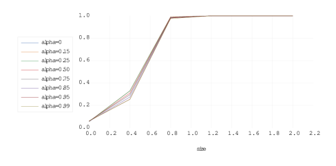
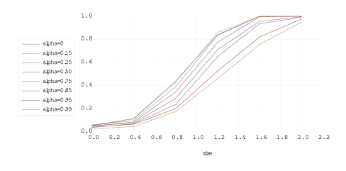
Figure A.1. Empirical rejection frequencies under a mid-sample break with i.i.d. data and data with serial dependence and measurement error

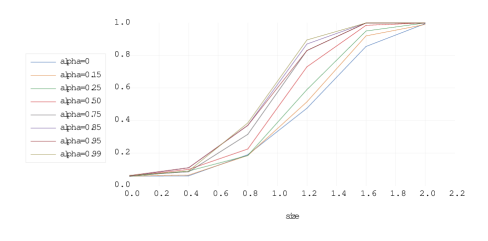
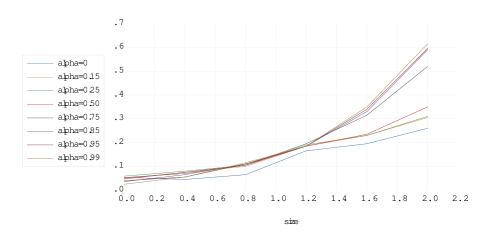
Figure A.2. Empirical rejection frequencies under a mid-sample break with i.i.d. data and data with serial dependence and measurement error

We now report the median values of the estimated breakdate $k^{\ast}$, in the case of a single changepoint (when this is detected), under the same set-up as in Section 5 - see equation (5.3) in particular. Results in Tables A.2-A.5 should be read in conjunction with Figures A.1-A.2 and 5.1-5.2, and broadly confirm the theory spelled out in Theorem 3.3. In the case of mid-sample breaks, the estimator of $k^{\ast}$ is usually very good when a changepoint is detected (Tables A.2-A.3), even for small break sizes like $\left\|\mathcal{\delta}\right\|=0.4$; this is true across all values of $\alpha$, although, in the case of small breaks ($\left\|\mathcal{\delta}\right\|=0.4$), the performance of $\widehat{k}$ when $\alpha$ gets closer to $1$ seems to worsen. Conversely, when breaks occur close to the end of the sample ($k^{\ast}=0.9N$), results in Table A.4 and A.5 differ dramatically across $\alpha$: as expected, when $\alpha$ increases, $\widehat{k}$ performs better, and it performs very well when $\left\|\mathcal{\delta}\right\|\geq 0.8$ (and even more so when $N=200$). Interestingly, in this case $\widehat{k}$ appears to have a downward bias, which vanishes as $N\left\|\mathcal{\delta}\right\|$ increases.

Table A.2. Median estimated changepoints under a mid-sample changepoint, i.i.d. data, no measurement error

			$N=100$, $k^{\ast}=50$										$N=200$, $k^{\ast}=100$
	$\alpha$			$0.00$	$0.10$	$0.25$	$0.50$	$0.75$	$0.85$	$0.95$	$0.99$			$0.00$	$0.10$	$0.25$	$0.50$	$0.75$	$0.85$	$0.95$	$0.99$
$\left\|\mathcal{\delta}\right\|$
$0.40$				$50$	$50$	$50$	$50$	$49$	$50$	$49$	$50$			$100$	$101$	$101$	$101$	$101$	$100$	$100$	$100$
$0.80$				$50$	$50$	$50$	$50$	$50$	$50$	$50$	$50$			$100$	$100$	$100$	$100$	$100$	$100$	$100$	$100$
$1.20$				$50$	$50$	$50$	$50$	$50$	$50$	$50$	$50$			$100$	$100$	$100$	$100$	$100$	$100$	$100$	$100$
$1.60$				$50$	$50$	$50$	$50$	$50$	$50$	$50$	$50$			$100$	$100$	$100$	$100$	$100$	$100$	$100$	$100$
$2.00$				$50$	$50$	$50$	$50$	$50$	$50$	$50$	$50$			$100$	$100$	$100$	$100$	$100$	$100$	$100$	$100$

• The table contains the median estimated changepoint in the presence of a mid-sample break, for different values of $\alpha$, $\left\|\mathcal{\delta}\right\|$, and sample sizes $N$, with $\rho=0$. All figures are based on $200$ replications.

Table A.3. Median estimated changepoints under a mid-sample changepoint, serially dependent data with measurement error

			$N=100$, $k^{\ast}=50$										$N=200$, $k^{\ast}=100$
	$\alpha$			$0.00$	$0.10$	$0.25$	$0.50$	$0.75$	$0.85$	$0.95$	$0.99$			$0.00$	$0.10$	$0.25$	$0.50$	$0.75$	$0.85$	$0.95$	$0.99$
$\left\|\mathcal{\delta}\right\|$
$0.40$				$49$	$49.5$	$49.5$	$54$	$58.5$	$58.5$	$75$	$88.5$			$97$	$104$	$107$	$107$	$113$	$111$	$114.5$	$119$
$0.80$				$50$	$50$	$51$	$51$	$52$	$52$	$52$	$51$			$99$	$100$	$100$	$101$	$101$	$100$	$100$	$100$
$1.20$				$50$	$50$	$50$	$50$	$50$	$50$	$50$	$50$			$100$	$100$	$100$	$100$	$100$	$100$	$100$	$100$
$1.60$				$50$	$50$	$50$	$50$	$50$	$50$	$50$	$50$			$100$	$100$	$100$	$100$	$100$	$100$	$100$	$100$
$2.00$				$50$	$50$	$50$	$50$	$50$	$50$	$50$	$50$			$100$	$100$	$100$	$100$	$100$	$100$	$100$	$100$

• The table contains the median estimated changepoint in the presence of a mid-sample break, for different values of $\alpha$, $\left\|\mathcal{\delta}\right\|$, and sample sizes $N$, with $\rho=0.5$. All figures are based on $200$ replications.

Table A.4. Median estimated changepoints under an end-of-sample changepoint, i.i.d. data, no measurement error

			$N=100$, $k^{\ast}=90$										$N=200$, $k^{\ast}=180$
	$\alpha$			$0.00$	$0.10$	$0.25$	$0.50$	$0.75$	$0.85$	$0.95$	$0.99$			$0.00$	$0.10$	$0.25$	$0.50$	$0.75$	$0.85$	$0.95$	$0.99$
$\left\|\mathcal{\delta}\right\|$
$0.40$				$56$	$57$	$54.5$	$56$	$63$	$81$	$82$	$87.5$			$110.5$	$106.5$	$110.5$	$145$	$166.5$	$175$	$176$	$177$
$0.80$				$57.5$	$61$	$62$	$73$	$85$	$89$	$90$	$90$			$145.5$	$148.5$	$161$	$176$	$179$	$180$	$180$	$180$
$1.20$				$71$	$78$	$82$	$89$	$90$	$90$	$90$	$90$			$161$	$166$	$175$	$179$	$180$	$180$	$180$	$180$
$1.60$				$81$	$84$	$88$	$90$	$90$	$90$	$90$	$90$			$177.5$	$178$	$179$	$179$	$180$	$180$	$180$	$180$
$2.00$				$86$	$87$	$89$	$90$	$90$	$90$	$90$	$90$			$178$	$178$	$179$	$180$	$180$	$180$	$180$	$180$

• The table contains the median estimated changepoint in the presence of a mid-sample break, for different values of $\alpha$, $\left\|\mathcal{\delta}\right\|$, and sample sizes $N$, with $\rho=0.5$ and $\sigma_{v}=0.25$. All figures are based on $200$ replications.

Table A.5. Median estimated changepoints under an end-of-sample changepoint, serially dependent data with measurement error

			$N=100$, $k^{\ast}=90$										$N=200$, $k^{\ast}=180$
	$\alpha$			$0.00$	$0.10$	$0.25$	$0.50$	$0.75$	$0.85$	$0.95$	$0.99$			$0.00$	$0.10$	$0.25$	$0.50$	$0.75$	$0.85$	$0.95$	$0.99$
$\left\|\mathcal{\delta}\right\|$
$0.40$				$58$	$57.5$	$61$	$57.5$	$75$	$75.5$	$75.5$	$82$			$93$	$89$	$105.5$	$118$	$118$	$105.5$	$118$	$118$
$0.80$				$54.5$	$54.5$	$54$	$54$	$61$	$61$	$68$	$81.5$			$94$	$90$	$113.5$	$116.5$	$123$	$142$	$142$	$165$
$1.20$				$53$	$54.5$	$53$	$61$	$76$	$77$	$83$	$87.5$			$103$	$102$	$116$	$131.5$	$163$	$172$	$177$	$178$
$1.60$				$53$	$54$	$53$	$73$	$81$	$87$	$89.5$	$90$			$111$	$111$	$125$	$158$	$178$	$179$	$180$	$180$
$2.00$				$54$	$58.5$	$59$	$76$	$88$	$90$	$90$	$90$			$134$	$143$	$163$	$179$	$180$	$180$	$180$	$180$

• The table contains the median estimated changepoint in the presence of an end-of-sample break, for different values of $\alpha$, $\left\|\mathcal{\delta}\right\|$, and sample sizes $N$, with $\rho=0.5$ and $\sigma_{v}=0.25$. All figures are based on $200$ replications.

A.3. Binary segmentation: pesudocode and Monte Carlo evidence

We begin by reporting some pseudocode for the practical implementation of the algorithm. Let, for short

$$\mathcal{Z}_{\ell,u}^{k}=\left(\frac{k}{N}\left(1-\frac{k}{N}\right)\right)^{-\alpha}V_{N}^{\left(\ell,u\right)}\left(k\right).$$

The pseudocode is in Algorithm 1 below.

Algorithm 1 Binary segmentation for functional data based on the empirical energy function: ENERGYSEG($\ell$, $u$, $\tau_{N}$)

starting index $\ell$; ending index $u$; threshold $\tau_{N}$

if $u-\ell\leq 4$ then

     STOP

else if $u-\ell>4$ then

     Define $k_{0}=\operatorname*{sargmax}_{\ell\leq k\leq u}\mathcal{Z}_{\ell,u}^{k}$, and $\mathcal{Z}=\mathcal{Z}_{\ell,u}^{k_{0}}$

end if

if $\mathcal{Z}>\tau_{N}$ then

     add $k_{0}$ to the set of estimated changepoints.

     run ENERGYSEG($l$, $k_{0}$, $\tau_{N}$) and ENERGYSEG($k_{0}$, $u$, $\tau_{N}$)

else STOP

end if

We now report a small Monte Carlo exercise to assess the performance of the binary segmentation procedure discussed in Section 3.2.3. In particular, we consider the following DGP

$$X_{i}(t)=\sum_{j=1}^{R+1}\mu_{j}\left(t\right)I\left\{k_{j-1}\leq i<k_{j}\right\}+\sum_{\ell=1}^{M}\lambda_{\ell}^{1/2}\mathcal{Z}_{\ell,i}\phi_{\ell}(t)+\nu_{i}\left(t\right),$$

where the random part $\sum_{\ell=1}^{M}\lambda_{\ell}^{1/2}\mathcal{Z}_{\ell,i}\phi_{\ell}(t)+\nu_{i}\left(t\right)$ is generated in the same way as in Section 5, and we consider two mid-sample changepoints (i.e., $R=2$) in the mean function $\mu_{j}(t)$, viz.

(A.1) $$\mu_{j}\left(t\right)=\left\{\begin{array}[]{ll}\mathcal{\delta}_{1}(t)&1\leq i<k_{1}^{\ast}\\ \mathcal{\delta}_{2}(t)&k_{1}^{\ast}\leq i<k_{2}^{\ast}\\ \mathcal{\delta}_{3}(t)&k_{2}^{\ast}\leq i\geq N\end{array}\right.,$$

with $k_{1}^{\ast}=\left\lfloor 0.35N\right\rfloor$ and $k_{2}^{\ast}=\left\lfloor 0.7N\right\rfloor$, and $\delta_{i}(t)\equiv C_{\delta_{i}}$ are constants, $C_{\delta_{1}}=0$, $C_{\delta_{2}}=2$ and $C_{\mathcal{\delta}_{3}}=3$. When using Algorithm 1, we select the threshold

(A.2) $$\tau_{N}=c_{a}\log\log N,$$

where $c_{a}$ is the critical value at nominal level $a=0.05$.

Results in Table A.6 contain measures of location of the estimator of the number of changepoints $\widehat{R}$, and the average values, across simulations, of the estimated breakdates, using $500$ simulations. Results are obtained for $N=200$ and with $\mathcal{Z}_{\ell,i}$ generated as i.i.d. across $1\leq i\leq N$; we consider the presence of measurement errors, setting $\sigma_{\nu}^{2}=0.25$ as in Section 5, but in unreported experiments we noted that having $\sigma_{\nu}^{2}=0$ does not change the results in any significant way.

Table A.6. Measures of location for $\widehat{R}$ and the estimated breakdates

Measures of location for the estimated number of changepoints $\widehat{R}$
		$\alpha$		$0.00$	$0.15$	$0.25$	$0.50$	$0.75$	$0.85$	$0.95$	$0.99$
	mean			$1.994$	$1.998$	$1.988$	$1.984$	$1.986$	$1.990$	$1.964$	$2.000$
	median			$2.000$	$2.000$	$2.000$	$2.000$	$2.000$	$2.000$	$2.000$	$2.000$
	min			$0.000$	$0.000$	$0.000$	$0.000$	$0.000$	$0.000$	$0.000$	$0.000$
	max			$3.000$	$3.000$	$3.000$	$3.000$	$3.000$	$4.000$	$4.000$	$4.000$
Median estimated breakdates
		$\alpha$		$0.00$	$0.15$	$0.25$	$0.50$	$0.75$	$0.85$	$0.95$	$0.99$
	$\widehat{k}_{1}$			$70$	$70$	$70$	$70$	$70$	$70$	$70$	$70$
	$\widehat{k}_{2}$			$140$	$140$	$140$	$140$	$140$	$140$	$140$	$140$

• The table contains various measures of location for $\widehat{R}$ and the median estimated breakdates under the alternative (A.1); data have been generated as i.i.d. with measurement error, with sample size $N=200$.

In addition to investigating the performance of binary segmentation in the presence of shifts in the mean as per (A.2), we also explore its performance in the presence of changes in the distribution. In particular, we consider the “epidemic” alternative in a model with zero mean

$${Y_{\ell}}(t)=\epsilon_{\ell}(t),$$

and

(A.3) $$\epsilon_{\ell}(t)=\left\{\begin{array}[]{ll}\displaystyle\sum_{m=1}^{M}\lambda_{m}^{1/2}\mathcal{Z}_{m,\ell}\phi_{m}(t)&1\leq\ell<k_{1}\\ \displaystyle\sum_{m=1}^{M}\lambda_{m}^{1/2}t_{m,\ell}^{\left(3\right)}\phi_{m}(t)&k_{1}\leq\ell<k_{2}\\ \displaystyle\sum_{m=1}^{M}\lambda_{m}^{1/2}\mathcal{Z}_{m,\ell}\phi_{m}(t)&k_{2}\leq\ell\leq N\end{array}\right.,$$

where, as in (5.7), $t_{m,\ell}^{\left(3\right)}$ are i.i.d. random variables, independent across $m$ and $\ell$, with a Student’s t distribution with $3$ degrees of freedom; all the other specifications are the same as above. We use $N=200$ and, as above, $k_{1}^{\ast}=\left\lfloor 0.35N\right\rfloor$ and $k_{2}^{\ast}=\left\lfloor 0.7N\right\rfloor$. Alternative (A.3) represents a case, relevant in practice, where the data experience a period of turbulence characterised by heavy tails, after which they revert to normal. Results are in Table A.7; we found $\tau_{N}=c_{\alpha}(\ln N)^{1/2}$ to be a better choice in this case, and we suggest this choice of threshold when testing for changes in the distribution.

Table A.7. Measures of location for $\widehat{R}$ and the estimated breakdates - testing for distributional changes

Measures of location for the estimated number of changepoints $\widehat{R}$
		$\alpha$		$0.00$	$0.15$	$0.25$	$0.50$	$0.75$	$0.85$	$0.95$	$0.99$
	mean			$1.995$	$2.100$	$1.860$	$2.050$	$1.840$	$1.815$	$1.600$	$1.335$
	median			$2.000$	$2.000$	$2.000$	$2.000$	$2.000$	$2.000$	$0.000$	$0.000$
	min			$0.000$	$0.000$	$0.000$	$0.000$	$0.000$	$0.000$	$0.000$	$0.000$
	max			$6.000$	$5.000$	$5.000$	$6.000$	$7.000$	$6.000$	$6.000$	$6.000$
Median estimated breakdates
		$\alpha$		$0.00$	$0.15$	$0.25$	$0.50$	$0.75$	$0.85$	$0.95$	$0.99$
	$\widehat{k}_{1}$			$70$	$70$	$70$	$70$	$70$	$70$	$70$	$70$
	$\widehat{k}_{2}$			$139$	$140$	$140$	$140$	$139$	$137$	$138$	$137$

• The table contains various measures of location for $\widehat{R}$ and the median estimated breakdates under the alternative (A.3); data have been generated as i.i.d. with measurement error, with sample size $N=200$.

B. Further empirical evidence

B.1. Further empirical evidence: changepoint analysis of cumulative intraday returns

We complement our findings in Section 6 by applying our tests for changes in the mean and in the distribution to cumulative intraday returns (CIDRs henceforth), whose usefulness is demonstrated in a contribution by Kokoszka and Zhang (2012). We use the same dataset as in Section 6, having removed the same curves consisting of partial trading days. CIDRs are defined as

$$Y_{i}\left(t\right)=\log P_{i}\left(t\right)-\log P_{i}\left(t_{0}\right),$$

where $P_{i}\left(t\right)$ is the daily price evaluated at $t$, and $t_{0}$ is, for each day $1\leq i\leq N$, the start of trading for the day (in our case, midnight). Contrary to the use of month-on-month returns, in this case we can use the whole sample of daily curves consisting of $N=414$ functional datapoints.

Tests have been applied with the same specifications as in Section 6 in the main paper. We did not find any changepoints in the mean, irrespective of the value of $\alpha$. Conversely, applying the test for distributional changes to the demeaned data, several changepoints are found, summarised in Table XXX. In the table, as in the rest of the paper, we have computed the measures of skewness and kurtosis as

(C.1) $$\frac{1}{T}\int_{0}^{T}\frac{\displaystyle{N^{-1}\sum_{i=1}^{N}\left(Y_{i}\left(t\right)-N^{-1}\sum_{i=1}^{N}Y_{i}\left(t\right)\right)^{3}}}{\displaystyle{\left(N^{-1}\sum_{i=1}^{N}\left(Y_{i}\left(t\right)-N^{-1}\sum_{i=1}^{N}Y_{i}\left(t\right)\right)^{2}\right)^{3/2}}}dt,$$

(C.2) $$\frac{1}{T}\int_{0}^{T}\frac{\displaystyle{N^{-1}\sum_{i=1}^{N}\left(Y_{i}\left(t\right)-N^{-1}\sum_{i=1}^{N}Y_{i}\left(t\right)\right)^{4}}}{\displaystyle{\left(N^{-1}\sum_{i=1}^{N}\left(Y_{i}\left(t\right)-N^{-1}\sum_{i=1}^{N}Y_{i}\left(t\right)\right)^{2}\right)^{4/2}}}dt.$$

Table B.1. Changepoint in the distribution in intraday, month-on-month return curves - S&P 500, January 3rd, 2022 - September 3rd, 2023

Changepoint detection using $\alpha=0.50$
	Iteration		Segment		Outcome		Estimated date		Notes
	$1$		Jan 3rd, 2022 – Sep 3rd, 2023		Reject		May 5th, 2022		significant also at $1\%$
									break found also using $\alpha=0$, at the same date, and using $\alpha=0.99$, at Apr 25th, 2022
	$2$		Jan 3rd, 2022 – May 4th, 2022		Reject		Jan 20th, 2022		significant also at $1\%$
									break found also using $\alpha=0,$ at Feb 13th, 2022, and using $\alpha=0.99$, at the same date
	$3$		Jan 3rd, 2022 – Jan 19th, 2022		Not reject				no break found even at $10\%$, or with $\alpha=0,$ $0.99$
									$\begin{array}[]{c}\widehat{\sigma}_{N}^{2}=0.017\\ sk=1.019\\ ku=1.050\end{array}$
	$4$		Jan 20th, 2022 – May 4th, 2022		Not reject				no break found even at $10\%$, or with $\alpha=0,$ $0.99$
									$\begin{array}[]{c}\widehat{\sigma}_{N}^{2}=0.005\\ sk=1.183\\ ku=1.477\end{array}$
	$5$		May 5th, 2022 – Sep 3rd, 2023		Reject		May 17th, 2023		significant also at $1\%$
									break found also using $\alpha=0,$ $0.99$, at the same date
	$6$		May 5th, 2022 – May 18th, 2023		Not reject				no break found even at $10\%$, or with $\alpha=0,$ $0.99$
									$\begin{array}[]{c}\widehat{\sigma}_{N}^{2}=0.003\\ sk=-1.522\\ ku=2.737\end{array}$
	$7$		May 18th, 2023 – Sep 3rd, 2023		Reject		Jun 12th, 2023		significant also at $1\%$
									break found also using $\alpha=0,$ $0.99$, at the same date
	$8$		May 18th, 2023 – Jun 11th, 2023		Not reject				no break found even at $10\%$, or with $\alpha=0,$ $0.99$
									$\begin{array}[]{c}\widehat{\sigma}_{N}^{2}=0.001\\ sk=1.334\\ ku=2.349\end{array}$
	$9$		Jun 11th, 2023 – Sep 3rd, 2023		Not reject				no break found even at $10\%$, or with $\alpha=0,$ $0.99$
									$\begin{array}[]{c}\widehat{\sigma}_{N}^{2}=0.004\\ sk=1.103\\ ku=1.278\end{array}$

• We have used the estimator of the variance $\widehat{\sigma}_{N}^{2}$ defined in (3.25). As far as the other descriptive statistics are concerned, “$sk$” and “$ku$” are computed according to equations (C.1) and (C.2) respectively.

B.2. Further empirical evidence: changepoint analysis of temperature data

In this section, we illustrate our approach using temperature data, where FDA is applied “naturally”; more broadly speaking, recent contributions in the area of climate science show that using time series methods can be beneficial (see Diebold and Rudebusch, 2022; Diebold et al., 2023; and Ditlevsen and Ditlevsen, 2023).

Following Berkes et al. (2009), we use a sample of $N=251$ yearly curves, recorded on a daily basis between $1772$ and $2022$. Each curve contains average daily temperatures (in degrees Celsius) recorded in Central England; apart from removing the data corresponding to February 29th in leap years in order to balance the sample, no further transformation is applied to the data. Our techniques are particularly suited to this dataset for a number of reasons: firstly, we do not need to invert any large-scale matrix, contrary to Horváth et al. (1999), and therefore we can use the daily sampling frequency as opposed to transforming it into monthly averages; secondly, temperature data might exhibit linear or nonlinear serial dependence (see e.g. Bowers and Tung, 2018), which our tests are designed to take into account, unlike those proposed in Berkes et al. (2009); and, finally, our weighted test statistics are also suited to detect changepoints occurring close to the end of the sample, thus allowing to shed light on the presence and extent of changes in average temperatures in recent years. We apply our tests for changepoints in the mean using our tests with $\alpha\in\left\{0,0.5,0.65\right\}$, by way of comparison and robustness check; we note that using different values of $\alpha$ does not alter the main conclusions, although higher values of $\alpha$ seem to estimate the changepoint date later and later. In order to take into account the possible presence of multiple changes, we apply binary segmentation. We have implemented our test using the same specifications as described in Section 6 in the main paper, also carrying out the same robustness checks with no noticeable changes in the results.

Table B.2. Changepoint detection in Central England temperatures, $1772-2022$

Changepoint detection with $\alpha=0.00$
	Iteration		Segment		Outcome		Estimated date		Notes
	$1$		$1772-2022$		Reject		$1919$		significant also at $1\%$
	$2$		$1772-1918$		Reject		$1842$		significant only at $5\%$
	$3$		$1772-1841$		Not reject				no break found even at $10\%$
	$4$		$1842-1918$		Not reject				no break found even at $10\%$
	$5$		$1919-2022$		Reject		$1987$		significant also at $1\%$
	$6$		$1919-1986$		Not reject				no break found even at $10\%$
	$7$		$1987-2022$		Not reject				no break found even at $10\%$
Changepoint detection with $\alpha=0.50$
	$1$		$1772-2022$		Reject		$1919$		significant also at $1\%$
	$2$		$1772-1918$		Reject		$1842$		significant only at $5\%$
	$3$		$1772-1841$		Not reject				no break found even at $10\%$
	$4$		$1842-1918$		Not reject				no break found even at $10\%$
	$5$		$1919-2022$		Reject		$1988$		significant also at $1\%$
	$6$		$1919-1987$		Not reject				no break found even at $10\%$
	$7$		$1988-2022$		Not reject				no break found even at $10\%$
Changepoint detection with $\alpha=0.65$
	$1$		$1772-2022$		Reject		$1932$		significant also at $1\%$
	$2$		$1772-1931$		Reject		$1842$		significant also at $1\%$
	$3$		$1772-1841$		Not reject				no break found even at $10\%$
	$4$		$1842-1931$		Not reject				no break found even at $10\%$
	$5$		$1932-2022$		Reject		$1989$		significant also at $1\%$
	$6$		$1932-1988$		Not reject				no break found even at $10\%$
	$7$		$1989-2022$		Not reject				no break found even at $10\%$

Results are in Table B.2; in Figure B.1, we also report the average temperature functions between each of the estimated changepoints for the various values of $\alpha$. With small and medium values of $\alpha$ (i.e., $\alpha=0$ and $\alpha=0.5$), we identify three changepoints. The first one to be identified (corresponding to the “strongest” break) is estimated to have occurred in $1919$. This result is essentially in agreement with the findings in Berkes et al. (2009) (and also in Horváth et al., 1999), where the first changepoint is found around $1926$. This estimated date corresponds to the so-called Early Twentieth Century Warming (Hegerl et al., 2018), a well-documented phenomenon which partly coincides with the well-known phenomenon of warming of the Arctic (Bengtsson et al., 2004), and which “still defies full explanation” (Brönnimann, 2009, p. 735). Our estimated date is ealier than that of Berkes et al. (2009), which could be ascribed to the estimation error, but also to the “pull” effect, on the data, of the UK heatwave of $1911$. We also estimate a breakdate at $1842$, which could be ascribed to the anthropogenic effect of the Industrial Revolution, and again it is similar to the estimate of $1850$ in Berkes et al. (2009). On the other hand, Berkes et al. (2009) also find one changepoint in $1808$. None of our statistics finds evidence of a changepoint around this date, even at $10\%$ nominal level; on account of the lack of serial correlation, our data could be roughly interpreted as falling into the “i.i.d. with measurement error” category, for which our simulations indicate no undersizement and excellent power even in sample sizes. Finally, we find clear evidence of a changepoint in $1987$ ($1988$ when using $\alpha=0.5$, and $1989$ when using $\alpha=0.65$). This is significant even at $1\%$ nominal level, which corresponds to the beginning of (rapid) global warming - the late $1980$’s date confirms the statement, in the “State of the World 1989” WorldWatch report (Koutaissoff, 1989), that the 90’s would be the “turnaround decade” as far as climate change is concerned. Indeed, Figure B.1 shows very clearly the presence of a pronounced increase in average daily temperatures between the first and the fourth subsamples. When using $\alpha=0.65$, essentially the same results are found, but the first changepoint is estimated at $1932$, i.e. one decade later than the other two changepoint estimates. This can be read in the light of the results in Table A.3, which suggest that, as $\alpha$ increases, the estimated changepoint may be increasingly biased.

Finally, we also considered the possible presence of changes in the distribution of temperature data, applying the test developed in Section 4. To this end, we demeaned the data in each segment, and applied the test in Section 4 using $d=1$. Results are in Table B.3. No changepoints were detected for $\alpha=0$ and $\alpha=0.5$, even at $1\%$ nominal level, suggesting that, if a changepoint is present, this is located towards the sample endpoints; indeed, when using $\alpha=0.65$, the presence of one changepoint emerges even at $10\%$ nominal level, with estimated date $1996$. Comparing descriptive statistics, skewness and kurtosis in the two subperiods seem very similar (in both cases suggesting Gaussianity); conversely, the estimated variances seem to indicate that there is a changepoint in the variability of temperatures between the two subperiods.

Table B.3. Changepoint detection in Central England temperatures, $1772-2022$ - changes in the distribution of demeaned data

Changepoint detection with $\alpha=0.00$ and $\alpha=0.50$
	Iteration		Segment		Outcome		Estimated date		Notes
	$1$		$1772-2022$		Not reject				no break found even at $10\%$
Changepoint detection with $\alpha=0.65$
	$1$		$1772-2022$		Reject		$1996$		significant also at $1\%$
	$2$		$1772-1995$		Not reject				no break found even at $10\%$
									$\begin{array}[]{c}\widehat{\sigma}_{N}^{2}=7.42\\ sk=-0.105\\ ku=3.066\end{array}$
	$3$		$1996-2022$		Not reject				no break found even at $10\%$
									$\begin{array}[]{c}\widehat{\sigma}_{N}^{2}=6.73\\ sk=0.166\\ ku=3.092\end{array}$

• We have used the estimator of the variance $\widehat{\sigma}_{N}^{2}$ defined in (3.25). As far as the other descriptive statistics are concerned, “$sk$” and “$ku$” represent overall measures of skewness and kurtosis respectively.

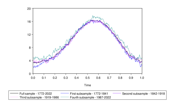
Figure B.1. Average daily temperatures in Central England

Descriptive statistics for the whole sample, and for the segments identified when using $\alpha=0$, are in Table B.4. Results using other values of $\alpha$ (and, therefore, other estimated changepoints) are available upon request.

Table B.4. Descriptive statistics for Central England temperature data: full sample and individual segments

Descriptive statistics - overall period $1772-2022$

Average daily

Average low

Average high

Record low

Record high

First quartile

Median

Third quartile

$9.40$ ${}^{\circ}C$

$-3.62$ ${}^{\circ}C$

$20.99$ ${}^{\circ}C$

$\underset{\left(20/01/1838\right)}{-11.90^{\circ}C}$

$\underset{\left(19/07/2022\right)}{28.10^{\circ}C}$

$5.32$ ${}^{\circ}C$

$9.34$ ${}^{\circ}C$

$13.79$ ${}^{\circ}C$

Descriptive statistics - subperiods

Descriptive statistics - subperiod $1772-1841$

Average daily

Average low

Average high

Record low

Record high

First quartile

Median

Third quartile

$9.12$ ${}^{\circ}C$

$-4.70$ ${}^{\circ}C$

$20.71$ ${}^{\circ}C$

$-11.90$ ${}^{\circ}C$

$24.50$ ${}^{\circ}C$

$4.87$ ${}^{\circ}C$

$9.14$ ${}^{\circ}C$

$13.79$ ${}^{\circ}C$

Descriptive statistics - subperiod $1842-1918$

Average daily

Average low

Average high

Record low

Record high

First quartile

Median

Third quartile

$9.18$ ${}^{\circ}C$

$-3.65$ ${}^{\circ}C$

$20.60$ ${}^{\circ}C$

$-9.00$ ${}^{\circ}C$

$24.00$ ${}^{\circ}C$

$5.16$ ${}^{\circ}C$

$9.10$ ${}^{\circ}C$

$13.51$ ${}^{\circ}C$

Descriptive statistics - subperiod $1919-1986$

Average daily

Average low

Average high

Record low

Record high

First quartile

Median

Third quartile

$9.48$ ${}^{\circ}C$

$-3.28$ ${}^{\circ}C$

$21.02$ ${}^{\circ}C$

$-8.70$ ${}^{\circ}C$

$25.10$ ${}^{\circ}C$

$5.45$ ${}^{\circ}C$

$9.44$ ${}^{\circ}C$

$13.79$ ${}^{\circ}C$

Descriptive statistics - subperiod $1987-2023$

Average daily

Average low

Average high

Record low

Record high

First quartile

Median

Third quartile

$10.22$ ${}^{\circ}C$

$-2.11$ ${}^{\circ}C$

$22.28$ ${}^{\circ}C$

$-7.70$ ${}^{\circ}C$

$28.10$ ${}^{\circ}C$

$6.29$ ${}^{\circ}C$

$10.08$ ${}^{\circ}C$

$14.36$ ${}^{\circ}C$

• The table contains various measures of location - for the full sample and each subsample - for the Central England temperature data.

C. Preliminary lemmas

Henceforth, unless stated otherwise, we carry out our proofs for the case $r=d=1$, for simplicity and without loss of generality. We use the following notation: $\left\lceil\cdot\right\rceil$ is the ceiling function, that is the function that rounds a number to the nearest, largest integer; $C$ denotes a generic constant independent of $N$, $k$, $t$ that may change from line to line.

We begin by recalling some results in Berkes et al. (2013).

Lemma C.1.

We assume that Assumption 2.1 is satisfied. Let $w_{k}=w_{k}(t)=\sum_{i=1}^{k}\epsilon_{i}(t)$. Then, for each $N$, on a suitably enlarged probability space, we may define a Gaussian process $\{G_{N}(u,t),u\geq 0,t\in\mathcal{T}\}$, whose distribution does not depend on $N$, such that

(C.1) $$\sup_{0\leq u\leq 1}\|N^{-1/2}w_{\lfloor Nu\rfloor}-G_{N}(u,\cdot)\|^{2}=o_{P}(1),$$

where $EG_{N}(u,t)=0$, and $EG_{N}\left(u,t\right)G_{N}^{\top}\left(u^{\prime},t^{\prime}\right)=\min\left\{u,u^{\prime}\right\}\mathbf{D}\left(t,t^{\prime}\right)$ for every $N$.

Proof.

For $\mathbb{R}$-valued functional observations, the desired result is already established in Theorem 1.1 in of Berkes et al. (2013). Minor adjustments to their proofs show they also hold for $\mathbb{R}^{r}$-valued functional observations. ∎

Lemma C.2.

Suppose $\{Y_{\ell},-\infty<\ell<\infty\}$ is a zero-mean Bernoulli shift sequence such that, for some $s>0$, it holds that $E\|Y_{\ell}\|^{2+s}<\infty$. Then, for every $j<k$, it holds that

$$E\Bigg{\|}\sum_{i=j+1}^{k}Y_{i}\Bigg{\|}^{2+s}\leq C\left(k-j\right)^{1+s/2}.$$

Proof.

For $\mathbb{R}$-valued functional observations, the desired result is already established in Theorem 3.3 of Berkes et al. (2013). Minor adjustments to their proofs show they also hold for $\mathbb{R}^{r}$-valued functional observations. ∎

For convenience, throughout the remainder of this section we use the notation $S_{k}(t)=\sum_{i=1}^{k}X_{i}(t),\quad t\in\mathcal{T}$, and without loss of generality under $H_{0}$ we assume $\mu_{i}=0$ for all $i$, so that $EX_{i}(t)=E\epsilon_{i}(t)=0$. We now establish some intermediate weighted approximation results related to the partial sums $S_{k}$.

Lemma C.3.

We assume that Assumption 2.1 is satisfied. Then, for all $\gamma>1/2$, under $H_{0}$ it holds that

(C.2) $$\max_{1\leq k\leq N}\frac{\|S_{k}\|}{k^{\gamma}}=O_{P}(1),\quad\max_{1\leq k\leq N}\frac{\|S_{N}-S_{k}\|}{(N-k)^{\gamma}}=O_{P}(1),$$

and

(C.3) $$\max_{1\leq k\leq N}\frac{1}{k^{\gamma}}\sum_{i=1}^{k}\big{(}\|X_{i}\|^{2}-\sigma_{0}^{2}\big{)}=O_{P}(1),\quad\max_{1\leq k<N}\frac{1}{(N-k)^{\gamma}}\sum_{i=k+1}^{N}\big{(}\|X_{i}\|^{2}-\sigma_{0}^{2}\big{)}=O_{P}(1).$$

Proof.

We begin by establishing a maximal inequality for the partial sums process $S_{k}$. By Lemma C.2 with $Y_{\ell}=X_{\ell}$, for any $1\leq j<k\leq N$,

$$E\|S_{k}-S_{j}\|^{2+{\epsilon}}=E\|S_{k-j}\|^{2+{\epsilon}}\leq C(k-j)^{1+{\epsilon}/2}.$$

Thus, by Theorem 3.1 in Móricz et al. (1982),

(C.4) $$E\Big{(}\max_{1\leq\ell\leq k}\|S_{\ell}\|\Big{)}^{2+{\epsilon}}\leq Ck^{1+{\epsilon}/2}.$$

This gives

$$P \left\{\max_{1\leq k\leq N}\frac{\|S_{k}\|}{k^{\gamma}}>x\right\}$$

$$\leq P\left\{\max_{1\leq m\leq\lceil\log N\rceil}\max_{\exp\left(m-1\right)\leq k<\exp\left(m\right)}\frac{\|S_{k}\|}{k^{\gamma}}>x\right\}$$

$$\leq\sum_{m=1}^{\lceil\log N\rceil}P\left\{\max_{\exp\left(m-1\right)\leq k<\exp\left(m\right)}\frac{\|S_{k}\|}{k^{\gamma}}>x\right\}$$

$$\leq\sum_{m=1}^{\lceil\log N\rceil}P\left\{\max_{\exp\left(m-1\right)\leq k<\exp\left(m\right)}\|S_{k}\|>xe^{\gamma(m-1)}\right\}$$

$$\leq\sum_{m=1}^{\lceil\log N\rceil}P\left\{\max_{1\leq k\leq\exp\left(m\right)}\|S_{k}\|^{2+{\epsilon}}>x^{2+{\epsilon}}e^{\gamma(2+{\epsilon})(m-1)}\right\}$$

$$\leq x^{-\left(2+{\epsilon}\right)}\sum_{m=1}^{\lceil\log N\rceil}\exp\left(-\gamma(2+{\epsilon})(m-1)\right)E\max_{1\leq k\leq e^{m}}\left\|S_{k}\right\|^{2+{\epsilon}}$$

$$\leq\frac{C}{x^{2+{\epsilon}}}\sum_{m=1}^{\lceil\log N\rceil}\exp\left(m((1+{\epsilon}/2)-\gamma(2+{\epsilon}))\right)\leq\frac{C}{x^{2+{\epsilon}}}$$

This gives (C.2) for $S_{k}$; the argument for $S_{N}-S_{k}$ is analogous.

We now turn to (C.3), and let $X_{k}^{(m)}=\epsilon_{k}^{(m)}+\mu_{k}$ - as above, we set $\mu_{k}=0$ for simplicity and without loss of generality. We begin by showing that, if $X_{k}$ is a Bernoulli shift sequence satisfying Assumption 2.1, then $\|X_{k}\|^{2}$ also is. We begin by noting that

$$\left\|X_{1}\right\|^{2}-\big{\|}X_{1}^{(m)}\big{\|}^{2}$$

$$\quad=\left\langle X_{1},X_{1}\right\rangle-\left\langle X_{1}^{(m)},X_{1}^{(m)}\right\rangle=\left\langle X_{1}-X_{1}^{(m)},X_{1}+X_{1}^{(m)}\right\rangle\leq\left\|X_{1}-X_{1}^{(m)}\right\|\left\|X_{1}+X_{1}^{(m)}\right\|,$$

having used the Cauchy-Schwartz inequality in the last passage. Hence, for any $p\geq 1$, using Minkowski’s inequality

$$\left|\left\|X_{1}\right\|^{2}-\left\|X_{1}^{(m)}\right\|^{2}\right|^{p}$$

$$\quad=\left\|X_{1}-X_{1}^{(m)}\right\|^{p}\left\|X_{1}+X_{1}^{(m)}\right\|^{p}\leq\left\|X_{1}-X_{1}^{(m)}\right\|^{p}\left(\left\|X_{1}\right\|^{p}+\left\|X_{1}^{(m)}\right\|^{p}\right).$$

Hence, taking $p=2+\widetilde{{\epsilon}}$, where $\widetilde{{\epsilon}}={\epsilon}/2$ (with ${\epsilon}$ as in Assumption 2.1(ii)), and $\widetilde{\kappa}=\kappa/2>2+\widetilde{{\epsilon}}$, it follows that

$$\left(E\left|\left\|X_{1}\right\|^{2}-\left\|X_{1}^{(m)}\right\|^{2}\right|^{2+\widetilde{{\epsilon}}}\right)^{1/\widetilde{\kappa}}\leq C\left(E\left\|X_{1}-X_{1}^{(m)}\right\|^{4+{\epsilon}}\right)^{1/\left(2\widetilde{\kappa}\right)},$$

whence finally

$$\sum_{m=1}^{\infty}\left(E\left|\left\|X_{1}\right\|^{2}-\left\|X_{1}^{(m)}\right\|^{2}\right|^{2+\widetilde{{\epsilon}}}\right)^{1/\widetilde{\kappa}}\leq C\sum_{m=1}^{\infty}\left(E\left\|X_{1}-X_{1}^{(m)}\right\|^{4+{\epsilon}}\right)^{1/\kappa}<\infty,$$

by Assumption 2.1. Then, applying Lemma C.2 with $Y_{\ell}=\|X_{\ell}\|^{2}$, we obtain for every $j<k$,

$$E\Bigg{|}\sum_{\ell=j+1}^{k}\big{(}\|X_{\ell}\|^{2}-\sigma_{0}^{2}\big{)}\Bigg{|}^{2+\widetilde{{\epsilon}}}\leq C(k-j)^{1+\widetilde{{\epsilon}}/2},$$

which, by Theorem 3.1 in Móricz et al. (1982), gives

$$E\max_{1\leq\ell\leq k}\Bigg{|}\sum_{j=1}^{\ell}\big{(}\|X_{\ell}\|^{2}-\sigma_{0}^{2}\big{)}\Bigg{|}^{2+\widetilde{{\epsilon}}}\leq Ck^{1+\widetilde{{\epsilon}}/2}.$$

Henceforth, (C.3) follows by repeating the arguments for (C.2). ∎

The next lemma provides an approximation for $V_{N}(k)$ in terms of $S_{k}$. For each $1\leq k\leq N$, recall $u=k/N$ and define

(C.5) $$Q_{N}(k) =2\Big{(}\frac{N}{k(N-k)}\Big{)}^{2}\Big{\|}S_{k}-\frac{k}{N}S_{N}\Big{\|}^{2}-\frac{2N}{k(N-k)}\sigma_{0}^{2}$$

$$=\frac{2}{N}\big{(}u(1-u)\big{)}^{-2}\bigg{(}\Big{\|}N^{-1/2}\Big{(}S_{k}-\frac{k}{N}S_{N}\Big{)}\Big{\|}^{2}-\sigma_{0}^{2}u(1-u)\bigg{)}.$$

Lemma C.4.

We assume that Assumption 2.1 is satisfied. Then, under $H_{0}$, it holds that, for all $0\leq\alpha<1$

(C.6) $$\max_{1\leq k\leq N}\Big{[}\frac{k}{N}\Big{(}1-\frac{k}{N}\Big{)}\Big{]}^{2-\alpha}\big{|}V_{N}(k)-Q_{N}(k)\big{|}=o_{P}\left(\frac{1}{N}\right).$$

Proof.

Rewrite

$$V_{N}(k) =\frac{2}{k(N-k)}\sum_{i=1}^{k}\sum_{j=k+1}^{N}\|X_{i}-X_{j}\|^{2}$$

$$\qquad\qquad\qquad-\frac{1}{\displaystyle{{\binom{k}{2}}}}\sum_{1\leq i<j\leq k}\|X_{i}-X_{j}\|^{2}-\frac{1}{\displaystyle{{\binom{N-k}{2}}}}\sum_{k<i<j\leq N}\|X_{i}-X_{j}\|^{2}$$

$$=T_{1}-T_{2}-T_{3}.$$

Using the identity $\|x-y\|^{2}=\|x\|^{2}+\|y\|^{2}-2\langle x,y\rangle$, we obtain

$$T_{1}=\frac{2}{k}\sum_{i=1}^{k}\|X_{i}\|^{2}+\frac{2}{N-k}\sum_{j=k+1}^{N}\|X_{i}\|^{2}-\frac{4}{k(N-k)}\langle S_{k},S_{N}-S_{k}\rangle,$$

and

$$T_{2} =\frac{1}{\displaystyle{{\binom{k}{2}}}}\sum_{1\leq i\leq j\leq k}\|X_{i}-X_{j}\|^{2}$$

$$=\frac{2}{k-1}\sum_{i=1}^{k}\|X_{i}\|^{2}-\frac{2}{k(k-1)}\|S_{k}\|^{2}$$

$$=\frac{2}{k}\sum_{i=1}^{k}\|X_{i}\|^{2}-\frac{2}{k^{2}}\|S_{k}\|^{2}+\frac{2\sigma_{0}^{2}}{k}$$

$$\qquad+\frac{2}{k(k-1)}\sum_{i=1}^{k}\big{(}\|X_{i}\|^{2}-\sigma_{0}^{2})+\frac{2\sigma_{0}^{2}}{k(k-1)}-\frac{2}{k^{2}(k-1)}\|S_{k}\|^{2}.$$

Analogously,

$$T_{3} =\frac{2}{N-k}\sum_{j=k+1}^{N}\|X_{j}\|^{2}-\frac{2}{(N-k)^{2}}\|S_{N}-S_{k}\|^{2}+\frac{2\sigma_{0}^{2}}{N-k}$$

$$\qquad+\frac{2}{(N-k)(N-k-1)}\sum_{j=k+1}^{N}\big{(}\|X_{j}\|^{2}-\sigma_{0}^{2})$$

(C.7) $$\qquad+\frac{2\sigma_{0}^{2}}{(N-k)(N-k-1)}-\frac{2}{(N-k)^{2}(N-k-1)}\|S_{N}-S_{k}\|^{2}.$$

Now, turning to the leading terms in $T_{1}-T_{2}-T_{3}$, observe

$$-\frac{4}{k(N-k)}\langle S_{k}, S_{N}-S_{k}\rangle+\frac{2}{k^{2}}\|S_{k}\|^{2}+\frac{2}{(N-k)^{2}}\|S_{N}-S_{k}\|^{2}$$

$$=2\Big{\|}\frac{S_{k}}{k}-\frac{S_{N}-S_{k}}{N-k}\Big{\|}^{2}$$

$$=2\Big{(}\frac{N}{k(N-k)}\Big{)}^{2}\Big{\|}S_{k}-\frac{k}{N}S_{N}\Big{\|}^{2}.$$

Therefore,

(C.8) $$V_{N}(k)-Q_{N}(k) =\frac{2}{k(k-1)}\sum_{i=1}^{k}\big{(}\|X_{i}\|^{2}-\sigma_{0}^{2})+\frac{2\sigma_{0}^{2}}{k(k-1)}+\frac{2}{k^{2}(k-1)}\|S_{k}\|^{2}$$

$$\qquad+\frac{2}{(N-k)(N-k-1)}\sum_{j=k+1}^{N}\big{(}\|X_{j}\|^{2}-\sigma_{0}^{2})$$

$$\qquad+\frac{2\sigma_{0}^{2}}{(N-k)(N-k-1)}-\frac{2}{(N-k)^{2}(N-k-1)}\|S_{N}-S_{k}\|^{2}.$$

For the first term in (C.8), applying Lemma C.3, when $\alpha>0$ we may take $\delta\in[0,1/2)$ so that $1/2<\alpha+\delta<1$, giving

$$\max_{1\leq k\leq N} \Big{[}\frac{k}{N}\Big{(}1-\frac{k}{N}\Big{)}\Big{]}^{2-\alpha}\frac{2}{k(k-1)}\sum_{i=1}^{k}\left(\|X_{i}\|^{2}-\sigma_{0}^{2}\right)$$

$$\leq \max_{1\leq k\leq N}\Big{(}\frac{k}{N}\Big{)}^{2-\alpha}\frac{2}{k(k-1)}\sum_{i=1}^{k}\big{(}\|X_{i}\|^{2}-\sigma_{0}^{2}\big{)}$$

$$\leq CN^{\alpha-2+\delta}\max_{1\leq k\leq N}\frac{1}{k^{\alpha+\delta}}\sum_{i=1}^{k}\big{(}\|X_{i}\|^{2}-\sigma_{0}^{2}\big{)}=O_{P}(N^{\alpha+\delta-2}),\$$

and clearly ${\alpha+\delta-2}<-1$. When $\alpha=0$, taking $1/2<\delta<1$ immediately yields

$$\max_{1\leq k\leq N} \left[\frac{k}{N}\left(1-\frac{k}{N}\right)\right]^{2}\frac{2}{k\left(k-1\right)}\sum_{i=1}^{k}\left(\|X_{i}\|^{2}-\sigma_{0}^{2}\right)$$

$$\leq \max_{1\leq k\leq N}\left(\frac{k}{N}\right)^{2}\frac{2}{k\left(k-1\right)}\sum_{i=1}^{k}\left(\|X_{i}\|^{2}-\sigma_{0}^{2}\right)$$

$$\leq CN^{-2+\delta}\max_{1\leq k\leq N}\frac{1}{k^{\delta}}\sum_{i=1}^{k}\left(\|X_{i}\|^{2}-\sigma_{0}^{2}\right)$$

$$= O_{P}\left(N^{-2+\delta}\right)=o_{P}\left(\frac{1}{N}\right).$$

Similarly, whenever $\alpha>0$

$$\max_{1\leq k\leq N} \Big{[}\frac{k}{N}\Big{(}1-\frac{k}{N}\Big{)}\Big{]}^{2-\alpha}\frac{2}{k^{2}(k-1)}\|S_{k}\|^{2}$$

$$\leq N^{\alpha-2}\max_{1\leq k\leq N}\frac{2}{k^{\alpha}(k-1)}\|S_{k}\|^{2}\leq CN^{\alpha-2}\Big{(}\max_{1\leq k\leq N}k^{-(\frac{1}{2}+\frac{\alpha}{2})}\|S_{k}\|\Big{)}^{2}=O_{P}(N^{\alpha-2});$$

when $\alpha=0$, we may take $\delta<1$ such that

$$\max_{1\leq k\leq N} \left[\frac{k}{N}\left(1-\frac{k}{N}\right)\right]^{2}\frac{2}{k^{2}\left(k-1\right)}\|S_{k}\|^{2}$$

$$\leq N^{-2}\max_{1\leq k\leq N}\frac{2k^{\delta}}{k^{\delta}\left(k-1\right)}\|S_{k}\|^{2}\leq CN^{\delta-2}\left(\max_{1\leq k\leq N}\frac{\|S_{k}\|}{k^{1/2+\delta/2}}\right)^{2}$$

$$= O_{P}\left(N^{\delta-2}\right)=o_{P}\left(N^{-1}\right).$$

Finally, it is readily seen that

$$\max_{1\leq k\leq N}\Big{[}\frac{k}{N}\Big{(}1-\frac{k}{N}\Big{)}\Big{]}^{2-\alpha}\frac{2\sigma_{0}^{2}}{k(k-1)}=O(N^{\alpha-2}).$$

Analogous arguments apply for the remaining terms in (C.8), ultimately giving (C.6). ∎

Lemma C.5.

We assume that Assumption 2.1 is satisfied. Then, for every fixed $x>0$, it holds that, for all $0\leq\alpha<1$

(C.9) $$\lim_{s\rightarrow 0}\limsup_{N\rightarrow\infty}P\Big{\{}N\max_{1\leq k\leq Ns}\Big{[}\frac{k}{N}\Big{(}1-\frac{k}{N}\Big{)}\Big{]}^{2-\alpha}|Q_{N}(k)|>x\Big{\}}=0,$$

and

(C.10) $$\lim_{s\rightarrow 0}\limsup_{N\rightarrow\infty}P\Big{\{}N\max_{(1-s)N\leq k\leq N}\Big{[}\frac{k}{N}\Big{(}1-\frac{k}{N}\Big{)}\Big{]}^{2-\alpha}|Q_{N}(k)|>x\Big{\}}=0.$$

Proof.

We first turn to (C.9). From (C.5), for $1\leq k\leq Ns$,

$$N\Big{[}\frac{k}{N}\Big{(}1-\frac{k}{N}\Big{)}\Big{]}^{2-\alpha}|Q_{N}(k)| \leq 2\Big{[}\frac{k}{N}\Big{(}1-\frac{k}{N}\Big{)}\Big{]}^{-\alpha}\Bigg{(}\Big{\|}N^{-1/2}\Big{(}S_{k}-\frac{k}{N}S_{N}\Big{)}\Big{\|}^{2}-\sigma_{0}^{2}\Big{[}\frac{k}{N}\Big{(}1-\frac{k}{N}\Big{)}\Big{]}\Bigg{)}$$

(C.11) $$\leq C\Bigg{(}N^{\alpha-1}\frac{\|S_{k}\|^{2}}{k^{\alpha}}+\Big{(}\frac{k}{N}\Big{)}^{2-\alpha}\frac{\|S_{N}\|^{2}}{N}+\sigma_{0}^{2}\Big{(}\frac{k}{N}\Big{)}^{1-\alpha}\Bigg{)}$$

For the first term on the right-hand side of (C.11), using the maximal inequality (C.4),

$$P\Big{\{}N^{\alpha-1}\max_{1\leq k\leq Ns}k^{-\alpha}\|S_{k}\|^{2}>x\Big{\}} =P\Big{\{}N^{\alpha-1}\max_{1\leq j\leq\left\lceil\log(Ns)\right\rceil}\max_{\exp\left(j-1\right)\leq k<\exp\left(j\right)}k^{-\alpha}\|S_{k}\|^{2}>x\Big{\}}$$

$$\leq\sum_{j=1}^{\lceil\log(Ns)\rceil}P\Big{\{}N^{\alpha-1}\max_{\exp\left(j-1\right)\leq k<\exp\left(j\right)}k^{-\alpha}\|S_{k}\|^{2}>x\Big{\}}$$

$$\leq\sum_{j=1}^{\lceil\log(Ns)\rceil}P\Big{\{}\max_{e^{j-1}\leq k\leq e^{j}}\|S_{k}\|^{2+\delta}>\big{(}xe^{\alpha(j-1)}N^{1-\alpha}\big{)}^{1+\delta/2}\Big{\}}$$

$$\leq C\frac{N^{(\alpha-1)(1+\delta/2)}}{x^{1+\delta/2}}\sum_{j=1}^{\lceil\log(Ns)\rceil}e^{-(\alpha-1)(1+\delta/2)}$$

$$\leq C\frac{N^{(\alpha-1)(1+\delta/2)}}{x^{1+\delta/2}}(Ns)^{(1-\alpha)(1+\delta/2)}\leq C\frac{s^{(1-\alpha)(1+\delta/2)}}{x^{1+\delta/2}}.$$

This implies, for each $x>0$,

$$\lim_{s\rightarrow 0}\limsup_{N\rightarrow\infty}P\Big{\{}N^{\alpha-1}\max_{1\leq k\leq Ns}k^{-\alpha}\|S_{k}\|^{2}>x\Big{\}}=0.$$

For the second term in (C.11), since $\|S_{N}\|^{2}/N=O_{P}(1)$,

$$\lim_{s\rightarrow 0}\limsup_{N\rightarrow\infty}P\bigg{\{}\max_{1\leq k\leq Ns}\Big{(}\frac{k}{N}\Big{)}^{2-\alpha}\frac{\|S_{N}\|^{2}}{N}>x\bigg{\}}=\lim_{s\rightarrow 0}\limsup_{N\rightarrow\infty}P\bigg{\{}\frac{\|S_{N}\|^{2}}{N}>xs^{\alpha-2}\bigg{\}}=0.$$

Finally, for $1\leq k\leq Ns$, the third term in (C.11) clearly tends to $0$ uniformly in $N$ as $s\rightarrow 0$ since $\alpha<1$, which gives (C.9). Turning to (C.10), for each $k$ in the range $N(1-s)\leq k\leq N$, since

$$S_{k}-\frac{k}{N}S_{N}=(S_{N}-S_{k})-\Big{(}1-\frac{k}{N}\Big{)}S_{N},$$

we have

$$N\Big{[}\frac{k}{N}\Big{(}1-\frac{k}{N}\Big{)}\Big{]}^{2-\alpha}|Q_{N}(k)|\leq C\bigg{(}N^{\alpha-1}\frac{\|S_{N}-S_{k}\|^{2}}{k^{\alpha}}+\Big{(}1-\frac{k}{N}\Big{)}^{2-\alpha}\frac{\|S_{N}\|^{2}}{N}+\Big{(}1-\frac{k}{N}\Big{)}^{1-\alpha}\bigg{)}.$$

In view of (C.11), the same arguments for (C.9) therefore give (C.10), mutatis mutandis. ∎

Lemma C.6.

For each fixed $x>0$, it holds that

(C.12) $$\begin{gathered}\lim_{s\rightarrow 0}P\bigg{\{}\sup_{0\leq u\leq s}u^{-\alpha}|\Delta(u)|>x\bigg{\}}=0,\\ \mathnormal{and}\quad\lim_{s\rightarrow 0}P\bigg{\{}\sup_{1-s\leq u\leq 1}(1-u)^{-\alpha}|\Delta(u)|>x\bigg{\}}=0,\end{gathered}$$

for all $0\leq\alpha<1$.

Proof.

First note

(C.13) $$|\Delta(u)|\leq\int|\Gamma(u,t)|^{2}dt+\sigma_{0}^{2}u(1-u),$$

and

$$\{\Gamma(1-u,t),0\leq u\leq 1,t\in\mathcal{T}\} \overset{\mathcal{D}}{=}\{\Gamma(u,t),0\leq u\leq 1,t\in\mathcal{T}\}$$

$$\overset{\mathcal{D}}{=}\{G(u,t)-uG(1,t),0\leq u\leq 1,t\in\mathcal{T}\},$$

where $\{G(u,t),u\geq 0,t\in\mathcal{T}\}$ is a Gaussian process with $EG(u,t)=0$ and $EG(u,t)G(u^{\prime},t^{\prime})=\min\{u,u^{\prime}\}\mathbf{D}(t,t^{\prime})$, which can be verified by checking the covariance functions. Thus, it suffices to establish

(C.14) $$\lim_{s\rightarrow 0}P\bigg{\{}\sup_{0\leq u\leq s}u^{-\alpha}\int|G(u,t)|^{2}dt>x\bigg{\}}=0.$$

Note that for each $c>0$, it holds that $\left\{G(cu,t),u\geq 0,t\in\mathcal{T}\right\}\overset{\mathcal{D}}{=}\left\{c^{1/2}G(u,t),u\geq 0,t\in\mathcal{T}\right\}$. Thus, for each $s>0$, we have

$$\sup_{0\leq u\leq s}u^{-\alpha}\int|G(u,t)|^{2}dt =\sup_{0\leq u^{\prime}\leq 1}\left(su^{\prime}\right)^{-\alpha}\int\left|G\left(su^{\prime},t\right)\right|^{2}dt$$

(C.15) $$\overset{\mathcal{D}}{=}s^{1-\alpha}\sup_{0\leq v\leq 1}v^{-\alpha}\int\left|G\left(v,t\right)\right|^{2}dt.$$

Following exactly the same logic as in the proof of (D.2) in Theorem 3.1, it follows that $\sup_{0\leq u\leq 1}v^{-\alpha}\int|G(u,t)|^{2}dt=O_{P}\left(1\right)$, which by (C.15) implies (C.14). ∎

Lemma C.7.

We assume that Assumption 2.1 and (3.12) are satisfied, and that, as $N\rightarrow\infty$, (3.14) holds. Then it holds that

(C.16) $$\|\mathcal{\delta}\|^{2}\left(\widehat{k}_{N}-k^{\ast}\right)=O_{P}\left(1\right).$$

Proof.

We begin by noting that $\widehat{\theta}_{N}-\theta=o_{P}\left(1\right)$ implies that $\widehat{k}_{N}-k^{\ast}=o_{P}\left(N\right)$. This entails that in our calculations below we can assume that $aN\leq k\leq bN$, for any $a<\theta<b$. We begin by defining

$$\gamma_{N}\left(C\right)=C\|\mathcal{\delta}\|^{-2},$$

for some positive constant $C$, and the function

$$\Pi\left(k\right)=\left\{\begin{array}[]{ll}\displaystyle\frac{k\left(N-k^{\ast}\right)}{N}\mathcal{\delta}&1\leq k\leq k^{\ast},\\ \displaystyle\frac{k^{\ast}\left(N-k\right)}{N}\mathcal{\delta}&k^{\ast}+1\leq k\leq N.\end{array}\right.$$

By standard algebra, it follows that $V_{N}\left(k\right)$ can be written as

$$V_{N}\left(k\right)=2 \left[\frac{N}{k\left(N-k\right)}\right]^{2}\left\|S_{k}-\frac{k}{N}S_{N}\right\|^{2}-\frac{2}{k\left(k-1\right)}\sum_{i=1}^{k}\left\|X_{i}\right\|^{2}$$

$$-\frac{2}{\left(N-k\right)\left(N-k-1\right)}\sum_{i=k+1}^{N}\left\|X_{i}\right\|^{2}+\frac{2}{k^{2}\left(k-1\right)}\left\|S_{k}\right\|^{2}$$

$$+\frac{2}{\left(N-k\right)^{2}\left(N-k-1\right)}\left\|S_{N}-S_{k}\right\|^{2}.$$

We will consider the following function

$$\widetilde{V}\left(k\right)=\frac{1}{2}\left[\frac{N}{k\left(N-k\right)}\right]^{\alpha-2}V_{N}\left(k\right),$$

and study

$$\widetilde{V}\left(k\right)-\widetilde{V}\left(k^{\ast}\right)=\sum_{j=1}^{10}\widetilde{V}_{k,j},$$

where we have defined

$$\widetilde{V}_{k,1}=\left[\left(\frac{N}{k\left(N-k\right)}\right)^{\alpha}-\left(\frac{N}{k^{\ast}\left(N-k^{\ast}\right)}\right)^{\alpha}\right]\left\|\sum_{i=1}^{k}\epsilon_{i}-\frac{k}{N}\sum_{i=1}^{N}\epsilon_{i}\right\|^{2},$$

$$\widetilde{V}_{k,2}= \left(\frac{N}{k^{\ast}\left(N-k^{\ast}\right)}\right)^{\alpha}\left\langle\sum_{i=1}^{k}\epsilon_{i}-\frac{k}{N}\sum_{i=1}^{N}\epsilon_{i}+\sum_{i=1}^{k^{\ast}}\epsilon_{i}-\frac{k^{\ast}}{N}\sum_{i=1}^{N}\epsilon_{i},\right.$$

$$\qquad\qquad\qquad\qquad\qquad\qquad\qquad\qquad\left.\sum_{i=1}^{k}\epsilon_{i}-\sum_{i=1}^{k^{\ast}}\epsilon_{i}-\frac{k-k^{\ast}}{N}\sum_{i=1}^{N}\epsilon_{i}\right\rangle,$$

$$\widetilde{V}_{k,3}=2\left\langle\left(\frac{N}{k^{\ast}\left(N-k^{\ast}\right)}\right)^{\alpha}\Pi\left(k\right)-\left(\frac{N}{k^{\ast}\left(N-k^{\ast}\right)}\right)^{\alpha}\Pi\left(k^{\ast}\right),\sum_{i=1}^{k}\epsilon_{i}-\frac{k}{N}\sum_{i=1}^{N}\epsilon_{i}\right\rangle,$$

$$\widetilde{V}_{k,4}=2\left\langle\left(\frac{N}{k^{\ast}\left(N-k^{\ast}\right)}\right)^{\alpha}\Pi\left(k^{\ast}\right),\frac{k-k^{\ast}}{N}\sum_{i=1}^{N}\epsilon_{i}\right\rangle,$$

$$\widetilde{V}_{k,5}=2\left\langle\left(\frac{N}{k^{\ast}\left(N-k^{\ast}\right)}\right)^{\alpha}\Pi\left(k^{\ast}\right),\sum_{i=1}^{k}\epsilon_{i}-\sum_{i=1}^{k^{\ast}}\epsilon_{i}\right\rangle,$$

$$\widetilde{V}_{k,6}=\left(\frac{N}{k\left(N-k\right)}\right)^{\alpha}\left\|\Pi\left(k\right)\right\|^{2}-\left(\frac{N}{k^{\ast}\left(N-k^{\ast}\right)}\right)^{\alpha}\left\|\Pi\left(k^{\ast}\right)\right\|^{2},$$

$$\widetilde{V}_{k,7}= -\left[\frac{N}{k\left(N-k\right)}\right]^{\alpha-2}\frac{1}{k\left(k-1\right)}\sum_{i=1}^{k}\left\|X_{i}\right\|^{2}$$

$$+\left[\frac{N}{k^{\ast}\left(N-k^{\ast}\right)}\right]^{\alpha-2}\frac{1}{k^{\ast}\left(k^{\ast}-1\right)}\sum_{i=1}^{k^{\ast}}\left\|X_{i}\right\|^{2},$$

$$\widetilde{V}_{k,8}= -\left[\frac{N}{k\left(N-k\right)}\right]^{\alpha-2}\frac{1}{\left(N-k\right)\left(N-k-1\right)}\sum_{i=k+1}^{N}\left\|X_{i}\right\|^{2}$$

$$+\left[\frac{N}{k^{\ast}\left(N-k^{\ast}\right)}\right]^{\alpha-2}\frac{1}{\left(N-k^{\ast}\right)\left(N-k^{\ast}-1\right)}\sum_{i=k^{\ast}+1}^{N}\left\|X_{i}\right\|^{2},$$

$$\widetilde{V}_{k,9} =\left[\frac{N}{k\left(N-k\right)}\right]^{\alpha-2}\frac{1}{k^{2}\left(k-1\right)}\left\|S_{k}\right\|^{2}$$

$$\qquad-\left[\frac{N}{k^{\ast}\left(N-k^{\ast}\right)}\right]^{\alpha-2}\frac{1}{\left(k^{\ast}\right)^{2}\left(k^{\ast}-1\right)}\left\|S_{k^{\ast}}\right\|^{2},$$

$$\widetilde{V}_{k,10}= \left[\frac{N}{k\left(N-k\right)}\right]^{\alpha-2}\frac{1}{\left(N-k\right)^{2}\left(N-k-1\right)}\left\|S_{N}-S_{k}\right\|^{2}$$

$$-\left[\frac{N}{k^{\ast}\left(N-k^{\ast}\right)}\right]^{\alpha-2}\frac{1}{\left(N-k^{\ast}\right)^{2}\left(N-k^{\ast}-1\right)}\left\|S_{N}-S_{k^{\ast}}\right\|^{2}.$$

It immediately follows from the Mean Value Theorem that there exist two positive constants $c_{1}\geq c_{2}$ such that

(C.17) $$-c_{1}N^{1-\alpha}\left|k^{\ast}-k\right|\|\mathcal{\delta}\|^{2}\leq\widetilde{V}_{k,6}\leq-c_{2}N^{1-\alpha}\left|k^{\ast}-k\right|\|\mathcal{\delta}\|^{2}.$$

We note that, similarly to the proof of Theorem 2.2.1(i) in Horváth and Rice (2023), (see also Aue et al. (2009)) it follows that

$$\max_{\left|k^{\ast}-k\right|\geq\gamma_{N}\left(C\right),aN\leq k\leq bN}\frac{\left|\widetilde{V}_{k,j}\right|}{N^{1-\alpha}\left|k^{\ast}-k\right|\|\mathcal{\delta}\|^{2}}=o_{P}\left(1\right),$$

for all $1\leq j\leq 4$. Indeed, Lemma C.1 entails that

(C.18) $$\max_{1\leq k\leq N}\left\|\sum_{i=1}^{k}\epsilon_{i}\right\|=O_{P}\left(N^{1/2}\right).$$

We now show that

(C.19) $$\max_{1\leq k\leq k^{\ast}-\gamma_{N}\left(C\right)}\frac{1}{k^{\ast}-k}\left\|\sum_{i=k+1}^{k^{\ast}}\epsilon_{i}\right\|=O_{P}\left(\gamma_{N}^{-1/2}\left(C\right)\right).$$

The proof uses similar arguments as above, so we only report its main passages. By stationarity

$$P\left(\max_{1\leq k\leq k^{\ast}-\gamma_{N}\left(C\right)}\frac{1}{k^{\ast}-k}\left\|\sum_{i=k+1}^{k^{\ast}}\epsilon_{i}\right\|\geq x\gamma_{N}^{-1/2}\left(C\right)\right)$$

$$\qquad=P\left(\max_{1\leq k\leq k^{\ast}-\gamma_{N}\left(C\right)}\frac{1}{k^{\ast}-k}\left\|\sum_{i=1}^{k^{\ast}-k}\epsilon_{i}\right\|\geq x\gamma_{N}^{-1/2}\left(C\right)\right).$$

Hence

$$P \left(\max_{1\leq k\leq k^{\ast}-\gamma_{N}\left(C\right)}\frac{1}{k^{\ast}-k}\left\|\sum_{i=1}^{k^{\ast}-k}\epsilon_{i}\right\|\geq x\gamma_{N}^{-1/2}\left(C\right)\right)$$

$$=P\left(\max_{\gamma_{N}\left(C\right)\leq u\leq k^{\ast}}\frac{1}{u}\left\|\sum_{i=1}^{u}\epsilon_{i}\right\|\geq x\gamma_{N}^{-1/2}\left(C\right)\right)$$

$$\leq P\left(\max_{\left\lfloor\log\gamma_{N}\left(C\right)\right\rfloor\leq\ell\leq\infty}\max_{\exp\left(\ell\right)\leq u\leq\exp\left(\ell+1\right)}\frac{1}{u}\left\|\sum_{i=1}^{u}\epsilon_{i}\right\|\geq x\gamma_{N}^{-1/2}\left(C\right)\right)$$

$$\leq\sum_{\ell=\left\lfloor\log\gamma_{N}\left(C\right)\right\rfloor}^{\infty}P\left(\max_{\exp\left(\ell\right)\leq u\leq\exp\left(\ell+1\right)}\frac{1}{u}\left\|\sum_{i=1}^{u}\epsilon_{i}\right\|\geq x\gamma_{N}^{-1/2}\left(C\right)\right)$$

$$\leq\sum_{\ell=\left\lfloor\log\gamma_{N}\left(C\right)\right\rfloor}^{\infty}P\left(\max_{\exp\left(\ell\right)\leq u\leq\exp\left(\ell+1\right)}\left\|\sum_{i=1}^{u}\epsilon_{i}\right\|\geq x\gamma_{N}^{-1/2}\left(C\right)\exp\left(\ell+1\right)\right)$$

(C.20) $$\leq x^{-\left(2+s\right)}\gamma_{N}^{\left(2+s\right)/2}\left(C\right)\sum_{\ell=\left\lfloor\log\gamma_{N}\left(C\right)\right\rfloor}^{\infty}\exp\left(\left(2+s\right)\left(\ell+1\right)\right)E\max_{1\leq u\leq\exp\left(\ell+1\right)}\left\|\sum_{i=1}^{u}\epsilon_{i}\right\|^{2+s},$$

for some $0<s<2$. Using Lemma C.2, expression (C.20) is bounded by

$$c_{0}x^{-\left(2+s\right)}\gamma_{N}^{\left(2+s\right)/2}\left(C\right)\sum_{\ell=\left\lfloor\log\gamma_{N}\left(C\right)\right\rfloor}^{\infty}\exp\left(-\left(2+s\right)\ell\right)\exp\left(\frac{1}{2}\left(2+s\right)\ell\right)$$

$$\leq c_{1}x^{-\left(2+s\right)},$$

where $c_{0}$ and $c_{1}$ are finite, positive constants. Now (C.19) follows. Finally, a routine application of the Mean Value Theorem yields

(C.21) $$\max_{aN\leq k\leq bN}\frac{1}{\left|k^{\ast}-k\right|}\left[\left(\frac{N}{k\left(N-k\right)}\right)^{\alpha}-\left(\frac{N}{k^{\ast}\left(N-k^{\ast}\right)}\right)^{\alpha}\right]=O\left(N^{-1-\alpha}\right).$$

Therefore

$$\max_{{\left|k^{\ast}-k\right|\geq\gamma_{N}\left(C\right)}{aN\leq k\leq bN}} \frac{\left|\widetilde{V}_{k,1}\right|}{N^{1-\alpha}\left|k^{\ast}-k\right|\|\mathcal{\delta}\|^{2}}$$

$$\leq \frac{2}{N^{1-\alpha}\|\mathcal{\delta}\|^{2}}\left(\max_{\left|k^{\ast}-k\right|\geq\gamma_{N}\left(C\right),aN\leq k\leq bN}\left\|\sum_{i=1}^{k}\epsilon_{i}\right\|^{2}+\max_{\left|k^{\ast}-k\right|\geq\gamma_{N}\left(C\right),aN\leq k\leq bN}\left\|\frac{k}{N}\sum_{i=1}^{N}\epsilon_{i}\right\|^{2}\right)$$

$$\qquad\qquad\qquad\times\max_{\left|k^{\ast}-k\right|\geq\gamma_{N}\left(C\right),aN\leq k\leq bN}\frac{1}{\left|k^{\ast}-k\right|}\left[\left(\frac{N}{k\left(N-k\right)}\right)^{\alpha}-\left(\frac{N}{k^{\ast}\left(N-k^{\ast}\right)}\right)^{\alpha}\right]$$

$$= \frac{O_{P}\left(N\right)+O_{P}\left(\gamma_{N}\left(C\right)\right)}{N^{1-\alpha}\|\mathcal{\delta}\|^{2}}N^{-1-\alpha}=\frac{O_{P}\left(N\right)}{N^{1-\alpha}\|\mathcal{\delta}\|^{2}}N^{-1-\alpha}=o_{P}\left(1\right),$$

where we have used (C.18) and (C.21) in the final passage, and the fact that $N\|\mathcal{\delta}\|^{2}\rightarrow\infty$ and that, by construction, $\gamma_{N}\left(C\right)=o_{P}\left(N\right)$. Similarly

$$\max_{\left|k^{\ast}-k\right|\geq\gamma_{N}\left(C\right),aN\leq k\leq bN} \frac{\left|\widetilde{V}_{k,2}\right|}{N^{1-\alpha}\left|k^{\ast}-k\right|\|\mathcal{\delta}\|^{2}}$$

$$\leq\frac{1}{N^{1-\alpha}\|\mathcal{\delta}\|^{2}}\max_{\left|k^{\ast}-k\right|\geq\gamma_{N}\left(C\right),aN\leq k\leq bN}\left(\frac{N}{k^{\ast}\left(N-k^{\ast}\right)}\right)^{\alpha}$$

$$\times\max_{\left|k^{\ast}-k\right|\geq\gamma_{N}\left(C\right),aN\leq k\leq bN}\left(\left\|\sum_{i=1}^{k}\epsilon_{i}\right\|+\left\|\sum_{i=1}^{k^{\ast}}\epsilon_{i}\right\|+\left\|\frac{k}{N}\sum_{i=1}^{N}\epsilon_{i}\right\|+\left\|\frac{k^{\ast}}{N}\sum_{i=1}^{N}\epsilon_{i}\right\|\right)$$

$$\times\max_{\left|k^{\ast}-k\right|\geq\gamma_{N}\left(C\right),aN\leq k\leq bN}\frac{1}{\left|k^{\ast}-k\right|}\left(\left\|\sum_{i=k+1}^{k^{\ast}}\epsilon_{i}\right\|+\left\|\frac{k-k^{\ast}}{N}\sum_{i=1}^{N}\epsilon_{i}\right\|\right)$$

$$=O_{P}\left(1\right)\frac{1}{N^{1-\alpha}\|\mathcal{\delta}\|^{2}}N^{-\alpha}\left(N^{1/2}\right)\left(\gamma_{N}^{-1/2}\left(C\right)+N^{-1/2}\right)=O_{P}\left(\frac{1}{N^{1/2}\|\mathcal{\delta}\|}\right)+O_{P}\left(\frac{1}{N\|\mathcal{\delta}\|^{2}}\right)$$

$$=o_{P}\left(1\right),$$

$$\max_{\left|k^{\ast}-k\right|\geq\gamma_{N}\left(C\right),aN\leq k\leq bN} \frac{\left|\widetilde{V}_{k,3}\right|}{N^{1-\alpha}\left|k^{\ast}-k\right|\|\mathcal{\delta}\|^{2}}$$

$$\leq\frac{2}{N^{1-\alpha}\|\mathcal{\delta}\|^{2}}\max_{\left|k^{\ast}-k\right|\geq\gamma_{N}\left(C\right),aN\leq k\leq bN}\left\|\sum_{i=1}^{k}\epsilon_{i}-\frac{k}{N}\sum_{i=1}^{N}\epsilon_{i}\right\|$$

$$\times\max_{\left|k^{\ast}-k\right|\geq\gamma_{N}\left(C\right),aN\leq k\leq bN}\frac{1}{\left|k^{\ast}-k\right|}\left(\frac{N}{k^{\ast}\left(N-k^{\ast}\right)}\right)^{\alpha}\left\|\left(\Pi\left(k\right)-\Pi\left(k^{\ast}\right)\right)\right\|$$

$$=O_{P}\left(N^{1/2}\right)\frac{1}{N^{1-\alpha}\|\mathcal{\delta}\|^{2}}N^{-\alpha}\|\mathcal{\delta}\|=O_{P}\left(\frac{1}{N^{1/2}\|\mathcal{\delta}\|}\right)=o_{P}\left(1\right),$$

and

$$\max_{\left|k^{\ast}-k\right|\geq\gamma_{N}\left(C\right),aN\leq k\leq bN} \frac{\left|\widetilde{V}_{k,4}\right|}{N^{1-\alpha}\left|k^{\ast}-k\right|\|\mathcal{\delta}\|^{2}}$$

$$\leq\frac{2}{N^{1-\alpha}\|\mathcal{\delta}\|^{2}}\max_{\left|k^{\ast}-k\right|\geq\gamma_{N}\left(C\right),aN\leq k\leq bN}\left(\frac{N}{k^{\ast}\left(N-k^{\ast}\right)}\right)^{\alpha}\left\|\Pi\left(k^{\ast}\right)\right\|$$

$$\times\max_{\left|k^{\ast}-k\right|\geq\gamma_{N}\left(C\right),aN\leq k\leq bN}\frac{1}{\left|k^{\ast}-k\right|}\left\|\frac{k-k^{\ast}}{N}\sum_{i=1}^{N}\epsilon_{i}\right\|$$

$$=O_{P}\left(N^{-1/2}\right)\frac{2}{N^{1-\alpha}\|\mathcal{\delta}\|^{2}}N^{1-\alpha}\|\mathcal{\delta}\|=O_{P}\left(\frac{1}{N^{1/2}\|\mathcal{\delta}\|}\right)$$

$$=o_{P}\left(1\right),$$

having used (C.19). We now consider $\widetilde{V}_{k,7}$, writing it as

$$\widetilde{V}_{k,7}= \left[\left(\frac{N}{k^{\ast}\left(N-k^{\ast}\right)}\right)^{\alpha-2}-\left(\frac{N}{k\left(N-k\right)}\right)^{\alpha-2}\right]\frac{1}{k^{\ast}\left(k^{\ast}-1\right)}\sum_{i=1}^{k}\left\|X_{i}\right\|^{2}$$

$$\quad+\left(\frac{N}{k\left(N-k\right)}\right)^{\alpha-2}\left[\frac{1}{k^{\ast}\left(k^{\ast}-1\right)}-\frac{1}{k\left(k-1\right)}\right]\sum_{i=1}^{k}\left\|X_{i}\right\|^{2}$$

$$\quad+\left(\frac{N}{k^{\ast}\left(N-k^{\ast}\right)}\right)^{\alpha-2}\frac{1}{k^{\ast}\left(k^{\ast}-1\right)}\sum_{i=k+1}^{k^{\ast}}\left\|X_{i}\right\|^{2}$$

$$= \widetilde{V}_{k,7,1}+\widetilde{V}_{k,7,2}+\widetilde{V}_{k,7,3}.$$

Using the Law of Large Numbers, it holds that

(C.22) $$\max_{1\leq k\leq N}\sum_{i=1}^{k}\left\|X_{i}\right\|^{2}=\sum_{i=1}^{N}\left\|X_{i}\right\|^{2}=O_{P}\left(N\right).$$

Further, it holds that

(C.23) $$\max_{1\leq k\leq k^{\ast}-\gamma_{N}\left(C\right)}\frac{1}{k^{\ast}-k}\left|\sum_{i=k+1}^{k^{\ast}}\left(\left\|X_{i}\right\|^{2}-E\left\|X_{i}\right\|^{2}\right)\right|=O_{P}\left(\gamma^{-1/2}(N)\right)=o_{P}\left(1\right).$$

Indeed, for all $x$

$$P \left(\max_{1\leq k\leq k^{\ast}-\gamma_{N}\left(C\right)}\frac{1}{k^{\ast}-k}\left|\sum_{i=k+1}^{k^{\ast}}\left(\left\|X_{i}\right\|^{2}-E\left\|X_{i}\right\|^{2}\right)\right|>x\gamma_{N}^{-1/2}\left(C\right)\right)$$

$$=P\left(\max_{\gamma_{N}\left(C\right)\leq j\leq k^{\ast}}\frac{1}{j}\left|\sum_{i=1}^{j}\left(\left\|X_{i}\right\|^{2}-E\left\|X_{i}\right\|^{2}\right)\right|>x\gamma_{N}^{-1/2}\left(C\right)\right)$$

$$\leq P\left(\max_{\left\lceil\log\gamma_{N}\left(C\right)\right\rceil\leq\ell\leq\left\lceil\log k^{\ast}\right\rceil}\max_{\exp\left(\ell-1\right)\leq j\leq\exp\left(\ell\right)}\frac{1}{j}\left|\sum_{i=1}^{j}\left(\left\|X_{i}\right\|^{2}-E\left\|X_{i}\right\|^{2}\right)\right|>x\gamma_{N}^{-1/2}\left(C\right)\right)$$

$$\leq\sum_{\ell=\left\lceil\log\gamma_{N}\left(C\right)\right\rceil}^{\left\lceil\log k^{\ast}\right\rceil}P\left(\max_{\exp\left(\ell-1\right)\leq j\leq\exp\left(\ell\right)}\left|\sum_{i=1}^{j}\left(\left\|X_{i}\right\|^{2}-E\left\|X_{i}\right\|^{2}\right)\right|>x\gamma_{N}^{-1/2}\left(C\right)\exp\left(-\ell+1\right)\right)$$

$$\leq x^{-\left(2+\epsilon/2\right)}\gamma_{N}\left(C\right)\sum_{\ell=\left\lceil\log\gamma_{N}\left(C\right)\right\rceil}^{\left\lceil\log k^{\ast}\right\rceil}\exp\left(-\left(2+\epsilon/2\right)\left(\ell-1\right)\right)E\left(\max_{1\leq j\leq\exp\left(\ell\right)}\left|\sum_{i=1}^{j}\left(\left\|X_{i}\right\|^{2}-E\left\|X_{i}\right\|^{2}\right)\right|^{2+\epsilon/2}\right)$$

$$\leq x^{-\left(2+\epsilon/2\right)}\gamma_{N}\left(C\right)\sum_{\ell=\left\lceil\log\gamma_{N}\left(C\right)\right\rceil}^{\left\lceil\log k^{\ast}\right\rceil}\exp\left(-\left(2+\epsilon/2\right)\left(\ell-1\right)\right)\exp\left(\ell\left(1+\epsilon/4\right)\right)=c_{0}x^{-\left(2+\epsilon/2\right)},$$

having used Lemma C.2, since $\left\|X_{i}\right\|^{2}$ is a Bernoulli shift sequence which satisfies Assumption 2.1. Hence, recalling that $k^{\ast}=\left\lfloor N\theta\right\rfloor$ with $0<\theta<1$, we have

$$\max_{\left|k^{\ast}-k\right|\geq\gamma_{N}\left(C\right),aN\leq k\leq bN} \frac{\left|\widetilde{V}_{k,7,3}\right|}{N^{1-\alpha}\left|k^{\ast}-k\right|\|\mathcal{\delta}\|^{2}}$$

$$\leq\frac{1}{N^{1-\alpha}\|\mathcal{\delta}\|^{2}}\left(\frac{N}{k^{\ast}\left(N-k^{\ast}\right)}\right)^{\alpha-2}\frac{1}{k^{\ast}\left(k^{\ast}-1\right)}\max_{\left|k^{\ast}-k\right|\geq\gamma_{N}\left(C\right),aN\leq k\leq bN}\frac{1}{\left|k^{\ast}-k\right|}\sum_{i=k+1}^{k^{\ast}}\left\|X_{i}\right\|^{2}$$

$$=O_{P}\left(1\right)\frac{1}{N^{1-\alpha}\|\mathcal{\delta}\|^{2}}N^{2-\alpha}\frac{1}{N^{2}}o_{P}\left(1\right)=O_{P}\left(\frac{1}{N\|\mathcal{\delta}\|^{2}}\right)=o_{P}\left(1\right).$$

Further

$$\max_{\left|k^{\ast}-k\right|\geq\gamma_{N}\left(C\right),aN\leq k\leq bN}\frac{\left|\widetilde{V}_{k,7,1}\right|}{N^{1-\alpha}\left|k^{\ast}-k\right|\|\mathcal{\delta}\|^{2}}$$

$$\hskip 21.52771pt\leq\frac{1}{N^{1-\alpha}\|\mathcal{\delta}\|^{2}}\frac{1}{k^{\ast}\left(k^{\ast}-1\right)}\sum_{i=1}^{N}\left\|X_{i}\right\|^{2}$$

$$\hskip 64.58313pt\times\max_{\left|k^{\ast}-k\right|\geq\gamma_{N}\left(C\right),aN\leq k\leq bN}\frac{1}{\left|k^{\ast}-k\right|}\left[\left(\frac{N}{k^{\ast}\left(N-k^{\ast}\right)}\right)^{\alpha-2}-\left(\frac{N}{k\left(N-k\right)}\right)^{\alpha-2}\right]$$

$$\hskip 21.52771pt=O_{P}\left(N\right)\frac{1}{N^{1-\alpha}\|\mathcal{\delta}\|^{2}}\frac{1}{N^{2}}O\left(N^{-1-\alpha+2}\right)=O_{P}\left(\frac{1}{N\|\mathcal{\delta}\|^{2}}\right)=o_{P}\left(1\right),$$

having used (C.22) and the Mean Value Theorem. Finally we have

$$\max_{\left|k^{\ast}-k\right|\geq\gamma_{N}\left(C\right),aN\leq k\leq bN}\frac{\left|\widetilde{V}_{k,7,2}\right|}{N^{1-\alpha}\left|k^{\ast}-k\right|\|\mathcal{\delta}\|^{2}}$$

$$\hskip 21.52771pt\leq\frac{1}{N^{1-\alpha}\|\mathcal{\delta}\|^{2}}\sum_{i=1}^{N}\left\|X_{i}\right\|^{2}\max_{\left|k^{\ast}-k\right|\geq\gamma,aN\leq k\leq bN}\left(\frac{N}{k\left(N-k\right)}\right)^{\alpha-2}$$

$$\hskip 64.58313pt\times\max_{\left|k^{\ast}-k\right|\geq\gamma_{N}\left(C\right),aN\leq k\leq bN}\frac{1}{\left|k^{\ast}-k\right|}\left|\frac{1}{k^{\ast}\left(k^{\ast}-1\right)}-\frac{1}{k\left(k-1\right)}\right|$$

$$\hskip 21.52771pt=\frac{1}{N^{1-\alpha}\|\mathcal{\delta}\|^{2}}\sum_{i=1}^{N}\left\|X_{i}\right\|^{2}\max_{\left|k^{\ast}-k\right|\geq\gamma_{N}\left(C\right),aN\leq k\leq bN}\left(\frac{N}{k\left(N-k\right)}\right)^{\alpha-2}$$

$$\hskip 64.58313pt\times\max_{\left|k^{\ast}-k\right|\geq\gamma_{N}\left(C\right),aN\leq k\leq bN}\frac{1}{\left|k^{\ast}-k\right|}\frac{\left|k^{\ast}-k\right|\left(k^{\ast}+k-1\right)}{kk^{\ast}\left(k-1\right)\left(k^{\ast}-1\right)}$$

$$\hskip 21.52771pt=O_{P}\left(N\right)N^{-\alpha+2}\frac{1}{N^{1-\alpha}\|\mathcal{\delta}\|^{2}}N^{-3}=O_{P}\left(\frac{1}{N\|\mathcal{\delta}\|^{2}}\right)=o_{P}\left(1\right),$$

so that ultimately

$$\max_{\left|k^{\ast}-k\right|\geq\gamma_{N}\left(C\right),aN\leq k\leq bN}\frac{\left|\widetilde{V}_{k,7}\right|}{N^{1-\alpha}\left|k^{\ast}-k\right|\|\mathcal{\delta}\|^{2}}=o_{P}\left(1\right).$$

Using exactly the same logic, the same result can be shown for $\widetilde{V}_{k,8}$. Finally, consider

$$\widetilde{V}_{k,9}= \left[\left(\frac{N}{k^{\ast}\left(N-k^{\ast}\right)}\right)^{\alpha-2}-\left(\frac{N}{k\left(N-k\right)}\right)^{\alpha-2}\right]\frac{1}{\left(k^{\ast}\right)^{2}\left(k^{\ast}-1\right)}\left\|S_{k}\right\|^{2}$$

$$+\left(\frac{N}{k\left(N-k\right)}\right)^{\alpha-2}\left[\frac{1}{\left(k^{\ast}\right)^{2}\left(k^{\ast}-1\right)}-\frac{1}{k^{2}\left(k-1\right)}\right]\left\|S_{k}\right\|^{2}$$

$$+\left(\frac{N}{k^{\ast}\left(N-k^{\ast}\right)}\right)^{\alpha-2}\frac{1}{\left(k^{\ast}\right)^{2}\left(k^{\ast}-1\right)}\left(\left\|S_{k^{\ast}}\right\|^{2}-\left\|S_{k}\right\|^{2}\right)$$

$$= \widetilde{V}_{k,9,1}+\widetilde{V}_{k,9,2}+\widetilde{V}_{k,9,3}.$$

Similarly to the above, we can show that $\max_{1\leq k\leq N}\left\|S_{k}\right\|=O_{P}\left(N\right)$; further, we will use fact that $\left|\left\|S_{k^{\ast}}\right\|^{2}-\left\|S_{k}\right\|^{2}\right|\leq\left\|S_{k}+S_{k^{\ast}}\right\|\left\|S_{k}-S_{k^{\ast}}\right\|$, and

(C.24) $$\max_{1\leq k\leq k^{\ast}-\gamma_{N}\left(C\right)}\frac{1}{k^{\ast}-k}\left\|S_{k}-S_{k^{\ast}}\right\|=O_{P}\left(\gamma^{-1/2}\right)=o_{P}\left(1\right),$$

which can be shown by repeating the proof of (C.23). Then we have

$$\max_{\left|k^{\ast}-k\right|\geq\gamma_{N}\left(C\right),aN\leq k\leq bN}\frac{\left|\widetilde{V}_{k,9,1}\right|}{N^{1-\alpha}\left|k^{\ast}-k\right|\|\mathcal{\delta}\|^{2}}$$

$$\hskip 17.22217pt\leq\frac{1}{N^{1-\alpha}\|\mathcal{\delta}\|^{2}}\frac{1}{\left(k^{\ast}\right)^{2}\left(k^{\ast}-1\right)}$$

$$\hskip 25.83325pt\times\max_{\left|k^{\ast}-k\right|\geq\gamma_{N}\left(C\right),aN\leq k\leq bN}\frac{1}{\left|k^{\ast}-k\right|}\left[\left(\frac{N}{k^{\ast}\left(N-k^{\ast}\right)}\right)^{\alpha-2}-\left(\frac{N}{k\left(N-k\right)}\right)^{\alpha-2}\right]\max_{1\leq k\leq N}\left\|S_{k}\right\|^{2}$$

$$\hskip 17.22217pt=O_{P}\left(N^{2}\right)\frac{1}{N^{1-\alpha}\|\mathcal{\delta}\|^{2}}\frac{1}{N^{3}}O\left(N^{-1-\alpha+2}\right)=O_{P}\left(\frac{1}{N\|\mathcal{\delta}\|^{2}}\right)=o_{P}\left(1\right),$$

having recalled that $k^{\ast}=\left\lfloor N\theta\right\rfloor$, and using the Mean Value Theorem. Also, using the fact that $k\leq bN$

$$\max_{\left|k^{\ast}-k\right|\geq\gamma_{N}\left(C\right),aN\leq k\leq bN}\frac{\left|\widetilde{V}_{k,9,2}\right|}{N^{1-\alpha}\left|k^{\ast}-k\right|\|\mathcal{\delta}\|^{2}}$$

$$\hskip 12.91663pt\leq\frac{1}{N^{1-\alpha}\|\mathcal{\delta}\|^{2}}\max_{\left|k^{\ast}-k\right|\geq\gamma_{N}\left(C\right),aN\leq k\leq bN}\frac{1}{\left|k^{\ast}-k\right|}\left(\frac{N}{k\left(N-k\right)}\right)^{\alpha-2}\left[\frac{1}{\left(k^{\ast}\right)^{2}\left(k^{\ast}-1\right)}-\frac{1}{k^{2}\left(k-1\right)}\right]$$

$$\hskip 25.83325pt\times\max_{1\leq k\leq N}\left\|S_{k}\right\|^{2}$$

$$\hskip 12.91663pt=O_{P}\left(N^{2}\right)\frac{1}{N^{1-\alpha}\|\mathcal{\delta}\|^{2}}$$

$$\hskip 25.83325pt\times\max_{\left|k^{\ast}-k\right|\geq\gamma_{N}\left(C\right),aN\leq k\leq bN}\left(\frac{N}{k\left(N-k\right)}\right)^{\alpha-2}\frac{1}{\left|k^{\ast}-k\right|}\left[\frac{\left|k^{\ast}-k\right|\left(\left|k^{\ast}+k\right|+\left(k^{\ast}\right)^{2}+k^{2}+kk^{\ast}\right)}{\left(k^{\ast}\right)^{2}k^{2}\left(k^{\ast}-1\right)\left(k-1\right)}\right]$$

$$\hskip 12.91663pt=O_{P}\left(N^{2}\right)\frac{N^{2-\alpha}}{N^{1-\alpha}\|\mathcal{\delta}\|^{2}}\frac{1}{N^{4}}=O_{P}\left(\frac{1}{N\|\mathcal{\delta}\|^{2}}\right)=o_{P}\left(1\right).$$

Finally we have

$$\max_{\left|k^{\ast}-k\right|\geq\gamma_{N}\left(C\right),aN\leq k\leq bN}\frac{\left|\widetilde{V}_{k,9,3}\right|}{N^{1-\alpha}\left|k^{\ast}-k\right|\|\mathcal{\delta}\|^{2}}$$

$$\hskip 12.91663pt\leq\frac{1}{N^{1-\alpha}\|\mathcal{\delta}\|^{2}}\frac{1}{\left(k^{\ast}\right)^{2}\left(k^{\ast}-1\right)}\left(\frac{N}{k^{\ast}\left(N-k^{\ast}\right)}\right)^{\alpha-2}$$

$$\hskip 34.44434pt\times\left(\max_{\left|k^{\ast}-k\right|\geq\gamma_{N}\left(C\right),aN\leq k\leq bN}\frac{1}{\left|k^{\ast}-k\right|}\left\|S_{k}-S_{k^{\ast}}\right\|\right)\left(\max_{1\leq k\leq N}\left(\left\|S_{k}\right\|+\left\|S_{k^{\ast}}\right\|\right)\right)$$

$$\hskip 12.91663pt=O_{P}\left(N\right)o_{P}\left(1\right)\frac{1}{N^{1-\alpha}\|\mathcal{\delta}\|^{2}}\frac{1}{N^{3}}N^{2-\alpha}=O_{P}\left(\frac{1}{N\|\mathcal{\delta}\|^{2}}\right)=o_{P}\left(1\right).$$

Putting all together, it follows that

$$\max_{\left|k^{\ast}-k\right|\geq\gamma_{N}\left(C\right),aN\leq k\leq bN}\frac{\left|\widetilde{V}_{k,9}\right|}{N^{1-\alpha}\left|k^{\ast}-k\right|\|\mathcal{\delta}\|^{2}}=o_{P}\left(1\right);$$

a similar result can be shown for $\widetilde{V}_{k,10}$. On account of all the results above and (C.17), it follows that

(C.25) $$\max_{\left|k^{\ast}-k\right|\geq\gamma_{N}\left(C\right),aN\leq k\leq bN}\frac{\widetilde{V}_{k,j}}{N^{1-\alpha}\left|k^{\ast}-k\right|\|\mathcal{\delta}\|^{2}}=o_{P}\left(1\right),$$

for all $1\leq j\leq 10$, $j\neq 5,6$; and, for all $0<c<1$

$$\max_{\left|k^{\ast}-k\right|\geq\gamma_{N}\left(C\right),aN\leq k\leq bN}\left(\sum_{j=1,j\neq 5,6}^{10}\widetilde{V}_{k,j}+c\widetilde{V}_{k,6}\right)\overset{\mathcal{P}}{\rightarrow}-\infty.$$

Also, note that, as far as $\widetilde{V}_{k,5}$ is concerned, using (C.24)

(C.26) $$\max_{\left|k^{\ast}-k\right|\geq\gamma_{N}\left(C\right),aN\leq k\leq bN} \frac{\left|\widetilde{V}_{k,5}\right|}{N^{1-\alpha}\left|k^{\ast}-k\right|\|\mathcal{\delta}\|^{2}}$$

$$\leq 2\frac{1}{N^{1-\alpha}\|\mathcal{\delta}\|^{2}}\left(\frac{N}{k^{\ast}\left(N-k^{\ast}\right)}\right)^{\alpha}\max_{\left|k^{\ast}-k\right|\geq\gamma,aN\leq k\leq bN}\left\|\Pi\left(k^{\ast}\right)\right\|$$

$$\times\max_{\left|k^{\ast}-k\right|\geq\gamma_{N}\left(C\right),aN\leq k\leq bN}\frac{1}{\left|k^{\ast}-k\right|}\left\|\sum_{i=k+1}^{k^{\ast}}\epsilon_{i}\right\|$$

$$=O_{P}\left(\gamma_{N}^{-1/2}\left(C\right)\right)\frac{1}{N^{1-\alpha}\|\mathcal{\delta}\|^{2}}N^{-\alpha}N\|\mathcal{\delta}\|=C^{-1/2}O_{P}\left(1\right),$$

where we note that the $O_{P}\left(1\right)$ term does not depend on $C$. Further, seeing as $\widetilde{V}_{k,6}\leq-c_{2}N^{1-\alpha}\left|k^{\ast}-k\right|\|\mathcal{\delta}\|^{2}$ over the interval $aN\leq k\leq bN$, we have

(C.27) $$\max_{\left|k^{\ast}-k\right|\geq\gamma_{N}\left(C\right),aN\leq k\leq bN}\frac{\widetilde{V}\left(k\right)-\widetilde{V}\left(k^{\ast}\right)}{N^{1-\alpha}\left|k^{\ast}-k\right|\|\mathcal{\delta}\|^{2}}\leq-c_{2}+C^{-1/2}O_{P}\left(1\right)+o_{P}\left(1\right),$$

whence it follows that

(C.28) $$\lim_{C\rightarrow\infty}\limsup_{N\rightarrow\infty}P\left(\max_{\left|k^{\ast}-k\right|\geq\gamma_{N}\left(C\right),aN\leq k\leq bN}\frac{\widetilde{V}\left(k\right)-\widetilde{V}\left(k^{\ast}\right)}{N^{1-\alpha}\left|k^{\ast}-k\right|\|\mathcal{\delta}\|^{2}}\geq 0\right)=0.$$

Hence we have

$$P \left(\max_{\left|k^{\ast}-k\right|\geq\gamma_{N}\left(C\right),aN\leq k\leq bN}\widetilde{V}\left(k\right)-\widetilde{V}\left(k^{\ast}\right)\geq 0\right)$$

$$\leq P\left(\max_{\left|k^{\ast}-k\right|\geq\gamma_{N}\left(C\right),aN\leq k\leq bN}\frac{\widetilde{V}\left(k\right)-\widetilde{V}\left(k^{\ast}\right)}{N^{1-\alpha}\left|k^{\ast}-k\right|\|\mathcal{\delta}\|^{2}}N^{1-\alpha}\left|k^{\ast}-k\right|\|\mathcal{\delta}\|^{2}\geq 0\right)$$

$$\leq P\left(\max_{\left|k^{\ast}-k\right|\geq\gamma_{N}\left(C\right),aN\leq k\leq bN}\frac{\widetilde{V}\left(k\right)-\widetilde{V}\left(k^{\ast}\right)}{N^{1-\alpha}\left|k^{\ast}-k\right|\|\mathcal{\delta}\|^{2}}N^{2-\alpha}\left(b-a\right)\|\mathcal{\delta}\|^{2}\geq 0\right)$$

$$=P\left(\max_{\left|k^{\ast}-k\right|\geq\gamma_{N}\left(C\right),aN\leq k\leq bN}\frac{\widetilde{V}\left(k\right)-\widetilde{V}\left(k^{\ast}\right)}{N^{1-\alpha}\left|k^{\ast}-k\right|\|\mathcal{\delta}\|^{2}}\geq 0\right),$$

and therefore, by (C.28)

$$\lim_{C\rightarrow\infty}\limsup_{N\rightarrow\infty}P\left(\max_{\left|k^{\ast}-k\right|\geq\gamma_{N}\left(C\right),aN\leq k\leq bN}\widetilde{V}\left(k\right)-\widetilde{V}\left(k^{\ast}\right)\geq 0\right)=0.$$

Now (C.16) follows from noting that

$$P\left(\|\mathcal{\delta}\|^{2}\left|\widehat{k}_{N}-k^{\ast}\right|>C\right) =P\left(\|\mathcal{\delta}\|^{2}\left|\widehat{k}_{N}-k^{\ast}\right|>C,aN\leq k\leq bN\right)+o\left(1\right)$$

$$\leq P\left(\max_{\left|k^{\ast}-k\right|\geq\gamma_{N}\left(C\right),aN\leq k\leq bN}\widetilde{V}\left(k\right)-\widetilde{V}\left(k^{\ast}\right)\geq 0\right)+o(1).$$

∎

The following two lemmas are useful for the proof of Theorem 3.4. For indices $1\leq\ell<u\leq N$, let

(C.29) $$\mathcal{M}_{a}\left(t\right)=\sum_{i=1}^{a}\sum_{j=1}^{R+1}\mu_{j}\left(t\right)I\left\{k_{j-1}\leq i<k_{j}\right\},$$

where $\mu_{j}\left(t\right)$ and $k_{j}$, $1\leq j\leq R+1$, are defined in (3.15), and introduce

(C.30) $$\Theta_{\ell,u}^{k}=\displaystyle\left[\frac{\left(u-\ell\right)^{2}}{\left(k-\ell\right)\left(u-k\right)}\right]^{\alpha}\displaystyle\frac{1}{u-\ell}\left\|\left(\mathcal{M}_{k}\left(t\right)-\mathcal{M}_{\ell}\left(t\right)\right)-\displaystyle\frac{k-\ell}{u-\ell}\left(\mathcal{M}_{u}\left(t\right)-\mathcal{M}_{\ell}\left(t\right)\right)\right\|^{2}.$$

If there are any changepoints between $\ell$ and $u$, we use the notation $i_{0}$ and $\beta$ to indicate the starting index and the number of changepoints between $\ell$ and $u$, so that $k_{i_{0}}\leq\ell<k_{i_{0}+1}<k_{i_{0}+2}<...<k_{i_{0}+\beta}<u\leq k_{i_{0}+\beta+1}$, and we let $\mathcal{I=}\left\{1,2,...,\beta\right\}$ be the set of the changepoints between $\ell$ and $u$.

Lemma C.8.

We assume that there exists at least one changepoint between $\ell$ and $u$. Letting $\overset{\circ}{k}=\operatorname*{sargmax}_{l\leq k\leq u}\Theta_{\ell,u}^{k}$, it holds that $\overset{\circ}{k}=k_{j}$ for some $j\in\left\{1,...,R\right\}$, with $\ell\leq k_{j}\leq u$.

Proof.

The lemma is shown in Lemma D.5 in Horváth and Trapani (2022). ∎

The next lemma provides a guarantee on the rate of divergence of the maximally selected statistics used the binary segmentation algorithm provided appropriate conditions are met on the lower and upper indices $\ell,u$. It is used in the proof of Theorem 3.4 to demonstrate each successive step of the algorithm detects one of the remaining changepoints with probability tending to 1.

Lemma C.9.

Let $m_{N}=\zeta N\min_{i\in\left\{0,...,R\right\}}\left(\theta_{i+1}-\theta_{i}\right)$ for some $\zeta\in\left(0,1\right)$. Assume that, for some integer $r\in\mathcal{I}$, on the sub-segments with indices between $\ell$ and $u$, it holds that

(C.31) $$\ell<k_{i_{0}+r}-m_{M}<k_{i_{0}+r}+m_{M}<u.$$

Then,

(C.32) $$\max_{\ell<k<u}\Theta_{\ell,u}^{k}\geq c_{0}\left(N^{-1/2}\Delta_{N}m_{N}\right)^{2},$$

where $\Delta_{N}=\min_{1\leq j\leq R}\left\|\mu_{k_{j}+1}-\mu_{k_{j}}\right\|$ and $c_{0}$ is a positive, finite constant.

Proof.

The lemma can be shown based on Lemma 8.2.2 in Horváth and Rice (2023), who prove it for $\alpha=1$ (see also Lemma 3.3 of Rice and Zhang (2022) and Lemma 2.4 of Venkatraman (1992)). However, for the sake of a self-contained discussion, we report a sketch of the proof for arbitrary $0\leq\alpha<1$.

Note that if we shift each mean $\mu_{i}(t)$ by $\mu_{i}(t)+c(t)$, $i=1\ldots N$ for any $c(t)$, the corresponding value of $\Theta_{\ell,u}^{k}$ remains unchanged; thus by taking $c(t)=-\left(\mathcal{M}_{u}\left(t\right)-\mathcal{M}_{\ell}\left(t\right)\right)$, we may without loss of generality assume that in (C.30) $\mathcal{M}_{u}\left(t\right)-\mathcal{M}_{\ell}\left(t\right)\equiv 0$. Now, by standard algebra, for all $0\leq\alpha<1$

$$\frac{\left(u-\ell\right)}{\left(k-\ell\right)\left(u-k\right)}\geq\frac{4}{\left(u/N-\ell/N\right)}N^{-1};$$

hence, for all $0\leq\alpha<1$

(C.33) $$\left[\frac{\left(u-\ell\right)^{2}}{\left(k-\ell\right)\left(u-k\right)}\right]^{\alpha}\frac{1}{u-\ell} \geq\left(\frac{4}{\left(u/N-\ell/N\right)}\right)^{\alpha}N^{-\alpha}\left(u/N-\ell/N\right)^{\alpha-1}N^{\alpha-1}$$

$$\geq\frac{4^{\alpha}}{\left(u/N-\ell/N\right)}N^{-1}.$$

Let $v=k_{i_{0}+r}$ and $v^{\prime}=k_{i_{0}+r+1}$ (with the convention that if $v$ is the right most change point in the interval $\left(\ell,u\right)$, then $v^{\prime}=u$). Let also $EX_{v}\left(t\right)=\mu\left(t\right)$ and $EX_{v^{\prime}}\left(t\right)=\mu^{\prime}\left(t\right)$. By definition of $\Delta_{N}$, $\left\|\mu^{\prime}\left(t\right)-\mu\left(t\right)\right\|\geq\Delta_{N}$; hence, by the triangular inequality, it follows that

(C.34) $$\max\left\{\left\|\mu^{\prime}\right\|,\left\|\mu\right\|\right\}\geq\Delta_{N}/2.$$

Note also that, by definition of $m_{N}$, there is no additional changepoint between $\left[v-m_{N},v\right)$ and $\left(v,v+m_{N}\right]$. Then, by definition

$$\mathcal{M}_{v}\left(t\right)-\mathcal{M}_{v-m_{N}}\left(t\right)=m_{N}\mu\left(t\right),\text{ \ \ and \ \ }\mathcal{M}_{v+m_{N}}\left(t\right)-\mathcal{M}_{v}\left(t\right)=m_{N}\mu^{\prime}\left(t\right),$$

which, by (C.34), implies

(C.35) $$\max\left\{\left\|\mathcal{M}_{v}\left(t\right)-\mathcal{M}_{v-m_{N}}\left(t\right)\right\|,\left\|\mathcal{M}_{v+m_{N}}\left(t\right)-\mathcal{M}_{v}\left(t\right)\right\|\right\}\geq m_{N}\Delta_{N}/2.$$

In turn, this implies

$$\max\left\{\left\|\mathcal{M}_{v+m_{N}}\left(t\right)-\mathcal{M}_{\ell}\left(t\right)\right\|,\left\|\mathcal{M}_{v}\left(t\right)-\mathcal{M}_{\ell}\left(t\right)\right\|,\left\|\mathcal{M}_{v-m_{N}}\left(t\right)-\mathcal{M}_{\ell}\left(t\right)\right\|\right\}\geq m_{N}\Delta_{N}/4.$$

Thus,

$$\Theta_{\ell,u}^{k} =\max_{\ell<k<u}\displaystyle\left[\frac{\left(u-\ell\right)^{2}}{\left(k-\ell\right)\left(u-k\right)}\right]^{\alpha}\displaystyle\frac{1}{u-\ell}\left\|\left(\mathcal{M}_{k}\left(t\right)-\mathcal{M}_{\ell}\left(t\right)\right)\right\|^{2}$$

$$\geq\max_{k\in\{v-m_{N},v,v+m_{N}\}}\displaystyle\left[\frac{\left(u-\ell\right)^{2}}{\left(k-\ell\right)\left(u-k\right)}\right]^{\alpha}\displaystyle\frac{1}{u-\ell}\left\|\left(\mathcal{M}_{k}\left(t\right)-\mathcal{M}_{\ell}\left(t\right)\right)\right\|^{2}$$

$$\geq\frac{4^{\left(\alpha-2\right)}}{\left(u/N-\ell/N\right)}\left(N^{-1/2}\Delta_{N}m_{N}\right)^{2}.$$

∎

D. Main Proofs

Proof of Theorem 3.1.

Let

$$Z_{N}(u)=\frac{1}{2}N(u(1-u))^{2-\alpha}Q_{N}\left(\lfloor Nu\rfloor\right).$$

On account of Lemma C.4, it is easy to see that

$$\frac{1}{2} N\sup_{0\leq u\leq 1}\left|(u(1-u))^{2-\alpha}\left(V_{N}\left(\lfloor Nu\rfloor\right)-Q_{N}\left(\lfloor Nu\rfloor\right)\right)\right|$$

$$\leq CN\sup_{0\leq u\leq 1}\left|V_{N}\left(\lfloor Nu\rfloor\right)-Q_{N}\left(\lfloor Nu\rfloor\right)\right|=o_{P}\left(1\right),$$

and therefore we need only to establish

(D.1) $$Z_{N}(u)\underset{\mathcal{D}[0,1]}{\overset{w}{\rightarrow}}\frac{\Delta(u)}{\left(u\left(1-u\right)\right)^{\alpha}}.$$

Note that, for some $0<\eta<1/2$

$$\sup_{0\leq u\leq 1} \left|Z_{N}(u)-\frac{\Delta(u)}{\left(u\left(1-u\right)\right)^{\alpha}}\right|$$

$$\leq \sup_{0\leq u\leq\eta}\left|Z_{N}(u)\right|+\sup_{0\leq u\leq\eta}\left|\frac{\Delta(u)}{\left(u\left(1-u\right)\right)^{\alpha}}\right|+\sup_{\eta\leq u\leq 1-\eta}\left|Z_{N}(u)-\frac{\Delta(u)}{\left(u\left(1-u\right)\right)^{\alpha}}\right|$$

$$\qquad\qquad+\sup_{1-\eta\leq u\leq 1}\left|Z_{N}(u)\right|+\sup_{1-\eta\leq u\leq 1}\left|\frac{\Delta(u)}{\left(u\left(1-u\right)\right)^{\alpha}}\right|$$

$$= I+II+III+IV+V.$$

It is easy to see that

$$II=\sup_{0\leq u\leq\eta}\left|\frac{\Delta(u)}{\left(u\left(1-u\right)\right)^{\alpha}}\right|\leq C\sup_{0\leq u\leq\eta}u^{-\alpha}\Delta(u),$$

and therefore, as $\eta\rightarrow 0$, by Lemma C.6 it follows that $II=o_{P}\left(1\right)$; the same can be shown for $V$. Similarly note that

$$I=\sup_{0\leq u\leq\eta}\left|Z_{N}(u)\right|\leq CN\sup_{0\leq u\leq\eta}\left|(u(1-u))^{2-\alpha}Q_{N}\left(\lfloor Nu\rfloor\right)\right|,$$

and therefore, using Lemma C.1, it follows that

$$\lim_{\eta\rightarrow 0}\limsup_{N\rightarrow\infty}P\left\{\sup_{0\leq u\leq\eta}\left|Z_{N}(u)\right|>x\right\}=0,$$

which yields $I=o_{P}\left(1\right)$; the same can be shown for $IV$. Finally, consider $III$ and let

$$Y_{N}(u,t)=N^{-1/2}\big{(}S_{\lfloor Nu\rfloor}(t)-\frac{\lfloor Nu\rfloor}{N}S_{N}(t)\big{)}.$$

For each $0<\eta<1/2$, as $N\rightarrow\infty,$ Lemma C.1 implies

$$\big{(}u(1-u)\big{)}^{-\alpha}\int|Y_{N}(u,t)|^{2}dt\underset{\mathcal{D}[\eta,1-\eta]}{\overset{w}{\rightarrow}}\big{(}u(1-u)\big{)}^{-\alpha}\int|\Gamma(u,t)|^{2}dt.$$

In turn, this gives

$$Z_{N}(u) =\frac{1}{2}N(u(1-u))^{2-\alpha}Q_{N}(\lfloor Nu\rfloor)$$

$$=\big{(}u(1-u)\big{)}^{-\alpha}\bigg{(}\big{\|}Y_{N}(u,\cdot)\big{\|}^{2}-\sigma_{0}^{2}u(1-u)\bigg{)}\underset{\mathcal{D}[\eta,1-\eta]}{\overset{w}{\rightarrow}}\frac{\Delta(u)}{\big{(}u(1-u)\big{)}^{\alpha}}.$$

We now conclude the proof by showing that

(D.2) $$P\left\{\sup_{0<u<1}\frac{\Delta(u)}{\left(u\left(1-u\right)\right)^{\alpha}}<\infty\right\}=1.$$

This follows immediately if we show that

$$\lim_{x\rightarrow\infty}P\left\{\sup_{0<u<1}\frac{\displaystyle{\int|\Gamma(u,t)|^{2}dt}}{\left(u\left(1-u\right)\right)^{\alpha}}>x\right\}=0.$$

Recalling (3.18), this is equivalent to showing

$$\lim_{x\rightarrow\infty}P\left\{\sup_{0<u<1}\frac{\displaystyle\sum_{\ell=1}^{\infty}\lambda_{\ell}B_{\ell}^{2}(u)}{\left(u\left(1-u\right)\right)^{\alpha}}>x\right\}=0.$$

It holds that

$$P\left\{\sup_{0<u<1}\frac{\displaystyle\sum_{\ell=1}^{\infty}\lambda_{\ell}B_{\ell}^{2}(u)}{\left(u\left(1-u\right)\right)^{\alpha}}>x\right\} \leq x^{-1}E\left(\sup_{0<u<1}\frac{\displaystyle\sum_{\ell=1}^{\infty}\lambda_{\ell}B_{\ell}^{2}(u)}{\left(u\left(1-u\right)\right)^{\alpha}}\right)$$

$$\leq x^{-1}\sum_{\ell=1}^{\infty}\lambda_{\ell}E\left(\sup_{0<u<1}\frac{B_{\ell}^{2}(u)}{\left(u\left(1-u\right)\right)^{\alpha}}\right),$$

and recalling that the $B_{\ell}(u)$ are all standard Brownian bridges, this entails that

$$P\left\{\sup_{0<u<1}\frac{\displaystyle\sum_{\ell=1}^{\infty}\lambda_{\ell}B_{\ell}^{2}(u)}{\left(u\left(1-u\right)\right)^{\alpha}}>x\right\} \leq x^{-1}\left(\sum_{\ell=1}^{\infty}\lambda_{\ell}\right)E\left(\sup_{0<u<1}\frac{B_{0}^{2}(u)}{\left(u\left(1-u\right)\right)^{\alpha}}\right)$$

$$\leq Cx^{-1}E\left(\sup_{0<u<1}\frac{B_{0}^{2}(u)}{\left(u\left(1-u\right)\right)^{\alpha}}\right),$$

where $B_{0}(u)$ is a standard Brownian bridge and the last passage follows from the fact that $\mathbf{D}\left(t,s\right)\in L^{2}\left(\mathcal{T}\right)$ entails the summability of the eigenvalues (see e.g. Horváth and Kokoszka, 2012, p. 24). Note now that

$$B_{0}^{2}(u)\leq 2\left(W^{2}\left(u\right)+u^{2}W\left(1\right)\right),$$

where $\left\{W\left(t\right),0\leq t\leq 1\right\}$ is a standard Wiener process. By equation (2.6) in Garsia et al. (1970), it can be shown that there exists a random variable $\xi$ such that $E\left|\xi\right|^{p}<\infty$ for all $p>0$ such that

(D.3) $$\left|W\left(u\right)\right|\leq\left|\xi\right|\left(u\log\frac{1}{u}\right)^{1/2}\text{ \ a.s.}$$

Hence we have

$$E\left(\sup_{0<u\leq 1/2}\frac{B_{0}^{2}(u)}{\left(u\left(1-u\right)\right)^{\alpha}}\right) \leq 2E\left(\sup_{0<u\leq 1/2}\frac{W^{2}\left(u\right)}{u^{\alpha}}\right)+2E\left(\sup_{0<u\leq 1/2}\frac{u^{2}W^{2}\left(1\right)}{u^{\alpha}}\right)$$

$$\leq 2\left(E\left|\xi\right|^{2}\right)\left(\sup_{0<u\leq 1/2}\frac{u\log\frac{1}{u}}{u^{\alpha}}\right)+2E\left(W^{2}\left(1\right)\right)\left(\sup_{0<u\leq 1/2}\frac{u^{2}}{u^{\alpha}}\right)$$

$$\leq C\sup_{0<u\leq 1/2}\frac{u\log\frac{1}{u}}{u^{\alpha}}+2\sup_{0<u\leq 1/2}\frac{u^{2}}{u^{\alpha}}\leq C,$$

where the last inequality follows from standard algebra; by symmetry, it also follows that

$$E\left(\sup_{1/2\leq u<1}\frac{B_{0}^{2}(u)}{\left(u\left(1-u\right)\right)^{\alpha}}\right)\leq C.$$

Thus we finally have

$$P\left\{\sup_{0<u<1}\frac{\displaystyle\sum_{\ell=1}^{\infty}\lambda_{\ell}B_{\ell}^{2}(u)}{\left(u\left(1-u\right)\right)^{\alpha}}>x\right\}\leq Cx^{-1},$$

whence (D.2) follows immediately. The desired result now follows by putting everything together. ∎

Proof of Theorem 3.2.

We show equation (3.11) in detail; the divergence statement (3.10) can be shown through a somewhat similar (and shorter) proof. For brevity and simplicity we work under the assumption that, as $N\rightarrow\infty$, it holds that

$$\left\|\|\mathcal{\delta}\|^{-1}\mathcal{\delta}-\rho\right\|\rightarrow 0,$$

for some $\rho\in L^{2}(\mathcal{T})$; this condition can be dropped with minor but tedious adjustments to the arguments that follow. Denote the time of change by ${k^{\ast}}$. For $k<{k^{\ast}}$, using the identity $\|\epsilon_{i}-\epsilon_{j}+\mathcal{\delta}\|^{2}=\|\epsilon_{i}-\epsilon_{j}\|^{2}+\|\mathcal{\delta}\|^{2}+2\big{\langle}\epsilon_{i}-\epsilon_{j},\mathcal{\delta}\big{\rangle}$, we have

$$\sum_{i=1}^{k}\sum_{j=k+1}^{N}\|X_{i}-X_{j}\|^{2} =\sum_{i=1}^{k}\Bigg{(}\sum_{j=k+1}^{{k^{\ast}}}\|\epsilon_{i}-\epsilon_{j}\|^{2}+\sum_{j={k^{\ast}}+1}^{N}\|\epsilon_{i}-\epsilon_{j}+\mathcal{\delta}\|^{2}\Bigg{)}$$

$$=\sum_{i=1}^{k}\sum_{j=k+1}^{N}\|\epsilon_{i}-\epsilon_{j}\|^{2}+k(N-{k^{\ast}})\|\mathcal{\delta}\|^{2}+2\big{\langle}(N-{k^{\ast}})w_{k}-k(w_{N}-w_{k^{\ast}}),\mathcal{\delta}\big{\rangle},$$

where recall that $w_{k}=w_{k}(t)=\sum_{i=1}^{k}\epsilon_{i}(t)$. Analogously, for $k\geq{k^{\ast}}$, it holds that

$$\sum_{i=1}^{k}\sum_{j=k+1}^{N}\|X_{i}-X_{j}\|^{2}=\sum_{i=1}^{k}\sum_{j=k+1}^{N}\|\epsilon_{i}-\epsilon_{j}\|^{2}+{k^{\ast}}(N-k)\|\mathcal{\delta}\|^{2}+2\big{\langle}(N-k)w_{{k^{\ast}}}-{k^{\ast}}(w_{N}-w_{k}),\mathcal{\delta}\big{\rangle}.$$

Similarly,

$$\sum_{i,j=1}^{k} \|X_{i}-X_{j}\|^{2}=$$

$$\sum_{i,j=1}^{k}\|\epsilon_{i}-\epsilon_{j}\|^{2}+\begin{cases}0,\quad 1\leq k\leq{k^{\ast}},&\\ 2{k^{\ast}}(k-{k^{\ast}})\|\mathcal{\delta}\|^{2}+4\langle(k-k^{\ast})w_{k^{\ast}}-k^{\ast}(w_{k}-w_{k^{\ast}}),\mathcal{\delta}\rangle,&{k^{\ast}}<k\leq N\end{cases}$$

and

$$\sum_{i,j=k+1}^{N}\|X_{i}-X_{j}\|^{2}=\sum_{i,j=k+1}^{N}\|\epsilon_{i}-\epsilon_{j}\|^{2}$$

$$\hskip 8.61108pt+\begin{cases}2({k^{\ast}}-k)(N-{k^{\ast}})\|\mathcal{\delta}\|^{2}+4\langle(N-k^{\ast})(w_{k^{\ast}}-w_{k})-(k^{\ast}-k)(w_{N}-w_{k^{\ast}}),\mathcal{\delta}\rangle,&1\leq k\leq{k^{\ast},}\\ 0,\quad{k^{\ast}}<k\leq N.&\end{cases}$$

We therefore obtain

(D.4) $$V_{N}(k)=V_{N}^{0}(k)+g_{N}(k)+R_{N}(k),$$

where

$$V_{N}^{0}(k)=\frac{2}{k(N-k)}\sum_{i=1}^{k}\sum_{j=k+1}^{N}\|\epsilon_{i}-\epsilon_{j}\|^{2}-\frac{1}{\displaystyle{{\binom{k}{2}}}}\sum_{1\leq i<j\leq k}\|\epsilon_{i}-\epsilon_{j}\|^{2}-\frac{1}{\displaystyle{{\binom{N-k}{2}}}}\sum_{k<i<j\leq N}\|\epsilon_{i}-\epsilon_{j}\|^{2}$$

with

$$g_{N}(k)=2\|\mathcal{\delta}\|^{2}\times\begin{cases}\displaystyle{\Big{(}\frac{N-{k^{\ast}}}{N-k}\Big{)}^{2}-\frac{({k^{\ast}}-k)(N-{k^{\ast}})}{(N-k)^{2}(N-k-1)}},&1\leq k\leq{k^{\ast}},\vspace{0.2cm}\\ \displaystyle{\Big{(}\frac{{k^{\ast}}}{k}\Big{)}^{2}-\frac{{k^{\ast}}(k-{k^{\ast}})}{k^{2}(k-1)}},&{k^{\ast}}<k\leq N,\end{cases}$$

and the remainder $R_{N}(k)=R_{N}^{(1)}(k)+R_{N}^{(2)}(k)$, where

(D.5) $$R_{N}^{(1)}(k)=\frac{4}{k(N-k)}\times\begin{cases}\big{\langle}(N-{k^{\ast}})w_{k}-k(w_{N}-w_{{k^{\ast}}}),\mathcal{\delta}\big{\rangle},&1\leq k<{k^{\ast}\vspace{0.2cm}}\\ \big{\langle}(N-k)w_{{k^{\ast}}}-{k^{\ast}}(w_{N}-w_{k}),\mathcal{\delta}\big{\rangle},&{k^{\ast}}\leq k\leq N\end{cases}$$

and

$$R_{N}^{(2)}(k)$$

(D.6) $$=4\times\begin{cases}\displaystyle\frac{1}{(N-k)(N-k-1)}\langle(N-k^{\ast})(w_{k^{\ast}}-w_{k})-(k^{\ast}-k)(w_{N}-w_{k^{\ast}}),\mathcal{\delta}\rangle,&1\leq k<{k^{\ast}\vspace{0.2cm}}\\ \displaystyle\frac{1}{k(k-1)}\langle(k-k^{\ast})w_{k^{\ast}}-k^{\ast}(w_{k}-w_{k^{\ast}}),\mathcal{\delta}\rangle,\quad{k^{\ast}}\leq k\leq N.&\end{cases}$$

Writing

$$\widetilde{g}(u)=\begin{cases}\displaystyle{(1-\theta)^{2}(1-u)^{-\alpha}u^{2-\alpha}}&0\leq u\leq\theta\vspace{0.2cm}\\ \displaystyle{\theta^{2}u^{-\alpha}(1-u)^{2-\alpha}}&\theta<u\leq 1,\end{cases}$$

we have

$$\sup_{0\leq u\leq 1}\Big{|} \frac{1}{2}N(u(1-u))^{2-\alpha}\Big{(}V_{N}(\lfloor Nu\rfloor)-R_{N}(\lfloor Nu\rfloor)\Big{)}-N\|\mathcal{\delta}\|^{2}\widetilde{g}(u)\Big{|}$$

$$=\sup_{0\leq u\leq 1}\Big{|}\frac{1}{2}N(u(1-u))^{2-\alpha}V_{N}^{0}(\lfloor Nu\rfloor)+\frac{1}{2}N(u(1-u))^{2-\alpha}g_{N}(\lfloor Nu\rfloor)-N\|\mathcal{\delta}\|^{2}\widetilde{g}(u)\Big{|}$$

(D.7) $$=O_{P}(1),$$

where we used that

$$\sup_{0\leq u\leq 1}|N(u(1-u))^{2-\alpha}V_{N}^{0}(\lfloor Nu\rfloor)|=O_{P}(1),$$

which is a consequence of Theorem 3.1. Thus, combining (D.4) and (D.7), we get

(D.8) $$\frac{T_{N}}{N\|\mathcal{\delta}\|^{2}}=\widetilde{g}(u)+\frac{1}{2}\|\mathcal{\delta}\|^{-2}(u(1-u))^{2-\alpha}R_{N}(\lfloor Nu\rfloor)+\Psi_{N}(u),$$

where $\sup_{0\leq u\leq 1}|\Psi_{N}(u)|=O_{P}(N^{-1}\|\mathcal{\delta}\|^{-2})=o_{P}(1).$ Turning to $R_{N}$, by Lemma C.1, for each $N$ we may define a Gaussian process $\{G_{N}(u,t),u\geq 0,t\in\mathcal{T}\}$ such that

$$\sup_{0\leq u\leq 1}\|N^{-1/2}w_{\lfloor Nu\rfloor}-G_{N}(u,\cdot)\|^{2}=o_{P}(1),$$

where $EG_{N}(u,t)=0$, and $EG_{N}\left(u,t\right)G_{N}^{\top}\left(u^{\prime},t^{\prime}\right)=\min\{u,u^{\prime}\}\mathbf{D}(t,t^{\prime})$ for every $N$. In particular, by (D.5), this implies

$$\sup_{0\leq u\leq\theta} \frac{1}{2}\|\mathcal{\delta}\|^{-2}(u(1-u))^{2-\alpha}|R_{N}^{(1)}(\lfloor Nu\rfloor)|$$

(D.9) $$\leq CN^{-1/2}\|\mathcal{\delta}\|^{-2}\sup_{0\leq u\leq\theta}\Big{(}|N^{-1/2}\langle w_{\lfloor Nu\rfloor},\mathcal{\delta}\rangle|+|N^{-1/2}\langle w_{N}-w_{{k^{\ast}}},\mathcal{\delta}\rangle|\Big{)}=O_{P}(N^{-1/2}\|\mathcal{\delta}\|^{-1}),$$

and

$$\sup_{0\leq u\leq\theta} \frac{1}{2}\|\mathcal{\delta}\|^{-2}(u(1-u))^{2-\alpha}|R_{N}^{(2)}(\lfloor Nu\rfloor)|$$

$$\leq C\|\mathcal{\delta}\|^{-2}\sup_{0\leq u\leq\theta}\Big{(}\frac{1}{(N-k^{\ast})}|\langle w_{k^{\ast}}-w_{\lfloor Nu\rfloor},\mathcal{\delta}\rangle|+\frac{k^{\ast}}{(N-k^{\ast})^{2}}|\langle w_{N}-w_{{k^{\ast}}},\mathcal{\delta}\rangle|\Big{)}$$

$$=C\|\mathcal{\delta}\|^{-2}\sup_{0\leq u\leq\theta}\Big{(}\frac{N^{1/2}}{(N-k^{\ast})}\frac{|\langle w_{k^{\ast}}-w_{\lfloor Nu\rfloor},\mathcal{\delta}\rangle|}{N^{1/2}}+\frac{k^{\ast}N^{1/2}}{(N-k^{\ast})^{2}}\frac{|\langle w_{N}-w_{{k^{\ast}}},\mathcal{\delta}\rangle|}{N^{1/2}}\Big{)}$$

(D.10) $$\leq C\|\mathcal{\delta}\|^{-2}\Big{(}N^{-1/2}O_{P}(\|\mathcal{\delta}\|)+N^{-1/2}O_{P}(\|\mathcal{\delta}\|)\Big{)}=O_{P}(N^{-1/2}\|\mathcal{\delta}\|^{-1}).$$

Analogous arguments give

(D.11) $$\sup_{\theta\leq u\leq 1}\frac{1}{2}\|\mathcal{\delta}\|^{-2}(u(1-u))^{2-\alpha}|R_{N}^{(i)}(\lfloor Nu\rfloor)|=O_{P}(N^{-1/2}\|\mathcal{\delta}\|^{-1}),\quad i=1,2.$$

Thus, defining $\Phi_{N}(u)=\Phi_{N}^{(1)}(u)+\Phi_{N}^{(2)}(u)$, with

$$\Phi_{N}^{(i)}(u)=\frac{1}{2}\|\mathcal{\delta}\|^{-2}(u(1-u))^{2-\alpha}R_{N}^{(i)}(\lfloor Nu\rfloor),\quad i=1,2,$$

we have $\sup_{0\leq u\leq 1}|\Phi_{N}(u)|=O_{P}(N^{-1/2}\|\mathcal{\delta}\|^{-1})$ and by (D.8),

$$\big{(}N\|\mathcal{\delta}\|^{2}\big{)}^{-1}T_{N}=\sup_{0\leq u\leq 1}\Big{(}\widetilde{g}(u)+\Psi_{N}(u)+\Phi_{N}(u)\Big{)}\overset{P}{\rightarrow}\widetilde{g}(\theta).$$

We now turn to establishing the limit behavior of $\Phi_{N}(u)$. To do this, letting $\rho_{N}=\rho_{N}(t)=\mathcal{\delta}(t)/\|\mathcal{\delta}\|$, we first define processes $Z_{N}^{(1)}(u)$ and $Z_{N}^{(2)}(u)$, where

$$Z_{N}^{(1)}(u)=\begin{cases}2(1-\theta)\big{\langle}G_{N}(u,\cdot),\rho_{N}\big{\rangle}-2u\,\big{\langle}G_{N}(1,\cdot)-G_{N}(\theta,\cdot),\rho_{N}\big{\rangle}&0\leq u\leq\theta,\vspace{0.2cm}\\ 2(1-u)\big{\langle}G_{N}(\theta,\cdot),\rho_{N}\big{\rangle}-2\theta\,\big{\langle}G_{N}(1,\cdot)-G_{N}(u,\cdot),\rho_{N}\big{\rangle},&\theta<u\leq 1,\end{cases}$$

and

$$Z_{N}^{(2)}(u)=\begin{cases}2(1-\theta)\big{\langle}G_{N}(\theta,\cdot)-G_{N}(u,\cdot),\rho_{N}\big{\rangle}-2(\theta-u)\big{\langle}G_{N}(1,\cdot)-G_{N}(\theta,\cdot),\rho_{N}\rangle&0\leq u\leq\theta,\vspace{0.2cm}\\ 2(u-\theta)\big{\langle}G_{N}(\theta,\cdot),\rho_{N}\big{\rangle}-2\theta\big{\langle}G_{N}(u,\cdot)-G_{N}(\theta,\cdot),\rho_{N}\big{\rangle},\quad\theta<u\leq 1.&\end{cases}$$

Then, by (D.5), we see that, for $0\leq u\leq\theta$,

$$\frac{1}{2}u\big{(}1-u\big{)} N^{1/2}\|\mathcal{\delta}\|^{-1}R_{N}^{(1)}(\lfloor Nu\rfloor)-Z_{N}^{(1)}(u)$$

$$=2(1-\theta)\big{\langle}N^{-1/2}w_{\lfloor Nu\rfloor}-G_{N}(u,\cdot),\rho_{N}\big{\rangle}$$

$$\qquad\qquad-2u\,\big{\langle}N^{-1/2}w_{N}-G_{N}(1,\cdot),\rho_{N}\big{\rangle}+2u\big{\langle}N^{-1/2}w_{{k^{\ast}}}-G_{N}(\theta,\cdot),\rho_{N}\big{\rangle}+O_{P}(N^{-1})$$

and therefore by (C.1),

(D.12) $$\sup_{0\leq u\leq\theta}\Big{|}N^{1/2}\|\mathcal{\delta}\|\Phi_{N}^{(1)}(u)-\big{(}u(1-u)\big{)}^{1-\alpha}Z_{N}^{(1)}(u)\Big{|}=o_{P}(1).$$

Analogously,

(D.13) $$\sup_{\theta\leq u\leq 1}\Big{|}N^{1/2}\|\mathcal{\delta}\|\Phi_{N}^{(1)}(u)-\big{(}u(1-u)\big{)}^{1-\alpha}Z_{N}^{(1)}(u)\Big{|}=o_{P}(1).$$

Arguing similarly,

(D.14) $$\sup_{0\leq u\leq\theta}\Big{|}N^{1/2}\|\mathcal{\delta}\|\Phi_{N}^{(2)}(u)-u^{2-\alpha}(1-u)^{-\alpha}Z_{N}^{(2)}(u)\Big{|}=o_{P}(1),$$

and

(D.15) $$\sup_{\theta\leq u\leq 1}\Big{|}N^{1/2}\|\mathcal{\delta}\|\Phi_{N}^{(2)}(u)-u^{-\alpha}(1-u)^{2-\alpha}Z_{N}^{(2)}(u)\Big{|}=o_{P}(1).$$

Putting together (D.12)-(D.15) we have

(D.16) $$\sup_{0\leq u\leq 1}\Big{|}N^{1/2}\|\mathcal{\delta}\|\Phi_{N}(u)-\mathcal{Z}_{N}(u)\Big{|}=o_{P}(1),$$

where

$$\mathcal{Z}_{N}(u)=\big{(}u(1-u)\big{)}^{1-\alpha}Z_{N}^{(1)}(u)+\begin{cases}u^{2-\alpha}(1-u)^{-\alpha}Z_{N}^{(2)}(u)&0\leq u\leq\theta,\\ u^{-\alpha}(1-u)^{2-\alpha}Z_{N}^{(2)}(u)&\theta<u\leq 1.\end{cases}$$

We also remark that since $\langle G_{N}(u,\cdot),\rho\rangle$ is Gaussian, and

$$E\left\langle G_{N}(u,\cdot),\rho\right\rangle\left\langle G_{N}(u^{\prime},\cdot),\rho\right\rangle =E\int\int\rho^{\top}\left(s\right)G_{N}(u^{\prime},s)G_{N}^{\top}(u,t)\rho(s)dtds$$

$$=\min\left\{u,u^{\prime}\right\}\int\int\rho^{\top}\left(t\right)\mathbf{D}(t,s)\rho(s)dsdt,$$

the process $u\mapsto\langle G_{N}(u,\cdot),\rho\rangle$ is a Brownian motion in law and thus $Z_{N}^{(1)}$, $Z_{N}^{(2)}$ can be taken continuous. Since $Z_{N}^{(2)}(\theta)=0,$ $\mathcal{Z}_{N}(u)$ is therefore continuous. We now proceed to show the weak limit

$$\|\mathcal{\delta}\|N^{1/2}\Big{(}\frac{T_{N}}{N\|\mathcal{\delta}\|^{2}}-\widetilde{g}(\theta)\Big{)}\overset{\mathcal{D}}{\rightarrow}\mathcal{Z}(\theta).$$

First observe since $\widetilde{g}(u)$ has a global maximum at $u=\theta$, for every small $h>0$,

$$\sup_{u\in[0,1]\setminus(\theta-h,\theta+h)}\Big{|}\frac{(u(1-u))^{2-\alpha}|V_{N}(\lfloor Nu\rfloor)|}{2\|\mathcal{\delta}\|^{2}}\Big{|} =\sup_{u\in[0,1]\setminus(\theta-h,\theta+h)}\Big{|}\widetilde{g}(u)+\Psi_{N}(u)+\Phi_{N}(u)\Big{|}$$

(D.17) $$\overset{\mathcal{P}}{\rightarrow}\sup_{u\in[0,1]\setminus(\theta-h,\theta+h)}\widetilde{g}(u)<\widetilde{g}(\theta).$$

This implies for each small $h>0$,

(D.18) $$\lim_{N\rightarrow\infty}P\Big{\{}T_{N}=T_{N,h}\Big{\}}=1,$$

where

$$T_{N,h}=\sup_{\theta-h\leq u\leq\theta+h}\frac{N}{2}(u(1-u))^{2-\alpha}|V_{N}(\lfloor Nu\rfloor)|.$$

Thus, for a fixed small $h>0$ define

$$A_{N}=\Big{\{}\omega:\sup_{0<u<1}\big{|}\Phi_{N}(u)+\Psi_{N}(u)\big{|}<\frac{1}{2}\inf_{\theta-h\leq u\leq\theta+h}g(u)\Big{\}}$$

and note $P(A_{N})\rightarrow 1$ since $\sup_{0<u<1}|\Phi_{N}(u)+\Psi_{N}(u)|=o_{P}(1)$. For each $\omega\in A_{N}$, clearly

$$\frac{T_{N,h}}{N\|\mathcal{\delta}\|^{2}}-\widetilde{g}(\theta)=\sup_{\theta-h\leq u\leq\theta+h}\big{(}\widetilde{g}(u)-g(\theta)+\Psi_{N}(u)+\Phi_{N}(u)\big{)}=:\sup_{\theta-h\leq u\leq\theta+h}H(u).$$

This gives, for every $\omega\in A_{N}$,

$$H(\theta)=\Psi_{N}(\theta)+\Phi_{N}(\theta)\leq\sup_{\theta-h\leq u\leq\theta+h}H(u)=\Big{(}\frac{T_{N,h}}{N\|\mathcal{\delta}\|^{2}}-\widetilde{g}(\theta)\Big{)}\leq\sup_{\theta-h\leq u\leq\theta+h}\big{(}\Psi_{N}(u)+\Phi_{N}(u)\big{)}.$$

Now, by (D.12) and (D.13), on the set $A_{N}$,

(D.19) $$o_{P}(1)+\mathcal{Z}_{N}(\theta)\leq\|\mathcal{\delta}\|N^{1/2}\Big{(}\frac{T_{N,h}}{N\|\mathcal{\delta}\|^{2}}-\widetilde{g}(\theta)\Big{)}\leq o_{P}(1)+\sup_{\theta-h\leq u\leq\theta+h}\mathcal{Z}_{N}(u).$$

Since $\rho_{N}\rightarrow\rho$ in $L^{2}(\mathcal{T})$, clearly $\sup_{0\leq u\leq 1}|Z_{N}(u)-\widetilde{Z}_{N}(u)|=o(1)$, where

$$\widetilde{\mathcal{Z}}_{N}(u)=\big{(}u(1-u)\big{)}^{1-\alpha}\widetilde{Z}_{N}^{(1)}(u)+\begin{cases}u^{2-\alpha}(1-u)^{-\alpha}\widetilde{Z}_{N}^{(2)}(u),&0\leq u\leq\theta\\ u^{-\alpha}(1-u)^{2-\alpha}\widetilde{Z}_{N}^{(2)}(u),&\theta<u\leq 1,\end{cases}$$

with $\widetilde{Z}_{N}^{(1)}(u)$ and $\widetilde{Z}_{N}^{(2)}(u)$ the same as ${Z}_{N}^{(1)}(u)$ and ${Z}_{N}^{(2)}(u)$ but with $\rho$ in place of $\rho_{N}$, namely:

$$\widetilde{Z}_{N}^{(1)}(u)=\begin{cases}2(1-\theta)\big{\langle}G_{N}(u,\cdot),\rho\big{\rangle}-2u\,\big{\langle}G_{N}(1,\cdot)-G_{N}(\theta,\cdot),\rho\big{\rangle}&0\leq u\leq\theta\vspace{0.2cm}\\ 2(1-u)\big{\langle}G_{N}(\theta,\cdot),\rho\big{\rangle}-2\theta\,\big{\langle}G_{N}(1,\cdot)-G_{N}(u,\cdot),\rho\big{\rangle},&\theta<u\leq 1,\end{cases}$$

$$\widetilde{Z}_{N}^{(2)}(u)=\begin{cases}2(1-\theta)\big{\langle}G_{N}(\theta,\cdot)-G_{N}(u,\cdot),\rho\big{\rangle}-2(\theta-u)\big{\langle}G_{N}(1,\cdot)-G_{N}(\theta,\cdot),\rho\rangle&0\leq u\leq\theta\vspace{0.2cm}\\ 2(u-\theta)\big{\langle}G_{N}(\theta,\cdot),\rho_{N}\big{\rangle}-2\theta\,\big{\langle}G_{N}(u,\cdot)-G_{N}(\theta,\cdot),\rho\big{\rangle},\quad u<\theta\leq 1.&\end{cases}$$

Thus, on the set $A_{N}$, it follows from (D.19) that

(D.20) $$o_{P}(1)+\widetilde{\mathcal{Z}}_{N}(\theta)\leq\|\mathcal{\delta}\|N^{1/2}\Big{(}\frac{T_{N,h}}{N\|\mathcal{\delta}\|^{2}}-\widetilde{g}(\theta)\Big{)}\leq o_{P}(1)+\sup_{\theta-h\leq u\leq\theta+h}\widetilde{\mathcal{Z}}_{N}(u).$$

Since $\widetilde{\mathcal{Z}}_{N}$ has the same distribution for each $N$, letting $\widetilde{\mathcal{Z}}\overset{\mathcal{D}}{=}\widetilde{\mathcal{Z}}_{N}$, for every $x\in\mathbb{R}$, (D.20) implies

$$P\bigg{\{}\sup_{\theta-h\leq u\leq\theta+h}\widetilde{\mathcal{Z}}(u)\leq x\bigg{\}} \leq\liminf_{N\rightarrow\infty}P\bigg{\{}\|\mathcal{\delta}\|N^{1/2}\Big{(}\frac{T_{N,h}}{N\|\mathcal{\delta}\|^{2}}-\widetilde{g}(\theta)\Big{)}\leq x\bigg{\}}$$

$$\leq\limsup_{N\rightarrow\infty}P\bigg{\{}\|\mathcal{\delta}\|N^{1/2}\Big{(}\frac{T_{N,h}}{N\|\mathcal{\delta}\|^{2}}-\widetilde{g}(\theta)\Big{)}\leq x\bigg{\}}$$

$$\leq\limsup_{N\rightarrow\infty}P\left\{o_{P}(1)+\widetilde{\mathcal{Z}}_{N}(\theta)\leq x\right\}$$

(D.21) $$\leq P\bigg{\{}\widetilde{\mathcal{Z}}(\theta)\leq x+\epsilon\bigg{\}},$$

for any $\epsilon>0$. Continuity of $\widetilde{\mathcal{Z}}$ implies

$$\lim_{h\rightarrow 0}\sup_{\theta-h\leq u\leq\theta+h}\widetilde{\mathcal{Z}}(u)\rightarrow\widetilde{\mathcal{Z}}(\theta),\quad\text{a.s.}$$

Therefore, using (D.18) and (D.20), we obtain

$$P\left(\widetilde{\mathcal{Z}}(\theta)\leq x\right) \leq\liminf_{N\rightarrow\infty}P\left\{\|\mathcal{\delta}\|N^{1/2}\left(\frac{T_{N}}{N\|\mathcal{\delta}\|^{2}}-\widetilde{g}(\theta)\right)\leq x\right\}$$

$$\leq\limsup_{N\rightarrow\infty}P\left\{\|\mathcal{\delta}\|N^{1/2}\left(\frac{T_{N}}{N\|\mathcal{\delta}\|^{2}}-\widetilde{g}(\theta)\right)\leq x\right\}$$

$$\leq P\left(\widetilde{\mathcal{Z}}(\theta)\leq x+\epsilon\right),$$

for any $\epsilon>0$, which gives

$$\|\mathcal{\delta}\|N^{1/2}\left(\frac{T_{N}}{N\|\mathcal{\delta}\|^{2}}-\widetilde{g}(\theta)\right)\overset{\mathcal{D}}{\rightarrow}\widetilde{\mathcal{Z}}(\theta).$$

Finally, since $E\widetilde{\mathcal{Z}}(\theta)=0$ and $EG_{N}(u,t){G}_{N}^{\top}\left(u^{\prime},t\right)=\min\{u,u^{\prime}\}\mathbf{D}(t,t^{\prime})$, we have

$$E\widetilde{\mathcal{Z}}(\theta)^{2}=E\widetilde{Z}_{N}^{(1)}(\theta)^{2} =4E\big{|}\big{\langle}G_{N}(\theta,\cdot)-\theta G_{N}(1,\cdot),\rho\big{\rangle}\big{|}^{2}$$

$$=4E\bigg{(}\int\big{[}G_{N}(\theta,t)-\theta G_{N}(1,t)\big{]}^{\top}\rho(t)dt\bigg{)}^{2}$$

$$=4E\bigg{(}\iint\rho^{\top}\left(s\right)\big{[}G_{N}(\theta,s)-\theta G_{N}(1,s)\big{]}\big{[}G_{N}(\theta,t)-\theta G_{N}(1,t)\big{]}^{\top}\rho(t)dtds\bigg{)}$$

$$=4\theta(1-\theta)\iint\rho^{\top}\left(t\right)\mathbf{D}(t,s)\rho(s)dsdt.$$

The result (3.11) for $T_{N}$ then follows since $\widetilde{\mathcal{Z}}$ is Gaussian. ∎

Proof of Theorem 3.3.

The proof follows on from the proof of the previous theorem. For each small $h>0$, write

$$c_{h}=\sup_{u\in[0,1]\setminus(\theta-h,\theta+h)}\widetilde{g}(u).$$

and note $c_{h}<\widetilde{g}(\theta)$. Expression (D.17) implies, for each small $h>0$,

$$\sup_{u\in[0,1]\setminus(\theta-h,\theta+h)}\bigg{|}\frac{(u(1-u))^{2-\alpha}|V_{N}(\lfloor Nu\rfloor)|}{2\|\mathcal{\delta}\|^{2}}\bigg{|}\overset{P}{\rightarrow}c_{h}.$$

Thus,

$$P(|\widehat{\theta}_{N}-\theta|\geq h)$$

$$\leq P\left(\frac{T_{N}}{N\|\mathcal{\delta}\|^{2}}=\sup_{u\in[0,1]\setminus(\theta-h,\theta+h)}\bigg{|}\frac{(u(1-u))^{2-\alpha}|V_{N}(\lfloor Nu\rfloor)|}{2\|\mathcal{\delta}\|^{2}}\bigg{|}\right)\$$

$$\leq P\left(\bigg{|}\frac{T_{N}}{N\|\mathcal{\delta}\|^{2}}-c_{h}\bigg{|}\leq\eta,\leavevmode\nobreak\ \bigg{|}\sup_{u\in[0,1]\setminus(\theta-h,\theta+h)}\bigg{|}\frac{(u(1-u))^{2-\alpha}|V_{N}(\lfloor Nu\rfloor)|}{2\|\mathcal{\delta}\|^{2}}\bigg{|}-c_{h}\bigg{|}\leq\eta\right)+o(1)$$

$$\leq P\left(\bigg{|}\frac{T_{N}}{N\|\mathcal{\delta}\|^{2}}-c_{h}\bigg{|}\leq\eta\right)+o(1)\leq P\left(\bigg{|}\frac{T_{N}}{N\|\mathcal{\delta}\|^{2}}-\widetilde{g}(\theta)\bigg{|}\geq\widetilde{g}(\theta)-c_{h}-\eta\right)+o(1).$$

We know from the above that $T_{N,h}-T_{N,h}=o_{P}\left(1\right)$ and $T_{N,h}/\left(N\|\mathcal{\delta}\|^{2}\right)-\widetilde{g}(\theta)=o_{P}\left(1\right)$; hence, $T_{N}/(N\|\mathcal{\delta}\|^{2})\overset{P}{\rightarrow}\widetilde{g}(\theta)$. Thus, the last line above tends to zero by taking any $0<\eta<\widetilde{g}(\theta)-c_{h}$. This concludes the proof of the consistency of $\widehat{\theta}_{N}$.

We now turn to studying the limiting distribution. Assuming again that $\left\lfloor aN\right\rfloor\leq k\leq\left\lfloor bN\right\rfloor$ for some $0<a<b<1$, and using a very similar logic to the proof of Lemma C.7, it can be shown that $N^{-\left(1-\alpha\right)}\max_{\left|k^{\ast}-k\right|<C\sigma^{2}/\|\mathcal{\delta}\|^{2}}\left|\widetilde{V}_{k,j}\right|$ $=$ $o_{P}\left(1\right)$, for all $1\leq j\leq 10$, with $j\neq 5,6$. Hence, the limiting distribution of $\max_{\left|k^{\ast}-k\right|<C\sigma^{2}/\|\mathcal{\delta}\|^{2}}\widetilde{V}\left(k\right)-\widetilde{V}\left(k^{\ast}\right)$ is determined by $\widetilde{V}_{k,5}+\widetilde{V}_{k,6}$. Let $m=\sigma^{2}\|\mathcal{\delta}\|^{-2}$ for short. Observing that Lemma C.1 is shown, in Berkes et al. (2013), using a blocking argument, for any fixed $h\left(\cdot\right)\in L^{2}\left(\mathcal{T}\right)$ it follows that, for each $N$, there are two independent, identically distributed Gaussian processes $\{G_{1,N}(u,t),u\geq 0,t\in\mathcal{T}\}$ and $\{G_{2,N}(-u,t),u\geq 0,t\in\mathcal{T}\}$, whose distributions do not depend on $N$, with $EG_{1,N}(u,t)=0$, and $EG_{1,N}\left(u,t\right)G_{1,N}^{\top}\left(u^{\prime},t^{\prime}\right)=\min\left\{u,u^{\prime}\right\}\mathbf{D}\left(t,t^{\prime}\right)$, and such that

$$\sup_{0\leq s\leq C}\left|\frac{1}{m^{1/2}}\sum_{i=k^{\ast}+1}^{k^{\ast}+\left\lfloor ms\right\rfloor}\left\langle\epsilon_{i}\left(\cdot\right),h\left(\cdot\right)\right\rangle-\left\langle G_{1,N}(s,\cdot),h\left(\cdot\right)\right\rangle\right|$$

$$\qquad\quad+\sup_{-C\leq s\leq 0}\left|\frac{1}{m^{1/2}}\sum_{i=k^{\ast}+\left\lfloor ms\right\rfloor}^{k^{\ast}}\left\langle\epsilon_{i}\left(\cdot\right),h\left(\cdot\right)\right\rangle-\left\langle G_{2,N}(s,\cdot),h\left(\cdot\right)\right\rangle\right|=o_{P}\left(1\right).$$

Given that

$$N^{-\left(1-\alpha\right)}\widetilde{V}_{k^{\ast}+\left\lfloor ms\right\rfloor,5}$$

$$=2\left(\frac{N^{2}}{k^{\ast}\left(N-k^{\ast}\right)}\right)^{\alpha}\frac{k^{\ast}\left(N-k^{\ast}\right)}{N^{2}}\left(\sigma^{2}\|\mathcal{\delta}\|^{-2}\right)^{1/2}\|\mathcal{\delta}\|\frac{1}{\left(\sigma^{2}\|\mathcal{\delta}\|^{-2}\right)^{1/2}}\sum_{i=k^{\ast}+1}^{k^{\ast}+\left\lfloor ms\right\rfloor}\left\langle\epsilon_{i}\left(\cdot\right),\rho\left(\cdot\right)\right\rangle+o_{P}(1),$$

(where the $o_{P}(1)$ term holds uniformly in $u$ as a consequence of $\|\rho_{N}-\rho\|\to 0$) the above entails that, letting $G_{N}(u,t)=G_{1,N}(u,t)I\left(u\geq 0\right)+G_{2,N}(u,t)I\left(u\leq 0\right)$

$$\sup_{-C\leq s\leq C}\left|N^{-\left(1-\alpha\right)}\widetilde{V}_{k^{\ast}+\left\lfloor ms\right\rfloor,5}-2\sigma\left(\theta\left(1-\theta\right)\right)^{1-\alpha}\left\langle G_{N}(s,\cdot),\rho\left(\cdot\right)\right\rangle\right|=o_{P}\left(1\right).$$

Note that $\left\langle G_{1,N}(s,\cdot),\rho\left(\cdot\right)\right\rangle=\int\rho^{\top}\left(t\right)G_{1,N}(s,t)dt\overset{\mathcal{D}}{=}\sigma W_{1}\left(s\right)$, where $W_{1}\left(s\right)$ is a standard Wiener process. Indeed, both $\left\langle G_{1,N}(s,t),\rho\left(t\right)\right\rangle$ and $\sigma W_{1}\left(s\right)$ are zero mean Gaussian processes, with the same covariance kernel, as can be verified by direct computation; similarly, $\left\langle G_{2,N}(s,\cdot),\rho\left(\cdot\right)\right\rangle\overset{\mathcal{D}}{=}\sigma W_{2}\left(s\right)$, where $W_{2}\left(s\right)$ is a standard Wiener process independent of $W_{1}\left(s\right)$. Hence, it follows that $\left\langle G_{N}(s,\cdot),\rho\left(\cdot\right)\right\rangle\overset{\mathcal{D}}{=}\sigma W\left(s\right)$, with $W\left(s\right)$ a two-sided standard Wiener process. Finally, by marginally adapting equation (2.2.13) in Horváth and Rice (2023), it can be shown - by elementary, if tedious, arguments - that

$$\sup_{-C\leq s\leq C}\left|N^{-\left(1-\alpha\right)}\widetilde{V}_{k^{\ast}+\left\lfloor ms\right\rfloor,6}+2\sigma^{2}\left(\theta\left(1-\theta\right)\right)^{1-\alpha}\left|s\right|m_{\alpha}\left(s\right)\right|=o\left(1\right).$$

Hence,

(D.22) $$N^{-\left(1-\alpha\right)}\sum_{j=1}^{10}\widetilde{V}_{k^{\ast}+\left\lfloor ms\right\rfloor,j}\overset{w}{\underset{\mathcal{D}\left[-C,C\right]}{\rightarrow}}2\left(\theta\left(1-\theta\right)\right)^{1-\alpha}\left(\sigma\left\langle G(s,\cdot),\rho\right\rangle-\left|s\right|\sigma^{2}m_{\alpha}\left(s\right)\right).$$

From the definition

$$\widehat{k}_{N,C} =\operatorname*{sargmax}_{k\in\left\{1,...,N\right\},\left|k^{\ast}-k\right|\leq C\sigma^{2}/\left\|\mathcal{\delta}\right\|^{2}}N\left(\frac{N^{2}}{k\left(N-k\right)}\right)^{\alpha-2}V_{N}\left(k\right)$$

$$=\operatorname*{sargmax}_{k\in\left\{1,...,N\right\},\left|k^{\ast}-k\right|\leq C\sigma^{2}/\left\|\mathcal{\delta}\right\|^{2}}N^{\alpha-1}\sum_{j=1}^{10}\widetilde{V}_{k,j},$$

where recall that “$\operatorname*{sargmax}$” denotes the smallest integer that maximizes the relevant expression. Since the sargmax is continuous on $D[-C,C]$ at every point that is continuous and possess a unique maximum (Seijo and Sen (2011), Lemma 2.9), from (D.22) we have

$$\left\|\mathcal{\delta}\right\|^{2}\left(\widehat{k}_{N,C}-k^{\ast}\right)/\sigma^{2}\overset{\mathcal{D}}{\rightarrow}\operatorname*{argmax}_{\left|s\right|\leq C}\left(\sigma W(s)-\left|s\right|\sigma^{2}m_{\alpha}\left(s\right)\right).$$

(Indeed, since $m_{\alpha}(t)$ is constant on either side of zero, $\sigma W(t)-\left|t\right|\sigma^{2}m_{\alpha}\left(t\right)$ is clearly continuous, and the a.s. uniqueness of its maximizer follows from the a.s. uniqueness and absolute continuity of its maximizer on either side of zero and the independence of $\{W(t),t\geq 0\}$ and $\{W(t),t\leq 0\}$.) Since by continuity, as $C\rightarrow\infty$

$$\operatorname*{argmax}_{\left|s\right|\leq C}\left(\sigma W(s)-\left|s\right|\sigma^{2}m_{\alpha}(s)\right)\overset{a.s.}{\rightarrow}\operatorname*{argmax}_{-\infty<s<\infty}\left(\sigma W(s)-\left|s\right|\sigma^{2}m_{\alpha}(s)\right),$$

the desired result follows. ∎

Proof of Theorem 3.4.

The proof follows a very similar logic to the proof of Theorem 8.2.2 in Horváth and Rice (2023) (see also Theorem 2.2 in Rice and Zhang (2022)) and therefore we report only the main two arguments where our proof differs: (i) we begin by deriving a “stopping condition” for the algorithm (see (D.24)); (ii) we show that the first estimated breakdate is consistent (see (D.28)). Proceeding as in the proof of Theorem 8.2.2 in Horváth and Rice (2023), the proof is completed through an inductive argument.

Recall the definition of $\mathcal{M}_{a}\left(t\right)$ in (C.29); we further define $S_{a}\left(t\right)=\sum_{i=1}^{a}X_{i}\left(t\right)$, and $\mathcal{W}_{a}\left(t\right)=\sum_{i=1}^{a}\epsilon_{i}\left(t\right)$, omitting the index $t$ when possible. With this notation, we can write

$$\sum_{i=\ell}^{k}X_{i}\left(t\right) =\mathcal{M}_{k}\left(t\right)-\mathcal{M}_{\ell}\left(t\right)+\mathcal{W}_{k}\left(t\right)-\mathcal{W}_{\ell}\left(t\right),$$

$$\sum_{i=\ell}^{u}X_{i}\left(t\right) =\mathcal{M}_{u}\left(t\right)-\mathcal{M}_{\ell}\left(t\right)+\mathcal{W}_{u}\left(t\right)-\mathcal{W}_{\ell}\left(t\right),$$

and therefore we can write

$$\left\|\sum_{i=\ell}^{k}X_{i}\left(t\right)-\displaystyle\frac{k-\ell}{u-\ell}\sum_{i=\ell}^{u}X_{i}\left(t\right)\right\|^{2}$$

$$= \left\|\left(\mathcal{M}_{k}\left(t\right)-\mathcal{M}_{\ell}\left(t\right)\right)-\displaystyle\frac{k-\ell}{u-\ell}\left(\mathcal{M}_{u}\left(t\right)-\mathcal{M}_{\ell}\left(t\right)\right)\right\|^{2}$$

$$+\left\|\left(\mathcal{W}_{k}\left(t\right)-\mathcal{W}_{\ell}\left(t\right)\right)-\displaystyle\frac{k-\ell}{u-\ell}\left(\mathcal{W}_{u}\left(t\right)-\mathcal{W}_{\ell}\left(t\right)\right)\right\|^{2}$$

$$+2\left\langle\left(\mathcal{M}_{k}\left(t\right)-\mathcal{M}_{\ell}\left(t\right)\right)-\displaystyle\frac{k-\ell}{u-\ell}\left(\mathcal{M}_{u}\left(t\right)-\mathcal{M}_{\ell}\left(t\right)\right)\right.,$$

$$\qquad\qquad\left.\left(\mathcal{W}_{k}\left(t\right)-\mathcal{W}_{\ell}\left(t\right)\right)-\displaystyle\frac{k-\ell}{u-\ell}\left(\mathcal{W}_{u}\left(t\right)-\mathcal{W}_{\ell}\left(t\right)\right)\right\rangle.$$

Hence, under the alternative, after some algebra it holds that

$$\frac{1}{2} \left(u-\ell\right)\left(\frac{\left(k-\ell\right)\left(u-k\right)}{\left(u-\ell\right)^{2}}\right)^{2-\alpha}V_{N}^{\left(\ell,u\right)}\left(k\right)$$

$$=\left[\frac{\left(u-\ell\right)^{2}}{\left(k-\ell\right)\left(u-k\right)}\right]^{\alpha}\frac{1}{u-\ell}\left\|\left(\mathcal{M}_{k}\left(t\right)-\mathcal{M}_{\ell}\left(t\right)\right)-\frac{k-\ell}{u-\ell}\left(\mathcal{M}_{u}\left(t\right)-\mathcal{M}_{\ell}\left(t\right)\right)\right\|^{2}$$

$$\quad+\left[\frac{\left(u-\ell\right)^{2}}{\left(k-\ell\right)\left(u-k\right)}\right]^{\alpha}\frac{1}{u-\ell}\left\|\left(\mathcal{W}_{k}\left(t\right)-\mathcal{W}_{\ell}\left(t\right)\right)-\frac{k-\ell}{u-\ell}\left(\mathcal{W}_{u}\left(t\right)-\mathcal{W}_{\ell}\left(t\right)\right)\right\|^{2}$$

$$\quad+2\left[\frac{\left(u-\ell\right)^{2}}{\left(k-\ell\right)\left(u-k\right)}\right]^{\alpha}\frac{1}{u-\ell}\left\langle\left(\mathcal{M}_{k}\left(t\right)-\mathcal{M}_{\ell}\left(t\right)\right)-\frac{k-\ell}{u-\ell}\left(\mathcal{M}_{u}\left(t\right)-\mathcal{M}_{\ell}\left(t\right)\right),\right.$$

$$\qquad\qquad\qquad\qquad\qquad\qquad\qquad\qquad\qquad\left.\left(\mathcal{W}_{k}\left(t\right)-\mathcal{W}_{\ell}\left(t\right)\right)-\frac{k-\ell}{u-\ell}\left(\mathcal{W}_{u}\left(t\right)-\mathcal{W}_{\ell}\left(t\right)\right)\right\rangle$$

$$\quad-\left[\frac{\left(u-\ell\right)^{2}}{\left(k-\ell\right)\left(u-k\right)}\right]^{\alpha-2}\frac{u-\ell}{\left(k-\ell\right)\left(k-\ell-1\right)}\sum_{i=\ell}^{k}\left\|X_{i}\right\|^{2}$$

$$\quad-\left[\frac{\left(u-\ell\right)^{2}}{\left(k-\ell\right)\left(u-k\right)}\right]^{\alpha-2}\frac{u-\ell}{\left(u-k\right)\left(u-k-1\right)}\sum_{i=k+1}^{u}\left\|X_{i}\right\|^{2}$$

$$\quad+\left[\frac{\left(u-\ell\right)^{2}}{\left(k-\ell\right)\left(u-k\right)}\right]^{\alpha-2}\frac{u-\ell}{\left(k-\ell\right)^{2}\left(k-\ell-1\right)}\left\|S_{k}-S_{\ell}\right\|^{2}$$

$$\quad+\left[\frac{\left(u-\ell\right)^{2}}{\left(k-\ell\right)\left(u-k\right)}\right]^{\alpha-2}\frac{u-\ell}{\left(u-k\right)^{2}\left(u-k-1\right)}\left\|S_{u}-S_{k}\right\|^{2}$$

$$=\Theta_{\ell,u}^{k}+\sum_{h=1}^{6}A_{\ell,u}^{k,\left(h\right)},$$

where recall that $\Theta_{\ell,u}^{k}$ is defined in (C.30).

Recall that, if there are any changepoints between $\ell$ and $u$, we use the notation $i_{0}$ and $\beta$ to indicate the starting index and the number of changepoints between $\ell$ and $u$, so that

$$k_{i_{0}}\leq\ell<k_{i_{0}+1}<k_{i_{0}+2}<...<k_{i_{0}+\beta}<u\leq k_{i_{0}+\beta+1},$$

and we let $\mathcal{I=}\left\{1,2,...,\beta\right\}$ be the set of the changepoints between $\ell$ and $u$. We begin by showing the following intermediate result. Let $a_{N}$ be any given positive sequence and let $\mathcal{A}_{N}$ be any event on which

(D.23) $$\max_{\ell<k<u}\left|\sum_{h=1}^{6}A_{\ell,u}^{k,\left(h\right)}\right|\leq a_{N}.$$

Then if: (i) $\beta=0$ and $k_{i_{0}}<\ell<u<k_{i_{0}+1}$; or (ii) $\beta=1$ and $\min\left\{k_{i_{0}+1}-\ell,\right.$ $\left.u-k_{i_{0}+1}\right\}\leq f_{N}$; or (iii) $\beta=2$ and $\max\left\{k_{i_{0}+1}-\ell,\right.$ $\left.u-k_{i_{0}+2}\right\}\leq f_{N}$, for some sequence $f_{N}$; it holds that

(D.24) $$\max_{\ell<k<u}\left|\frac{1}{2}\left(u-\ell\right)\left(\frac{\left(k-\ell\right)\left(u-k\right)}{\left(u-\ell\right)^{2}}\right)^{2-\alpha}V_{N}^{\left(\ell,u\right)}\left(k\right)\right|\leq c_{0}\max\left\{a_{N},f_{N}\right\}.$$

This result can be shown similarly to Lemma 8.2.3 in Horváth and Rice (2023), who prove it for $\alpha=1$. Indeed, under condition (i), there is no break in the interval $(\ell,u)$ and, by (D.23), it follows readily that

$$\max_{\ell<k<u}\left|\Theta_{\ell,u}^{k}+\sum_{h=1}^{6}A_{\ell,u}^{k,\left(h\right)}\right|=\max_{\ell<k<u}\left|\sum_{h=1}^{6}A_{\ell,u}^{k,\left(h\right)}\right|\leq a_{N}.$$

Under condition (ii), let the mean functions before and after $k_{i_{0}}$ be defined as $\mu\left(t\right)$ and $\mu^{\prime}\left(t\right)$; we know from Lemma C.8 that

$$\max_{\ell<k<u}\Theta_{\ell,u}^{k} =\Theta_{\ell,u}^{k_{i_{0}+1}}$$

$$=\left[\frac{\left(u-\ell\right)^{2}}{\left(k_{i_{0}+1}-\ell\right)\left(u-k_{i_{0}+1}\right)}\right]^{\alpha}\frac{1}{u-\ell}$$

$$\qquad\times\left\|\left(k_{i_{0}+1}-\ell\right)\mu-\frac{k_{i_{0}+1}-\ell}{u-\ell}\left(\left(u-k_{i_{0}+1}\right)\mu^{\prime}+\left(k_{i_{0}+1}-\ell\right)\mu\right)\right\|^{2}$$

$$=\frac{\left(k_{i_{0}+1}-\ell\right)^{2-\alpha}\left(u-k_{i_{0}+1}\right)^{2-\alpha}}{\left(u-\ell\right)^{3-2\alpha}}\left\|\mu-\mu^{\prime}\right\|^{2}$$

$$\leq c_{0}\min\left\{k_{i_{0}+1}-\ell,u-k_{i_{0}+1}\right\}\leq f_{N},$$

and since

$$\max_{\ell<k<u}\left|\Theta_{\ell,u}^{k}+\sum_{h=1}^{6}A_{\ell,u}^{k,\left(h\right)}\right|\leq\max_{\ell<k<u}\Theta_{\ell,u}^{k}+\max_{\ell<k<u}\left|\sum_{h=1}^{6}A_{\ell,u}^{k,\left(h\right)}\right|\leq f_{N}+a_{N},$$

the desired result follows. Finally, under condition (iii), by Lemma C.8 it follows that $\max_{\ell<k<u}\Theta_{\ell,u}^{k}=\max\left\{\Theta_{\ell,u}^{k_{i_{0}+1}},\Theta_{\ell,u}^{k_{i_{0}+2}}\right\}$, and after some elementary if tedious algebra it can be shown that

$$\max\left\{\Theta_{\ell,u}^{k_{i_{0}+1}},\Theta_{\ell,u}^{k_{i_{0}+2}}\right\}$$

$$\quad\leq\max\left\{\min\left\{k_{i_{0}+1}-\ell,u-k_{i_{0}+1}\right\},\min\left\{k_{i_{0}+2}-\ell,u-k_{i_{0}+2}\right\}\right\}$$

$$\quad\leq\max\left\{k_{i_{0}+1}-\ell,u-k_{i_{0}+2}\right\}\leq f_{N},$$

whence (D.24). (N.b.: (D.24) is used toward the very end of this proof.)

We are now ready to start the proof. We begin by noting that the segmentation procedure starts with indices $\ell=0$ and $u=N$. Also, by Lemma C.9, it follows that $\max_{1\leq k\leq N}\Theta_{1,N}^{k}\geq c_{0}N$, for some $c_{0}>0$ (see e.g. Rice and Zhang, 2022). Moreover, consider $\max_{1\leq k\leq N}\left|A_{1,N}^{k,\left(h\right)}\right|$, for $1\leq h\leq 6$, and note that, by Lemma C.2, by arguing similarly as in the proof of Lemma C.3, it follows that

(D.25) $$\max_{1\leq k\leq N}k^{-1/2}\left\|\sum_{i=1}^{k}\epsilon_{i}\right\| =O_{P}\left(\left(\ln N\right)^{1/\nu}\right),$$

(D.26) $$\max_{1\leq k\leq N}\left(N-k\right)^{-1/2}\left\|\sum_{i=k+1}^{N}\epsilon_{i}\right\| =O_{P}\left(\left(\ln N\right)^{1/\nu}\right).$$

Then we have

$$\max_{1\leq k\leq N}\left|A_{1,N}^{k,\left(1\right)}\right| =\max_{1\leq k\leq N}\left[\frac{N^{2}}{k\left(N-k\right)}\right]^{\alpha}\frac{1}{N}\left\|\frac{N-k}{N}\sum_{i=1}^{k}\epsilon_{i}-\frac{k}{N}\sum_{i=k+1}^{N}\epsilon_{i}\right\|^{2}$$

$$\leq 2\max_{1\leq k\leq N}\left[\frac{N^{2}}{k\left(N-k\right)}\right]^{\alpha}\frac{1}{N}\left(\frac{N-k}{N}\right)^{2}\frac{k}{k}\left\|\sum_{i=1}^{k}\epsilon_{i}\right\|^{2}$$

$$+2\max_{1\leq k\leq N}\left[\frac{N^{2}}{k\left(N-k\right)}\right]^{\alpha}\frac{1}{N}\left(\frac{k}{N}\right)^{2}\frac{N-k}{N-k}\left\|\sum_{i=k+1}^{N}\epsilon_{i}\right\|^{2}=O_{P}\left(\left(\ln N\right)^{2/\nu}\right);$$

further, after some algebra

$$\frac{1}{2}\max_{1\leq k\leq N}\left|A_{1,N}^{k,\left(2\right)}\right| =\max_{1\leq k\leq N}\left[\frac{N^{2}}{k\left(N-k\right)}\right]^{\alpha}\frac{1}{N}\left\langle\mathcal{M}_{k}\left(t\right)-\frac{k}{N}\mathcal{M}_{N}\left(t\right),\mathcal{W}_{k}\left(t\right)-\frac{k}{N}\mathcal{W}_{N}\left(t\right)\right\rangle$$

$$\leq\max_{1\leq k\leq N}\left[\frac{N^{2}}{k\left(N-k\right)}\right]^{\alpha}\frac{1}{N}\left\|\mathcal{M}_{k}\left(t\right)-\frac{k}{N}\mathcal{M}_{N}\left(t\right)\right\|\left\|\mathcal{W}_{k}\left(t\right)-\frac{k}{N}\mathcal{W}_{N}\left(t\right)\right\|$$

$$\leq\max_{1\leq k\leq N}\left[\frac{N^{2}}{k\left(N-k\right)}\right]^{\alpha}\frac{1}{N}\left\|\mathcal{M}_{k}\left(t\right)-\frac{k}{N}\mathcal{M}_{N}\left(t\right)\right\|\frac{N-k}{N}\frac{k^{1/2}}{k^{1/2}}\left\|\sum_{i=1}^{k}\epsilon_{i}\right\|$$

$$\quad+\max_{1\leq k\leq N}\left[\frac{N^{2}}{k\left(N-k\right)}\right]^{\alpha}\frac{1}{N}\left\|\mathcal{M}_{k}\left(t\right)-\frac{k}{N}\mathcal{M}_{N}\left(t\right)\right\|\frac{k}{N}\frac{\left(N-k\right)^{1/2}}{\left(N-k\right)^{1/2}}\left\|\sum_{i=k+1}^{N}\epsilon_{i}\right\|$$

(D.27) $$=O_{P}\left(N^{1/2}\left(\ln N\right)^{1/\nu}\right)$$

By similar passages as in Lemma C.7, it can also be shown that $\max_{1\leq k\leq N}\left|A_{1,N}^{k,\left(h\right)}\right|=O_{P}\left(1\right)$, for $3\leq h\leq 6$. Putting all together,

$$\max_{1\leq k\leq N}\frac{1}{2}N\left(\frac{k}{N}\left(1-\frac{k}{N}\right)\right)^{2-\alpha}V_{N}^{\left(1,N\right)}\left(k\right)\geq\max_{1\leq k\leq N}\Theta_{1,N}^{k}-\max_{1\leq k\leq N}\ \left|\sum_{h=1}^{2}A_{1,N}^{N,\left(h\right)}\right|-O_{P}(1)$$

and since $\tau_{N}^{-1}\Big{(}\max_{1\leq k\leq N}\Theta_{1,N}^{k}+\left|\sum_{h=1}^{2}A_{1,N}^{N,\left(h\right)}\right|\Big{)}\geq(N/\tau_{N})\Big{(}c_{0}-o_{P}(1)\Big{)}$, recalling that $\tau_{N}\to\infty$, $\tau_{N}/N\rightarrow 0$, it follows that a changepoint is detected with probability tending to 1, i.e.,

$$\lim_{N\rightarrow\infty}P\left(\max_{1\leq k\leq N}\frac{1}{2}N\left(\frac{k}{N}\left(1-\frac{k}{N}\right)\right)^{2-\alpha}V_{N}^{\left(1,N\right)}\left(k\right)>\tau_{N}\right)=1.$$

Let now $\mathcal{H}=\{k_{1},\ldots,k_{R}\}$ denote the set of all changepoints, and let $\widehat{k}_{1}$ be defined as

$$\widehat{k}_{1}=\operatorname*{sargmax}_{1\leq k\leq N}\frac{1}{2}N\left(\frac{k}{N}\left(1-\frac{k}{N}\right)\right)^{2-\alpha}V_{N}^{\left(1,N\right)}\left(k\right).$$

We now turn to showing that $\widehat{k}_{1}$ is consistent for some changepoint, i.e.,

(D.28) $$\operatorname*{dist}\left(\widehat{k}_{1},\mathcal{H}\right)=O_{P}\left(1\right),$$

where $\operatorname*{dist}\left(\widehat{k}_{1},\mathcal{H}\right)=\min_{k_{i}\in\mathcal{H}}|\widehat{k}_{1}-k_{i}|$ is the distance between $\widehat{k}_{1}$ and the set $\mathcal{H}$ (note (D.28) will serve as part of the base step in the eventual induction argument). Let $\mathcal{H}_{\max}=\big{\{}k_{i}:\Theta_{1,N}^{k_{i}}=\max_{1\leq k\leq N}\Theta_{1,N}^{k}\big{\}}$, and let $0<a_{i}<b_{i}<1$ be two constants such that $\Theta_{1,N}^{k}$ is strictly increasing over $\left\{\left\lfloor Na_{i}\right\rfloor,...,k_{i}\right\}$ and strictly decreasing over $\left\{k_{i},...,\left\lfloor Nb_{i}\right\rfloor\right\}$ - these constants can always be defined this way on account of Lemma C.8. Define the set $L_{N}=\cup_{i:k_{i}\in\mathcal{H}_{\max}}\left\{\left\lfloor Na_{i}\right\rfloor,...,\left\lfloor Nb_{i}\right\rfloor\right\}$. Following the arguments in the proof of Theorem 8.2.2 in Horváth and Rice (2023), it follows $\lim_{N\rightarrow\infty}P\left(\widehat{k}_{1}=\widetilde{k}_{1}\right)=1$, where

$$\widetilde{k}_{1}=\operatorname*{sargmax}_{k\in L_{N}}\frac{1}{2}N\left(u\left(1-u\right)\right)^{2-\alpha}V_{N}^{\left(1,N\right)}\left(k\right).$$

This means that (D.28) can be shown if we show $\operatorname*{dist}\left(\widetilde{k}_{1},\mathcal{H}\right)=O_{P}\left(1\right)$. Let $I_{N,i}\left(M\right)=\left\{k_{i-1}+M\right.$ $,...,$ $k_{i}-M,$ $k_{i}+M,$ $...,$ $\left.k_{i+1}-M\right\}\cap L_{N}$. Consider the cases $k\in\left\{\left\lfloor Na_{i}\right\rfloor,...,k_{i}\right\}$ and $k\in\left\{k_{i},...,\left\lfloor Nb_{i}\right\rfloor\right\}$. A routine application of the Mean Value Theorem yields that there are positive constants $c_{1}$, $c_{2}$, $c_{3}$ and $c_{4}$ such that

(D.29) $$-c_{1}\left(k_{i}-k\right) \leq\Theta_{1,N}^{k}-\Theta_{1,N}^{k_{i}}\leq-c_{2}\left(k_{i}-k\right),\text{ \ \ for }k\in\left\{\left\lfloor Na_{i}\right\rfloor,...,k_{i}\right\},$$

(D.30) $$c_{3}\left(k_{i}-k\right) \leq\Theta_{1,N}^{k}-\Theta_{1,N}^{k_{i}}\leq c_{4}\left(k_{i}-k\right),\text{ \ \ for }k\in\left\{k_{i},...,\left\lfloor Nb_{i}\right\rfloor\right\}.$$

Consider now the difference

(D.31) $$\frac{1}{2} N\left(u\left(1-u\right)\right)^{2-\alpha}V_{N}^{\left(1,N\right)}\left(k\right)-\frac{1}{2}N\left(u\left(1-u\right)\right)^{2-\alpha}V_{N}^{\left(1,N\right)}\left(k_{i}\right)$$

$$= \Theta_{1,N}^{k}-\Theta_{1,N}^{k_{i}}+\left(\left[\frac{N^{2}}{k\left(N-k\right)}\right]^{\alpha}-\left[\frac{N^{2}}{k_{i}\left(N-k_{i}\right)}\right]^{\alpha}\right)\left(\frac{1}{N}\left\|\mathcal{W}_{k}-\frac{k}{N}\mathcal{W}_{N}\right\|^{2}\right)$$

$$-\left[\frac{N^{2}}{k_{i}\left(N-k_{i}\right)}\right]^{\alpha}\left(\frac{1}{N}\left\|\mathcal{W}_{k_{i}}-\frac{k_{i}}{N}\mathcal{W}_{N}\right\|^{2}-\frac{1}{N}\left\|\mathcal{W}_{k}-\frac{k}{N}\mathcal{W}_{N}\right\|^{2}\right)$$

$$+\frac{2}{N}\left(\left[\frac{N^{2}}{k\left(N-k\right)}\right]^{\alpha}-\left[\frac{N^{2}}{k_{i}\left(N-k_{i}\right)}\right]^{\alpha}\right)\left\langle\mathcal{M}_{k}-\frac{k}{N}\mathcal{M}_{N},\mathcal{W}_{k}-\frac{k}{N}\mathcal{W}_{N}\right\rangle$$

$$-\frac{2}{N}\left[\frac{N^{2}}{k_{i}\left(N-k_{i}\right)}\right]^{\alpha}\left(\left\langle\mathcal{M}_{k}-\frac{k}{N}\mathcal{M}_{N},\mathcal{W}_{k}-\frac{k}{N}\mathcal{W}_{N}\right\rangle-\left\langle\mathcal{M}_{k_{i}}-\frac{k_{i}}{N}\mathcal{M}_{N},\mathcal{W}_{k_{i}}-\frac{k_{i}}{N}\mathcal{W}_{N}\right\rangle\right)$$

$$-\left\{\left[\frac{N^{2}}{k\left(N-k\right)}\right]^{\alpha}\frac{N}{k\left(k-1\right)}\sum_{i=1}^{k}\left\|X_{i}\right\|^{2}-\left[\frac{N^{2}}{k_{i}\left(N-k_{i}\right)}\right]^{\alpha}\frac{N}{k_{i}\left(k_{i}-1\right)}\sum_{i=1}^{k_{i}}\left\|X_{i}\right\|^{2}\right\}$$

$$-\left\{\left[\frac{N^{2}}{k\left(N-k\right)}\right]^{\alpha}\frac{N}{\left(N-k\right)\left(N-k-1\right)}\sum_{i=k+1}^{N}\left\|X_{i}\right\|^{2}\right.$$

$$-\left.\left[\frac{N^{2}}{k_{i}\left(N-k_{i}\right)}\right]^{\alpha}\frac{N}{\left(N-k_{i}\right)\left(N-k_{i}-1\right)}\sum_{i=k_{i}+1}^{N}\left\|X_{i}\right\|^{2}\right\}$$

$$+\left\{\left[\frac{N^{2}}{k\left(N-k\right)}\right]^{\alpha}\frac{N}{k^{2}\left(k-1\right)}\left\|S_{k}\right\|^{2}-\left[\frac{N^{2}}{k_{i}\left(N-k_{i}\right)}\right]^{\alpha}\frac{N}{k_{i}^{2}\left(k_{i}-1\right)}\left\|S_{k_{i}}\right\|^{2}\right\}$$

$$+\left\{\left[\frac{N^{2}}{k\left(N-k\right)}\right]^{\alpha}\frac{N}{\left(N-k\right)^{2}\left(N-k-1\right)}\left\|S_{N}-S_{k}\right\|^{2}\right.$$

$$-\left.\left[\frac{N^{2}}{k_{i}\left(N-k_{i}\right)}\right]^{\alpha}\frac{N}{\left(N-k_{i}\right)^{2}\left(N-k_{i}-1\right)}\left\|S_{N}-S_{k_{i}}\right\|^{2}\right\}$$

$$= \Theta_{1,N}^{k}-\Theta_{1,N}^{k_{i}}+\sum_{h=1}^{8}B_{1,N}^{k,\left(h\right)},$$

We will show that $\Theta_{1,N}^{k}-\Theta_{1,N}^{k_{i}}$ is the dominating term, i.e. that

(D.32) $$\max_{k\in I_{N,i}\left(M\right),k<k_{i}}\left|\frac{B_{1,N}^{k,\left(h\right)}}{\Theta_{1,N}^{k}-\Theta_{1,N}^{k_{i}}}\right| =o_{P}\left(1\right),$$

(D.33) $$\max_{k\in I_{N,i}\left(M\right),k\geq k_{i}}\left|\frac{B_{1,N}^{k,\left(h\right)}}{\Theta_{1,N}^{k}-\Theta_{1,N}^{k_{i}}}\right| =o_{P}\left(1\right),$$

for $1\leq h\leq 8$, using (D.29) and (D.30); indeed, we will show (D.32), and (D.33) can be then derived by symmetry. In all cases, we will use the fact that, by the Mean Value Theorem

(D.34) $$\left|\left[\frac{N^{2}}{k\left(N-k\right)}\right]^{\alpha}\frac{1}{N}-\left[\frac{N^{2}}{k_{i}\left(N-k_{i}\right)}\right]^{\alpha}\frac{1}{N}\right|\leq c_{0}N^{-2}\left|k_{i}-k\right|.$$

It holds that

$$\max_{k\in I_{N,i}\left(M\right),k<k_{i}} \left|\frac{B_{1,N}^{k,\left(1\right)}}{\Theta_{1,N}^{k}-\Theta_{1,N}^{k_{i}}}\right|$$

$$\leq C\max_{k\in I_{N,i}\left(M\right),k<k_{i}}\frac{1}{k_{i}-k}\left(\left[\frac{N^{2}}{k\left(N-k\right)}\right]^{\alpha}-\left[\frac{N^{2}}{k_{i}\left(N-k_{i}\right)}\right]^{\alpha}\right)\frac{1}{N}\left(\left\|\mathcal{W}_{k}-\frac{k}{N}\mathcal{W}_{N}\right\|^{2}\right)$$

$$\leq C\max_{k\in I_{N,i}\left(M\right),k<k_{i}}\frac{1}{k_{i}-k}N^{-2}\left|k_{i}-k\right|\left\|\mathcal{W}_{k}-\frac{k}{N}\mathcal{W}_{N}\right\|^{2}$$

$$\leq C\left(N^{-2}\max_{k\in I_{N,i}\left(M\right),k<k_{i}}\left\|\mathcal{W}_{k}\right\|^{2}+N^{-2}\max_{k\in I_{N,i}\left(M\right),k<k_{i}}\left\|\frac{k}{N}\mathcal{W}_{N}\right\|^{2}\right)=O_{P}\left(\frac{\left(\ln N\right)^{2/\nu}}{N}\right),$$

having used (D.25) and (D.26). Also, noting that $\mathcal{W}_{N}=O_{P}\left(N^{1/2}\right)$ and

$$\max_{k\in I_{N,i}\left(M\right),k<k_{i}}\frac{1}{\left(k_{i}-k\right)^{1/2}}\left\|\sum_{i=k+1}^{k_{i}}\epsilon_{i}\right\|=O_{P}\left(\left(\ln N\right)^{1/\nu}\right),$$

and noting that $\left|k_{i}-k\right|\geq M$, we have

$$\max_{k\in I_{N,i}\left(M\right),k<k_{i}}\left|\frac{B_{1,N}^{k,\left(2\right)}}{\Theta_{1,N}^{k}-\Theta_{1,N}^{k_{i}}}\right|$$

$$\leq C\max_{k\in I_{N,i}\left(M\right),k<k_{i}}\frac{1}{N\left(k_{i}-k\right)}\left(\left\|\mathcal{W}_{k_{i}}-\mathcal{W}_{k}\right\|+\left\|\frac{k_{i}-k}{N}\mathcal{W}_{N}\right\|\right)\left(\left\|\mathcal{W}_{k}\right\|+\left\|\mathcal{W}_{k_{i}}\right\|+\left\|\frac{k_{i}+k}{N}\mathcal{W}_{N}\right\|\right)$$

$$\leq C\max_{k\in I_{N,i}\left(M\right),k<k_{i}}\frac{1}{N\left(k_{i}-k\right)}\left\|\mathcal{W}_{k_{i}}-\mathcal{W}_{k}\right\|\left(\left\|\mathcal{W}_{k}\right\|+\left\|\mathcal{W}_{k_{i}}\right\|\right)$$

$$+C\max_{k\in I_{N,i}\left(M\right),k<k_{i}}\frac{1}{N\left(k_{i}-k\right)}\left\|\mathcal{W}_{k_{i}}-\mathcal{W}_{k}\right\|\left\|\frac{k_{i}+k}{N}\mathcal{W}_{N}\right\|$$

$$+C\max_{k\in I_{N,i}\left(M\right),k<k_{i}}\frac{1}{N\left(k_{i}-k\right)}\left\|\frac{k_{i}-k}{N}\mathcal{W}_{N}\right\|\left(\left\|\mathcal{W}_{k}\right\|+\left\|\mathcal{W}_{k_{i}}\right\|\right)$$

$$+C\max_{k\in I_{N,i}\left(M\right),k<k_{i}}\frac{1}{N\left(k_{i}-k\right)}\left\|\frac{k_{i}-k}{N}\mathcal{W}_{N}\right\|\left\|\frac{k_{i}+k}{N}\mathcal{W}_{N}\right\|$$

$$= M^{-1/2}O_{P}\left(\frac{\left(\ln N\right)^{1/\nu}}{N^{1/2}}\right)+O_{P}\left(\frac{1}{N}\right)=o_{P}\left(1\right).$$

Similarly

$$\frac{1}{2} \max_{k\in I_{N,i}\left(M\right),k<k_{i}}\left|\frac{B_{1,N}^{k,\left(3\right)}}{\Theta_{1,N}^{k}-\Theta_{1,N}^{k_{i}}}\right|$$

$$\leq c_{0}\max_{k\in I_{N,i}\left(M\right),k<k_{i}}\frac{1}{k_{i}-k}N^{-2}\left|k_{i}-k\right|\left\|\mathcal{M}_{k}-\frac{k}{N}\mathcal{M}_{N}\right\|\left\|\mathcal{W}_{k}-\frac{k}{N}\mathcal{W}_{N}\right\|$$

$$\leq c_{0}\max_{k\in I_{N,i}\left(M\right),k<k_{i}}N^{-1}\left(\left\|\mathcal{W}_{k}\right\|+\frac{k}{N}\left\|\mathcal{W}_{N}\right\|\right)$$

$$=O_{P}\left(\frac{\left(\ln N\right)^{1/\nu}}{N^{1/2}}\right)+O_{P}\left(N^{-1/2}\right)=o_{P}\left(1\right).$$

We now write

$$B_{1,N}^{k,\left(4\right)}= \frac{2}{N}\left[\frac{N^{2}}{k_{i}\left(N-k_{i}\right)}\right]^{\alpha}\left\langle\mathcal{M}_{k_{i}}-\frac{k_{i}}{N}\mathcal{M}_{N},\left(\mathcal{W}_{k}-\frac{k}{N}\mathcal{W}_{N}\right)-\left(\mathcal{W}_{k_{i}}-\frac{k_{i}}{N}\mathcal{W}_{N}\right)\right\rangle$$

$$+\frac{2}{N}\left[\frac{N^{2}}{k_{i}\left(N-k_{i}\right)}\right]^{\alpha}\left\langle\left(\mathcal{M}_{k}-\frac{k}{N}\mathcal{M}_{N}\right)-\left(\mathcal{M}_{k_{i}}-\frac{k_{i}}{N}\mathcal{M}_{N}\right),\mathcal{W}_{k}-\frac{k}{N}\mathcal{W}_{N}\right\rangle$$

$$= B_{1,N,1}^{k,\left(4\right)}+B_{1,N,2}^{k,\left(4\right)},$$

and study

$$\frac{1}{2}\max_{k\in I_{N,i}\left(M\right),k<k_{i}}\left|\frac{B_{1,N,1}^{k,\left(4\right)}}{\Theta_{1,N}^{k}-\Theta_{1,N}^{k_{i}}}\right|$$

$$\leq C\max_{k\in I_{N,i}\left(M\right),k<k_{i}}\Bigg{[}\frac{1}{N\left(k_{i}-k\right)}\left[\frac{N^{2}}{k_{i}\left(N-k_{i}\right)}\right]^{\alpha}$$

$$\qquad\qquad\qquad\qquad\left\langle\mathcal{M}_{k_{i}}-\frac{k_{i}}{N}\mathcal{M}_{N},\left(\mathcal{W}_{k}-\frac{k}{N}\mathcal{W}_{N}\right)-\left(\mathcal{W}_{k_{i}}-\frac{k_{i}}{N}\mathcal{W}_{N}\right)\right\rangle\Bigg{]}$$

$$\leq C\max_{k\in I_{N,i}\left(M\right),k<k_{i}}\frac{1}{N\left(k_{i}-k\right)}\left\|\mathcal{M}_{k_{i}}-\frac{k_{i}}{N}\mathcal{M}_{N}\right\|\left\|\mathcal{W}_{k}-\mathcal{W}_{k_{i}}\right\|$$

$$\qquad+C\max_{k\in I_{N,i}\left(M\right),k<k_{i}}\frac{1}{N\left(k_{i}-k\right)}\frac{k_{i}-k}{N}\left\|\mathcal{M}_{k_{i}}-\frac{k_{i}}{N}\mathcal{M}_{N}\right\|\left\|\mathcal{W}_{N}\right\|$$

$$=C\max_{k\in I_{N,i}\left(M\right),k<k_{i}}\left(k_{i}-k\right)^{\zeta-1}+O_{P}\left(N^{-1/2}\right)=M^{\zeta-1}O_{P}\left(1\right)+O_{P}\left(N^{-1/2}\right),$$

for some $1/2<\zeta<1$, having noted that

$$\left\|\mathcal{M}_{k_{i}}-\frac{k_{i}}{N}\mathcal{M}_{N}\right\|=c_{0}k_{i}\frac{N-k_{i}}{N},$$

for some positive $c_{0}$, and having used the fact that, by Lemma C.2, for all $\zeta>1/2$ we have

$$\max_{j\leq k\leq l}\frac{1}{\left(k-j\right)^{\zeta}}\sum_{i=j+1}^{k}\epsilon_{i}=O_{P}\left(1\right).$$

(D.25) and (D.26) and the definition of $M$. Hence it holds that, for all $x>0$

(D.35) $$\lim_{M\rightarrow\infty}\limsup_{N\rightarrow\infty}P\left(\frac{1}{2}\max_{k\in I_{N,i}\left(M\right),k<k_{i}}\left|\frac{B_{1,N,1}^{k,\left(4\right)}}{\Theta_{1,N}^{k}-\Theta_{1,N}^{k_{i}}}\right|>x\right)=0.$$

Similarly

$$\frac{1}{2} \max_{k\in I_{N,i}\left(M\right),k<k_{i}}\left|\frac{B_{1,N,2}^{k,\left(4\right)}}{\Theta_{1,N}^{k}-\Theta_{1,N}^{k_{i}}}\right|$$

$$\leq c_{0}\max_{k\in I_{N,i}\left(M\right),k<k_{i}}\frac{1}{N\left(k_{i}-k\right)}\left\|\mathcal{M}_{k}-\mathcal{M}_{k_{i}}\right\|\left\|\mathcal{W}_{k}-\frac{k}{N}\mathcal{W}_{N}\right\|$$

$$+c_{0}\max_{k\in I_{N,i}\left(M\right),k<k_{i}}\frac{1}{N\left(k_{i}-k\right)}\frac{k_{i}-k}{N}\left\|\mathcal{M}_{N}\right\|\left\|\mathcal{W}_{k}-\frac{k}{N}\mathcal{W}_{N}\right\|=O_{P}\left(\frac{\left(\ln N\right)^{1/\nu}}{N^{1/2}}\right),$$

having used the fact that, for some positive $c_{0}$, $\left\|\mathcal{M}_{k}-\mathcal{M}_{k_{i}}\right\|=c_{0}\left|k_{i}-k\right|$, whence

(D.36) $$\frac{1}{2}\max_{k\in I_{N,i}\left(M\right),k<k_{i}}\left|\frac{B_{1,N,1}^{k,\left(4\right)}}{\Theta_{1,N}^{k}-\Theta_{1,N}^{k_{i}}}\right|=O_{P}\left(\frac{1}{N^{1/2}}\right).$$

Combining (D.35) and (D.36), it follows that

$$\frac{1}{2}\max_{k\in I_{N,i}\left(M\right),k<k_{i}}\left|\frac{B_{1,N}^{k,\left(4\right)}}{\Theta_{1,N}^{k}-\Theta_{1,N}^{k_{i}}}\right|=o_{P}\left(1\right).$$

Continuing our proof, we have

$$B_{1,N}^{k,\left(5\right)}= -\left\{\left[\frac{N^{2}}{k\left(N-k\right)}\right]^{\alpha}\frac{N}{k\left(k-1\right)}-\left[\frac{N^{2}}{k_{i}\left(N-k_{i}\right)}\right]^{\alpha}\frac{N}{k_{i}\left(k_{i}-1\right)}\right\}\sum_{i=1}^{k}\left\|X_{i}\right\|^{2}$$

$$+\left[\frac{N^{2}}{k_{i}\left(N-k_{i}\right)}\right]^{\alpha}\frac{N}{k_{i}\left(k_{i}-1\right)}\sum_{i=k+1}^{k_{i}}\left\|X_{i}\right\|^{2}=B_{1,N,1}^{k,\left(5\right)}+B_{1,N,2}^{k,\left(5\right)}.$$

Using the Mean Value Theorem,

$$\left|\left[\frac{N^{2}}{k\left(N-k\right)}\right]^{\alpha}\frac{N}{k\left(k-1\right)}-\left[\frac{N^{2}}{k_{i}\left(N-k_{i}\right)}\right]^{\alpha}\frac{N}{k_{i}\left(k_{i}-1\right)}\right|\leq c_{0}\frac{k_{i}-k}{N^{2}},$$

and therefore

$$\max_{k\in I_{N,i}\left(M\right),k<k_{i}}\left|\frac{B_{1,N,1}^{k,\left(5\right)}}{\Theta_{1,N}^{k}-\Theta_{1,N}^{k_{i}}}\right|\leq\max_{k\in I_{N,i}\left(M\right),k<k_{i}}\frac{1}{k_{i}-k}\frac{k_{i}-k}{N^{2}}\sum_{i=1}^{k}\left\|X_{i}\right\|^{2}=O_{P}\left(\frac{1}{N}\right),$$

noting that $\sum_{i=1}^{k}\left\|X_{i}\right\|^{2}\leq\sum_{i=1}^{N}\left\|X_{i}\right\|^{2}=O_{P}\left(N\right)$ by the ergodic theorem. Also

$$\max_{k\in I_{N,i}\left(M\right),k<k_{i}}\left|\frac{B_{1,N,2}^{k,\left(5\right)}}{\Theta_{1,N}^{k}-\Theta_{1,N}^{k_{i}}}\right|\leq c_{0}\max_{k\in I_{N,i}\left(M\right),k<k_{i}}\frac{1}{N\left(k_{i}-k\right)}\sum_{i=k+1}^{k_{i}}\left\|X_{i}\right\|^{2}=O_{P}\left(\frac{1}{N}\right),$$

using similar arguments as in (C.3) to show that $\sum_{i=k+1}^{k_{i}}\left\|X_{i}\right\|^{2}=O_{P}\left(k_{i}-k\right)$. Hence

$$\max_{k\in I_{N,i}\left(M\right),k<k_{i}}\left|\frac{B_{1,N}^{k,\left(5\right)}}{\Theta_{1,N}^{k}-\Theta_{1,N}^{k_{i}}}\right|=O_{P}\left(\frac{1}{N}\right)=o_{P}\left(1\right),$$

and the same can be shown for $B_{1,N}^{k,\left(6\right)}$. Finally we study

$$B_{1,N}^{k,\left(7\right)} =\left\{\left[\frac{N^{2}}{k\left(N-k\right)}\right]^{\alpha}\frac{N}{k^{2}\left(k-1\right)}-\left[\frac{N^{2}}{k_{i}\left(N-k_{i}\right)}\right]^{\alpha}\frac{N}{k_{i}^{2}\left(k_{i}-1\right)}\right\}\left\|S_{k}\right\|^{2}$$

$$\qquad-\left[\frac{N^{2}}{k_{i}\left(N-k_{i}\right)}\right]^{\alpha}\frac{N}{k_{i}^{2}\left(k_{i}-1\right)}\left(\left\|S_{k_{i}}\right\|^{2}-\left\|S_{k}\right\|^{2}\right)=B_{1,N,1}^{k,\left(7\right)}+B_{1,N,2}^{k,\left(7\right)}.$$

The Mean Value Theorem yields

$$\left|\left[\frac{N^{2}}{k\left(N-k\right)}\right]^{\alpha}\frac{N}{k^{2}\left(k-1\right)}-\left[\frac{N^{2}}{k_{i}\left(N-k_{i}\right)}\right]^{\alpha}\frac{N}{k_{i}^{2}\left(k_{i}-1\right)}\right|\leq c_{0}\frac{k_{i}-k}{N^{3}},$$

and therefore

$$\max_{k\in I_{N,i}\left(M\right),k<k_{i}}\left|\frac{B_{1,N,1}^{k,\left(7\right)}}{\Theta_{1,N}^{k}-\Theta_{1,N}^{k_{i}}}\right|\leq c_{0}\max_{k\in I_{N,i}\left(M\right),k<k_{i}}\frac{1}{k_{i}-k}\frac{k_{i}-k}{N^{3}}\left\|S_{k}\right\|^{2}=O_{P}\left(\frac{1}{N}\right),$$

using the bound $\max_{1\leq k\leq N}\left\|S_{k}\right\|=O_{P}\left(N\right)$. Further

$$\max_{k\in I_{N,i}\left(M\right),k<k_{i}}\left|\frac{B_{1,N,2}^{k,\left(7\right)}}{\Theta_{1,N}^{k}-\Theta_{1,N}^{k_{i}}}\right|\leq c_{0}\max_{k\in I_{N,i}\left(M\right),k<k_{i}}\frac{1}{N^{2}\left(k_{i}-k\right)}\left\|S_{k}+S_{k_{i}}\right\|\left\|S_{k_{i}}-S_{k}\right\|=O_{P}\left(\frac{1}{N}\right),$$

recalling that $\max_{1\leq k\leq N}\left\|S_{k}\right\|=O_{P}\left(N\right)$ and using (C.24). Thus

$$\max_{k\in I_{N,i}\left(M\right),k<k_{i}}\left|\frac{B_{1,N}^{k,\left(7\right)}}{\Theta_{1,N}^{k}-\Theta_{1,N}^{k_{i}}}\right|=o_{P}\left(1\right),$$

and the sample applies to $B_{1,N}^{k,\left(8\right)}$. Putting all together, we have shown (D.32). The inequalities (D.29) and (D.30) imply that, for $i$ such that $k_{i}\in\mathcal{H}_{\max}$, there are constants $c_{i}>0$ such that $\max_{k\in I_{N,i}\left(M\right),k<k_{i}}\left(\Theta_{1,N}^{k}-\Theta_{1,N}^{k_{i}}\right)\leq-c_{i}M$, and therefore we have

(D.37) $$\lim_{M\rightarrow\infty}\limsup_{N\rightarrow\infty}\max_{k\in I_{N,i}\left(M\right),k<k_{i}}\left(\Theta_{1,N}^{k}-\Theta_{1,N}^{k_{i}}\right)=-\infty.$$

On the other hand,

(D.38) $$\max_{k\in L_{N}}\left(\frac{1}{2}N\left(u\left(1-u\right)\right)^{2-\alpha}V_{N}^{\left(1,N\right)}\left(k\right)-\frac{1}{2}N\left(u\left(1-u\right)\right)^{2-\alpha}V_{N}^{\left(1,N\right)}\left(k_{i}\right)\right)\geq 0,$$

for all $k_{i}\in\mathcal{H}_{\max}$, and therefore

$$P\left(\operatorname*{dist}\left(\widetilde{k}_{1},\mathcal{H}\right)>M\right)$$

$$\leq\sum_{i:k_{i}\in\mathcal{H}_{\max}}P\Bigg{(}\max_{k\in I_{N,i}\left(M\right)}\bigg{(}\frac{1}{2}N\left(u\left(1-u\right)\right)^{2-\alpha}V_{N}^{\left(1,N\right)}\left(k\right)-\frac{1}{2}N\left(u\left(1-u\right)\right)^{2-\alpha}V_{N}^{\left(1,N\right)}\left(k_{i}\right)\geq 0\bigg{)}\Bigg{)}$$

Combining (D.37), (D.38), and (D.32), we obtain

$$\lim_{M\rightarrow\infty}\limsup_{N\rightarrow\infty}P\left(\max_{k\in I_{N,i}\left(M\right)}\left(\frac{1}{2}N\left(u\left(1-u\right)\right)^{2-\alpha}V_{N}^{\left(1,N\right)}\left(k\right)\right.\right.$$

$$\qquad\qquad\qquad\qquad\qquad\qquad-\left.\left.\frac{1}{2}N\left(u\left(1-u\right)\right)^{2-\alpha}V_{N}^{\left(1,N\right)}\left(k_{i}\right)\right)\geq 0\right)=0,$$

whence finally $\operatorname*{dist}\left(\widetilde{k}_{1},\mathcal{H}\right)=O_{P}\left(1\right)$, thus implying (D.28). Further note that, as a consquence of (D.28) and the fact that $k_{j}=\left\lfloor N\theta_{j}\right\rfloor$,

(D.39) $$\lim_{N\rightarrow\infty}P\left(\min\{\widehat{k}_{1},N-\widehat{k}_{1}\}>a^{\prime}N\right)=1.$$

for some $a^{\prime}\in(0,1)$. The proof now proceeds by induction, making use of (D.24), and essentially by repeating the same arguments as in the proof of Theorem 8.2.2 in Horváth and Rice (2023), which we summarize hereafter for the sake of a complete discussion. Now, let $\widehat{k}_{i}(r)$ denote the $i$–th changepoint in increasing order appearing at the $r$–th iteration of the binary segmentation algorithm. By way of induction, assume that, at the $r$–th step, $1\leq r\leq R$ changepoints have been estimated, $1=\widehat{k}_{0}(r)<\widehat{k}_{1}(r)<\ldots<\widehat{k}_{r}(r)<\widehat{k}_{r+1}(r)=N$, satisfying

(D.40) $$\max_{1\leq i\leq r}\operatorname*{dist}\left(\widehat{k}_{i}(r),\mathcal{H}\right)=O_{P}\left(1\right),$$

and as in (D.39), the $\widehat{k}_{i}(r)$ are well-separated, i.e.,

(D.41) $$\lim_{N\rightarrow\infty}P\left(\min_{0\leq i\leq r}\widehat{k}_{i+1}(r)-\widehat{k}_{i}(r)>a^{\prime}N\right)=1,$$

for some $a^{\prime}\in\left(0,1\right)$ (note (D.41) implies the $\widehat{k}_{i}(r)$, $1\leq i\leq r$ are concentrated around $r$ distinct changepoints and remain separated from the boundary). Under (D.40) and (D.41), following arguments analogous to those for $A_{1,N}^{k,\left(h\right)}$, $h=1,\ldots,6$, it holds that

(D.42) $$\max_{0\leq i\leq r}\max_{\widehat{k}_{i}(r)\leq k\leq\widehat{k}_{i+1}(r)}\left\|\sum_{h=1}^{6}A_{\widehat{k}_{i}(r),\widehat{k}_{i+1}(r)}^{k,\left(h\right)}\right\|=O_{P}\left(N^{1/2}\left(\ln N\right)^{1/\nu}\right)$$

(c.f. (D.27)). Consider now a sequence $i_{N}$ such that $N^{1/2}\left(\ln N\right)^{1/\nu}/i_{N}+i_{N}/\tau_{N}\rightarrow 0$ as $N\rightarrow\infty$, and define the events

$$\mathcal{B}_{N,r}\left(N^{\prime}\right)=\left\{\max_{1\leq i\leq r}\operatorname*{dist}\left(\widehat{k}_{i}(r),\mathcal{H}\right)\leq N^{\prime}\right\},$$

and

$$\mathcal{A}_{N,r}=\left\{\max_{0\leq i\leq r}\max_{\widehat{k}_{i}\leq k\leq\widehat{k}_{i+1}}\left\|\sum_{h=1}^{6}A_{\widehat{k}_{i}(r),\widehat{k}_{i+1}(r)}^{k,\left(h\right)}\right\|\leq i_{N}\right\}.$$

Recall the result in (D.24), using $a_{N}=i_{N}$ and $f_{N}=N^{\prime}$. From the induction hypothesis (D.40),

(D.43) $$\lim_{N^{\prime}\to\infty}\liminf_{N\to\infty}P\left(\mathcal{B}_{N,r}\left(N^{\prime}\right)\right)=1.$$

Now, if $r=R$, it holds that as $N^{\prime},N\rightarrow\infty$

$$P\left(\mathcal{A}_{N,r}\cap\mathcal{B}_{N,r}\left(N^{\prime}\right)\right)\to 1$$

Thus by (D.24),

$$\max_{\ell<k<u}\left|\frac{1}{2}\left(u-\ell\right)\left(\frac{\left(k-\ell\right)\left(u-k\right)}{\left(u-\ell\right)^{2}}\right)^{2-\alpha}V_{N}^{\left(\ell,u\right)}\left(k\right)\right|\leq c_{0}\max\left\{i_{N},N^{\prime}\right\}$$

with probability tending to 1 as $N,N^{\prime}\to\infty$. This implies that the procedure terminates on the set $\mathcal{A}_{N,r}\cap\mathcal{B}_{N,r}\left(N^{\prime}\right)$, because $i_{N}=o\left(\tau_{N}\right)$ and $N^{\prime}$ can be chosen to diverge simultaneously with $N$ arbitrarily slowly, giving $c_{0}\max\left\{i_{N},N^{\prime}\right\}<\tau_{N}$ for all large $N$.

If instead we have $r<R$, then, on one of the subsegments determined by $\ell=\widehat{k}_{i}(r)$ and $u=\widehat{k}_{i+1}(r)$, equation (C.31) must hold with some $\zeta<1/2$ for all large $N$ (indeed, if not, then since $r<R$, there would be at least one $i$, $1\leq i\leq R$, with two changepoints in the interval $(\widehat{k}_{i}(r)-m_{N},\widehat{k}_{i}(r)+m_{N})$, but this interval has length $2m_{N}<2\zeta\min\{k_{i}-k_{i-1}\}+O(1/N)<\min\{k_{i}-k_{i-1}\}$ for all large $N$). Denote by $(\ell_{*},u_{*})=(\widehat{k}_{i_{*}}(r),\widehat{k}_{i_{*}+1}(r))$ where $i_{*}$ is the smallest index (say) on which (C.31) holds. From Lemma C.9, we have $\max_{\ell_{*}\leq k\leq u_{*}}\Theta_{\ell_{*},u_{*}}^{k}\geq c_{0}N$ almost surely, and arguing similarly to the case of $u=1,\ell=N$, another changepoint is detected in the interval $(\ell_{*},u_{*})$ with probability tending to 1. It now remains to show the next estimated changepoint remains a bounded distance from $\mathcal{H}$ and is well-separated from the previous estimates $\widehat{k}_{i}(r)$. To this end, let

$$\widehat{k}^{\ast}=\operatorname*{sargmax}_{\ell_{*}<k<u_{*}}\frac{1}{2}\left(u_{*}-\ell_{*}\right)\left(\frac{\left(k-\ell_{*}\right)\left(u_{*}-k\right)}{\left(u_{*}-\ell_{*}\right)^{2}}\right)^{2-\alpha}V_{N}^{\left(\ell_{*},u_{*}\right)}\left(k\right),$$

and define the event

$$\mathcal{B}_{N}^{\ast}\left(N^{\ast}\right)=\left\{\operatorname*{dist}\left(\widehat{k}^{\ast},\mathcal{H}\right)>N^{\ast},\min_{0\leq i\leq r+1}\left|\widehat{k}^{\ast}-\widehat{k}_{i}(r)\right|>a^{\prime}N\right\}.$$

with some $N^{*}>0.$ Note that on the event $\mathcal{B}_{N,r}(N^{\prime})$, both $\ell_{*}$ and $u_{*}$ are within $N^{\prime}$ distance of $\mathcal{H}$, i.e., $\min_{1\leq i<i^{\prime}\leq R}\max\{|\ell_{*}-k_{i}|,|u_{*}-k_{i^{\prime}}|\}<N^{\prime}$. Using (D.43), it holds that, for each $\epsilon>0$ we may fix a large $N^{\prime}$ such that for all large $N$

$$P\left(\mathcal{B}_{N}^{\ast}\left(N^{\ast}\right)\right) \leq P\left(\mathcal{B}_{N}^{\ast}\left(N^{\ast}\right)\cap\mathcal{B}_{N,r}\left(N^{\prime}\right)\right)+\epsilon$$

$$\leq P\left(\mathcal{B}_{N}^{\ast}\left(N^{\ast}\right)\cap\Big{\{}\min_{1\leq i<i^{\prime}\leq R}\max\{|\ell_{*}-k_{i}|,|u_{*}-k_{i^{\prime}}|\}<N^{\prime}\Big{\}}\right)+\epsilon$$

(D.44) $$\leq\sum_{1\leq i<i^{\prime}\leq R}\sum_{\left\{(\ell,u):\left|\ell-k_{i}\right|<N^{\prime}\left|u-k_{i^{\prime}}\right|<N^{\prime}\right\}}P\left(\mathcal{B}_{N}^{\ast}\left(N^{\ast}\right),\ell_{*}=\ell,u_{*}=u\right)+\epsilon.$$

Repeating the proof of (D.28), it can be shown that, for all $(\ell,u)$ in the set $\{(\ell,u):\left|\ell-k_{i}\right|<N^{\prime},\left|u-k_{i^{\prime}}\right|<N^{\prime}\}$, it holds that $\lim_{N^{\ast}\rightarrow\infty}\limsup_{N\rightarrow\infty}P\left(\mathcal{B}_{N}^{\ast}\left(N^{\ast}\right),\ell_{*}=\ell,u_{*}=u\right)=0$. Since $\big{|}\!\left\{(\ell,u):\left|\ell-k_{i}\right|<N^{\prime}\left|u-k_{i^{\prime}}\right|<N^{\prime}\right\}\!\big{|}<4N^{\prime}$, and $N^{\prime}$ is fixed, from (D.44) we obtain the limit $\lim_{N^{\ast}\rightarrow\infty}\limsup_{N\rightarrow\infty}P\left(\mathcal{B}_{N}^{\ast}\left(N^{\ast}\right)\right)<\epsilon$ for every $\epsilon>0$; in turn, this implies

$$\operatorname*{dist}\left(\widehat{k}^{\ast},\mathcal{H}\right)=O_{P}\left(1\right)\quad\text{and}\quad\lim_{N\rightarrow\infty}P\left(\min_{0\leq i\leq r}\widehat{k}^{\ast}-\widehat{k}_{i}(r)>a^{\prime}N\right)=1,$$

implying $\widehat{k}^{*}$ is concentrated around a new changepoint, yielding the final result. ∎

Proof of Lemma 3.1.

The lemma can be shown by following, with minor modifications, the arguments in Horváth et al. (2013) and Berkes et al. (2016). ∎

Proof of Lemma 4.1.

We begin by noting that, on account of Assumption 4.1(iii)

(D.45) $$E\left|\xi_{1,\ell}-\xi_{1,\ell}^{(m)}\right|^{\beta}\leq\|Y_{j}-Y_{j}^{(m)}\|^{\beta}\leq Cm^{-\alpha_{0}}.$$

Using the elementary inequality $|\exp(\mathbf{i}x)-\exp(\mathbf{i}y)|\leq\min\{2,|x-y|\}$, valid for all $x,y\in\mathbb{R}$, it holds that

$$\|X_{1}-X_{1}^{(m)}\|\leq C\sum_{\ell=1}^{d}\min\left\{2,|\xi_{1,\ell}-\xi_{1,\ell}^{(m)}|\right\}.$$

Now, for $0<u<2$,

$$E\min\left\{2,|\xi_{1,\ell}-\xi_{1,\ell}^{(m)}|\right\}^{\gamma}$$

$$=E\min\left\{2,|\xi_{1,\ell}-\xi_{1,\ell}^{(m)}|\right\}^{\gamma}\left(\mathbf{1}_{\{|\xi_{1,\ell}-\xi_{1,\ell}^{(m)}|>u\}}+\mathbf{1}_{\{|\xi_{1,\ell}-\xi_{1,\ell}^{(m)}|\leq u\}}\right)$$

$$\leq 2^{\gamma}P\left(|\xi_{1,\ell}-\xi_{1,\ell}^{(m)}|>u\right)+u^{\gamma}\leq 2^{\gamma}u^{-\beta}E|\xi_{1,\ell}-\xi_{1,\ell}^{(m)}|^{\beta}+u^{\gamma}\leq Cu^{-\beta}m^{-\alpha_{0}}+u^{\gamma},$$

where we used (D.45) on the fourth line above. By picking $u=m^{-\alpha_{0}/(\beta+\gamma)}$, we obtain $E\min\left\{2,|\xi_{1,\ell}-\xi_{1,\ell}^{(m)}|\right\}^{\gamma}\leq Cm^{-\gamma\alpha_{0}/(\beta+\gamma)}$. Since $\gamma\alpha_{0}/(\beta+\gamma)>2$ if and only if $\gamma>2\beta/(\alpha_{0}-2)$, the desired result follows. ∎

References

- Alles and Kling (1994) Alles, L. A. and J. L. Kling (1994). Regularities in the variation of skewness in asset returns. Journal of financial Research 17(3), 427–438.
- Andrews (1991) Andrews, D. W. (1991). Heteroskedasticity and autocorrelation consistent covariance matrix estimation. Econometrica, 817–858.
- Antoch et al. (2008) Antoch, J., M. Hušková, A. Janic, and T. Ledwina (2008). Data driven rank test for the change point problem. Metrika 68, 1–15.
- Aston and Kirch (2012) Aston, J. A. and C. Kirch (2012). Detecting and estimating changes in dependent functional data. Journal of Multivariate Analysis 109, 204–220.
- Aue et al. (2009) Aue, A., R. Gabrys, L. Horváth, and P. Kokoszka (2009). Estimation of a change-point in the mean function of functional data. Journal of Multivariate Analysis 100(10), 2254–2269.
- Aue et al. (2017) Aue, A., L. Horváth, and D. F. Pellatt (2017). Functional generalized autoregressive conditional heteroskedasticity. Journal of Time Series Analysis 38(1), 3–21.
- Aue et al. (2018) Aue, A., G. Rice, and O. Sönmez (2018). Detecting and dating structural breaks in functional data without dimension reduction. Journal of the Royal Statistical Society Series B: Statistical Methodology 80(3), 509–529.
- Baringhaus and Franz (2004) Baringhaus, L. and C. Franz (2004). On a new multivariate two-sample test. Journal of Multivariate Analysis 88(1), 190–206.
- Bathia et al. (2010) Bathia, N., Q. Yao, and F. Ziegelmann (2010). Identifying the finite dimensionality of curve time series. Annals of Statistics 38(6), 3352–3386.
- Bekaert et al. (1998) Bekaert, G., C. B. Erb, C. R. Harvey, and T. E. Viskanta (1998). Distributional characteristics of emerging market returns and asset allocation. Journal of portfolio management 24(2), 102–116.
- Bengtsson et al. (2004) Bengtsson, L., V. A. Semenov, and O. M. Johannessen (2004). The early twentieth-century warming in the Arctic—a possible mechanism. Journal of Climate 17(20), 4045–4057.
- Berkes et al. (2009) Berkes, I., R. Gabrys, L. Horváth, and P. Kokoszka (2009). Detecting changes in the mean of functional observations. Journal of the Royal Statistical Society Series B 71(5), 927–946.
- Berkes et al. (2013) Berkes, I., L. Horváth, and G. Rice (2013). Weak invariance principles for sums of dependent random functions. Stochastic Processes and their Applications 123(2), 385–403.
- Berkes et al. (2016) Berkes, I., L. Horváth, and G. Rice (2016). On the asymptotic normality of kernel estimators of the long run covariance of functional time series. Journal of Multivariate Analysis 144, 150–175.
- Biau et al. (2016) Biau, G., K. Bleakley, and D. M. Mason (2016). Long signal change-point detection. Electronic Journal of Statistics 10(2).
- Bowers and Tung (2018) Bowers, M. C. and W.-w. Tung (2018). Variability and confidence intervals for the mean of climate data with short-and long-range dependence. Journal of Climate 31(15), 6135–6156.
- Breiman (1968) Breiman, L. (1968). Probability. Addison-Wesley.
- Brönnimann (2009) Brönnimann, S. (2009). Early twentieth-century warming. Nature Geoscience 2(11), 735–736.
- Casini and Perron (2019) Casini, A. and P. Perron (2019). Structural breaks in time series. In Oxford Research Encyclopedia of Economics and Finance.
- Casini and Perron (2021) Casini, A. and P. Perron (2021). Prewhitened long-run variance estimation robust to nonstationarity. arXiv preprint arXiv:2103.02235.
- Chakraborty and Zhang (2021) Chakraborty, S. and X. Zhang (2021). High-dimensional change-point detection using generalized homogeneity metrics. arXiv preprint arXiv:2105.08976.
- Csörgő and Horváth (1997) Csörgő, M. and L. Horváth (1997). Limit theorems in change-point analysis, Volume 18. John Wiley & Sons.
- Diebold and Rudebusch (2022) Diebold, F. X. and G. D. Rudebusch (2022). Probability assessments of an ice-free Arctic: comparing statistical and climate model projections. Journal of Econometrics 231(2), 520–534.
- Diebold et al. (2023) Diebold, F. X., G. D. Rudebusch, M. Göbel, P. G. Coulombe, and B. Zhang (2023). When will Arctic sea ice disappear? Projections of area, extent, thickness, and volume. Journal of Econometrics 236(2), 105479.
- Ditlevsen and Ditlevsen (2023) Ditlevsen, P. and S. Ditlevsen (2023). Warning of a forthcoming collapse of the atlantic meridional overturning circulation. Nature Communications 14(1), 4254.
- Garsia et al. (1970) Garsia, A. M., E. Rodemich, H. Rumsey, and M. Rosenblatt (1970). A real variable lemma and the continuity of paths of some Gaussian processes. Indiana University Mathematics Journal 20(6), 565–578.
- Gençay et al. (2001) Gençay, R., M. Dacorogna, U. A. Muller, O. Pictet, and R. Olsen (2001). An introduction to high-frequency finance. Elsevier.
- Hall et al. (2006) Hall, P., H.-G. Müller, and J.-L. Wang (2006). Properties of principal component methods for functional and longitudinal data analysis. Annals of Statistics 34(3), 1493–1517.
- Happ and Greven (2018) Happ, C. and S. Greven (2018). Multivariate functional principal component analysis for data observed on different (dimensional) domains. Journal of the American Statistical Association 113(522), 649–659.
- Hays et al. (2012) Hays, S., H. Shen, and J. Z. Huang (2012). Functional dynamic factor models with application to yield curve forecasting. Annals of Applied Statistics, 870–894.
- Hegerl et al. (2018) Hegerl, G. C., S. Brönnimann, A. Schurer, and T. Cowan (2018). The early 20th century warming: anomalies, causes, and consequences. Wiley Interdisciplinary Reviews: Climate Change 9(4), e522.
- Hörmann and Jammoul (2022) Hörmann, S. and F. Jammoul (2022). Consistently recovering the signal from noisy functional data. Journal of Multivariate Analysis 189, 104886.
- Hörmann and Kokoszka (2010) Hörmann, S. and P. Kokoszka (2010). Weakly dependent functional data. Annals of Statistics 38(3), 1845–1884.
- Horváth and Kokoszka (2012) Horváth, L. and P. Kokoszka (2012). Inference for Functional Data with Applications. Springer Verlag.
- Horváth et al. (2013) Horváth, L., P. Kokoszka, and R. Reeder (2013). Estimation of the mean of functional time series and a two-sample problem. Journal of the Royal Statistical Society Series B 75(1), 103–122.
- Horváth et al. (1999) Horváth, L., P. Kokoszka, and J. Steinebach (1999). Testing for changes in multivariate dependent observations with an application to temperature changes. Journal of Multivariate Analysis 68(1), 96–119.
- Horváth and Rice (2023) Horváth, L. and G. Rice (2023). Changepoint detection in time series. Technical report, University of Utah.
- Horváth and Trapani (2022) Horváth, L. and L. Trapani (2022). Changepoint detection in heteroscedastic random coefficient autoregressive models. Journal of Business & Economic Statistics, 1–15.
- Hušková and Meintanis (2006) Hušková, M. and S. G. Meintanis (2006). Change point analysis based on empirical characteristic functions: Empirical characteristic functions. Metrika 63(2), 145–168.
- Inoue (2001) Inoue, A. (2001). Testing for distributional change in time series. Econometric Theory 17(1), 156–187.
- Kenobi et al. (2010) Kenobi, K., I. L. Dryden, and H. Le (2010). Shape curves and geodesic modelling. Biometrika 97(3), 567–584.
- Kim and White (2004) Kim, T.-H. and H. White (2004). On more robust estimation of skewness and kurtosis. Finance Research Letters 1(1), 56–73.
- King et al. (2018) King, M. C., A.-M. Staicu, J. M. Davis, B. J. Reich, and B. Eder (2018). A functional data analysis of spatiotemporal trends and variation in fine particulate matter. Atmospheric Environment 184, 233–243.
- Kokoszka and Zhang (2012) Kokoszka, P. and X. Zhang (2012). Functional prediction of intraday cumulative returns. Statistical Modelling 12(4), 377–398.
- Koutaissoff (1989) Koutaissoff, E. (1989). The State of the World 1989, by Lester Brown et al. Environmental Conservation 16(2), 190–190.
- Kurtek et al. (2010) Kurtek, S., E. Klassen, Z. Ding, and A. Srivastava (2010). A novel Riemannian framework for shape analysis of 3d objects. In 2010 IEEE computer society conference on computer vision and pattern recognition, pp. 1625–1632. IEEE.
- Matteson and James (2014) Matteson, D. S. and N. A. James (2014). A nonparametric approach for multiple change point analysis of multivariate data. Journal of the American Statistical Association 109(505), 334–345.
- Móricz et al. (1982) Móricz, F. A., R. J. Serfling, and W. F. Stout (1982). Moment and probability bounds with quasi-superadditive structure for the maximum partial sum. Annals of Probability 10(4), 1032–1040.
- Müller et al. (2011) Müller, H.-G., R. Sen, and U. Stadtmüller (2011). Functional data analysis for volatility. Journal of Econometrics 165(2), 233–245.
- Parker et al. (1992) Parker, D. E., T. P. Legg, and C. K. Folland (1992). A new daily central England temperature series, 1772–1991. International Journal of Climatology 12(4), 317–342.
- Ramsay and Silverman (2002) Ramsay, J. O. and B. W. Silverman (2002). Applied functional data analysis: methods and case studies. Springer.
- Rice and Zhang (2022) Rice, G. and C. Zhang (2022). Consistency of binary segmentation for multiple change-point estimation with functional data. Statistics & Probability Letters 180, 109228.
- Seijo and Sen (2011) Seijo, E. and B. Sen (2011). A continuous mapping theorem for the smallest argmax functional. Electronic Journal of Statistics 5, 421–439.
- Sejdinovic et al. (2013) Sejdinovic, D., B. Sriperumbudur, A. Gretton, and K. Fukumizu (2013). Equivalence of distance-based and RKHS-based statistics in hypothesis testing. Annals of Statistics 41(5), 2263–2291.
- Sørensen et al. (2013) Sørensen, H., J. Goldsmith, and L. M. Sangalli (2013). An introduction with medical applications to functional data analysis. Statistics in Medicine 32(30), 5222–5240.
- Székely and Rizzo (2005) Székely, G. J. and M. L. Rizzo (2005). Hierarchical clustering via joint between-within distances: extending Ward’s minimum variance method. Journal of Classification 22(2), 151–183.
- Székely and Rizzo (2017) Székely, G. J. and M. L. Rizzo (2017). The energy of data. Annual Review of Statistics and Its Application 4(1), 447–479.
- Venkatraman (1992) Venkatraman, E. S. (1992). Consistency Results in Multiple Change-Point Problems. Ph. D. thesis, Stanford University.
- Vostrikova (1982) Vostrikova, L. Y. (1982). Detection of a “disorder” in a Wiener process. Theory of Probability & Its Applications 26(2), 356–362.
- Zhang et al. (2011) Zhang, X., X. Shao, K. Hayhoe, and D. J. Wuebbles (2011). Testing the structural stability of temporally dependent functional observations and application to climate projections. Electronic Journal of Statistics 5, 1765–1796.