Fully Sparse Long Range 3D Object Detection Using Range Experts and Multimodal Virtual Points

Abstract

3D object detection at long-range is crucial for ensuring the safety and efficiency of self-driving cars, allowing them to accurately perceive and react to objects, obstacles, and potential hazards from a distance. But most current state-of-the-art LiDAR based methods are limited by the sparsity of range sensors, which generates a form of domain gap between points closer to and farther away from the ego vehicle. Another related problem is the label imbalance for faraway objects, which inhibits the performance of Deep Neural Networks at long-range. Although image features could be beneficial for long-range detections, and some recently proposed multimodal methods incorporate image features, they do not scale well computationally at long ranges or are limited by depth estimation accuracy. To address the above limitations, we propose to combine two LiDAR based 3D detection networks, one specializing at near to mid-range objects, and one at long-range 3D detection. To train a detector at long-range under a scarce label regime, we further propose to weigh the loss according to the labelled point’s distance from ego vehicle. To mitigate the LiDAR sparsity issue, we leverage Multimodal Virtual Points (MVP), an image based depth completion algorithm, to enrich our data with virtual points. Our method, combining two range experts trained with MVP, which we refer to as RangeFSD, achieves state-of-the-art performance on the Argoverse2 (AV2) dataset, with improvements at long range. The code will be released at : https://github.com/ajinkyakhoche/RangeFSD.git

I Introduction

As autonomous vehicles continue to make significant strides toward widespread adoption, ensuring their safety and reliability remains a paramount concern. One crucial aspect that demands particular attention is the range of perception, a vital capability that enables self-driving cars to perceive and understand their surroundings accurately. While the need for long-range perception is apparent in various driving scenarios, it becomes especially critical for heavy-duty trucks on highways, where vehicles encounter potential hazards at high speeds requiring fast reaction time.

A standardized safety assurance framework has been provided by authors in [1] for determining a safe longitudinal distance, considering factors such as comfortable deceleration, vehicle speed, and reaction time. Based on their findings, an object detection range exceeding 300 meters is needed to ensure a safe braking distance for autonomous trucks in highway scenarios. Yet, the problem of 3D object detection at such ranges remains largely unexplored. At present, no publicly available datasets cover such a large range or provide data recorded on trucks. In our study, we use the Argoverse2 (AV2) dataset [2], which provides annotations up to 225 $\mathrm{m}$. We define objects lying beyond 100 $\mathrm{m}$ to be long-range, and those within 100 $\mathrm{m}$ to be mid-range.

At present, the realm of 3D object detection is largely led by methods relying on Light Detection and Ranging (LiDAR) technology, as it excels in delivering precise point-based estimations of the environment. While state-of-the-art methods have showcased notable results in the context of mid-range detection, they often do not discuss findings for long-range detection or, when presented, exhibit poor performance in such scenarios [3][4][5]. We identify two primary issues that are currently constraining existing methods.

Figure 1: Number of labeled objects for all categories as a function of range for the training set of the AV2 dataset. The first two bins, which we refer to as mid-range, contain 85.8% of the events in the data set. The 100-150 $\mathrm{m}$ range contains most of the long range objects, 10.9%, leaving only 3.2% objects over 150 $\mathrm{m}$.

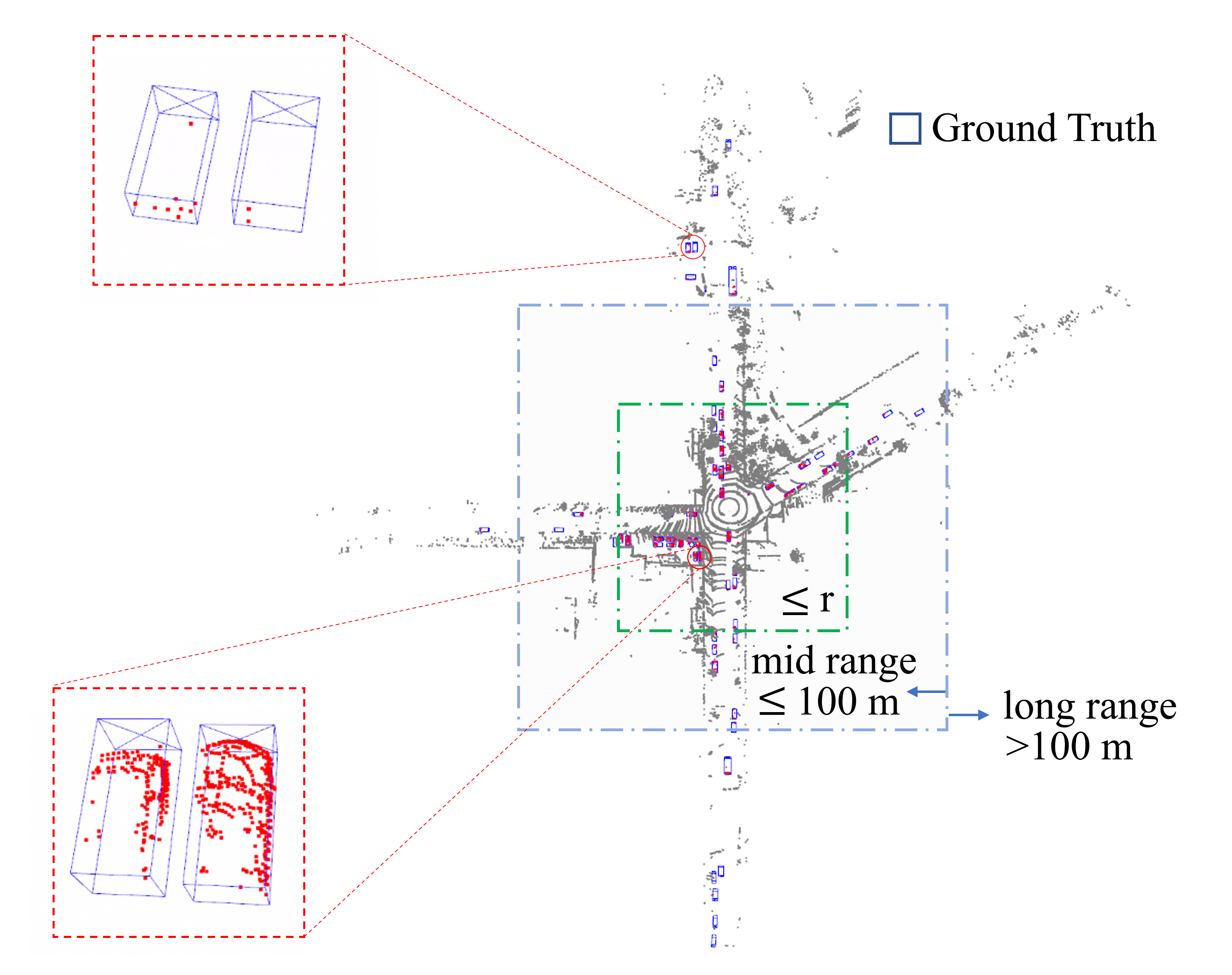
(a)

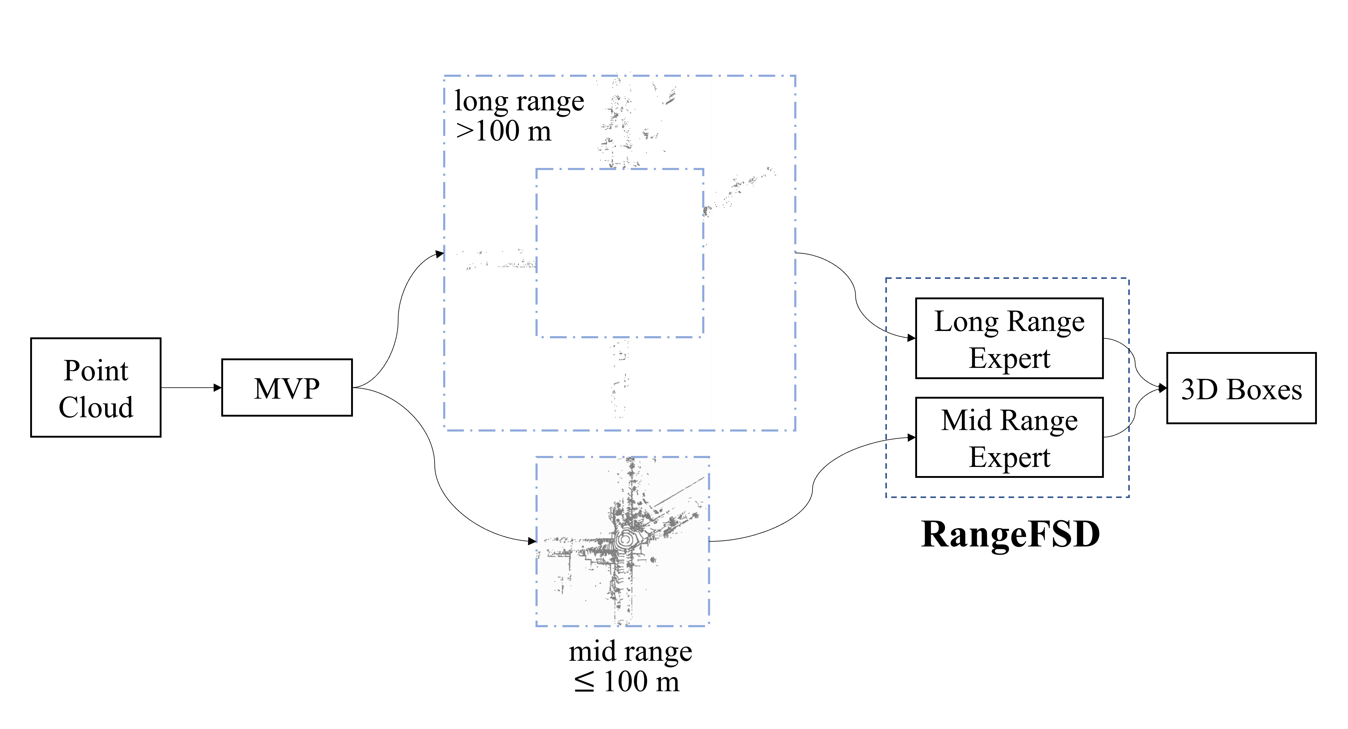
(b)

Figure 2: Increased LiDAR sparsity with distance from ego vehicle is one of the major challenges facing long range (¿100 $\mathrm{m}$) 3D object detection. (a) shows that the two vehicles parked far away from the ego vehicle have fewer LiDAR points, as well as appear different compared to those parked nearby. To address this problem, we train two neural networks, one specializing in mid-range object detection, and one for detecting long-range objects. The parameter $r\in[0,250]$, represented by the green box, delimits a subset of points used for training a specific expert. Mid-range experts use points within a distance $r$ of the ego vehicle, while points outside this box are used to train the long-range experts. (b) During inference, we combine outputs from the two networks, such that the long-range detector contributes detections beyond blue box (¿100 $\mathrm{m}$), and the mid-range detector contributes detections within blue box.

The first issue is that the LiDAR point cloud gets increasingly sparse with distance. This causes a form of domain gap, which has been studied in the context of sim2real or sensor-to-sensor mapping applications [6], but not with regards to long range detection. Studies have suggested relying on camera-based methods for object detection beyond a specific range [5]. Alternatively, utilization of a dedicated network designed for processing long-range point data has been proposed [4]. Another consequence of LiDAR sparsity is that a LiDAR based detector lacks the necessary information to make precise predictions.

The second issue is related to the uneven distribution of labeled objects across different ranges for training. Partially as a result of increasing LiDAR sparsity with distance, there are fewer annotations at long-range, as shown in  Figure 1. Although many new datasets have been released covering long-range annotations partially, they do not specifically focus on improving label imbalance for long-range annotations [7, 8, 9, 10].

These shortcomings underscore the significance of our contributions:

• To mitigate the problem of LiDAR sparsity, we leverage recent developments in image based depth completion, and generate virtual points for objects selected by an image based segmentation network. An increased density of points is found to benefit both mid and long-range detection results

• Although depth completion reduces the domain gap between mid-range and long-range objects, it doesn’t remove it completely. To further address this issue, we train two networks as range experts, one specializing on mid range, and one learning long-range detections. During inference, we combine outputs from these networks such that they only detect objects in their respective range domains. (an overview of our proposed detection pipeline is shown in Figure 2).

• To tackle the challenge of label imbalance, we propose an innovative range-adaptive label weighing scheme. During training, higher weightage is assigned to the loss component of a faraway labeled object compared to the one nearer to the ego vehicle. This weighing is inversely proportional to the number of annotations in a particular range bin.

• We combine long-range expert trained with range-adaptive weights, and a mid-range expert. Both are trained using depth completed point cloud data. This results in a state-of-the-art performance on the AV2 dataset, with improvements at long range. To our best knowledge, we are the first to provide a comprehensive evaluation of 3D object detectors beyond 100 meters range.

The rest of this article is structured as follows. Section II describes the related work in the field of 3D Object Detection, with a focus on long range detection. Section III describes range experts and outlines a novel training scheme for long range detection. Section IV presents the experimental results and discusses their implications, while limitations, concluding remarks and future work are discussed in Section V and VI.

II Related Work

This section presents the state-of-the-art in long-range 3D object detection and image based depth completion, as well as briefly describes the methods in fully sparse detection, most related to our work.

II-A Long Range 3D Object Detection

Point based or grid based methods utilizing sparse convolutions [11, 12] present interesting opportunities for long range 3D detection. VoxelNext [13] adds downsampling layers to existing 3D sparse convolution blocks to enlarge the receptive field, followed by pruning voxels with low feature magnitude, striking a balance between performance and computation. IA-SSD [14] first estimates per-point semantics and a centroid aware feature indicating closeness to a box center, and uses it to sample top $k$ points. While both methods demonstrate generally good performance, the feature pruning might remove information for long range objects.

Recently, there has been growing interest in multimodal fusion based methods for long range detection. In Far3Det [5], the authors report that fusion based methods outperform LiDAR only methods, given that the inaccuracies in camera based depth estimation are taken into account during evaluation. They propose range adaptive NMS thresholds and a straight-forward late fusion scheme, where camera-based detections are preferred beyond certain range. However, at present many camera based methods for 3D detection rely on converting image features into bird’s eye view (BEV) representations, which poses significant computational challenges for long range [15]. Zhang et. al. [4] classify and cluster the points inside frustum obtained from image based segmentation networks, and design a novel FFNet to regress the 3D bounding box. Fully Sparse Fusion (FSF) [3] similarly uses image to cluster LiDAR points. They further utilize the Fully Sparse Detector (FSD) [16] network to filter noisy points at mask boundaries. The image segmented cluster is fused with LiDAR segmented clusters for feature extraction and box prediction. To the best of our understanding, none of the methods listed above discuss or present results specifically at long range, i.e. above 100 $\mathrm{m}$ distance.

II-B Fully Sparse Detectors

FSD [16] is among the first computationally efficient point based methods. It overcomes the drawbacks of neighborhood querying and multiple cluster assignments faced by previous methods, by first pre-segmenting and voting on the point cloud using a SparseUNet [12]. Clustering [17] on these voted centers assigns a unique grouping to every point, avoiding ambiguity. This is followed by designing a novel Sparse Instance Recognition (SIR) module to extract cluster features and predict boxes.

To account for noise in clustering, FSD v2 [18] instead voxelizes the voted centers to form virtual voxels to capture the ambiguity/noise in clustering. Thereafter multi-scale features from a sparseUNet decoder are fused with those from virtual voxels and real voxels (obtained from the foreground segmented points). We use FSD and FSD v2 as backbones for mid range and long range experts, due to their state-of-the-art results on long range 3D object detection, as well as their computational efficiency. Our method further improves the performance of these models, making them, to our best knowledge, the current state-of-the-art results with improvements both at mid and long ranges.

II-C Image Based Depth Completion

Rich semantic information from image based 2D detectors can provide valuable cues for long range objects, such as rough estimation of object center [4, 19], enhanced feature representations [20, 21], etc. An intriguing research direction, which directly addresses the LiDAR sparsity problem is image-based depth completion. Prior research has explored this approach to a lesser extent in the context of long-range 3D detection. In the work reported in [22], a Deep Neural Network (DNN) is used to estimate surface normals and occlusion boundaries, and combine them with raw depth measurements for depth completion. The work presented in [23] uses classical image processing operations like dilation with custom designed kernel, hole filling, and median filtering to fill the depth map. The method Multimodal Virtual Points (MVP) [24] first uses an image based instance segmentation network to generate instance masks where $s$ pixels are randomly sampled without repetition for each mask. Next, for each pixel, the nearest LiDAR point, obtained by projecting the point cloud onto mask using intrinsic and extrinsic parameters, is located. The nearest LiDAR points are then used to assign depth to these $s$ pixels, which are lastly unprojected back to 3D to obtain the virtual points. Among existing approaches, the MVP stands out as one of the top-performing methods, notable for its efficacy and simplicity. We use MVP to generate virtual points, which we combine with the LiDAR points before training our range experts.

III Methodology

In order to improve performance on long-range points, two different approaches are used: range thresholding and range weighing. To address the LiDAR sparsity problem, we also evaluate the impact of MVP to generate virtual LiDAR points at all ranges and combine them with real points for training. Finally, we combine our best performing range experts into our final state-of-the-art model.

III-A Notation

The set $\mathcal{P}=\{(x_{i},y_{i},z_{i},f_{i}),i\in\mathbb{N}\}$ represents a point cloud in $\mathbb{R}^{4}$. Range experts are denoted by F${}_{r_{1}-r_{2}}$ where F is the DNN used for training, and $r_{1},r_{2}\in\mathcal{R}=\{0,50,100,150,200,250\}$ are the range thresholds (in meters) within which it is trained. For a range threshold $r$, we consider a square axis aligned region where $r$ denotes the distance from the origin to the border along the x or y axis. The set $\mathcal{R}$ further defines a set of bins $\mathcal{B}$ separated by fixed length interval of 50 $\mathrm{m}$. The maximum range is set to 250 $\mathrm{m}$ for the AV2 dataset. Specifically, F${}_{r_{1}-r_{2}}$ is trained to perform inference for points $p\in\mathcal{P}$ such that $r_{1}\leq r\leq r_{2}$, and we investigate which ranges should be used for training. In this paper, we consider F_0-250 as the baseline model upon which we build our contributions.

III-B Range Experts

Due to the increase in sparsity of the LiDAR point cloud as a function of the distance, objects at different distances appear to be radically different. We use range thresholding to target objects in different domains. Range thresholding consists of training the network using only a subset of points within a specific range interval $r_{1}-r_{2}$. The resulting networks are referred to as range experts.

In this paper, we compare range experts specialised on object detection at mid and long range with those trained on the full dataset, referred to as general. Given the large difference in the number of labeled objects as a function of their distance, which was illustrated in Fig. 1, a mid-range expert is not crucial since the baseline, F_0-250, already performs fairly well as a mid-range detector, however, specialised long-range experts are clearly required. We evaluate the performance of the long-range experts as a function of the range thresholding values. Similarly to [25], which tests range thresholds on BEV methods, we observe that as we increase the lower bound for range thresholding, the network performs poorer compared to baseline at long range. This is because, as seen in Fig. 1, we end up discarding larger and larger proportion of labels while training, and the network doesn’t have enough data to learn from. This problem inspired us to also implement the range adaptive weighing.

III-C Range Adaptive Weighing

Range weighing is aimed at compensating for the imbalance of labeled objects at large distances, which was illustrated in Fig. 1. This is achieved by increasing the impact of objects that are further away on the loss function. In order to strike a balance between range thresholding and retaining sufficient labels for training, we propose range adaptive weighing. The loss corresponding to a predicted cluster/virtual voxel is weighed according to its range. In general, the label weight $w_{b}$ for the range bin $b$ is given by:

$$w_{b}=\frac{N}{n_{b}\times B}$$ (1)

where $N$ is the total number of labels for all classes in the dataset, $n_{b}$ is the number of objects in range bin $b$ and $B$ is the number of bins covered by the range expert. The weight $w_{b}$ is applied to the Focal Loss [26] and $L_{1}$ Loss [27], which are used as classification and regression losses for the prediction head for bounding boxes. The other loss terms remain unchanged (refer to [16], [18] for more details). We denote F${}_{r_{1}-r_{2}}^{w}$ as an expert trained using range weighing.

III-D Late Fusion

We study various combinations of range thresholding and range weighing in Section IV-B, using FSD [16]. Based on that, we choose F_0-100 and F${}_{50-250}^{w}$ as best performing mid and long range experts, where F^w denotes range wighted model. We finetune our models using virtual points generated by MVP for these configurations and combine them into a single network, as shown in Fig. 2(b). Consequently, FSD_0-100 and FSD${}_{50-250}^{w}$ form the mid and long-range experts of a single network, which we refer to as RangeFSD. Similarly, we obtain another network RangeFSDv2, with FSDv2 [18] as backbone.

During inference, the detections from the mid and long-range experts are combined such that the mid-range expert contributes detections with centers from 0-100 meters, whereas the long-range expert contributes detections from 100-250 meters.

IV Experiments

A variety of experiments and ablation studies are documented in this section. We assess the impact of our individual contributions to our final state-of-the-art model and compare it to other models from the literature.

IV-A Experimental Setup

Dataset: We conduct experiments on the AV2 perception dataset, which contains 1000 scenes divided into 700 for training and 150 each for validation and testing. Each scene captures roughly 15 $\mathrm{s}$ of data on two 32-beam LiDARs at 10 $\mathrm{H}\mathrm{z}$ but with a 180^∘ difference in spinning angle, seven color cameras and two forward-facing stereo cameras at 20 $\mathrm{H}\mathrm{z}$, providing a surround view of the vehicle. Objects of interest are annotated at 10 $\mathrm{H}\mathrm{z}$ among 30 categories, up to 225 $\mathrm{m}$ away from the ego vehicle.

Implementation Details: We base our implementation on FSD [16], which is in turn developed using mmdetection3d library [28]. We use Hybrid Task Cascade (HTC) [29] pretrained on NuImages dataset as the default 2D image segmentor for generating the virtual points. We start with a pre-trained FSD and train for six epochs using Class-balanced grouping and sampling (CBGS) [30]. Thereafter, we enable MVP and train further using CBGS for three epochs. We use the same data augmentations and learning parameters as FSD and train on eight Nvidia A-100 GPUs.

Metrics: AV2 uses mean Average Precision (mAP) and Composite Detection Score (CDS) scores for evaluating 3D detection. In this work, we report the mAP, which is defined as the mean of Average Precision (AP) across $C$ classes, where AP _j for class $j$ is the discrete integral of precision $p_{d}(a)$ interpolated at 100 discrete recall values $a\in[0,1]$, averaged across four chosen distance thresholds $d$ (in meters).

$$mAP =\frac{1}{C}\sum^{C}_{j=1}AP_{j}$$ (2)

$$AP_{j} =\frac{1}{4}\sum_{d=\{0.5,1,2,4\}}\frac{1}{100}\sum_{a=\{0,0.05,\ldots,1\}}p_{d}(a)$$ (3)

Unless otherwise specified, we use an evaluation range of 0-250 $\mathrm{m}$ in our experiments.

IV-B Strategies for Training Long Range Detector

TABLE I: Effect of Range thresholding and range weighing on mAP.

		Range
Expert	Method	Weights	0-250	0-50	50-100	100-150	150-200	200-250
General	FSD0-250	$-$	31.5	46.4	16.6	5.4	1.8	0.5
	FSD${}_{0-250}^{w}$	✓	31.3	45.9	17.0	5.7	1.8	0.4
Mid	FSD0-100 *	$-$	31.3	46.9	16.9	0.5	-	-
Long	FSD50-250	$-$	6.1	-	16.6	5.9	2.0	0.6
	FSD${}_{50-250}^{w}$ *	✓	6.0	-	16.5	6.1	2.0	0.5
	FSD100-250	$-$	1.0	-	-	4.9	2.0	0.6
	FSD${}_{100-250}^{w}$	✓	1.1	-	-	5.0	2.1	0.5
Merged	$RangeFSD^{*}$	✓	31.9	46.9	16.9	5.8	2.0	0.5

The effect of range threshold and range weighing on the FSD trained using MVP is summarised in Table I. The general experts are optimised to target objects in the full 0-250 $\mathrm{m}$ range while the long- (mid-) range experts aim to maximise the performance for distances $>$ ($\leq$) 100 $\mathrm{m}$.  Table II further denotes the range weights for both mid and long range experts for different values of range thresholding $r_{1}$ and $r_{2}$. These weights are computed using Eq. 1 together with the the bin-wise label statistics of the training set, which were shown in Fig. 1.

TABLE II: Range weights for different values of range thresholds. $r_{1}$ and $r_{2}$ are lower and upper limits for thresholding.

$r_{1}$	$r_{2}$	0-50	50-100	100-150	150-200	200-250
0	250	0.360	0.661	1.852	6.486	52.332
50	250	0	0.367	1.030	3.607	29.103
100	250	0	0	0.440	1.542	12.440

The range weights, which are implemented in FSD${}_{0-250}^{w}$, show a performance improvement in the 50-150 $\mathrm{m}$ range with respect to FSD_0-250 and a performance degrading in the below 50 $\mathrm{m}$ range. We also train long-range experts using range thresholding of $50-250$ $\mathrm{m}$ and $100-250$ $\mathrm{m}$ with and without range weights for comparison. In particular, FSD_100-250 corresponds to simply finetuning the network for long-range points, and it performs the worst in 100-150 $\mathrm{m}$ range. It is observed that range weighing leads to slight improvements for both long-range experts. Moreover, it is found that the best performance for a range bin $b$ can be obtained by using range thresholding from bin $b-1$ in combination with range weighing i.e. the best performance at $100-150$ $\mathrm{m}$ is obtained by FSD${}_{50-250}^{w}$. We also train a short range expert, referred as FSD_0-100, using range thresholding of $0-100$ $\mathrm{m}$. Range weights are not applied in this case in order not to degrade the performance at $0-50$ $\mathrm{m}$. As expected, the short range expert results in the most optimal performance for objects at $0-50$ $\mathrm{m}$, while the performance at $50-100$ $\mathrm{m}$ is only degraded by 0.1% with respect to FSD${}_{0-250}^{w}$. Based on the results, we choose FSD_0-100 and FSD${}_{50-250}^{w}$ as the mid- and long- range experts, and merge them to form RangeFSD, a network with high performance at both mid and long range.

IV-C Performance Breakdown

Our contribution can be divided into two components: implementation of MVP and range experts. In order to assess the impact of each component on our final state-of-the art algorithms, a detailed performance breakdown, shown in Table III, is performed.

TABLE III: Performance breakdown for different settings.

Method	MVP	0-250	0-50	50-100	100-150	150-200	200-250
FSD	$-$	29.8	44.9	14.3	4.1	1.0	0.3
	✓	31.5	46.4	16.6	5.4	1.8	0.5
RangeFSD	$-$	30.2	45.5	14.8	4.6	1.2	0.3
	✓	31.9	46.9	16.9	5.8	2.0	0.5

The impact of MVP is studied independently for the FSD and RangeFSD. It was observed that finetuning after adding virtual points is crucial for both the cases. A significant drop in performance is observed when applying MVP without finetuning. This drop could be explained by a shift in point distribution caused by MVP. The LiDAR pre-segmentor, used by both baselines, is negatively affected by this shift and hence needs to be finetuned. Overall, MVP contributes to about 1.7% increase in mAP, whereas the range expert contributes about 0.4% mAP. Although a higher boost in performance arises from MVP, a combination of MVP and range experts is required to maximise the performance of FSD.

IV-D Comparison to Baseline

TABLE IV: mAP comparison to Baseline. $\dagger$: provided by authors [16][18]. *: re-trained by us.

Method	0-250	0-50	50-100	100-150	150-200	200-250
FSD$\dagger$	28.5	43.7	12.6	3.3	1.0	0.3
FSD*	29.8	44.9	14.3	4.1	1.0	0.3
RangeFSD	31.9	46.9	16.9	5.8	2.0	0.5
FSDv2$\dagger$	37.5	52.8	22.3	7.5	2.5	0.4
FSDv2*	37.5	52.2	23.0	8.6	2.5	0.5
RangeFSDv2	38.3	52.3	25.2	9.8	3.1	0.6

A comparison between our algorithms and their respective baselines as a function of the range is shown in Table IV. To guarantee a fair comparison, we re-train the baseline networks for six epochs using CBGS, which we denote by $*$. We also provide the performance reported by the authors of the baseline for completeness, denoted by $\dagger$. For FSD, we reduce the minimum points for clustering from two to one, to enable clustering at long range. It’s observed that using CBGS seems to slightly benefit long range performance. For both baselines, a consistent improvement across ranges can be attributed to the respective range experts specializing in their domain. Nevertheless, very little improvement is observed in 200-250$\mathrm{m}$ range, perhaps because labels in this range constitute only 0.3% of the dataset, as shown in Fig. 1. Our results underscore the substantial room for improvement within the current state-of-the-art for long-range 3D detection.

IV-E State-of-the-art Comparison

TABLE V: Comparison to state-of-the-art on AV2 validation split. The evaluation range is 0-200 $\mathrm{m}$. $\dagger$: provided by authors of AV2 [2]. $\ddagger$: reimplemented by FSD [16]. C-Barrel: construction barrel, MPC-Sign: mobile pedestrian crossing sign, A-Bus: articulated bus, C-Cone: construction cone, V-Trailer: vehicular Trailer, W-Device: wheeled device, W-Rider: wheeled rider.

Method	mAP	Vehicle	Bus	Pedestrian	Stop Sign	Box Truck	Bollard	C-Barrel	Motorcyclist	MPC-Sign	Motorcycle	Bicycle	A-Bus	School Bus	Truck Cab	C-Cone	V-Trailer	Sign	Large Vehicle	Stroller	Bicyclist	Truck	MBT	Dog	Wheelchair	W-Device	W-Rider
CenterPoint$\dagger$ [31]	13.5	61.0	36.0	33.0	28.0	26.0	25.0	22.5	16.0	16.0	12.5	9.5	8.5	7.5	8.0	8.0	7.0	6.5	3.0	2.0	14.0	14.0	1.0	0.5	0	3.0	0
CenterPoint$\ddagger$	22.0	67.6	38.9	46.5	16.9	37.4	40.1	32.2	28.6	27.4	33.4	24.5	8.7	25.8	22.6	29.5	22.4	6.3	3.9	0.5	20.1	22.1	0	3.9	0.5	10.9	4.2
VoxelNeXt [13]	30.7	72.7	38.8	63.2	40.2	40.1	53.9	64.9	44.7	39.4	42.4	40.6	20.1	25.2	19.9	44.9	20.9	14.9	6.8	15.7	32.4	16.9	0	14.4	0.1	17.4	6.6
FSF [3]	33.2	70.8	44.1	60.8	27.7	40.2	41.1	50.9	48.9	28.3	60.9	47.6	22.7	36.1	26.7	51.7	28.1	12.2	6.8	25.0	41.6	-	-	-	-	-	-
FSD [16]	28.2	68.1	40.9	59.0	29.0	38.5	41.8	42.6	39.7	26.2	49.0	38.6	20.4	30.5	14.8	41.2	26.9	11.9	5.9	13.8	33.4	21.1	0	9.5	7.1	14.0	9.2
RangeFSD∗	31.9	74.5	42.1	69.2	32.0	39.1	53.3	58.7	50.1	27.4	55.9	46.1	21.2	30.5	20.2	54.8	26.4	12.0	6.2	15.9	42.6	21.4	0	1.9	2.3	17.2	9.5
FSDv2 [18]	37.6	77.0	47.6	70.5	43.6	41.5	53.9	58.5	56.8	39.0	60.7	49.4	28.4	41.9	30.2	44.9	33.4	16.6	7.3	32.5	45.9	24.0	1.0	12.6	17.1	26.3	17.2
RangeFSDv2∗	38.5	78.5	48.4	72.8	43.0	41.5	56.1	65.1	60.2	48.8	63.8	53.2	29.6	40.6	30.3	55.9	31.3	16.2	7.3	30.3	48.9	23.8	0	14.6	1.4	25.0	14.7

The comparison of different state-of-the art algorithms is shown in Table V. Our algorithms, marked with ^∗, outperform their respective baselines, as well as all previous state-of-the-art methods. The evaluation range is set to 0-200 $\mathrm{m}$ to enable a fair comparison to other methods. Although improvements span across many classes, they are especially notable for vulnerable road users (2-3% for pedestrians, motorcyclist, bicyclist) and small objects (3-10% for motorcycle, bicycle and construction cones). Equally interesting is the drop in performance for some classes, as compared to FSD v2 baseline. This drop could be caused by the noise in the virtual point generation process, which in turn is caused by noisy masks generated by the 2D segmentor, for classes it is not trained on. As mentioned earlier, we use an off-the-shelf 2D segmentor (HTC [29]) trained on the NuImages dataset. We perform a one-to-one mapping between NuImage classes and their best match among the 26 classes in the AV2 dataset. Inevitably, some classes not covered by this scheme don’t improve (like box truck), or even get worse if mislabeled (eg. wheelchair, sign, stop sign etc.).

IV-F Effect of image segmentation

To analyze the impact of image segmentation backbone on the performance of our proposed approach, we replace HTC [29] (default 2D segmentor) with Mask RCNN [32], another well known image segmentor. As shown in Table VI, our finetuned RangeFSD with Mask RCNN gives similar results to HTC, demonstrating robustness to the 2D segmentor employed. On the other hand, the significantly higher mask and box mAP for HTC indicates that while both the segmentors seem to detect mid range objects equally well, HTC could be better at detecting small objects. Some of these small objects could very well be at large distances, outside the reach of LiDAR points, making it impossible for a LiDAR-only detector to detect them.

TABLE VI: Effect of 2D backbone on mAP performance.

Method	2D mAP		3D mAP
	Mask	Box
HTC [29]	46.4	57.3	31.9
Mask RCNN [32]	38.4	47.8	31.8

V Limitations

Firstly, we did not account for extrinsic calibration mismatches between LiDAR and cameras. Such misalignments can significantly affect object detection, particularly during depth completion, leading to erroneous depth estimations or even the exclusion of objects due to the absence of nearby lidar points. This limitation becomes especially pronounced for distant objects and can have a significant impact on our network’s performance. Secondly, the effects of fusing data from active LiDAR sensors with passive camera sensors, most of which employ rolling shutters, need to be further investigated. This limitation is especially pertinent when dealing with highly dynamic objects, as they can appear differently in each sensor’s data, leading to further mismatch during depth completion. Finally, We did not investigate scenarios where large objects, like trucks with trailers, span our range boundaries. In such cases, short-range and long-range networks may yield separate bounding boxes for the same object, necessitating fusion.

VI Conclusions and Future Work

In this work, we identify two key problems that 3D Object Detectors face at long range: LiDAR sparsity, causing a form of domain gap, and label imbalance between mid and long range objects. To address these problems, we propose a combination of fully sparse detectors (FSD and FSDv2) as range experts, trained using an adaptive range weighing scheme, and virtual points obtained from MVP, a powerful method for image based depth completion. Our network achieves a state-of-the-art performance on the AV2 dataset. Nevertheless, a large margin for improvement remains for ranges beyond 50 meters. One next step could be investigating whether deep image features could aid sparse LiDAR features for detection, while being computationally efficient. Another interesting line of investigation can be studying camera based methods to detect objects beyond the range of current LiDAR sensors.

References

- [1] S. Shalev-Shwartz, S. Shammah, and A. Shashua, “On a formal model of safe and scalable self-driving cars,” arXiv preprint arXiv:1708.06374, 2017.
- [2] B. Wilson, W. Qi, T. Agarwal, J. Lambert, J. Singh, S. Khandelwal, B. Pan, R. Kumar, A. Hartnett, J. K. Pontes et al., “Argoverse 2: Next generation datasets for self-driving perception and forecasting,” arXiv preprint arXiv:2301.00493, 2023.
- [3] Y. Li, L. Fan, Y. Liu, Z. Huang, Y. Chen, N. Wang, Z. Zhang, and T. Tan, “Fully sparse fusion for 3d object detection,” arXiv preprint arXiv:2304.12310, 2023.
- [4] H. Zhang, D. Yang, E. Yurtsever, K. A. Redmill, and Ü. Özgüner, “Faraway-frustum: Dealing with lidar sparsity for 3d object detection using fusion,” in 2021 IEEE International Intelligent Transportation Systems Conference (ITSC). IEEE, 2021, pp. 2646–2652.
- [5] S. Gupta, J. Kanjani, M. Li, F. Ferroni, J. Hays, D. Ramanan, and S. Kong, “Far3det: Towards far-field 3d detection,” in Proceedings of the IEEE/CVF Winter Conference on Applications of Computer Vision, 2023, pp. 692–701.
- [6] L. T. Triess, M. Dreissig, C. B. Rist, and J. M. Zöllner, “A survey on deep domain adaptation for lidar perception,” in 2021 IEEE intelligent vehicles symposium workshops (IV workshops). IEEE, 2021, pp. 350–357.
- [7] H. Caesar, V. Bankiti, A. H. Lang, S. Vora, V. E. Liong, Q. Xu, A. Krishnan, Y. Pan, G. Baldan, and O. Beijbom, “nuscenes: A multimodal dataset for autonomous driving,” in Proceedings of the IEEE/CVF conference on computer vision and pattern recognition, 2020, pp. 11 621–11 631.
- [8] P. Sun, H. Kretzschmar, X. Dotiwalla, A. Chouard, V. Patnaik, P. Tsui, J. Guo, Y. Zhou, Y. Chai, B. Caine et al., “Scalability in perception for autonomous driving: Waymo open dataset,” in Proceedings of the IEEE/CVF conference on computer vision and pattern recognition, 2020, pp. 2446–2454.
- [9] T. Matuszka, I. Barton, Á. Butykai, P. Hajas, D. Kiss, D. Kovács, S. Kunsági-Máté, P. Lengyel, G. Németh, L. Pető et al., “aimotive dataset: A multimodal dataset for robust autonomous driving with long-range perception,” arXiv preprint arXiv:2211.09445, 2022.
- [10] M. Alibeigi, W. Ljungbergh, A. Tonderski, G. Hess, A. Lilja, C. Lindstrom, D. Motorniuk, J. Fu, J. Widahl, and C. Petersson, “Zenseact open dataset: A large-scale and diverse multimodal dataset for autonomous driving,” arXiv preprint arXiv:2305.02008, 2023.
- [11] Y. Yan, Y. Mao, and B. Li, “Second: Sparsely embedded convolutional detection,” Sensors, vol. 18, no. 10, p. 3337, 2018.
- [12] B. Graham and L. Van der Maaten, “Submanifold sparse convolutional networks,” arXiv preprint arXiv:1706.01307, 2017.
- [13] Y. Chen, J. Liu, X. Zhang, X. Qi, and J. Jia, “Voxelnext: Fully sparse voxelnet for 3d object detection and tracking,” in Proceedings of the IEEE/CVF Conference on Computer Vision and Pattern Recognition, 2023, pp. 21 674–21 683.
- [14] Y. Zhang, Q. Hu, G. Xu, Y. Ma, J. Wan, and Y. Guo, “Not all points are equal: Learning highly efficient point-based detectors for 3d lidar point clouds,” in Proceedings of the IEEE/CVF Conference on Computer Vision and Pattern Recognition, 2022, pp. 18 953–18 962.
- [15] X. Jiang, S. Li, Y. Liu, S. Wang, F. Jia, T. Wang, L. Han, and X. Zhang, “Far3d: Expanding the horizon for surround-view 3d object detection,” arXiv preprint arXiv:2308.09616, 2023.
- [16] L. Fan, F. Wang, N. Wang, and Z.-X. ZHANG, “Fully sparse 3d object detection,” Advances in Neural Information Processing Systems, vol. 35, pp. 351–363, 2022.
- [17] L. He, X. Ren, Q. Gao, X. Zhao, B. Yao, and Y. Chao, “The connected-component labeling problem: A review of state-of-the-art algorithms,” Pattern Recognition, vol. 70, pp. 25–43, 2017.
- [18] L. Fan, F. Wang, N. Wang, and Z. Zhang, “FSD V2: Improving Fully Sparse 3D Object Detection with Virtual Voxels,” arXiv preprint arXiv:2308.03755, 2023.
- [19] C. R. Qi, X. Chen, O. Litany, and L. J. Guibas, “Imvotenet: Boosting 3d object detection in point clouds with image votes,” in Proceedings of the IEEE/CVF conference on computer vision and pattern recognition, 2020, pp. 4404–4413.
- [20] S. Vora, A. H. Lang, B. Helou, and O. Beijbom, “Pointpainting: Sequential fusion for 3d object detection,” in Proceedings of the IEEE/CVF conference on computer vision and pattern recognition, 2020, pp. 4604–4612.
- [21] S. Xu, D. Zhou, J. Fang, J. Yin, Z. Bin, and L. Zhang, “Fusionpainting: Multimodal fusion with adaptive attention for 3d object detection,” in 2021 IEEE International Intelligent Transportation Systems Conference (ITSC). IEEE, 2021, pp. 3047–3054.
- [22] Y. Zhang and T. Funkhouser, “Deep depth completion of a single rgb-d image,” in Proceedings of the IEEE conference on computer vision and pattern recognition, 2018, pp. 175–185.
- [23] J. Ku, A. Harakeh, and S. L. Waslander, “In defense of classical image processing: Fast depth completion on the cpu,” in 2018 15th Conference on Computer and Robot Vision (CRV). IEEE, 2018, pp. 16–22.
- [24] T. Yin, X. Zhou, and P. Krähenbühl, “Multimodal virtual point 3d detection,” Advances in Neural Information Processing Systems, vol. 34, pp. 16 494–16 507, 2021.
- [25] N. Peri, M. Li, B. Wilson, Y.-X. Wang, J. Hays, and D. Ramanan, “An empirical analysis of range for 3d object detection,” arXiv preprint arXiv:2308.04054, 2023.
- [26] T.-Y. Lin, P. Goyal, R. Girshick, K. He, and P. Dollár, “Focal loss for dense object detection,” in Proceedings of the IEEE international conference on computer vision, 2017, pp. 2980–2988.
- [27] R. Girshick, “Fast r-cnn,” in Proceedings of the IEEE international conference on computer vision, 2015, pp. 1440–1448.
- [28] M. Contributors, “MMDetection3D: OpenMMLab next-generation platform for general 3D object detection,” https://github.com/open-mmlab/mmdetection3d, 2020.
- [29] K. Chen, J. Pang, J. Wang, Y. Xiong, X. Li, S. Sun, W. Feng, Z. Liu, J. Shi, W. Ouyang et al., “Hybrid task cascade for instance segmentation,” in Proceedings of the IEEE/CVF conference on computer vision and pattern recognition, 2019, pp. 4974–4983.
- [30] B. Zhu, Z. Jiang, X. Zhou, Z. Li, and G. Yu, “Class-balanced grouping and sampling for point cloud 3d object detection,” arXiv preprint arXiv:1908.09492, 2019.
- [31] T. Yin, X. Zhou, and P. Krahenbuhl, “Center-based 3d object detection and tracking,” in Proceedings of the IEEE/CVF conference on computer vision and pattern recognition, 2021, pp. 11 784–11 793.
- [32] K. He, G. Gkioxari, P. Dollár, and R. Girshick, “Mask r-cnn,” in Proceedings of the IEEE international conference on computer vision, 2017, pp. 2961–2969.