Accelerate Multi-Agent Reinforcement Learning in Zero-Sum Games with Subgame Curriculum Learning

Abstract

Learning Nash equilibrium (NE) in complex zero-sum games with multi-agent reinforcement learning (MARL) can be extremely computationally expensive. Curriculum learning is an effective way to accelerate learning, but an under-explored dimension for generating a curriculum is the difficulty-to-learn of the subgames – games induced by starting from a specific state. In this work, we present a novel subgame curriculum learning framework for zero-sum games. It adopts an adaptive initial state distribution by resetting agents to some previously visited states where they can quickly learn to improve performance. Building upon this framework, we derive a subgame selection metric that approximates the squared distance to NE values and further adopt a particle-based state sampler for subgame generation. Integrating these techniques leads to our new algorithm, Subgame Automatic Curriculum Learning (SACL), which is a realization of the subgame curriculum learning framework. SACL can be combined with any MARL algorithm such as MAPPO. Experiments in the particle-world environment and Google Research Football environment show SACL produces much stronger policies than baselines. In the challenging hide-and-seek quadrant environment, SACL produces all four emergent stages and uses only half the samples of MAPPO with self-play. The project website is at https://sites.google.com/view/sacl-rl.

Introduction

Applying reinforcement learning (RL) to zero-sum games has led to enormous success, with trained agents defeating professional humans in Go (Silver et al. 2016), StarCraft II (Vinyals et al. 2019), and Dota 2 (Berner et al. 2019). To find an approximate Nash equilibrium (NE) in complex games, these works often require a tremendous amount of training resources including hundreds of GPUs and weeks or even months of time. The unaffordable cost prevents RL from more real-world applications beyond these flagship projects supported by big companies and makes it important to develop algorithms that can learn close-to-equilibrium strategies in a substantially more efficient manner.

One way to accelerate training is curriculum learning – training agents in tasks from easy to hard. Many existing works in solving zero-sum games with MARL generate a curriculum by choosing whom to play with. They often use self-play to provide a natural policy curriculum as the agents are trained against increasingly stronger opponents (Bansal et al. 2018; Baker et al. 2020). The self-play framework can be further extended to population-based training (PBT) by maintaining a policy pool and iteratively training new best responses to mixtures of previous policies (McMahan, Gordon, and Blum 2003; Lanctot et al. 2017). Such a policy-level curriculum generation paradigm is very different from the paradigm commonly used in goal-conditioned RL (Matiisen et al. 2019; Portelas et al. 2020). Most curriculum learning methods for goal-conditioned problems directly reset the goal or initial states for each training episode to ensure the current task is of suitable difficulty for the learning agent. In contrast, the policy-level curriculum in zero-sum games only provides increasingly stronger opponents, and the agents are still trained by playing the full game starting from a fixed initial state distribution, which is often very challenging.

In this paper, we propose a general subgame curriculum learning framework to further accelerate MARL training for zero-sum games. It leverages ideas from goal-conditioned RL. Complementary to policy-level curriculum methods like self-play and PBT, our framework generates subgames (i.e., games induced by starting from a specific state) with growing difficulty for agents to learn and eventually solve the full game. We provide justifications for our proposal by analyzing a simple iterated Rock-Paper-Scissors game. We show that in this game, vanilla MARL requires exponentially many samples to learn the NE. However, by using a buffer to store the visited states and choosing an adaptive order of state-induced subgames to learn, the NE can be learned with linear samples.

A key challenge in our framework is to choose which subgame to train on. This is non-trivial in zero-sum games since there does not exist a clear progression metric like the success rate in goal-conditioned problems. While the squared difference between the current state value and the NE value can measure the progress of learning, it is impossible to calculate this value during training as the NE is generally unknown. We derive an alternative metric that approximates the squared difference with a bias term and a variance term. The bias term measures how fast the state value changes and the variance term measures how uncertain the current value is. We use the combination of the two terms as the sampling weights for states and prioritize subgames with fast change and high uncertainty. Instantiating our framework with the state selection metric and a non-parametric subgame sampler, we develop an automatic curriculum learning algorithm for zero-sum games, i.e., Subgame Automatic Curriculum Learning (SACL). SACL can adopt any MARL algorithm as its backbone and preserve the overall convergence property. In our implementation, we choose the MAPPO algorithm (Yu et al. 2021) for the best empirical performances.

We first evaluate SACL in the Multi-Agent Particle Environment and Google Research Football, where SACL learns stronger policies with lower exploitability than existing MARL algorithms for zero-sum games given the same amount of environment interactions. We then stress-test the efficiency of SACL in the challenging hide-and-seek environment. SACL leads to the emergence of all four phases of different strategies and uses 50% fewer samples than MAPPO with self-play.

Preliminary

Markov Game

A Markov game (Littman 1994) is defined by a tuple $\mathcal{MG}=(\mathcal{N},\mathcal{S},\bm{\mathcal{A}},P,\bm{R},\gamma,\rho)$, where $\mathcal{N}=\{1,2,\cdots,N\}$ is the set of agents, $\mathcal{S}$ is the state space, $\bm{\mathcal{A}}=\Pi_{i=1}^{N}\mathcal{A}_{i}$ is the joint action space with $\mathcal{A}_{i}$ being the action space of agent $i$, $P:\mathcal{S}\times\bm{\mathcal{A}}\rightarrow\Delta(\mathcal{S})$ is the transition probability function, $\bm{R}=(R_{1},R_{2},\cdots,R_{N}):\mathcal{S}\times\bm{\mathcal{A}}\rightarrow\mathbb{R}^{n}$ is the joint reward function with $R_{i}$ being the reward function for agent $i$, $\gamma$ is the discount factor, and $\rho$ is the distribution of initial states. Given the current state $s$ and the joint action $\bm{a}=(a_{1},a_{2},\cdots,a_{N})$ of all agents, the game moves to the next state $s^{\prime}$ with probability $P(s^{\prime}|s,\bm{a})$ and agent $i$ receives a reward $R_{i}(s,\bm{a})$.

For infinite-horizon Markov games, a subgame $\mathcal{MG}(s)$ is defined as the Markov game induced by starting from state $s$, i.e., $\rho(s)=1$. Selecting subgames is therefore equivalent to setting the Markov game’s initial states. The subgames of finite-horizon Markov games are defined similarly and have an additional variable to denote the current step $t$.

We focus on two-player zero-sum Markov games, i.e., $N=2$ and $R_{1}(s,\bm{a})+R_{2}(s,\bm{a})=0$ for all state-action pairs $(s,\bm{a})\in\mathcal{S}\times\bm{\mathcal{A}}$. We use the subscript $i$ to denote variables of player $i$ and the subscript $-i$ to denote variables of the player other than $i$. Each player uses a policy $\pi_{i}:\mathcal{S}\rightarrow\mathcal{A}_{i}$ to produce actions and maximize its own accumulated reward. Given the joint policy $\bm{\pi}=(\pi_{1},\pi_{2})$, each player’s value function of state $s$ and Q-function of state-action pair $(s,\bm{a})$ are defined as

$$V^{\bm{\pi}}_{i}(s) =\mathbb{E}\Big{[}\sum_{t}\gamma^{t}R_{i}(s^{t},\bm{a}^{t})\Big{|}s^{0}=s\Big{]},$$ (1)

$$Q^{\bm{\pi}}_{i}(s,\bm{a}) =\mathbb{E}\Big{[}\sum_{t}\gamma^{t}R_{i}(s^{t},\bm{a}^{t})\Big{|}s^{0}=s,\bm{a}^{0}=\bm{a}\Big{]}.$$ (2)

The solution concept of two-player zero-sum Markov games is Nash equilibrium (NE), a joint policy where no player can get a higher value by changing the policy alone.

Definition 1 (NE).

A joint policy $\bm{\pi}^{*}=(\pi_{1}^{*},\pi_{2}^{*})$ is a Nash equilibrium of a Markov game if for all initial states $s^{0}$ with $\rho(s^{0})>0$, the following condition holds

$$\pi_{i}^{*}=\operatorname*{arg\,max}_{\pi_{i}}V_{i}^{(\pi_{i},\pi_{-i}^{*})}(s^{0}),\ \forall i\in\{1,2\}.$$ (3)

We use $V^{*}_{i}(\cdot)$ to denote the NE value function of player $i$ and $Q^{*}_{i}(\cdot,\cdot)$ to denote the NE Q-function of player $i$, and the following equations hold by definition and the minimax nature of zero-sum games.

$$V^{*}_{i}(s) =\max_{\pi_{i}}\min_{\pi_{-i}}\mathbb{E}_{\bm{a}\sim\bm{\pi}(\cdot|s)}\left[Q^{*}_{i}(s,\bm{a})\right],$$ (4)

$$Q^{*}_{i}(s,\bm{a}) =R_{i}(s,\bm{a})+\gamma\cdot\mathbb{E}_{s^{\prime}\sim P(\cdot|s,\bm{a})}\left[V^{*}_{i}(s^{\prime})\right].$$ (5)

MARL Algorithms in Zero-Sum Games

MARL methods have been applied to zero-sum games tracing back to the TD-Gammon project (Tesauro 1995). A large body of work (Zinkevich et al. 2007; Brown et al. 2019; Steinberger, Lerer, and Brown 2020; Gruslys et al. 2020) is based on regret minimization, and a well-known result is that the average of policies produced by self-play of regret-minimizing algorithms converges to the NE policy of zero-sum games (Freund and Schapire 1996). Another notable line of work (Littman 1994; Heinrich, Lanctot, and Silver 2015; Lanctot et al. 2017; Perolat et al. 2022) combines RL algorithms with game-theoretic approaches. These works typically use self-play or population-based training to collect samples and then apply RL methods like Q-learning (Watkins and Dayan 1992) and PPO (Schulman et al. 2017) to learn the NE value functions and policies, and have recently achieved great success (Silver et al. 2016; Jaderberg et al. 2018; Vinyals et al. 2019; Berner et al. 2019).

For the analysis in the next section, we introduce a classic MARL algorithm named minimax-Q learning (Littman 1994) that extends Q-learning to zero-sum games. Initializing functions $Q_{i}(\cdot,\cdot)$ with zero values, minimax-Q uses an exploration policy induced by the current Q-functions to collect a batch of samples $\{(s^{t},\bm{a}^{t},r_{i}^{t},s^{t+1})\}_{t=0}^{T}$ and uses these samples to update the Q-functions by

$$Q_{i}(s^{t},\bm{a}^{t})\leftarrow(1-\alpha)\cdot Q_{i}(s^{t},\bm{a}^{t})+\\ \alpha\cdot\big{(}r_{i}^{t}+\gamma\cdot\max_{\pi_{i}}\min_{\pi_{-i}}\mathbb{E}_{\bm{a}\sim\bm{\pi}(\cdot|s)}\left[Q_{i}(s^{t+1},\bm{a})\right]\big{)},$$ (6)

where $\alpha$ is the learning rate. This sample-and-update process continues until the Q-functions converge. Under the assumptions that the state-action sets are discrete and finite and are visited an infinite number of times, it is proved that the stochastic updates by Eq. (6) lead to the NE Q-functions (Szepesvári and Littman 1999).

A Motivating Example

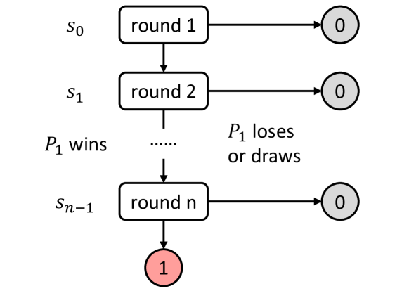
Figure 1: Illustration of the $RPS(n)$ game.

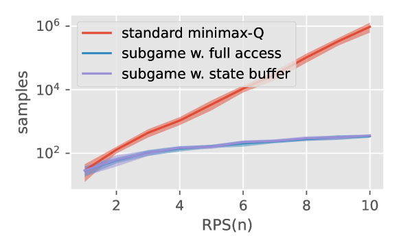
Figure 2: Number of samples used to learn the NE Q-values of $RPS(n)$ games.

In this section, we show by a simple illustrative example that vanilla MARL methods like minimax-Q require exponentially many samples to derive the NE. However, if we can dynamically set the initial state distribution and induce an appropriate order of subgames to learn, the sample complexity can be substantially reduced from exponential to linear. Such an observation motivates our proposed algorithm described in later sections.

Iterated Rock-Paper-Scissors Game

We introduce an iterated variant of the Rock-Paper-Scissor (RPS) game, denoted as $RPS(n)$. As shown in Fig. 1, $P_{1}$ and $P_{2}$ play the RPS game for up to $n$ rounds. If $P_{1}$ wins all rounds, it gets a reward of $1$ and $P_{2}$ gets a reward of $-1$. If $P_{1}$ loses or draws in any round, the game ends immediately without playing the remaining rounds and both players get zero rewards. Note that the $RPS(n)$ game is different from playing the RPS game repeatedly for $n$ times because players can play less than $n$ rounds and they only receive a non-zero reward if $P_{1}$ wins in all rounds. We use $s_{k}$ to denote the state where players have already played $k$ RPS games and are at the $k+1$ round. It is easy to verify that the NE policy for both players is to play Rock, Paper, or Scissors with equal probability at each state. Under this joint NE policy, $P_{1}$ can win one RPS game with $1/3$ probability, and the probability for $P_{1}$ to win all $n$ rounds and get a non-zero reward is $1/3^{n}$.

Consider using standard minimax-Q learning to solve the $RPS(n)$ game. With Q-functions initialized to zero, we execute the exploration policy to collect samples and perform the update in Eq. (6). Note all state-actions pairs are required to be visited to guarantee convergence to the NE. Therefore, in this sparse-reward game, random exploration will clearly take ${\mathcal{O}}(3^{n})$ steps to get a non-zero reward. Moreover, even if the exploration policy is perfectly set to the NE policy, the probability for $P_{1}$ to get the non-zero reward by winning all RPS games is still $\mathcal{O}(1/3^{n})$, requiring at least $\mathcal{O}(3^{n})$ samples to learn the NE Q-values of the $RPS(n)$ game.

Input: state sampler $\mathrm{oracle}(\cdot)$.

1 Initialize policy $\bm{\pi}$;

2 repeat

3       Sample $s^{0}$ $\sim\mathrm{oracle}(\mathcal{\mathcal{S}})$;

4       Rollout $\bm{\pi}$ in $\mathcal{MG}(s^{0})$;

5       Train $\bm{\pi}$ via MARL;

6      

7until $\bm{\pi}$ converges;

Output: final policy $\bm{\pi}$.

Algorithm 1 Subgame curriculum learning

From Exponential to Linear Complexity

An important observation is that the states in later rounds become exponentially rare in the samples generated by starting from the fixed initial state. If we can directly reset the game to these states and design a smart order of minimax-Q updates on the subgames induced by these states, the NE learning can be accelerated significantly. Note that $RPS(n)$ can be regarded as the composition of $n$ individual $RPS(1)$ games, a suitable order of learning would be from the easiest subgame $RPS(1)$ starting from state $s_{n-1}$ to the full game $RPS(n)$ starting from state $s_{0}$. Assuming we have full access to the state space, we first reset the game to $s_{n-1}$ and use minimax-Q to solve subgame $RPS(1)$ with $\mathcal{O}(1)$ samples. Given that the NE Q-values of $RPS(k)$ are learned, the next subgame $RPS(k+1)$ is equivalent to an $RPS(1)$ game where the winning reward is the value of state $s_{n-k}$. By sequentially applying minimax-Q to solve all $n$ subgames from $RPS(1)$ to $RPS(n)$, the number of samples required to learn the NE Q-values is reduced substantially from $\mathcal{O}(3^{n})$ to $\mathcal{O}(n)$.

In practice, we usually do not have access to the entire state space and cannot directly start from the last subgame $RPS(1)$. Instead, we can use a buffer to store all visited states and gradually span the state space. By resetting games to the newly visited states, the number of samples required to cover the full state space is still $\mathcal{O}(n)$, and we can then apply minimax-Q from $RPS(1)$ to $RPS(n)$. Therefore, the total number of samples is still $\mathcal{O}(n)$. We validate our analysis by running experiments on $RPS(n)$ games for $n=1,\cdots,10$ and the results averaged over ten seeds are shown in Fig. 2. It can be seen that the sample complexity reduces from exponential to linear by running minimax-Q over a smart order of subgames, and the result of using a state buffer in practice is comparable to the result with full access. The detailed analysis can be found in Appendix A.1.

Method

Algorithm 2 Subgame Automatic Curriculum Learning (SACL)

Input:

state buffers $\mathcal{M}$ with capacity $K$, probability $p$ to sample initial state from the state buffer.

1 Randomly initialize policy $\pi_{i}$ and value function $V_{i}$ for player $i=1,2$;

2 repeat

3       $V^{\prime}_{i}\leftarrow V_{i},\ i=1,2$;

       // Select subgame and train policy.

4       for each parallel environment do

5             Sample $s^{0}\sim\mathrm{sampler}(\mathcal{M})$ with probability $p$, else $s^{0}\sim\rho(\cdot)$;

6             Rollout in $\mathcal{MG}(s^{0})$ and collect samples;

7            

8      Train $\{\pi_{i},V_{i}\}_{i=1}^{2}$ via MARL;

       // Compute weight by Eq. (10) and update state buffer.

9       $\tilde{w}^{t}\leftarrow\alpha\cdot\mathbb{E}[\tilde{V}_{i}(s^{t})-\tilde{V}^{\prime}_{i}(s^{t})]^{2}+\mathrm{Var}(\{\tilde{V}_{i}(s^{t})\}_{i=1}^{2}),\\ \ t=0,\cdots,T$;

10       $\mathcal{M}\leftarrow\mathcal{M}\cup\{(s^{t},\tilde{w}^{t})\}_{t=0}^{T}$;

11       if $\|\mathcal{M}\|>K$ then

12             $\mathcal{M}\leftarrow\mathrm{FPS}(\mathcal{M},K)$;

13            

14      

15until $(\pi_{1},\pi_{2})$ converges;

Output: final policy $(\pi_{1},\pi_{2})$.

The motivating example suggests that NE learning can be largely accelerated by running MARL algorithms in a smart order over states. Inspired by this insight, we present a general framework to accelerate NE learning in zero-sum games by training over a curriculum of subgames. We further propose two practical techniques to instantiate the framework and present the overall algorithm.

Subgame Curriculum Learning

The key issue of the standard sample-and-update framework is that the rollout trajectories always start from the fixed initial state distribution $\rho$, so visiting states that are most critical for efficient learning can consume a large number of samples. To accelerate training, we can directly reset the environment to those critical states. Suppose we have an oracle state sampler $\textrm{oracle}(\cdot)$ that can initiate suitable states for the current policy to learn, i.e., generate appropriate induced subgames, we can derive a general-purpose framework in Alg. 1, which we call subgame curriculum learning. Note that this framework is compatible with any MARL algorithm for zero-sum Markov games.
A desirable feature of subgame curriculum learning is that it does not change the convergence property of the backbone MARL algorithm, as discussed below.

Proposition 1.

If all initial states $s^{0}$ with $\rho(s^{0})>0$ are sampled infinitely often, and the backbone MARL algorithm is guaranteed to converge to an NE in zero-sum Markov games, then subgame curriculum learning also produces an NE of the original Markov game.

The proof can be found in Appendix A.2. Note that such a requirement is easy to satisfy. For example, given any state sampler $\textrm{oracle}(\cdot)$, we can construct a valid mixed sampler by sampling from $\textrm{oracle}(\cdot)$ for probability $0<p<1$ and sampling from $\rho$ for probability $1-p$.

Remark. With a given state sampler, the only requirement of our subgame curriculum learning framework is that the environment can be reset to a desired state to generate the induced game. This is a standard assumption in the curriculum learning literature (Florensa et al. 2018; Matiisen et al. 2019; Portelas et al. 2020) and is feasible in many RL environments. For environments that do not support this feature, we can simply reimplement the reset function to make them compatible with our framework.

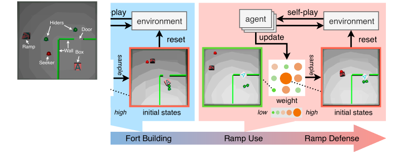
Figure 3: Illustration of SACL in the hide-and-seek environment. In the Fort Building stage, the states with hiders near the box have high weights (red) and agents can easily learn to build a fort by practicing on these subgames, while the states with randomly spawned hiders have low weights (green) and contribute less to learning.

Subgame Sampling Metric

A key question is how to instantiate the oracle sampler, i.e., which subgame should we train on for faster convergence? Intuitively, for a particular state $s$, if its value has converged to the NE value, that is, $V_{i}(s)=V_{i}^{*}(s)$, we should no longer train on the subgame induced by it. By contrast, if the gap between its current value and the NE value is substantial, we should probably train more on the induced subgame. Thus, a simple way is to use the squared difference of the current value and the NE value as the weight for a state and sample states with probabilities proportional to the weights. Concretely, the state weight can be written as

$$w(s) =\frac{1}{2}\sum_{i=1}^{2}(V_{i}^{*}(s)-V_{i}(s))^{2}$$ (7)

$$=\mathbb{E}_{i}\big{[}(V_{1}^{*}(s)-\tilde{V}_{i}(s))^{2}\big{]}$$ (8)

$$=\mathbb{E}_{i}\big{[}V_{1}^{*}(s)-\tilde{V}_{i}(s)\big{]}^{2}+\mathrm{Var}_{i}\big{[}V_{1}^{*}(s)-\tilde{V}_{i}(s)\big{]},$$ (9)

where $\tilde{V}_{1}(s)=V_{1}(s)$ and $\tilde{V}_{2}(s)=-V_{2}(s)$. The second equality holds because the game is zero-sum and $V_{2}^{*}(s)=-V_{1}^{*}(s)$. With random initialization and different training samples, $\{\tilde{V}_{i}\}_{i=1}^{2}$ can be regarded as an ensemble of two value functions, and the weight $w(s)$ becomes the expectation over the ensemble. The last equality further expands the expectation to a bias term and a variance term, and we sample state with probability $P(s)=w(s)/\sum_{s^{\prime}}w(s^{\prime})$. For the motivating example of $RPS(n)$ game, the NE value decreases exponentially from the last state $s_{n-1}$ to the initial state $s_{0}$. With value functions initialized close to zero, the prioritized subgames throughout training will move gradually from the last round to the first round, which is approximately the optimal order.

However, Eq. (9) is very hard to compute in practice because the NE value is generally unknown. Inspired by Eq. (9), we propose the following alternative state weight

$$\tilde{w}(s)=\alpha\cdot\mathbb{E}_{i}\big{[}\tilde{V}_{i}^{{\pi}_{i}^{(t)}}(s)-\tilde{V}^{{\pi}_{i}^{(t-1)}}_{i}(s)\big{]}^{2}+\mathrm{Var}_{i}\big{[}\tilde{V}_{i}(s)\big{]},$$ (10)

which takes a hyperparameter $\alpha$ and uses the difference between two consecutive value function checkpoints instead of the difference between the NE value and the current value in Eq. (9). The first term in Eq. (10) measures how fast the value functions change over time. If this term is large, the value functions are changing constantly and still far from the NE value; if this term is marginal, the value functions are probably close to the converged NE value. The second term in Eq. (10) measures the uncertainty of the current learned values and is the same as the variance term in Eq. (9) because $V^{*}_{1}(s)$ is a constant. If $\alpha=1$, Eq. (10) approximates Eq. (9) as $t$ increases. It is also possible to train an ensemble of value functions for each player to further improve the empirical performance. Additional analysis can be found in Appendix A.3.

Since Eq. (10) does not require the unknown NE value to compute, it can be used in practice as the weight for state sampling and can be implemented for most MARL algorithms. By selecting states with fast value change and high uncertainty, our framework prioritizes subgames where agents’ performance can quickly improve through learning.

Particle-based Subgame Sampler

With the sample weight at hand, we can generate subgames by sampling initial states from the state space. But it is impractical to sample from the entire space which is usually unavailable and can be exponentially large for complex games. Typical solutions include training a generative adversarial network (GAN) (Dendorfer, Osep, and Leal-Taixé 2020) or using a parametric Gaussian mixture model (GMM) (Portelas et al. 2020) to generate states for automatic curriculum learning. However, parametric models require a large number of samples to fit accurately and cannot adapt instantly to the ever-changing weight in our case. Moreover, the distribution of weights is highly multi-modal, which is hard to capture for many generative models.

We instead adopt a particle-based approach and maintain a large state buffer $\mathcal{M}$ using all visited states throughout training to approximate the state space. Since the size of the buffer is limited while the state space can be infinitely large, it is important to keep representative samples that are sufficiently far from each other to ensure good coverage of the state space. When the number of states exceeds the buffer’s capacity $K$, we use farthest point sampling (FPS) (Qi et al. 2017) which iteratively selects the farthest point from the current set of points. In our implementation, we first normalize each dimension of the states and the distance between two states is simply the Euclidean distance. More details can be found in Appendix B.1.

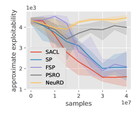
(a) MPE: exploitability.

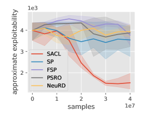
(b) MPE hard: exploitability.

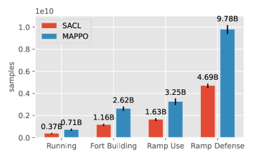
(c) HnS: number of samples.

Figure 4: Main experiment results in (a) MPE, (b) MPE hard, and (c) Hide-and-seek.

Scenario	SACL	SP	FSP	PSRO	NeuRD
pass and shoot	0.35 (0.13)	0.48 (0.31)	0.83 (0.10)	0.80 (0.09)	0.79 (0.15)
run pass and shoot	0.60 (0.04)	0.68 (0.09)	0.78 (0.08)	0.83 (0.04)	0.95 (0.04)
3 vs 1 with keeper	0.45 (0.06)	0.83 (0.03)	0.63 (0.25)	0.85 (0.05)	0.81 (0.16)

Table 1: Approximate exploitability of learned policies in different GRF scenarios.

Overall Algorithm

Combining the subgame sampling metric and the particle-based sampler, we present a realization of the subgame curriculum learning framework, i.e., the Subgame Automatic Curriculum Learning (SACL) algorithm, which is summarized in Alg. 2. When each episode resets, we use the particle-based sampler to generate suitable initial states $s_{0}$ for the current policy to learn. To satisfy the requirements in Proposition 1, we also reset the game according to the initial state distribution $\rho(\cdot)$ with $0.3$ probability. After collecting a number of samples, we train the policies and value functions using MARL. The weights for the newly collected states are computed according to Eq. (10) and used to update the state buffer $\mathcal{M}$. If the capacity of the state buffer is exceeded, we use FPS to select representative states-weight pairs and delete the others. An overview of SACL in the hide-and-seek game is illustrated in Fig. 3.

Experiment

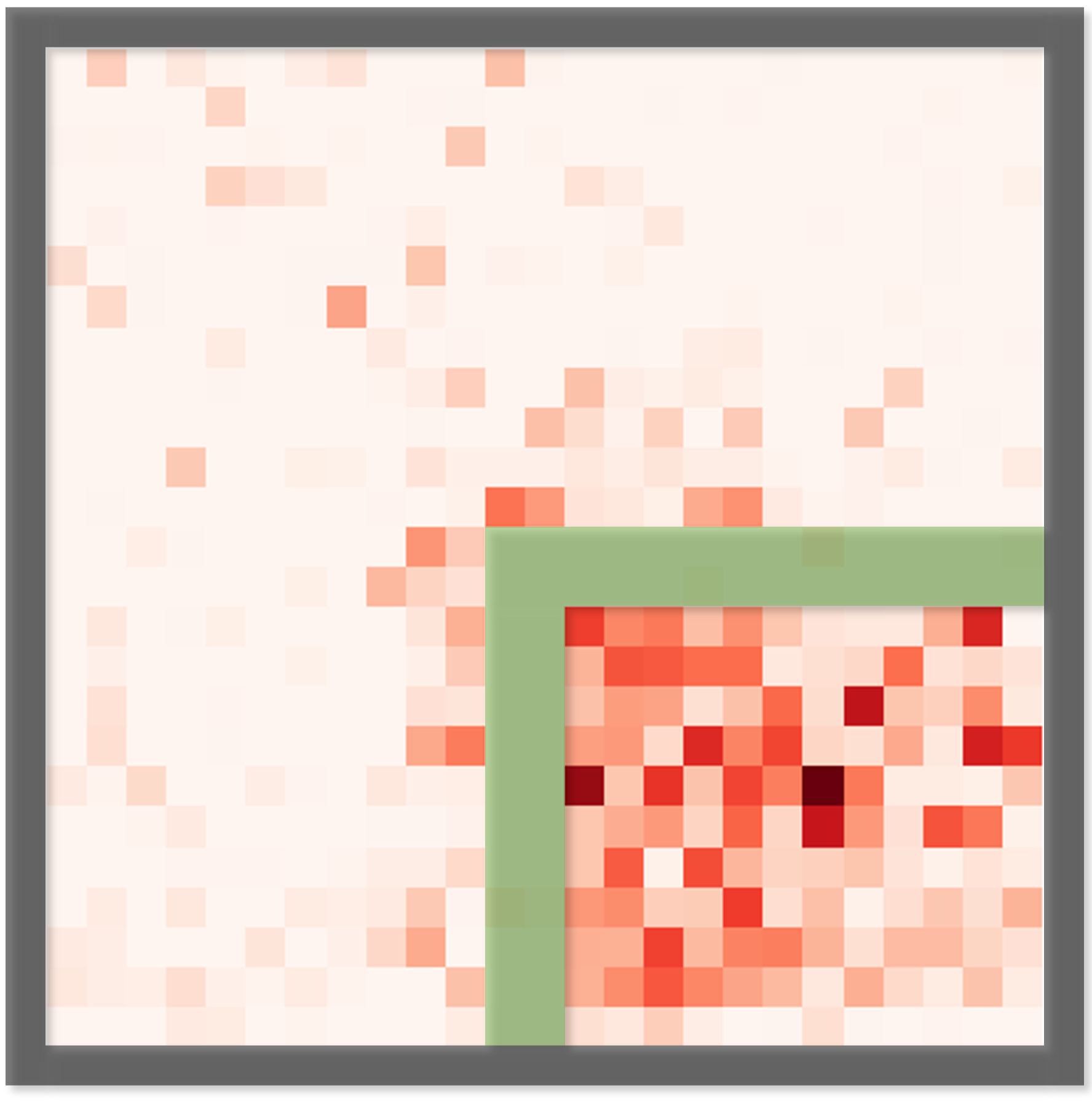
(a) Fort Building.

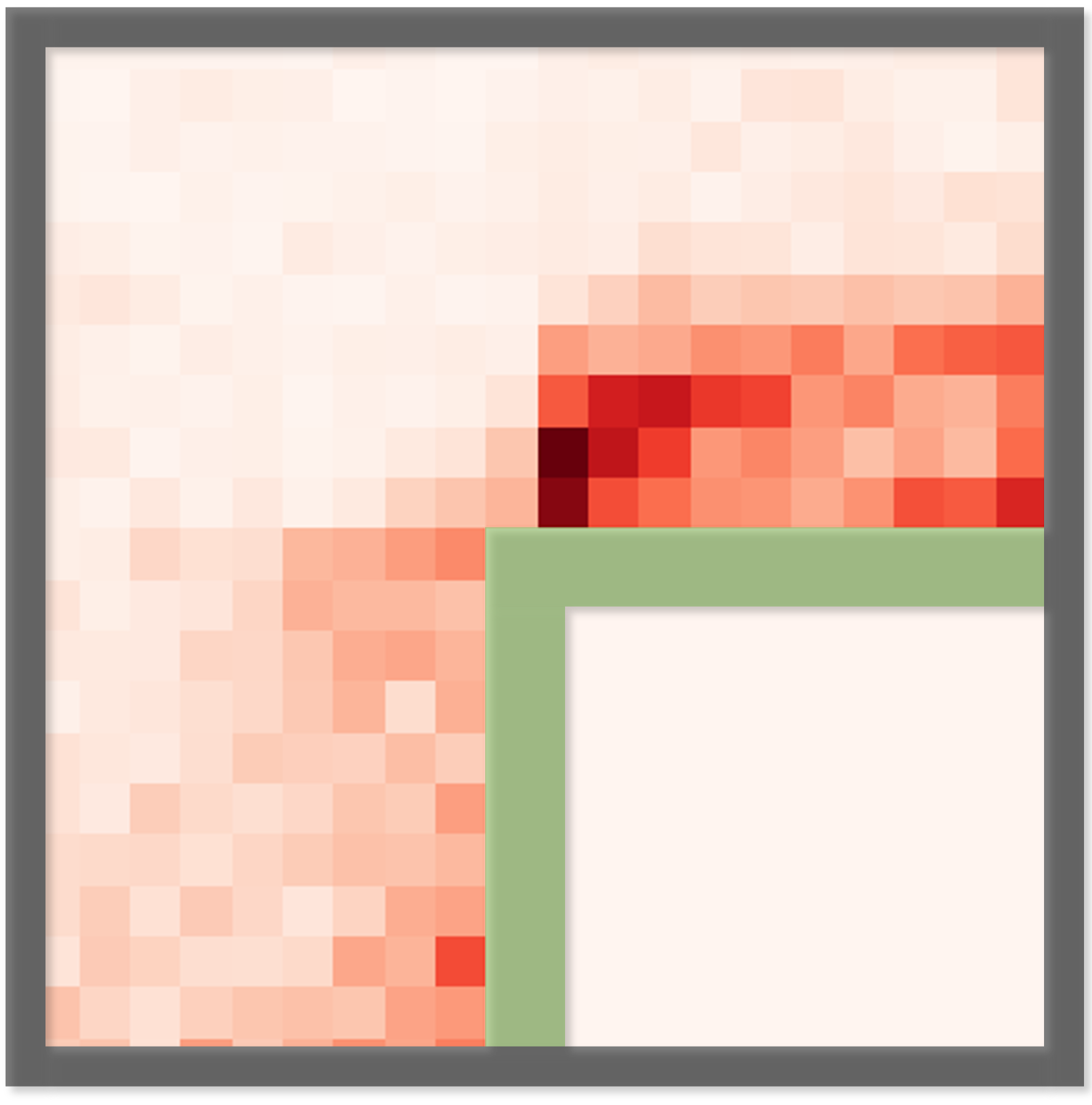
(b) Ramp Use.

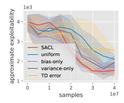
(c) Ablation on metric.

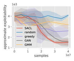
(d) Ablation on generator.

Figure 5: Visualization of the state distributions in HnS (a-b) and ablation studies (c-d).

We evaluate SACL in three different zero-sum environments: Multi-Agent Particle Environment (MPE) (Lowe et al. 2017), Google Research Football (GRF) (Kurach et al. 2020), and the hide-and-seek (HnS) environment (Baker et al. 2020). We use a state-of-the-art MARL algorithm MAPPO (Yu et al. 2021) as the backbone in all experiments. We evaluate the performance of policies by exploitability. How to define and compute the exploitability can be found in Appendix B.3.

Main Results

We first compare the performance of SACL in three environments against the following baselines for solving zero-sum games: self-play (SP), two popular variants including Fictitious Self-Play (FSP) (Heinrich, Lanctot, and Silver 2015) and Neural replicator dynamics (NeuRD) (Hennes et al. 2020), and a population-based training method policy-space response oracles (PSRO) (Lanctot et al. 2017). More implementation details can be found in Appendix B.2.

Multi-Agent Particle Environment. We consider the predator-prey scenario in MPE, where three slower cooperating predators chase one faster prey in a square space with two obstacles. In the default setting, all agents are spawned uniformly in the square. We also consider a harder setting where the predators are spawned in the top-right corner and the prey is spawned in the bottom-left corner. All algorithms are trained for 40M environment samples and the curves of approximate exploitability w.r.t. sample over three seeds are shown in Fig. 4(a) and 4(b). SACL converges faster and achieves lower exploitability than all baselines in both settings, and its advantage is more obvious in the hard scenario. This is because the initial state distribution in corners makes the full game challenging to solve, while SACL generates an adaptive state distribution and learns on increasingly harder subgames to accelerate NE learning. More results and discussions can be found in Appendix C.1.

Google Research Football. We evaluate SACL in three GRF academy scenarios, namely pass and shoot, run pass and shoot, and 3 vs 1 with keeper. In all scenarios, the left team’s agents cooperate to score a goal and the right team’s agents try to defend them. The first scenario is trained for 300M environment samples and the last two scenarios are trained for 400M samples. Table 1 lists the approximate exploitabilities of different methods’ policies over three seeds, and SACL achieves the lowest exploitability. Additional cross-play results and discussions can be found in Appendix C.2.

Hide-and-seek environment. HnS is a challenging zero-sum game with known NE policies, which makes it possible for us to directly evaluate the number of samples used for NE convergence. We consider the quadrant scenario where there is a room with a door in the lower right corner. Two hiders, one box, and one ramp are spawned uniformly in the environment, and one seeker is spawned uniformly outside the room. Both the box and the ramp can be moved and locked by agents. The hiders aim to avoid the lines of sight from the seeker while the seeker aims to find the hiders.

There is a total of four stages of emergent stages in HnS, i.e., Running and Chasing, Fort Building, Ramp Use, and Ramp Defense. As shown in Fig. 4(c), SACL with MAPPO backbone produces all four stages and converges to the NE policy with only 50% the samples of MAPPO with self-play. We also visualize the initial state distribution to show how SACL selects appropriate subgames for agents to learn. Fig. 5(a) depicts the distribution of hiders’ position in the Fort Building stage. The probabilities of states with hiders inside the room are much higher than states with hiders outside, making it easier for hiders to learn to build a fort with the box. Similarly, the distribution of the seeker’s position in the Ramp Use stage is shown in Fig. 5(b), and the most sampled subgames start from states where the seeker is close to the walls and is likely to use the ramp.

Ablation Study

We perform ablation studies to examine the effectiveness of the proposed sampling metric and particle-based sampler. All experiments are done in the hard predator-prey scenario of MPE and the results are averaged over three seeds. More ablation studies on state buffer size, subgame sample probability, and other hyperparameters can be found in Appendix C.1.

Subgame sampling metric. The sampling metric used in SACL follows Eq. (10) which consists of a bias term and a variance term. We compare it with five other metrics including a uniform metric, a bias-only metric, a variance-only metric and a temporal difference (TD) error metric. The last metric uses the TD error $|\delta_{t}|=|r^{t}+\gamma V(s^{t+1})-V(s^{t})|$ as the weight, which can be regarded as an estimation of value uncertainty. The results are shown in Fig. 5(c) and the sampling metric used by SACL outperforms both the bias-only metric and variance-only metric.

State generator. We substitute the particle-based sampler with other state generators including using GAN from the work (Dendorfer, Osep, and Leal-Taixé 2020) and using GMM from the work (Portelas et al. 2020). We also replace the FPS buffer update method with a uniform one that randomly keeps states and a greedy one that keeps states with the highest weights. Results in Fig. 5(c) show that our particle-based sampler with FPS update leads to the fastest convergence and lowest exploitability.

Related Work

A large number of works achieve faster convergence in zero-sum games by playing against an increasingly stronger policy. The most popular methods are self-play and its variants (Heinrich and Silver 2016; Bai, Jin, and Yu 2020; Jin et al. 2021; Perolat et al. 2022). Self-play creates a natural curriculum and leads to emergent complex skills and behaviors (Bansal et al. 2018; Baker et al. 2020). Population-based training like double oracle (McMahan, Gordon, and Blum 2003) and policy-space response oracles (PSRO) (Lanctot et al. 2017) extend self-play by training a pool of policies. Some follow-up works further accelerate training by constructing a smart mixing strategy over the policy pool according to the policy landscape (Balduzzi et al. 2019; Perez-Nieves et al. 2021; Liu et al. 2021; Feng et al. 2021). (McAleer et al. 2021) extends PSRO to extensive-form games by building policy mixtures at all states rather than only the initial states, but it still directly solves the full game starting from some fixed states.

In addition to policy-level curriculum learning methods, other works to accelerate training in zero-sum games usually adopt heuristics and domain knowledge like the number of agents (Long et al. 2020; Wang et al. 2020b) or environment specifications (Berner et al. 2019; Serrino et al. 2019; Tang et al. 2021). By contrast, our method automatically generates a curriculum over subgames without domain knowledge and only requires the environments can be reset to desired states. Subgame-solving technique (Brown and Sandholm 2017) is also used in online strategy refinement to improve the blueprint strategy of a simplified abstract game. Another closely related work to our method is (Chen et al. 2021b) which combines backward induction with policy learning, but this method requires knowledge of the game topology and can only be applied to finite-horizon Markov games.

Besides zero-sum games, curriculum learning is also studied in cooperative settings. The problem is often formalized as goal-conditioned RL where the agents need to reach a specific goal in each episode. Curriculum learning methods design or train a smart sampler to generate proper task configurations or goals that are most suitable for training advances w.r.t. some progression metric (Chen et al. 2016; Florensa et al. 2017, 2018; Racaniere et al. 2019; Matiisen et al. 2019; Portelas et al. 2020; Dendorfer, Osep, and Leal-Taixé 2020). Such a metric typically relies on an explicit signal, such as the goal-reaching reward, success rates, or the expected value of the testing tasks. However, in the setting of zero-sum games, these explicit progression metrics become no longer valid since the value associated with a Nash equilibrium can be arbitrary. A possible implicit metric is value disagreement (Zhang, Abbeel, and Pinto 2020) used in goal-reaching tasks, which can be regarded as the variance term in our metric. By adding a bias term, our metric approximates the squared distance to NE values and gives better results in ablation studies.

Our work adopts a non-parametric subgame sampler which is fast to learn and naturally multi-modal, instead of training an expensive deep generative model like GAN (Florensa et al. 2018). Such an idea has been recently popularized in the literature. Some representative samplers are Gaussian mixture model (Warde-Farley et al. 2019), Stein variational inference (Chen et al. 2021a), Gaussian process (Mehta et al. 2020), or simply evolutionary computation (Wang et al. 2019, 2020a). Technically, our method is related to prioritized experience replay (Schaul et al. 2015; Florensa et al. 2017; Li et al. 2022) with the difference that we maintain a buffer (Warde-Farley et al. 2019) to approximate the uniform distribution over the state space. Our method is also related to episodic memory replay (Blundell et al. 2016; Pritzel et al. 2017) which stores past experience and chooses actions based on previous success when similar states are encountered. By contrast, our method proactively resets the environment to intermediate states and collects experience in the sampled subgame.

Conclusion

We present SACL, a general algorithm for accelerating MARL training in zero-sum Markov games based on the subgame curriculum learning framework. We propose to use the approximate squared distance to NE values as the sampling metric and use a particle-based sampler for subgame generation. Instead of starting from the fixed initial states, RL agents trained with SACL can practice more on subgames that are most suitable for the current policy to learn, thus boosting training efficiency. We report appealing experiment results that SACL efficiently discovers all emergent strategies in the challenging hide-and-seek environment and uses only half the samples of MAPPO with self-play. We hope SACL can be helpful to speed up prototype development and help make MARL training on complex zero-sum games more affordable to the community.

A Analysis and Proofs

A.1 Detailed Analysis of the Motivating Example

We first show that the entire state space of $RPS(n)$ can be covered within $\mathcal{O}(n)$ samples by using a state buffer and resetting games to the newly visited states. We start with an empty state buffer, and the game resets according to its initial state distribution $\rho(\cdot)$, which always resets the game to $s_{0}$. With a random exploration policy, the probability for the game to transit from $s_{0}$ to $s_{1}$ is $1/3$. Therefore, the number of samples required to visit state $s_{1}$ in expectation is $\mathbb{E}[n(s_{1})]=3$. After $s_{1}$ is visited, this new state will be stored in the state buffer. Since we select the newly visited states as the initial state, the game will be reset to state $s_{1}$, and the additional number of samples required to visit state $s_{2}$ in expectation is also $\mathbb{E}[n(s_{2})]=3$. In general, by starting from state $s_{k-1}$, the expected number of samples to visit state $s_{k}$ is $\mathbb{E}[n(s_{k})]=3$, $k=1,2,\cdots,n-1$. Therefore, the total number of samples required to cover the whole state space is $\sum_{k=1}^{n-1}\mathbb{E}[n(s_{k})]=3(n-1)$, which is $\mathcal{O}(n)$.

Given that the state buffer has covered the entire state space, we then show that the NE Q-value of $RPS(n)$ can be learned by solving subgames with minimax-Q backward from $RSP(1)$ to $RPS(n)$. Consider using minimax-Q to solve $RPS(1)$, we can set the learning rate $\alpha=1$ since the transition is deterministic, and the NE Q-value of a state-action pair $(s,\bm{a})$ can be learned when this pair is in the collected samples. Therefore, to learn the NE Q-values of $RPS(1)$, we have to collect all state-action pairs at least one time. With a random exploration policy, the number of samples required to cover all state-action pairs is $\sum_{i=1}^{9}9/i=25.46<26$. Therefore, the NE Q-values of $RPS(1)$ can be learned within $26$ samples in expectation. Given that the NE Q-values of $RPS(k)$ are learned, the NE Q-values of $RPS(k+1)$ are only wrong at the first state and can be learned within $26$ episodes in expectation. Note that the expected episode length of $RPS(\infty)$ is $1.5$, so the expected episode length of $RPS(k)$ is less than $1.5$. Consider the episode used to learn the NE Q-values of the first state of $RPS(k+1)$, either $P_{1}$ wins and the expected episode length is less than $1+1.5=2.5$, or $P_{1}$ draws or loses and the episode length is $1$. In both cases, the episode length is less than $2.5$, so the number of samples used is less than $26*2.5=65$. Therefore, the total number of samples used to learn the NE Q-values from $RPS(1)$ to $RPS(n)$ is less than $65(n-1)$, which is $\mathcal{O}(n)$.

Since it takes $\mathcal{O}(n)$ samples to cover the entire state space and $\mathcal{O}(n)$ samples to learn the NE Q-values from $RPS(1)$ to $RPS(n)$, the total number of samples is still $\mathcal{O}(n)$.

A.2 Proof of Proposition 1

See 1

Proof.

When the policy trained by subgame curriculum learning converges, it is an NE of all subgames induced by the proposed states, including all initial states $s_{0}$ with $\rho(s_{0})>0$. Therefore, it is an NE of the original Markov game. ∎

A.3 Detailed Analysis of the State Sampling Metric

We approximate the squared difference between the current value and the NE value by Eq. (10), i.e.

$$w(s) =\mathbb{E}_{i}\big{[}(V_{1}^{*}(s)-\tilde{V}_{i}(s))^{2}\big{]}$$

$$\approx\alpha\cdot\mathbb{E}_{i}\big{[}\tilde{V}_{i}^{(t)}(s)-\tilde{V}^{(t-1)}_{i}(s)\big{]}^{2}+\mathrm{Var}_{i}\big{[}\tilde{V}_{i}(s)\big{]}.$$

The first term in Eq. (10) uses a hyperparameter $\alpha$ and the difference between two consecutive value function checkpoints to estimate the difference between the current value and the NE value. As shown in Fig. 6, when the value function changes monotonically throughout training, the estimate can be regarded as a first-order approximation of the bias term. However, the value function of zero-sum games may oscillate up and down in different emergent stages (like in hide-and-seek), as shown in Fig. 7. In this case, the difference between two value function checkpoints is no longer an approximation of the distance to the NE value but a first-order approximation of the difference between the current value and the next local minimal or local maximal value $V_{1}^{(*,k)}$, and the weight becomes the approximated squared difference between the current value and the next local optimal value, i.e.,

$$w(s) =\alpha\cdot\mathbb{E}_{i}\big{[}\tilde{V}_{i}^{(t)}(s)-\tilde{V}^{(t-1)}_{i}(s)\big{]}^{2}+\mathrm{Var}_{i}\big{[}\tilde{V}_{i}(s)\big{]}$$

$$\approx\mathbb{E}_{i}\big{[}V_{1}^{(*,k)}(s)-\tilde{V}_{i}(s)\big{]}^{2}+\mathrm{Var}_{i}\big{[}V_{1}^{(*,k)}(s)-\tilde{V}_{i}(s)\big{]}$$

$$=\mathbb{E}_{i}\big{[}(V_{1}^{(*,k)}(s)-\tilde{V}_{i}(s))^{2}\big{]}.$$ (11)

Therefore, by using the weight in Eq. (10), we are not directly prioritizing states where the values are far from the NE values but prioritizing states where the values are far from the next local optimal value. For example, in Fig. 7, before the value function has learned the first local maximal value $V_{1}^{(*,1)}$, we will give larger weights to states that are far from the $V_{1}^{(*,1)}$ to accelerate the first stage of learning $V_{1}^{(*,1)}$. After $V_{1}^{(*,1)}$ is successfully learned, we will then prioritize states that are far from the second local optimal value $V_{2}^{(*,1)}$ and accelerate the second stage of learning $V_{1}^{(*,2)}$. Finally, we learn towards the NE value $V_{1}^{(*,3)}=V_{1}^{*}$. By accelerating the learning in each stage, we make the NE learning process more efficient in total.

It is also possible to train an ensemble of value functions for each player to improve the estimation. Suppose we train $M$ value functions for player $i$ and denote them as $\{\tilde{V}_{i,m}\}_{m=1}^{M}$ for $i=1,2$, then the weight for state $s$ becomes

$$w(s) =\alpha\cdot\mathbb{E}_{i,m}\big{[}\tilde{V}_{i,m}^{(t)}(s)-\tilde{V}^{(t-1)}_{i,m}(s)\big{]}^{2}+\mathrm{Var}_{i,m}\big{[}\tilde{V}_{i,m}(s)\big{]},$$ (12)

where the expectation and variance are taken over both the player index $i$ and the ensemble index $m$.

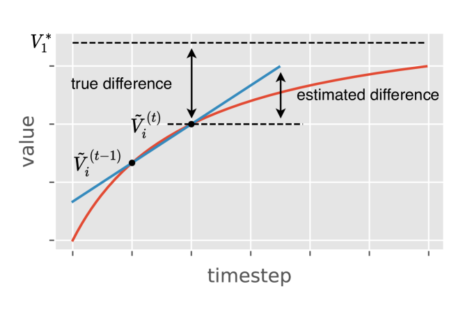
Figure 6: Approximation of the bias term when value function changes monotonically.

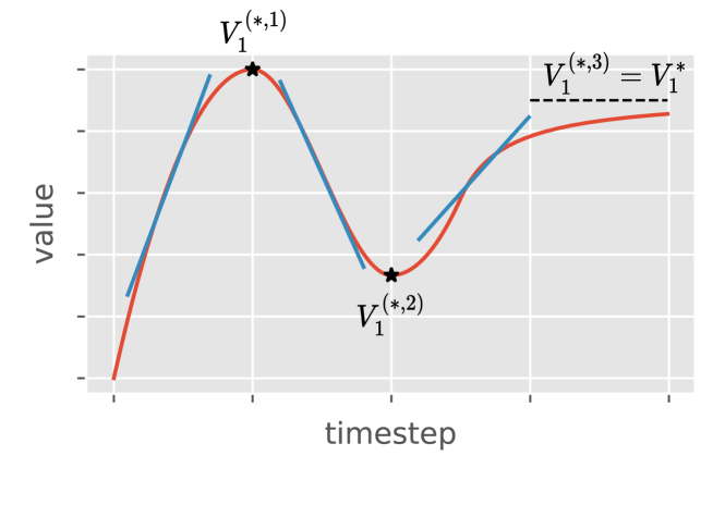
Figure 7: Approximation in different stages when value function oscillates in training.

A.4 Difference of SACL and subgame solving method for extensive-form games

First, we would like to emphasize that the goal of this work is to accelerate learning in complex fully-observable Markov games. In our experiments, the learning agents do not know the transition of the games, following the standard assumption in reinforcement learning.

For extensive-form games, such as poker, there has been extensive literature on how to construct and solve a subgame (Zhang and Sandholm 2021) (Brown and Sandholm 2017) (Burch et al. 2014) (Moravcik et al. 2016). The idea of subgame solving is first to get a blueprint strategy of the abstracted game and use it to play the original game. As the game progresses and the remaining game becomes tractable, the specific subgame is solved in real-time to create a combined final policy. Subgame solving typically uses iterative updates based on regret matching to find the policy, which requires the traverse of the game tree.

B Implementation Details

B.1 Implementation of Farthest Point Sampling

In the subgame sampler, we use a state buffer to approximate the whole state space and record the state weights. In principle, the states in the buffer should span the entire state space and distribute uniformly, but the rollout data is usually concentrated and very similar to each other. Therefore, we need to select states that are sufficiently far from each other to ensure good coverage of the state space. Formally, we need to select a subset $S^{\prime}$ of size $K$ from the whole set $S$ so that the sum of the shortest distances between states in the subset $S^{\prime}$ is maximized, i.e., $max_{S^{\prime}\subset S,|S^{\prime}|=K}\Sigma_{s\in S^{\prime}}min_{s^{\prime}\in S^{\prime}}|s-s^{\prime}|$. The farthest point sampling is a greedy algorithm that efficiently finds an approximate optimal solution to this problem.

In general, FPS iteratively selects the farthest point from the current set of points. The distance between two states is simply the Euclidean distance. The distance between a state $s_{a}$ and a set of states $S$ is the smallest distance between $s_{a}$ and any state in $S$, i.e., $min_{s\in S}|s_{a}-s|$. For implementation, we first normalize each dimension of the state vector to make all values lie in the range $[0,1]$. Then, we directly use the farthest_point_sampler() function from the Deep Gragh Library to utilize GPUs for fast and stable results.

B.2 Training Details

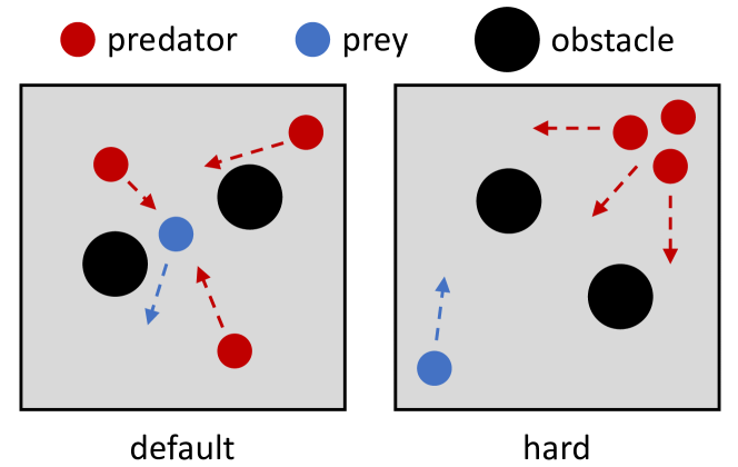
Figure 8: Illustration of the default and hard setting of predator-prey in MPE.

Multi-Agent Particle Environment. The default and hard settings of the predator-prey scenario in MPE are shown in Fig. 8. The environment is a 2D square space, and the length of a side is 4, i.e., $\{(x,y)|-2\leq x\leq 2,-2\leq y\leq 2\}$. Three predators (red) cooperatively chase one prey (blue), and there are two obstacles in the space. In the default setting, all agents and obstacles are randomly spawned. In the hard setting, predators are uniformly spawned in the top-right corner, i.e., $\{(x,y)|1\leq x\leq 2,1\leq y\leq 2\}$, the prey is spawned in the bottom-left corner, i.e., $\{(x,y)|-2\leq x\leq-1,-2\leq y\leq-1\}$, and the obstacles are still randomly generated in the square.

This environment is fully observable, and the state of each agent is a concatenation of the positions and the velocities of all agents and the positions of all obstacles. The action space is discrete with $5$ actions: idle, up, down, left, right. The environment lasts for $200$ steps. In each step, if any predator collides with the prey, all predators get a reward of $+1$, and the prey gets a reward of $-1$.

The actor and critic networks use the transformer architecture. The inputs first pass through a LayerNorm layer. The normalized states are divided into different entities, including self, other agents, obstacles, and time; then, each entity passes through fully connected layers to get its embedding. The weights of the embedding layers are shared within entities of the same type. Then, the embedding of each entity is concatenated with the self-states and passed through a self-attention network. Then, we average the output of the attention block and concatenate it with the self-embedding to get the final representation. This representation is then passed through a LayerNorm layer and an MLP layer and then produces the value through a critic’s head and the action through an actor’s head. All hyperparameters for training are listed in Table 2.

Hyperparameters	Value
Learning rate	5e-4
Discount rate ($\gamma$)	0.99
GAE parameter ($\lambda_{\textrm{GAE}}$)	0.95
Gradient clipping	10.0
Adam stepsize	1e-5
Value loss coefficient	1
Entropy coefficient	0.01
Parallel threads	100
PPO clipping	0.2
PPO epochs	5
Size of embedding layer	32
Size of MLP layer	64
Size of LSTM layer	64
Residual attention layer	8
probability $p$	0.7
Ensemble size $M$	3
Capacity $K$	10000
Weight of the value difference $\alpha$	0.7

Table 2: Hyperparameters of MPE.

Hyperparameters	Value
Learning rate	5e-4
Discount rate ($\gamma$)	0.99
GAE parameter ($\lambda_{\textrm{GAE}}$)	0.95
Gradient clipping	10.0
Adam stepsize	1e-5
Value loss coefficient	1
Entropy coefficient	0.01
Parallel threads	200
PPO clipping	0.2
PPO epochs	10
Size of MLP layer	64
probability $p$	0.7
Ensemble size $M$	3
Capacity $K$	10000
Weight of the value difference $\alpha$	0.7

Table 3: Hyperparameters of GRF.

Length	Information
22	(x,y) coordinates of left team players
22	(x,y) direction of left team players
22	(x,y) coordinates of right team players
22	(x,y) direction of right team players
3	(x, y and z) ball position
3	ball direction
3	one hot encoding of ball ownership (none, left, right)
11	one hot encoding of which player is active
7	one hot encoding of game mode

Table 4: Information in the state vector of GRF.

Hyper-parameters	Value
Learning rate	3e-4
Discount rate ($\gamma$)	0.998
GAE parameter ($\lambda_{\textrm{GAE}}$)	0.95
Gradient clipping	5.0
Adam stepsize	1e-5
Value loss coefficient	1
Entropy coefficient	0.01
PPO clipping	0.2
Chunk length	10
PPO epochs	4
Horizon	80
Mini-batch size	64000
Size of embedding layer	128
Size of MLP layer	256
Size of LSTM layer	256
Residual attention layer	32
Weight decay coefficient	$10^{-6}$
probability $p$	0.7
Ensemble size $M$	3
Capacity $K$	10000
Weight of the value difference $\alpha$	1.0

Table 5: Hyperparameters of HnS.

Hyperparameters	Value
Learning rate	5e-4
Discount rate ($\gamma$)	0.99
GAE parameter ($\lambda_{\textrm{GAE}}$)	0.95
Gradient clipping	20.0
Adam stepsize	1e-5
Value loss coefficient	1
Entropy coefficient	0.01
PPO clipping	0.2
chunk length	10
PPO epochs	15
Horizon	60
Parallel threads	300
probability $p$	0.7
Ensemble size $M$	3
Capacity $K$	2000

Table 6: Hyperparameters of the cooperative task in HnS

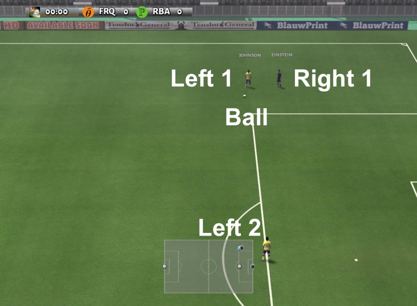
Figure 9: Pass and shoot scenario in GRF.

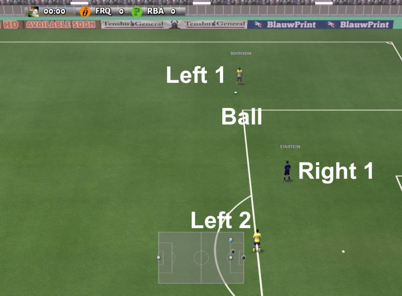
Figure 10: Run, pass and shoot scenario in GRF.

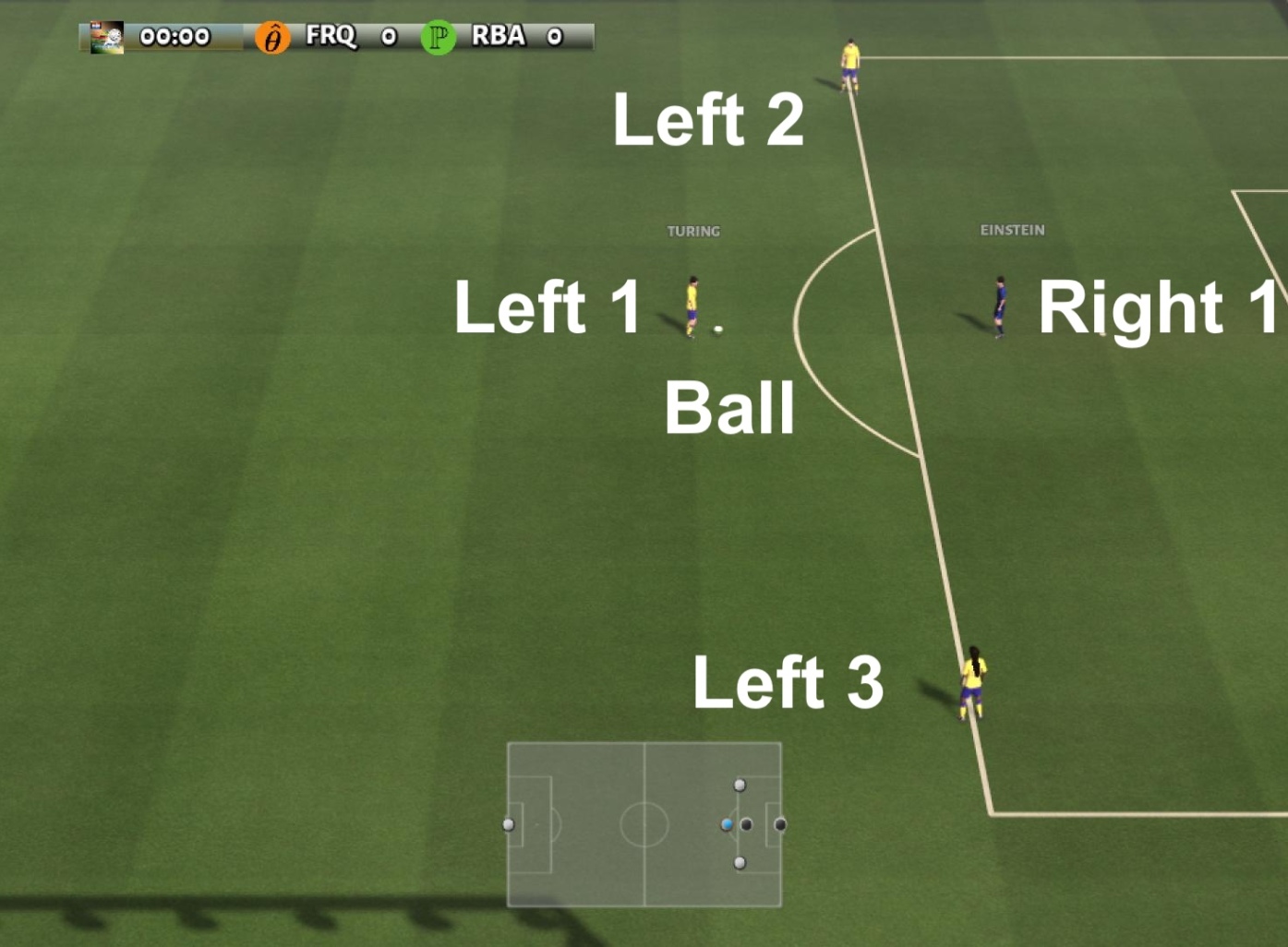
Figure 11: 3 vs 1 with keeper scenario in GRF.

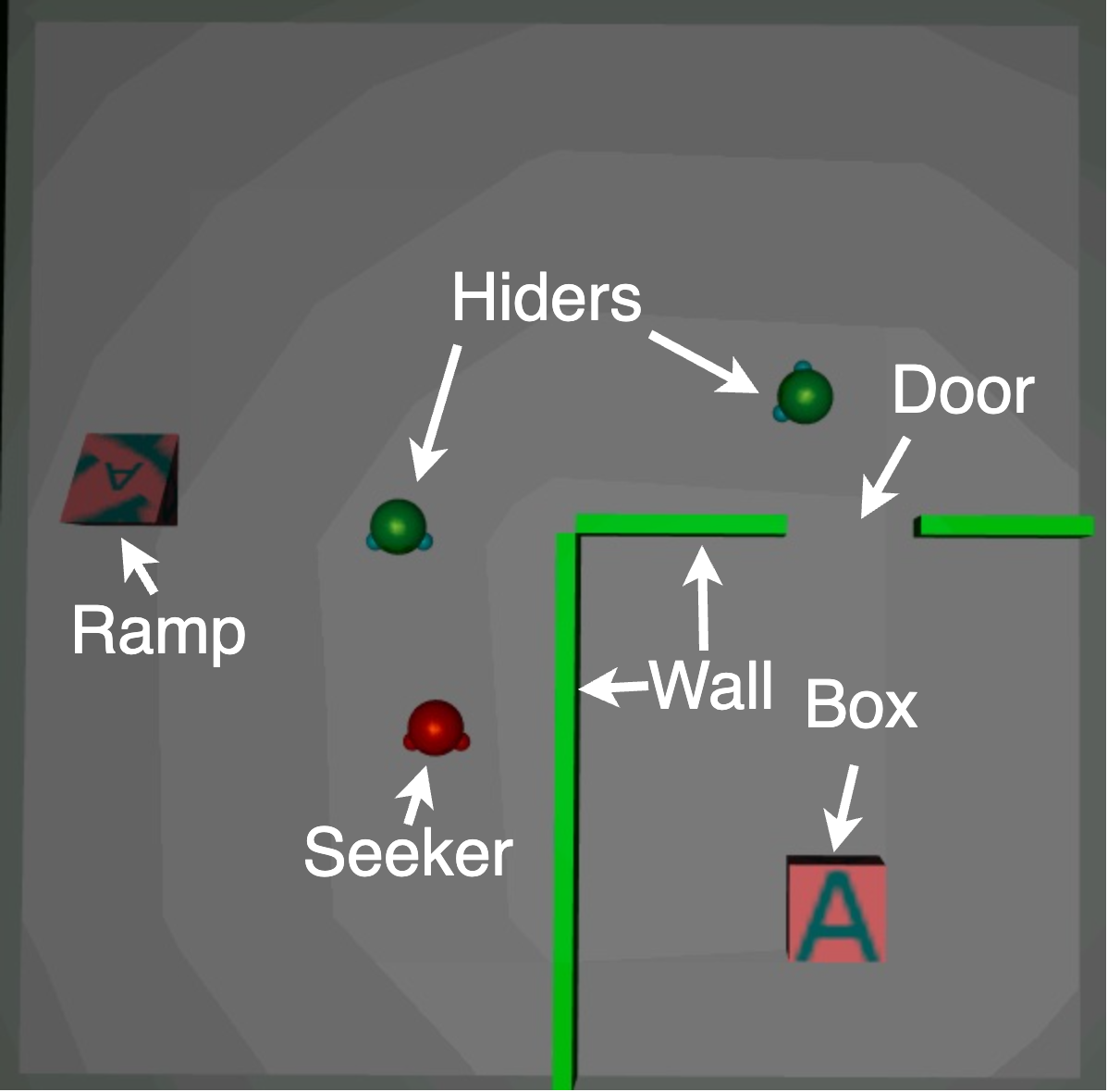
Figure 12: Quadrant scenario in HnS.

Google Research Football. The environment is a physics-based 3D football simulation, and the length and width are 2.0 and 0.9, i.e., $\{(x,y)|-1.0\leq x\leq 1.0,-0.45\leq y\leq 0.45\}$. The pass and shoot scenario in GRF is shown in Fig. 12. There are five players and a soccer ball in the environment, with a scripted goalkeeper and two RL attackers on the left side and a scripted goalkeeper and one RL defender on the right side. The left goalkeeper is spawned at $(-1.0,0.0)$ and the two attackers are spawned at $(0.7,0.0)$ and $(0.7,-0.3)$. The right goalkeeper is spawned at $(1.0,0.0)$ and the defender is spawned at $(0.75,-0.3)$. The ball is spawned at $(0.7,-0.28)$. The run, pass and shoot scenario in GRF is shown in Fig. 12. There are five players and a soccer ball in the environment, with a scripted goalkeeper and two RL attackers on the left side and a scripted goalkeeper and one RL defender on the right side. The left goalkeeper is spawned at $(-1.0,0.0)$ and the two attackers are spawned at $(0.7,0.0)$ and $(0.7,-0.3)$. The right goalkeeper is spawned at $(1.0,0.0)$ and the defender is spawned at $(0.75,-0.1)$. The ball is spawned at $(0.7,-0.28)$. The 3 vs 1 with keeper scenario in GRF is shown in Fig. 12. There are six players and a soccer ball in the environment, with a scripted goalkeeper and three RL attackers on the left side and a scripted goalkeeper and one RL defender on the right side. The left goalkeeper is spawned at $(-1.0,0.0)$ and the three attackers are spawned at $(0.6,0.0)$, $(0.7,0.2)$ and $(0.7,-0.2)$. The right goalkeeper is spawned at $(1.0,0.0)$ and the defender is spawned at $(0.75,0.0)$. The ball is spawned at $(0.6,0.0)$. In all three environments, attackers have to learn how to dribble the ball, cooperate with teammates to pass the ball, and overcome the defender’s defense to score goals.

The environment is fully observable, and the state of each agent is a 115-dimensional vector, including the coordinates of left team players, the directions of left team players, the coordinates of right team players, the directions of right team players, the ball position, the ball direction, one hot encoding of ball ownership, one hot encoding of which player is active and one hot encoding of game mode. The detailed information is listed in Table 4. The action space is discrete with 19 actions: idle, left, top left, top, top right, right, bottom right, bottom, bottom left, long pass, high pass, short pass, shoot, start sprinting, reset current movement direction, stop sprinting, slide, start dribbling and stop dribbling. An episode lasts a maximum of 200 steps. The environment ends prematurely when one side scores, the possession of the ball changes, or the game is out of play. We use the standard scoring and checkpoint rewards provided by the football engine. Specifically, if the left team scores a goal in each step, all left players get a reward of +1, and the right player gets -1. There are also ten concentric circles with the goal in the center, called checkpoint regions. The left team obtains an additional checkpoint reward of +0.1 when they possess the ball, and first move into the next checkpoint region, and the right team gets -0.1. Checkpoint rewards are only given once per episode.

The inputs of the actor and critic networks first pass through a LayerNorm layer. The normalized states then pass through an MLP layer and then produce the value through a critic head and the action through an actor’s head. All hyperparameters for training are listed in Table 3.

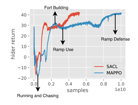
Figure 13: Checkpoints of four rounds of emergent strategies in HnS.

Hide-and-seek Environment.

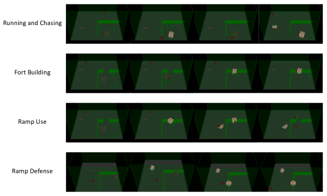
Figure 14: Sample trajectory traces from each emergent stage in quadrant scenario of HnS.

The quadrant scenario in the hide-and-seek environment is shown in Fig. 12. The environment is a square space with a square room with a door in the bottom-right corner. There are two hiders (green), one seeker (red), one box, and one ramp. At the beginning of each episode, the hiders, box, and ramp are uniformly spawned inside the room, and the seeker is uniformly spawned outside the room.

The environment is fully observable, and the state of each agent is a concatenation of the positions and velocities of all agents, the positions, velocities, and lock flags of the box and the ramp, and the current timestep. The action space is discrete, and agents can choose to move in 4 directions: grab and lock/unlock. Each episode lasts for $80$ steps and is divided into 2 phases: the preparation phase and the main phase. In the preparation phase, the seeker is fixed, and only the hiders can act to prepare for the main phase. No reward is given to any agent in the preparation phase. In the main phase, all agents can act, and the seeker tries to find the hiders, and the hiders try to avoid being discovered. When the seeker spots the hiders, the seeker gets a reward of $+1$ at this step, and the hiders get a reward of $-1$. Otherwise, the seeker gets a reward of $-1$, and the hiders get $+1$.

There are a total of 4 emergent stages in this game, as shown in Fig. 14. (1) Running and Chasing: The hiders learn to run away from the seeker to avoid detection, while the seeker learns to chase the hiders. The seeker is the winner at this stage, and the average episode reward of hiders is about $-20$. (2) Fort Building: In the preparation phase, the hiders learn to use the box to block the door and lock it in place to build a fort so that the seeker cannot enter the room and see the hider. The hiders are the winners in this stage, and the average episode reward of hiders is about $30$. (3) Ramp Use: The seeker learns to move the ramp to the wall of the room and use it to get into the room. The average episode reward of hiders reduces to about $25$ but is still larger than $0$. (4) Ramp Defense: In the preparation phase, the hiders learn to move the ramp into the room or push it far away from the wall and lock it to prevent being used by the seeker. The seeker can no longer enter the room and find the hiders. The average episode reward of hiders is about $40$ at this stage.

We adopt the same network architecture as (Baker et al. 2020). The states are divided into different entities, including self, other agents, box, and ramp; then, each entity passes through fully connected layers to get its embedding. The weights of the embedding layers are shared within entities of the same type. Then, the embedding of each entity is concatenated with the self embedding and passed through a self-attention network. Then, we average the output of the attention block and concatenate it with the self-embedding to get the final representation. This representation is then passed through an MLP layer and an LSTM layer and then produces the value through a critic head and the action through an actor’s head. All hyperparameters of HnS are listed in Table 5.

Besides zero-sum games, it is also possible to use SACL in cooperative tasks. We choose the Ramp Use stage in HnS to show that SACL can produce comparable results to curriculum learning algorithms specialized for cooperative tasks (Chen et al. 2021a). In this task, there is one hider with a fixed policy, one seeker to train, one box, and one ramp. We need to train a seeker policy to use the ramp to get into the quadrant room for positive rewards. The environment is fully observable, and the state is the same as that in the quadrant scenario. We use the same prior knowledge to define easy tasks as  (Chen et al. 2021a), which prioritizes states where the ramp is right next to the wall, and agents are next to the ramp. All hyperparameters are listed in Table 6.

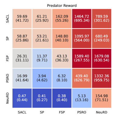
(a) MPE.

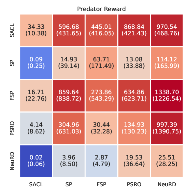
(b) MPE hard.

Figure 15: Cross-play results in MPE and MPE hard.

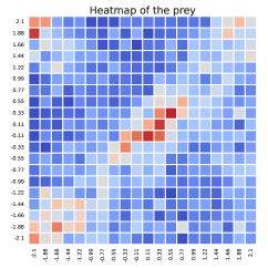
(a) 5M: Center.

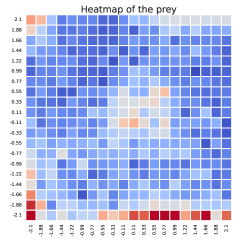
(b) 8M: Edges.

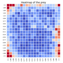
(c) 15M: Corners.

Figure 16: Visualization of the prey’s initial position heatmap generated by SACL at different training timesteps.

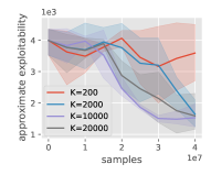
(a) Buffer size.

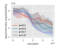
(b) Sample probability.

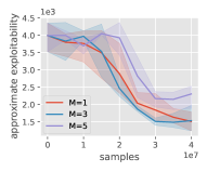
(c) Ensemble size.

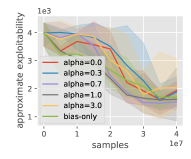
(d) Weight of value difference.

Figure 17: Ablation studies in MPE hard.

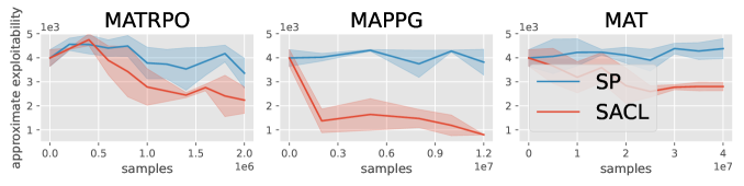
Figure 18: SACL outperforms self-play (SP) in all three MARL algorithms.

B.3 Evaluation Details

Exploitability.

In zero-sum games, because the performance of one player’s policy depends on the other player’s policy, the return curve throughout training is no longer a suitable evaluation method. One way to compare the performance of different policies is to use cross-play, which uses a tournament-style match between any two policies and records the results in a payoff matrix. However, due to the non-transitivity of many zero-sum games (Balduzzi et al. 2019), winning other policies does not necessarily mean being close to NE policies. Hence, a better way to evaluate the performance of policies is to use exploitability. Given a pair of policies $(\pi_{1},\pi_{2})$, the exploitability is defined as

$$\mathrm{exploitability}(\pi_{1},\pi_{2})=\sum_{i=1}^{2}\max_{\pi_{i}^{\prime}}\mathbb{E}\left[V_{i}^{(\pi_{i}^{\prime},\pi_{-i})}(s^{0})\right].$$ (13)

Exploitability can be roughly interpreted as the “distance” to the joint NE policy. In complex environments like the ones we use, the exact exploitability cannot be calculated because we cannot traverse the policy space to find $\pi_{i}^{\prime}$ that maximizes the value. We compute the approximate exploitability by training an approximate best response $\tilde{\pi}_{i}^{\prime}$ of the fixed policy $\pi_{i}$ using MAPPO. A BR is trained for 200M samples in MPE and 400M in GRF. The lower the exploitability, the better the algorithm. We use the checkpoints of an algorithm’s policy trained with different numbers of environment steps to estimate the exploitability. Specifically, we run SACL in MPE and save a policy checkpoint when the agent has consumed 0M, 5M, 10M, 15M, …, and 40M environment samples. Then, we keep each checkpoint fixed and train an adversarial policy to be the best response of the fixed policy to estimate the exploitability. Then, we get an exploitability curve of SACL over samples. Finally, we repeat this procedure for two more seeds, average the results, and plot the std error. For a single algorithm, we trained $9\times 3=27$ (checkpoints $\times$ seeds) best-response policies to plot one curve in the exploitability graph.

Cross-play. We evaluate SACL and other baselines by cross-play, which uses a head-to-head match between any two policies and records the results in a payoff matrix. In MPE, the element of the payoff matrix represents the episodic reward of the predators, and in GRF, it represents the win rate of the red team. More specifically, we train three seeds for each algorithm and match three models of one algorithm against the three models of the opponent algorithm, i.e., we get $3\times 3=9$ competitions between any two algorithms and report the average results and the std error. For example, in MPE, we use three different predators of SACL to compete with three different preys of SP to get the episode predator reward. We can evaluate the performance of the predator using the elements of a row and evaluate the performance of the prey using the elements of a column. We use the first row to represent the predator of SACL, then a larger value in this row than other rows means that the predator of SACL is better than other algorithms. We use the first column to represent the prey of SACL, then a smaller value in this column than in other columns means that the prey of SACL is better than other algorithms.

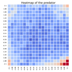
(a) FPS.

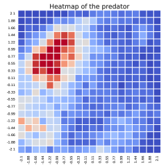
(b) Greedy.

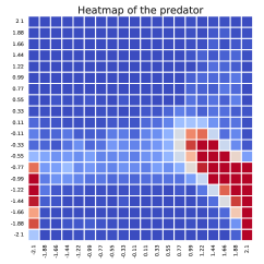
(c) Random.

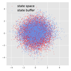
(d) FPS.

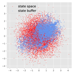
(e) Greedy.

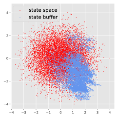
(f) Random.

Figure 19: Visualization of the state buffer and projection of tasks in the state buffer to 2-dimension by principal component analysis generated by three update methods.

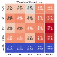
(a) Pass and shoot.

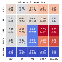
(b) Run, pass and shoot.

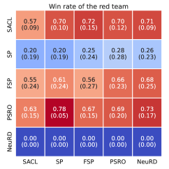
(c) 3 vs 1 with keeper.

Figure 20: Cross-play results in GRF.

Four rounds of emergent strategies in HnS. As shown in Fig. 13, we use three inflection points to evaluate the sample required to produce the first three stages. More specifically, the Running and Chasing phase ends when the hider’s reward decreases to the lowest value of about $-20$. When the hider’s reward begins to increase, the Fort-Building phase begins and continues until the hider’s reward reaches a local maximum of about $30$. Then, the agents move to the Ramp-Defense phase until the hider’s reward reaches a local minimum and begins the final Ramp-Use stage. We choose the point when the hider’s episode reward reaches $40$ as the end of the final stage.

C Additional Experiment Results

C.1 Multi-Agent Particle Environment

Cross-play. The results of cross-play at $40M$ in MPE and MPE hard are shown in Fig. 15(a) and Fig. 15(b). In MPE and MPE hard, the predator and prey of SACL beat all baselines. For example, let x be the row x and y represent the column y of the payoff matrix. We compare the predator of SACL with FSP using rows 1 and 3 and find that the elements of row 1 are larger than the elements of row 3, i.e., the predator of SACL is better than FSP. The elements of column 1 are smaller than the elements of column 3, which means the prey of SACL is better than FSP. The prey trained by SACL swerves to avoid the predators when the predators surround him, and the predators learn to capture the prey in the two environments. SP is comparable with SACL in MPE, but in the hard setting, SP does not converge to the NE policy due to the large initial distance between predator and prey. FSP also performs worse than SACL in the hard setting for the same reason as SP. For PSRO, it is even difficult to obtain the best response corresponding to the prey of random policy in MPE hard because the initial distance between prey and predator is too far. NeuRD performs poorly in both MPE and MPE hard because NeuRD’s update rules cause drastic policy changes and erratic convergence.

Visualization of subgame curriculum. To show the effectiveness of SACL, we visualize the change of the prey’s initial position heatmap produced by SACL in the MPE hard in Fig. 16 and find that it starts from the center and moves to the edges and corners which means that we train from easier subgames and gradually move to harder ones.

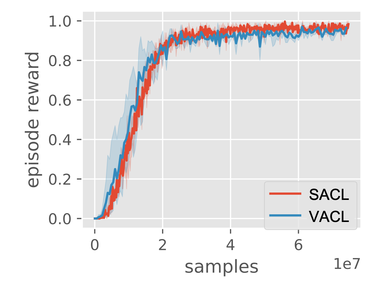
Figure 21: Seeker’s episode reward in the goal-reaching Ramp-Use task. SACL is comparable to a strong baseline VACL, which is specialized for goal-oriented problems.

Buffer size. As shown in Fig. 17(a), the buffer capacity $K$ must be large enough. When the buffer is too small, the states in the buffer cannot approximate the state space. When the buffer is too large, FPS consumes much time. So we finally choose $K=10000$.

Subgame sample probability. As shown in Fig. 17(b), we need more samples from the subgame buffer than uniform sampling in the training batch, and uniform sampling from the state space ensures global exploration. When $p$ is too small, SACL degenerates into SP, resulting in poor performance. When $p=1$, the lack of global exploration also leads to poor performance. Finally, we choose $p=0.7$.

Ensemble size. As shown in Fig. 17(c), we can train an ensemble of value functions for each player to improve the estimation. Excessive ensemble size requires much memory and training time. So we finally choose $M=3$.

Weight of value difference. As shown in Fig. 17(d), our algorithm is insensitive to the weight of the value difference $\alpha$. Empirically, we prefer $\alpha$ less than 1. We finally choose $\alpha=0.7$ in MPE, MPE hard, and GRF, $\alpha=1.0$ in Hns.

Different MARL backbones. We also conduct experiments in MPE hard with three more MARL algorithms including MAT (Wen et al. 2022), MATRPO, and MAPPG which are extensions of Trust Region Policy Optimization (TRPO) (Schulman et al. 2015) and Phasic Policy Gradient (PPG) (Cobbe et al. 2021) based on the centralized training and decentralized execution paradigm. The results in Fig. 18 show that SACL accelerates the learning process of all three algorithms.

Buffer update method. We further visualize the state distribution in the buffer generated by different update methods in Fig. 19. Fig. 19(a-c) shows the heatmaps of the predators’ position. Fig. 19(d-f) run PCA on the full state space and show the projection of the states in the buffer to the two-dimensional space. The results show that if we randomly select states or greedily select states with high weights, the states in the buffer can become very concentrated and can’t approximate the whole state space.

C.2 Google Research Football

The results of cross-play in pass and shoot, run, pass and shoot, and 3 vs 1 with keeper are shown in Fig. 20. In the three scenarios, SACL is comparable to FSP and PSRO and better than SP and NeuRD. For example, let x be the row x, and y be the column y of the payoff matrix. In 3 vs 1 with keeper, the elements of row 1 are larger than the elements of row 2, which means the attackers of SACL are better than SP. The elements of column 1 are comparable with the elements of column 2, i.e., the prey of SACL is comparable with SP. It is worth mentioning that in run, pass and shoot, FSP and PSRO attackers have a higher win rate than SACL against PSRO and NeuRD defenders. This is because PSRO and NeuRD defenders have a bad defensive policy, and FSP and PSRO attackers have their counter policy. However, Table 1 in the main text shows that the exploitability of SACL is lower than others. This is because zero-sum games are non-transitive. For example, in rock-paper-scissors, it doesn’t mean that rock is better than paper just because rock beats scissors and scissors beat paper. Thus, a high return against a single policy does not mean that it is close to the NE policy, and the comparable result in cross-play does not contradict the exploitability result. In general, exploitability is a better measure of policy performance and is used in many papers.

We also visualize the behavior of different methods to show that SACL learns more complex policies than others and is closer to the NE policies. For example, in 3 vs 1 with keeper, the NE policy is that the left players shoot from the top, middle, and bottom with equal probability. SACL learns to shoot from the top and the middle, while FSP and PSRO only shoot from the bottom.

C.3 Hide-and-seek

Although SACL is derived for zero-sum games, it is also applicable to more general settings such as goal-conditioned problems. We consider the Ramp-Use task proposed in VACL (Chen et al. 2021a), where the seeker aims to get into the lower-right quadrant (with no door opening), which is only possible by using a ramp. We adopt the same prior knowledge of “easy tasks” used in VACL to initialize the state buffer $\mathcal{M}$ and achieve comparable sample efficiency with VACL, one of the strongest ACL algorithms for goal-conditioned RL. The result is shown in Figure 21.

D Future Directions to Extend SACL

D.1 For Partially-Observable Markov Games

SACL can be directly used in fully observable Markov games where the states contain all information about the game and are observable to all agents. For partially observable Markov games, though some of the information is hidden from the agents, the states still contain all information of the game, and it is also possible to run SACL in these games. An important part is to deal with the distribution of hidden information. A way to do that is to replace states in prioritized sampling with infosets, i.e., sets of states that are indistinguishable from agents, and maintain the distribution of states within each infoset. In each episode, we first use prioritized sampling to select an infoset and then sample a state from the infoset to generate the subgame. In this way, we keep the distribution of hidden information and also build a subgame curriculum to accelerate training.

D.2 For General-Sum Games

SACL consists of three components: the subgame curriculum learning framework, the sampling metric, and the particle-based sampler. The framework and the sampler can be applied to general-sum games because they don’t require the zero-sum property. The only part to change is the metric. Unfortunately, to the best of our knowledge, there is no clear metric to measure the subgames’ learning progress in general-sum games. A possible way is to start from Eq. 9 to derive another metric, which is a possible direction for future work.

References

- Bai, Jin, and Yu (2020) Bai, Y.; Jin, C.; and Yu, T. 2020. Near-optimal reinforcement learning with self-play. Advances in neural information processing systems, 33: 2159–2170.
- Baker et al. (2020) Baker, B.; Kanitscheider, I.; Markov, T.; Wu, Y.; Powell, G.; McGrew, B.; and Mordatch, I. 2020. Emergent Tool Use From Multi-Agent Autocurricula. In International Conference on Learning Representations.
- Balduzzi et al. (2019) Balduzzi, D.; Garnelo, M.; Bachrach, Y.; Czarnecki, W.; Perolat, J.; Jaderberg, M.; and Graepel, T. 2019. Open-ended learning in symmetric zero-sum games. In International Conference on Machine Learning, 434–443. PMLR.
- Bansal et al. (2018) Bansal, T.; Pachocki, J.; Sidor, S.; Sutskever, I.; and Mordatch, I. 2018. Emergent Complexity via Multi-Agent Competition. In International Conference on Learning Representations.
- Berner et al. (2019) Berner, C.; et al. 2019. Dota 2 with large scale deep reinforcement learning. arXiv preprint arXiv:1912.06680.
- Blundell et al. (2016) Blundell, C.; et al. 2016. Model-free episodic control. arXiv preprint arXiv:1606.04460.
- Brown et al. (2019) Brown, N.; Lerer, A.; Gross, S.; and Sandholm, T. 2019. Deep counterfactual regret minimization. In International conference on machine learning, 793–802. PMLR.
- Brown and Sandholm (2017) Brown, N.; and Sandholm, T. 2017. Safe and nested subgame solving for imperfect-information games. Advances in neural information processing systems, 30.
- Burch et al. (2014) Burch, N.; et al. 2014. Solving imperfect information games using decomposition. In Proceedings of the AAAI Conference on Artificial Intelligence, volume 28.
- Chen et al. (2021a) Chen, J.; Zhang, Y.; Xu, Y.; Ma, H.; Yang, H.; Song, J.; Wang, Y.; and Wu, Y. 2021a. Variational Automatic Curriculum Learning for Sparse-Reward Cooperative Multi-Agent Problems. Advances in Neural Information Processing Systems, 34: 9681–9693.
- Chen et al. (2021b) Chen, W.; Zhou, Z.; Wu, Y.; and Fang, F. 2021b. Temporal Induced Self-Play for Stochastic Bayesian Games. arXiv preprint arXiv:2108.09444.
- Chen et al. (2016) Chen, X.; et al. 2016. Variational Lossy Autoencoder. arXiv preprint arXiv:1611.02731.
- Cobbe et al. (2021) Cobbe, K. W.; et al. 2021. Phasic policy gradient. In International Conference on Machine Learning, 2020–2027. PMLR.
- Dendorfer, Osep, and Leal-Taixé (2020) Dendorfer, P.; Osep, A.; and Leal-Taixé, L. 2020. Goal-gan: Multimodal trajectory prediction based on goal position estimation. In Proceedings of the Asian Conference on Computer Vision.
- Feng et al. (2021) Feng, X.; Slumbers, O.; Wan, Z.; Liu, B.; McAleer, S.; Wen, Y.; Wang, J.; and Yang, Y. 2021. Neural auto-curricula in two-player zero-sum games. Advances in Neural Information Processing Systems, 34: 3504–3517.
- Florensa et al. (2017) Florensa, C.; Held, D.; Wulfmeier, M.; Zhang, M.; and Abbeel, P. 2017. Reverse curriculum generation for reinforcement learning. In Conference on robot learning, 482–495. PMLR.
- Florensa et al. (2018) Florensa, C.; et al. 2018. Automatic goal generation for reinforcement learning agents. In International conference on machine learning, 1515–1528. PMLR.
- Freund and Schapire (1996) Freund, Y.; and Schapire, R. E. 1996. Game theory, on-line prediction and boosting. In Proceedings of the ninth annual conference on Computational learning theory, 325–332.
- Gruslys et al. (2020) Gruslys, A.; et al. 2020. The advantage regret-matching actor-critic. arXiv preprint arXiv:2008.12234.
- Heinrich, Lanctot, and Silver (2015) Heinrich, J.; Lanctot, M.; and Silver, D. 2015. Fictitious self-play in extensive-form games. In International conference on machine learning, 805–813. PMLR.
- Heinrich and Silver (2016) Heinrich, J.; and Silver, D. 2016. Deep reinforcement learning from self-play in imperfect-information games. arXiv preprint arXiv:1603.01121.
- Hennes et al. (2020) Hennes, D.; et al. 2020. Neural replicator dynamics: Multiagent learning via hedging policy gradients. In Proceedings of the 19th International Conference on Autonomous Agents and MultiAgent Systems, 492–501.
- Jaderberg et al. (2018) Jaderberg, M.; et al. 2018. Human-level performance in first-person multiplayer games with population-based deep reinforcement learning. arXiv preprint arXiv:1807.01281.
- Jin et al. (2021) Jin, C.; Liu, Q.; Wang, Y.; and Yu, T. 2021. V-Learning–A Simple, Efficient, Decentralized Algorithm for Multiagent RL. arXiv preprint arXiv:2110.14555.
- Kurach et al. (2020) Kurach, K.; et al. 2020. Google research football: A novel reinforcement learning environment. In Proceedings of the AAAI Conference on Artificial Intelligence, volume 34, 4501–4510.
- Lanctot et al. (2017) Lanctot, M.; Zambaldi, V.; Gruslys, A.; Lazaridou, A.; Tuyls, K.; Pérolat, J.; Silver, D.; and Graepel, T. 2017. A unified game-theoretic approach to multiagent reinforcement learning. Advances in neural information processing systems, 30.
- Li et al. (2022) Li, Y.; Kong, T.; Li, L.; and Wu, Y. 2022. Learning Design and Construction with Varying-Sized Materials via Prioritized Memory Resets. In 2022 International Conference on Robotics and Automation (ICRA), 7469–7476.
- Littman (1994) Littman, M. L. 1994. Markov games as a framework for multi-agent reinforcement learning. In Proceedings of the eleventh international conference on machine learning, volume 157, 157–163.
- Liu et al. (2021) Liu, X.; Jia, H.; Wen, Y.; Hu, Y.; Chen, Y.; Fan, C.; Hu, Z.; and Yang, Y. 2021. Towards Unifying Behavioral and Response Diversity for Open-ended Learning in Zero-sum Games. Advances in Neural Information Processing Systems, 34: 941–952.
- Long et al. (2020) Long, Q.; et al. 2020. Evolutionary Population Curriculum for Scaling Multi-Agent Reinforcement Learning. In International Conference on Learning Representations.
- Lowe et al. (2017) Lowe, R.; Wu, Y.; Tamar, A.; Harb, J.; Abbeel, P.; and Mordatch, I. 2017. Multi-agent actor-critic for mixed cooperative-competitive environments. In Proceedings of the 31st International Conference on Neural Information Processing Systems.
- Matiisen et al. (2019) Matiisen, T.; Oliver, A.; Cohen, T.; and Schulman, J. 2019. Teacher-student curriculum learning. IEEE transactions on neural networks and learning systems.
- McAleer et al. (2021) McAleer, S.; Lanier, J. B.; Wang, K. A.; Baldi, P.; and Fox, R. 2021. XDO: A double oracle algorithm for extensive-form games. Advances in Neural Information Processing Systems, 34: 23128–23139.
- McMahan, Gordon, and Blum (2003) McMahan, H. B.; Gordon, G. J.; and Blum, A. 2003. Planning in the presence of cost functions controlled by an adversary. In Proceedings of the 20th International Conference on Machine Learning (ICML-03), 536–543.
- Mehta et al. (2020) Mehta, B.; et al. 2020. Active domain randomization. In Conference on Robot Learning, 1162–1176. PMLR.
- Moravcik et al. (2016) Moravcik, M.; et al. 2016. Refining subgames in large imperfect information games. In Proceedings of the AAAI Conference on Artificial Intelligence, volume 30.
- Perez-Nieves et al. (2021) Perez-Nieves, N.; Yang, Y.; Slumbers, O.; Mguni, D. H.; Wen, Y.; and Wang, J. 2021. Modelling behavioural diversity for learning in open-ended games. In International Conference on Machine Learning, 8514–8524. PMLR.
- Perolat et al. (2022) Perolat, J.; et al. 2022. Mastering the Game of Stratego with Model-Free Multiagent Reinforcement Learning. arXiv preprint arXiv:2206.15378.
- Portelas et al. (2020) Portelas, R.; Colas, C.; Hofmann, K.; and Oudeyer, P.-Y. 2020. Teacher algorithms for curriculum learning of deep rl in continuously parameterized environments. In Conference on Robot Learning, 835–853. PMLR.
- Pritzel et al. (2017) Pritzel, A.; et al. 2017. Neural episodic control. In International conference on machine learning, 2827–2836. PMLR.
- Qi et al. (2017) Qi, C. R.; Yi, L.; Su, H.; and Guibas, L. J. 2017. PointNet++: Deep Hierarchical Feature Learning on Point Sets in a Metric Space. Advances in Neural Information Processing Systems, 30.
- Racaniere et al. (2019) Racaniere, S.; Lampinen, A. K.; Santoro, A.; Reichert, D. P.; Firoiu, V.; and Lillicrap, T. P. 2019. Automated curricula through setter-solver interactions. arXiv preprint arXiv:1909.12892.
- Schaul et al. (2015) Schaul, T.; Quan, J.; Antonoglou, I.; and Silver, D. 2015. Prioritized experience replay. arXiv preprint arXiv:1511.05952.
- Schulman et al. (2017) Schulman, J.; Wolski, F.; Dhariwal, P.; Radford, A.; and Klimov, O. 2017. Proximal policy optimization algorithms. arXiv preprint arXiv:1707.06347.
- Schulman et al. (2015) Schulman, J.; et al. 2015. Trust region policy optimization. In International conference on machine learning, 1889–1897. PMLR.
- Serrino et al. (2019) Serrino, J.; Kleiman-Weiner, M.; Parkes, D. C.; and Tenenbaum, J. 2019. Finding friend and foe in multi-agent games. Advances in Neural Information Processing Systems, 32.
- Silver et al. (2016) Silver, D.; et al. 2016. Mastering the game of Go with deep neural networks and tree search. nature, 529(7587): 484.
- Steinberger, Lerer, and Brown (2020) Steinberger, E.; Lerer, A.; and Brown, N. 2020. DREAM: Deep regret minimization with advantage baselines and model-free learning. arXiv preprint arXiv:2006.10410.
- Szepesvári and Littman (1999) Szepesvári, C.; and Littman, M. L. 1999. A unified analysis of value-function-based reinforcement-learning algorithms. Neural computation, 11(8): 2017–2060.
- Tang et al. (2021) Tang, Z.; et al. 2021. Discovering diverse multi-agent strategic behavior via reward randomization. arXiv preprint arXiv:2103.04564.
- Tesauro (1995) Tesauro, G. 1995. Temporal difference learning and TD-Gammon. Communications of the ACM, 38(3): 58–68.
- Vinyals et al. (2019) Vinyals, O.; et al. 2019. Grandmaster level in StarCraft II using multi-agent reinforcement learning. Nature, 575(7782): 350–354.
- Wang et al. (2019) Wang, R.; Lehman, J.; Clune, J.; and Stanley, K. O. 2019. Poet: open-ended coevolution of environments and their optimized solutions. In Proceedings of the Genetic and Evolutionary Computation Conference, 142–151.
- Wang et al. (2020a) Wang, R.; Lehman, J.; Rawal, A.; Zhi, J.; Li, Y.; Clune, J.; and Stanley, K. 2020a. Enhanced POET: Open-ended reinforcement learning through unbounded invention of learning challenges and their solutions. In International Conference on Machine Learning, 9940–9951. PMLR.
- Wang et al. (2020b) Wang, W.; Yang, T.; Liu, Y.; Hao, J.; Hao, X.; Hu, Y.; Chen, Y.; Fan, C.; and Gao, Y. 2020b. From few to more: Large-scale dynamic multiagent curriculum learning. In Proceedings of the AAAI Conference on Artificial Intelligence, volume 34, 7293–7300.
- Warde-Farley et al. (2019) Warde-Farley, D.; de Wiele, T. V.; Kulkarni, T.; Ionescu, C.; Hansen, S.; and Mnih, V. 2019. Unsupervised Control Through Non-Parametric Discriminative Rewards. In International Conference on Learning Representations.
- Watkins and Dayan (1992) Watkins, C. J.; and Dayan, P. 1992. Q-learning. Machine learning, 8(3): 279–292.
- Wen et al. (2022) Wen, M.; et al. 2022. Multi-agent reinforcement learning is a sequence modeling problem. Advances in Neural Information Processing Systems, 35: 16509–16521.
- Yu et al. (2021) Yu, C.; Velu, A.; Vinitsky, E.; Wang, Y.; Bayen, A.; and Wu, Y. 2021. The surprising effectiveness of ppo in cooperative, multi-agent games. arXiv preprint arXiv:2103.01955.
- Zhang and Sandholm (2021) Zhang, B.; and Sandholm, T. 2021. Subgame solving without common knowledge. Advances in Neural Information Processing Systems, 34: 23993–24004.
- Zhang, Abbeel, and Pinto (2020) Zhang, Y.; Abbeel, P.; and Pinto, L. 2020. Automatic curriculum learning through value disagreement. Advances in Neural Information Processing Systems, 33: 7648–7659.
- Zinkevich et al. (2007) Zinkevich, M.; Johanson, M.; Bowling, M.; and Piccione, C. 2007. Regret minimization in games with incomplete information. Advances in neural information processing systems, 20.