Spin element of Onsager matrix for spin-$\frac{1}{2}$ critical XXZ chain at infinite temperature and zero magnetic field

Abstract

The spin element of the Onsager matrix for the spin-$\frac{1}{2}$ critical XXZ chain at infinite temperature and zero magnetic field is studied to evaluate the spin diffusion. Its formula is written down by known functions with the use of TBA equations for the integrable XXZ chain with arbitrary spin. We treat the element of the Onsager matrix as a function of the anisotropy parameter $\Delta=\cos\theta$ where $\frac{\theta}{\pi}$ is a rational number. The element shows a popcorn dependence on the $\Delta$ in a way it is discontinuous at every parametrized point. Moreover the element diverges at all the discontinuous points.

1 Introduction

The Onsager matrix consists of transport coefficients related to the diffusion occurring in many-body systems out of equilibrium. To study the diffusion in one dimensional integrable systems, we have been provided with a powerful method from the generalized hydrodynamic (GHD) theory [1, 2].

To explain about this novel theory, let us start from the basic idea of hydrodynamics [3]: there are many cells in a fluid system. The fluid cells are very small on the macroscopic scale, but each cell contains many particles. They are far apart from each other, and a local maximal entropy state is reached in each cell. Such a local equilibrium is described by a statistical ensemble. If it is described by Gibbs ensemble [4] the Hamiltonian is the only local conserved quantities, and mass and energy satisfy the local conservation laws.

This idea can be applied to integrable systems. The integrability is the origin of extensive conserved quantities, and it is necessary to describe the average values of local observables by generalized Gibbs ensemble (GGE) which contains an infinite number of Lagrange parameters [5, 6, 7]. To answer this requirement and investigate large scale dynamics, the GHD has given a lot of development recently.

In a steady state one may observe a large scale convective currents of quantities which survive in a long time. To describe transport phenomena in such a large scale, it may be enough to use time-reversible evolution equations (Euler equations) for the conservation laws [8]. However, in a smaller space-time scale, we cannot neglect fluctuations from such an ideal flow, and have to correct the equations to contain the diffusive part of currents by adding the Navier-Stokes terms in the equations. In such scale an entropy production occurs, and one can describe its “time-arrow” in the form of Onsager matrix.

In integrable systems, the dynamics emerge from complicated quasiparticle scatterings, the processes of which are described by the thermodynamic Bethe ansatz (TBA). However they drastically reduces to only two-quasiparticle scatterings as far as in the diffusive scale [9].

In the present paper we are interested in the spin diffusion occurring in the spin-$\frac{1}{2}$ XXZ chain with critical phase anisotropy. Our motivation has been stimulated by [10] where it was suggested that the spin diffusion diverges almost everywhere for the anisotropy at infinite temperature and zero magnetic field. It is important to note that the Onsager matrix is an infinite dimensional matrix for every integrable system, but now we focus on the spin element of the matrix.

In Section 2 we follow the development in [9] to express the spin element of the matrix by quantities obtainable from the thermodynamic Bethe ansatz (TBA). The dressed scattering kernel is involved in the expressed formula. It has been expected that this quantity would be obtained via higher spin chains in spite that all the others are given by the TBA equations for the spin-$\frac{1}{2}$ chain itself. The author and Sakai has reconstructed the TBA equations for the integrable XXZ chain with arbitrary spin [11]. In Section 3 we use them to write down the dressed scattering kernel at infinite temperature and zero magnetic field, which immediately leads to expressing the spin element of the Onsager matrix by known functions. This is reported in Section 4 as our main result. Based on this, we show Section 5 that the spin element behaves depending on the critical phase anisotropy parametrized by continued fractions [12] and conclude by Section 6 that the values of the element are discontinuous almost everywhere for the anisotropy. This resembles the “popcorn-like” behavior of the Drude weight [14], but it is remarkable that the spin Onsager matrix element creates an infinite gap on every discontinuous point.

2 Spin element of Onsager matrix for the spin-$\frac{1}{2}$ XXZ chain

In this section we introduce the Onsager matrix and its spin element for the spin-$\frac{1}{2}$ XXZ chain. The Hamiltonian of the model has the following form:

$$\mathcal{H}=\frac{J}{4}\sum_{i=1}^{L}\left(\sigma_{i}^{x}\sigma^{x}_{i+1}+\sigma_{i}^{y}\sigma^{y}_{i+1}+\Delta\sigma_{i}^{z}\sigma^{z}_{i+1}\right)-h\sum_{i=1}^{L}\sigma^{z}_{i}\;;\quad\boldsymbol{\sigma}_{L+1}\equiv\boldsymbol{\sigma}_{1}\;.$$ (2.1)

Here $\sigma^{x}_{i},\sigma^{y}_{i}$ and $\sigma^{z}_{i}$ are the local spin operators (Pauli’s matrices), $h$ is the magnetic field and $J$ is a coupling constant. The critical phase type anisotropy corresponds to $0\leq\Delta<1$ at zero magnetic field. It is convenient to use the parameter $\theta$, where $\cos\theta=\Delta$.

The energy spectrum is described by the Bethe roots $\lambda_{j}$ determined by Bethe ansatz equations (BAE)

$$\left(\frac{\sinh\frac{\theta}{2}(\lambda_{j}+i)}{\sinh\frac{\theta}{2}(\lambda_{j}-i)}\right)^{L}=-\prod_{k=1}^{M}\frac{\sinh\frac{\theta}{2}(\lambda_{j}-\lambda_{k}+2i)}{\sinh\frac{\theta}{2}(\lambda_{j}-\lambda_{k}-2i)}\;;\quad j=1,2,\cdots,M,$$ (2.2)

where $M$ is the number of magnons over a ferromagnetic vacuum. In the limit of large $L$, the $\lambda_{j}$ are grouped in various strings in the excited states, and their length and parity are restricted by the Takahashi-Suzuki (TS) numbers given in Appendix A. The series of TS numbers become finite if $\theta/\pi$ is a rational number. For a general rational number between 0 and $\frac{1}{2}$, we can express it by a continued fraction with length $\alpha$:

$$\frac{\theta}{\pi}=\frac{1|}{|\nu_{1}}+\frac{1|}{|\nu_{2}}+\cdots+\frac{1|}{|\nu_{\alpha}}=\dfrac{1}{\nu_{1}+\dfrac{1}{\nu_{2}+\dfrac{1}{\dfrac{\ddots}{\nu_{\alpha-1}+\dfrac{1}{\nu_{\alpha}}}}}}\;;\;\quad\nu_{2},\;\nu_{3},\;\dots,\;\nu_{\alpha-1}\in\mathbb{N},\quad\nu_{1},\;\nu_{\alpha}\in\mathbb{N}_{\geq 2},$$ (2.3)

The present paper is concerned with the spin element $L_{00}$ of Onsager matrix $(L_{ij})$. In general the matrix elements are defined by space-time integral as follows [9]:

$$L_{ij}:=\lim_{t\rightarrow\infty}\int_{-t}^{t}ds\left(\int_{-\infty}^{\infty}dx\langle j_{i}(x,s)j_{j}(0,0)\rangle^{c}_{\underline{\beta}}-\frac{D_{ij}}{\beta}\right),$$

$$D_{ij}:=\lim_{t\rightarrow\infty}\beta\int_{-\infty}^{\infty}dx\langle j_{i}(x,t)j_{j}(0,0)\rangle^{c}_{\underline{\beta}}\;.$$ (2.4)

Here $\{j_{i}(x,t)\}_{i=0}^{\infty}$ are the current densities associated with charge densities $\{q_{i}(x,t)\}_{i=0}^{\infty}$ of the conserved charges $\{Q_{i}\}_{i=0}^{\infty}=\{\int_{-\infty}^{\infty}q_{i}(x,0)dx\}_{i=0}^{\infty}$, and $\langle o\rangle_{\underline{\beta}}$ denotes an average value of local observable $o$ described by GGE with Lagrange parameters $\underline{\beta}:=\{\beta^{i}\}_{i=0}^{\infty}$. We set $\beta_{0}=u/T$ and $\beta^{1}=\beta=1/T$ by temperature $T$ and chemical potential $u$. Hence $Q_{0}$ and $Q_{1}$ represent mass and energy respectively. In the present model, $u=2h$ and $Q_{0}$ represents the number of magnons $M$. Note that $(D_{ij})$ is the Drude weight matrix. We express the connected correlation function of observables $o_{i}$ and $o_{j}$ as $\langle o_{i}o_{j}\rangle_{\underline{\beta}}^{c}:=\langle o_{i}o_{j}\rangle_{\underline{\beta}}-\langle o_{i}\rangle_{\underline{\beta}}\langle o_{j}\rangle_{\underline{\beta}}\;$.

In diffusive hydrodynamics, the conservation laws have the following form [3]:

$$\partial_{t}\mathrm{q}_{i}(x,t)+\partial_{x}\mathrm{j}_{i}(x,t)=\frac{1}{2}\sum_{j}\mathscr{D}_{i}^{\;j}\partial_{x}^{\;2}\mathrm{q}_{j}(x,t)=-\frac{1}{2}\sum_{j,k}\mathscr{D}_{i}^{\;j}C_{jk}\partial_{x}^{\;2}\beta^{k}(x,t)\;,$$

$$\mathrm{q}_{i}(x,t):=\langle q_{i}(x,t)\rangle_{\underline{\beta}}\;,\quad\mathrm{j}_{i}(x,t):=\langle j_{i}(x,t)\rangle_{\underline{\beta}}\;,\quad C_{jk}:=-\frac{\partial\mathrm{q}_{j}}{\partial\beta^{k}}\;,$$ (2.5)

where $(\mathscr{D}_{i}^{\;j})$ is the matrix of diffusion constants and $(C_{jk})$ is the susceptibility matrix. Following the methods developed in [9], one can prove that $L_{ij}=(\mathscr{D}C)_{ij}$. Based on this relation, we evaluate the spin Onsager matrix element $L_{\textrm{s}}:=L_{00}$ for the critical XXZ chain, so as to see how strong the spin is transported diffusively. We also owe [9] to have the following formula:

$$L_{\textrm{s}}= \sum_{j,k=1}^{m_{\alpha}}\int_{-\infty}^{\infty}\frac{d\lambda d\mu}{2}\frac{\rho_{j}(\lambda)\rho_{j}^{\mathrm{h}}(\lambda)}{\rho_{j}(\lambda)+\rho_{j}^{\mathrm{h}}(\lambda)}\frac{\rho_{k}(\mu)\rho_{k}^{\mathrm{h}}(\mu)}{\rho_{k}(\mu)+\rho_{k}^{\mathrm{h}}(\mu)}|v^{\mathrm{eff}}_{j}(\lambda)-v^{\mathrm{eff}}_{k}(\mu)|$$

$$\times(T^{\textrm{dr}}_{j,k}(\lambda-\mu))^{2}\left(\frac{2\pi s^{\textrm{dr}}_{j}(\lambda)}{\partial_{\lambda}k^{\textrm{dr}}_{j}(\lambda)}-\frac{2\pi s^{\textrm{dr}}_{k}(\mu)}{\partial_{\mu}k^{\textrm{dr}}_{k}(\mu)}\right)^{2}.$$ (2.6)

Here $\rho_{j}$ and $\rho_{j}^{\mathrm{h}}$ are the quasi-particle and hole densities of strings. We call $v^{\mathrm{eff}}_{j}$ the effective velocity, $s^{\textrm{dr}}_{j}$ the dressed spin, $k_{j}^{\textrm{dr}}$ the dressed momentum and $T^{\textrm{dr}}_{j,k}$ the dressed scattering kernel. The sums in (2.6) are taken over the string numbers from 1 to $m_{\alpha}$, where $m_{\alpha}$ is defined by (A.1) as the last number in ${m_{r}}$ .

3 $T^{\textrm{dr}}_{j,k}$ for critical XXZ chain at the $\beta,\;h\rightarrow 0$ limit

Hereafter we describe the spectral parameter by $x$ or $y$. At first we define the dressed scattering kernels $T^{\textrm{dr}}_{j,k}$. Consider now the thermodynamic limit supposing that $L\rightarrow\infty,\;M\rightarrow\infty$ and $D:=M/L=\mathrm{Const.}$, where a linear integral equation with a given function $h(x)$ exists as follows:

$$h^{\textrm{dr}}(x)=h(x)-T*\frac{\rho}{\rho+\rho^{\mathrm{h}}}h^{\textrm{dr}}(x).$$ (3.1)

Here we denote the convolution $\int_{-\infty}^{\infty}a(x-y)b(y)dy$ as $a*b(x)$ for two arbitrary functions $a(x)$ and $b(x)$, and $T(x)$ is the the scattering kernel. This function is symmetric as $T(x)=T(-x)$. In this equation, the solution $h^{\textrm{dr}}(x)$ is called the dressed function of $h(x)$.

Returning to the present model where particles are grouped in strings, a system of linear integral equations performs the dressing operation for the functions $h_{j}(x)$ as follows:

$$h_{j}^{\textrm{dr}}(x)=h_{j}(x)-\sum_{k=1}^{m_{\alpha}}T_{j,k}*\frac{\mathrm{sign}(q_{k})\rho_{k}}{(\rho_{k}+\rho_{k}^{\mathrm{h}})}h_{k}^{\textrm{dr}}(x),\quad\mathrm{for}\;1\leq j\leq m_{\alpha}.$$ (3.2)

Originally this operation derives from the following system of equations:

$$\mathrm{sign}(q_{j})(\rho_{j}(x)+\rho_{j}^{\mathrm{h}}(x)) =a_{j}(x)-\sum_{k=1}^{m_{\alpha}}T_{j,k}*\rho_{k}(x)$$

$$=a_{j}(x)-\sum_{k=1}^{m_{\alpha}}T_{j,k}*\frac{\mathrm{sign}(q_{k})\rho_{k}}{\rho_{k}+\rho_{k}^{\mathrm{h}}}\mathrm{sign}(q_{k})(\rho_{k}(x)+\rho_{k}^{\mathrm{h}}(x)),$$ (3.3)

$$a_{j}(x) :=-(2\pi)^{-1}\frac{dk_{j}(x)}{dx},$$ (3.4)

where $k_{j}$ is the momentum given by (D.3) and $q_{j}$ is defined by (D.4). To obtain (3.3), we multiply the BAE (2.2) along $n_{j}$-string, take logarithm of that and define particles and holes following Yang and Yang [15], which leads to (3.3) in the thermodynamic limit. Here the function $a_{j}$ is dressed to $\mathrm{sign}(q_{j})(\rho_{j}+\rho_{j}^{\mathrm{h}})$.

Let $h_{j}(x)=T_{j,m_{\alpha}-1}(x)$ in (3.2). We have the equations determining the dressed scattering kernels $T^{\textrm{dr}}_{j,m_{\alpha}-1}(x)$ as

$$T_{j,{m_{\alpha}-1}}^{\textrm{dr}}(x)=T_{j,m_{\alpha-1}}(x)-\sum_{l=1}^{m_{\alpha}}T_{j,l}*\frac{\mathrm{sign}(q_{l})\rho_{l}}{(\rho_{l}+\rho_{l}^{\mathrm{h}})}T_{l,{m_{\alpha}-1}}^{\textrm{dr}}(x).$$ (3.5)

Note that the second index of the $T^{\textrm{dr}}_{j,k}$ can be fixed on $m_{\alpha}-1$, as others are not necessary in the present case limited at zero magnetic field (see the followings). Using relations between $T_{j,k=m_{\alpha}-1}\;(1\leq j\leq m_{\alpha})$ given by (B.1), equations (3.5) are rewritten as

$$T^{\textrm{dr}}_{0,m_{\alpha}-1}= \;0,$$

$$T^{\textrm{dr}}_{j,m_{\alpha}-1}= \;(1-2\delta_{m_{r-1},j})s_{r}*(1-\vartheta_{j-1})T^{\textrm{dr}}_{j-1,m_{\alpha}-1}+s_{r}*(1-\vartheta_{j+1})T^{\textrm{dr}}_{j+1,m_{\alpha}-1}$$

$$\textrm{for}\quad m_{r-1}\leq j\leq m_{r}-2,\quad j\neq m_{\alpha}-2,$$

$$T^{\textrm{dr}}_{m_{r}-1,m_{\alpha}-1}= \;(1-2\delta_{m_{r-1},m_{r}-1})s_{r}*(1-\vartheta_{m_{r}-2})T^{\textrm{dr}}_{m_{r}-2,m_{\alpha}-1}$$

$$+d_{r}*(1-\vartheta_{m_{r}-1})T^{\textrm{dr}}_{m_{r}-1,m_{\alpha}-1}+s_{r+1}*(1-\vartheta_{m_{r}})T^{\textrm{dr}}_{m_{r},m_{\alpha}-1}$$

$$\textrm{for}\quad r<\alpha,$$

$$T^{\textrm{dr}}_{m_{\alpha}-2,m_{\alpha}-1}= \;(1-2\delta_{m_{\alpha-1},m_{\alpha}-2})s_{\alpha}*(1-\vartheta_{m_{\alpha}-3})T^{\textrm{dr}}_{m_{\alpha}-3,m_{\alpha}-1}$$

$$+s_{\alpha}*(1-\vartheta_{m_{\alpha}-1}+\vartheta_{m_{\alpha}})T^{\textrm{dr}}_{m_{\alpha}-1,m_{\alpha}-1}+(-1)^{\alpha+1}s_{\alpha},$$

$$T^{\textrm{dr}}_{m_{\alpha}-1,m_{\alpha}-1}= -T^{\textrm{dr}}_{m_{\alpha},m_{\alpha}-1}=s_{\alpha}*(1-\vartheta_{m_{\alpha}-2})T^{\textrm{dr}}_{m_{\alpha}-2,m_{\alpha}-1}\;.$$ (3.6)

Here $\vartheta_{j}$ are the Fermi weights defined by:

$$\vartheta_{j}=\frac{\rho_{j}}{\rho_{j}+\rho_{j}^{\mathrm{h}}}\quad(1\leq j\leq m_{\alpha}-1),\qquad\vartheta_{m_{\alpha}}=\frac{\rho_{m_{\alpha}}^{\mathrm{h}}}{\rho_{j}+\rho_{j}^{\mathrm{h}}},$$ (3.7)

and

$$s_{r}(x) :=\frac{1}{4p_{r}\cosh(\frac{\pi x}{2p_{r}})}=\int_{-\infty}^{\infty}\frac{e^{iwx}}{4\pi\cosh(p_{r}w)}dw,$$

$$d_{r}(x) :=\int_{-\infty}^{\infty}\frac{\cosh((p_{r}-p_{r+1})w)e^{iwx}}{4\pi\cosh(p_{r}w)\cosh(p_{r+1}w)}dw,$$ (3.8)

where $p_{r}$ are defined by (A.1).

In coupled equations (3.6) $s_{\alpha}$, which appears in the $(m_{\alpha}-2)$th equality, plays the role of driving term. We are going to solve this type of equations with the use of TBA equations (C.2), which are constructed for the integrable XXZ chain with arbitrary spin $S=\frac{\sigma}{2}\;(\sigma\in\mathbb{N})$. These equations determine the functions $\eta_{j}$ which are defined by (C.1). We take the logarithmic derivative of these functions as

$$\varepsilon_{j}^{(\sigma)}:=\frac{\partial\ln\eta_{j}}{\partial(A\beta)},$$ (3.9)

where $A:=-\frac{2\pi J\sin\theta}{\theta}$. Differentiating (C.2) with respect to $A\beta$, we have the following equations determining $\varepsilon_{j}^{(\sigma)}$:

$$\varepsilon_{0}^{(\sigma)}= \;0,$$

$$\varepsilon_{j}^{(\sigma)}= \;(1-2\delta_{m_{r-1},j})s_{r}*(1-\vartheta_{j-1})\varepsilon_{j-1}^{(\sigma)}+s_{r}*(1-\vartheta_{j+1})\varepsilon_{j+1}^{(\sigma)}+(-1)^{r+1}\delta_{j_{\sigma}-1,j}s_{r}$$

$$\textrm{for}\quad m_{r-1}\leq j\leq m_{r}-2,\quad j\neq m_{\alpha}-2,$$

$$\varepsilon_{m_{r}-1}^{(\sigma)}= \;(1-2\delta_{m_{r-1},m_{r}-1})s_{r}*(1-\vartheta_{m_{r}-2})\varepsilon_{m_{r}-2}^{(\sigma)}+d_{r}*(1-\vartheta_{m_{r}-1})\varepsilon_{m_{r}-1}^{(\sigma)}$$

$$+s_{r+1}*(1-\vartheta_{m_{r}})\varepsilon_{m_{r}}^{(\sigma)}+(-1)^{r+1}\Theta(r_{\sigma}+\delta_{j_{\sigma},m_{r}}-r)d_{r}^{(\sigma)}$$

$$\textrm{for}\quad r<\alpha,$$

$$\varepsilon_{m_{\alpha}-2}^{(\sigma)}= \;(1-2\delta_{m_{\alpha-1},m_{\alpha}-2})s_{\alpha}*(1-\vartheta_{m_{\alpha}-3})\varepsilon_{m_{\alpha}-3}^{(\sigma)}+s_{\alpha}*(1-\vartheta_{m_{\alpha}-1}+\vartheta_{m_{\alpha}})\varepsilon^{(\sigma)}_{m_{\alpha-1}}$$

$$+(-1)^{\alpha+1}\delta_{j_{\sigma}-1,m_{\alpha}-2}s_{\alpha},$$

$$\varepsilon_{m_{\alpha}-1}^{(\sigma)}= -\varepsilon_{m_{\alpha}}^{(\sigma)}=s_{\alpha}*(1-\vartheta_{m_{\alpha}-2})\varepsilon_{m_{\alpha}-2}^{(\sigma)}+(-1)^{\alpha+1}\delta_{j_{\sigma},m_{\alpha}}s_{\alpha}.$$ (3.10)

Here $j_{\sigma}$ and $r_{\sigma}$ are determined by :

$$\sigma+1=\tilde{n}_{j_{\sigma}},\quad m_{r_{\sigma}}<j_{\sigma}\leq m_{r_{\sigma}+1},$$ (3.11)

where $\tilde{n}_{j}$ is defined by (A.3), and

$$d_{r}^{(\sigma)}(x) :=\int_{-\infty}^{\infty}\frac{\cosh(\tilde{q}_{j_{\sigma}}w)e^{iwx}}{4\pi\cosh(p_{r+1}w)\cosh(p_{r}w)}dw,$$

$$\Theta(x) :=\left\{\begin{array}[]{l}1\quad(x\geq 0)\\ 0\quad(x<0)\end{array}\right.,$$ (3.14)

where $\tilde{q}_{j}$ is defined by (D.8).

At the $\beta\rightarrow 0$ limit, the $\eta_{j}(x)$ are all independent of $x$ because $x$ dependent terms disappear from equations (C.2). As a consequence of it, the Fermi weights are also independent of $x$ at this limit. Using (3.7), (C.1) and (C.3), they become the following constant values if we take the limit of $h\rightarrow 0$ at the same time:

$$\vartheta_{j}=\left(\frac{y_{r}}{\tilde{n}_{j+1}}\right)^{2},\quad\vartheta_{m_{\alpha}-1}=1-\vartheta_{m_{\alpha}=}\frac{y_{\alpha-1}}{y_{\alpha}},$$ (3.15)

where $y_{r}$ are defined by (A.1). These values are also independent of spin $S$, which allows us to compare equations (3.6) with (3.10) and find the following relations at the $\beta,\;h\rightarrow 0$ limit:

$$T^{\textrm{dr}}_{j,m_{\alpha}-1}=\varepsilon_{j}^{(\tilde{n}_{m_{\alpha}-1}-1)}-\varepsilon_{j}^{(y_{\alpha-1}-1)}\qquad for\quad 1\leq j\leq m_{\alpha}.$$ (3.16)

For more detail of these relations, let us take the differences between equations (3.10) for spin $S=(\tilde{n}_{m_{\alpha}-1}-1)/2$ and $(y_{\alpha-1}-1)/2$. Then all the driving terms other than $s_{\alpha}$ are canceled out and the differences are just equivalent to equations (3.6).

Using (3.9), (3.16) and (C.3) at last, we obtain the $T^{\textrm{dr}}_{j,m_{\alpha}-1}$ at $\beta,\;h\rightarrow 0$ as follows:

$$T^{\textrm{dr}}_{j,m_{\alpha}-1}=\frac{\tilde{n}_{j+1}^{2}}{2(\tilde{n}_{j+1}^{2}-y_{r}^{2})}\left[\left\{f_{j}^{(\tilde{n}_{m_{\alpha}-1}-1)}(x)+g_{j}^{(\tilde{n}_{m_{\alpha}-1}-1)}(x)\right\}-\left\{f_{j}^{(y_{\alpha-1}-1)}(x)+g_{j}^{(y_{\alpha-1}-1)}(x)\right\}\right]$$

$$\textrm{for}\quad m_{r}\leq j<m_{r+1},\quad j\neq m_{\alpha},$$

$$T^{\textrm{dr}}_{m_{\alpha}-1,m_{\alpha}-1}=-T^{\textrm{dr}}_{m_{\alpha},m_{\alpha}-1}=-\frac{y_{\alpha}}{y_{\alpha-1}(y_{\alpha}-y_{\alpha-1})}\left\{f^{(\tilde{n}_{m_{\alpha}-1}-1)}_{m_{\alpha}-1}(x)-f^{(y_{\alpha-1}-1)}_{m_{\alpha}-1}(x)\right\},$$ (3.17)

where $f_{j}^{(\sigma)}(x)$ and $g_{j}^{(\sigma)}(x)$ are given by (C.4).

4 Precise expression of $L_{\textrm{s}}$ at the $\beta,\;h\rightarrow 0$ limit

The $L_{\textrm{s}}$ is computed from formula (2.6). It consists of double sums over the string numbers. However, it can be reduced to a single sum at the $h\rightarrow 0$ limit. That is because magnetization appears only on the final $n_{m_{\alpha}-1}$ and $n_{m_{\alpha}}$-strings at the $h\rightarrow 0$ limit, meaning that the dressed spin vanishes from the other strings as in (D.11). Relations (D.19) also stand at this limit. Furthermore, we have the following generic equalities:

$$T_{j,k}^{\textrm{dr}}(x-y)=T_{j,k}^{\textrm{dr}}(y-x),\quad T_{m_{\alpha},m_{\alpha}-1}^{\textrm{dr}}=-T_{m_{\alpha}-1,m_{\alpha}-1}^{\textrm{dr}},$$

$$\partial_{x}k^{\textrm{dr}}_{m_{\alpha}}=-\partial_{x}k^{\textrm{dr}}_{m_{\alpha}-1}\quad\mathrm{and}\quad v^{\mathrm{eff}}_{m_{\alpha}-1}=v^{\mathrm{eff}}_{m_{\alpha}}.$$ (4.1)

Thanks to all these things, (2.6) is reduced to a single sum as follows:

$$L_{\textrm{s}}= \frac{y_{\alpha}^{2}}{2}\sum_{j=1}^{m_{\alpha}}\int_{-\infty}^{\infty}dxdy\frac{\rho_{j}(x)\rho_{j}^{\mathrm{h}}(x)}{\rho_{j}(x)+\rho_{j}^{\mathrm{h}}(x)}\frac{\rho_{m_{\alpha}-1}(y)\rho_{m_{\alpha}-1}^{\mathrm{h}}(y)}{\rho_{m_{\alpha}-1}(y)+\rho_{m_{\alpha}-1}^{\mathrm{h}}(y)}$$

$$\times\left|v^{\mathrm{eff}}_{j}(x)-v^{\mathrm{eff}}_{m_{\alpha}-1}(y)\right|\left(\frac{2\pi T^{\textrm{dr}}_{j,m_{\alpha}-1}(x-y)}{\partial_{y}k^{\textrm{dr}}(y)}\right)^{2}.$$ (4.2)

Using (D.14), (D.15) and (D.16) this is written as

$$L_{\textrm{s}}= \frac{y_{\alpha}^{2}}{2}\sum_{j=1}^{m_{\alpha}}\int_{-\infty}^{\infty}dxdy\frac{\eta_{j}(x)}{(1+\eta_{j}(x))^{2}}\frac{\eta_{m_{\alpha}-1}(y)}{(1+\eta_{m_{\alpha}-1}(y))^{2}}\left|\frac{\beta^{-1}\partial_{x}\ln\eta_{j}(x)}{2\pi\partial_{A\beta}\ln\eta_{j}(x)}-\frac{\beta^{-1}\partial_{x}\ln\eta_{m_{\alpha}-1}(y)}{2\pi\partial_{A\beta}\ln\eta_{m_{\alpha}-1}(y)}\right|$$

$$\times\frac{\mathrm{sign}(q_{j})\partial_{A\beta}\ln\eta_{j}(x)}{\mathrm{sign}(q_{m_{\alpha}-1})\partial_{A\beta}\ln\eta_{m_{\alpha}-1}(y)}\left(T^{\textrm{dr}}_{j,m_{\alpha}-1}(x-y)\right)^{2}.$$ (4.3)

Here the $\eta_{j}$ for the spin-1/2 chain are given by (D.6). Inserting (D.6) into (4.3) and taking also the $\beta\rightarrow 0$ limit, we finally write down the $L_{\textrm{s}}$ by known functions as follows:

$$L_{\textrm{s}}= \;\sum_{j=1}^{m_{\alpha}-2}L_{\textrm{s}}^{(j)}+L_{\textrm{s}}^{(m_{\alpha}-1)},$$

$$L_{\textrm{s}}^{(j)}= \;\frac{y_{\alpha-1}^{\;2}(y_{\alpha}-y_{\alpha-1})^{2}J\sin\theta}{2y_{\alpha}\theta}$$

$$\times\frac{y_{r}}{\tilde{n}^{3}_{j+1}}\int_{-\infty}^{\infty}dxdy\left|(\partial_{x}+\partial_{y})\frac{\tilde{n}_{j+2}a_{j}(x)-n_{j}\tilde{a}_{j+2}(x)}{a_{m_{\alpha}-1}(y)}\right|\left(T^{\textrm{dr}}_{j,m_{\alpha}-1}(x-y)\right)^{2},$$

$$\textrm{for}\quad m_{r}\leq j<m_{r+1},$$

$$L_{\textrm{s}}^{(m_{\alpha}-1)}= \;\frac{y_{\alpha-1}^{\;2}(y_{\alpha}-y_{\alpha-1})^{2}J\sin\theta}{y_{\alpha}^{\;2}\theta}\int_{-\infty}^{\infty}dxdy\left|(\partial_{x}+\partial_{y})\frac{a_{m_{\alpha}-1}(x)}{a_{m_{\alpha}-1}(y)}\right|\left(T^{\textrm{dr}}_{m_{\alpha}-1,m_{\alpha}-1}(x-y)\right)^{2}.$$ (4.4)

5 Behavior of $L_{\textrm{s}}$ for $\Delta$ at the $\beta,\;h\rightarrow 0$ limit

In this section we regard the $L_{\textrm{s}}$ as a function of $\Delta=\cos\theta$. This parameter moves discretely by continued fractions (2.3). We set the coupling constant $J=1$.

In the case of $\alpha=1$ in (2.3), we have $\theta/\pi=1/\nu_{1}$. At the free fermion point where $\nu_{1}=2$ the scattering kernel $T_{1,1}$ is zero, because there are no interactions between the spins. It follows from it that $L_{\textrm{s}}=L_{\textrm{s}}^{(1)}=0$ at this point. On the other hand the $L_{\textrm{s}}$ behaves as $L_{\textrm{s}}\simeq\nu_{1}/10\sim(1-\Delta)^{-1/2}$ for large $\nu_{1}$ as shown in Figure 1 and diverges at the isotropic point where $\nu_{1}=\infty$. It is interesting to contrast this with the behavior of spin diffusion constant $\mathscr{D}_{00}$ for spin-$\frac{1}{2}$ massive XXZ chain at the $\beta,\;h\rightarrow 0$ limit, which has analytically proved to diverge with the order of $(\Delta-1)^{-1/2}$ at the isotropic point [9, 16].

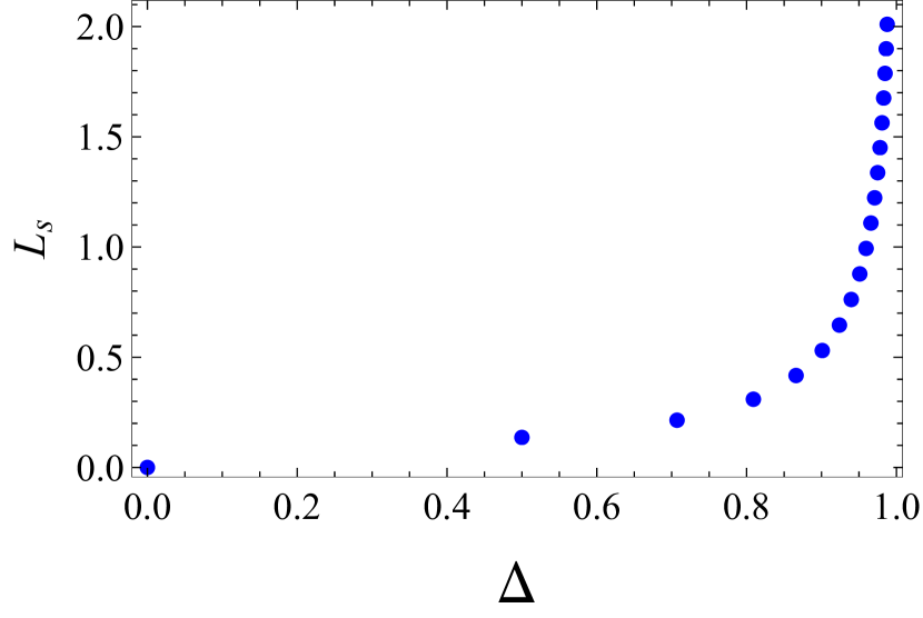
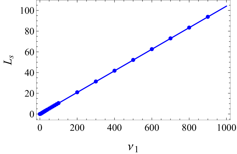
Figure 1: $L_{\textrm{s}}$ for $\frac{\theta}{\pi}=\frac{1}{\nu_{1}}$ at $\beta,h\rightarrow 0$. On the left graph the values are parametrized via $\Delta$ for $\nu_{1}\in[2,20]$. On the right they are parametrized for $\nu_{1}\in[2,30]$ and for $\nu_{1}=35,40,50,60,70,80,90,100,200,300,400,500,600,700,800,900$.

In the case of 2-step fraction we plotted the values of $L_{\textrm{s}}$ for $\nu_{1}=2$ and $\nu_{2}\geq 2$ in Figure 4, where $\Delta$ is confined to $0<\Delta\leq\cos\pi/(2+1/2)\approx 0.31$. In this range the $L_{\textrm{s}}$ increases for large $\nu_{2}$ and diverges at the $\nu_{2}\rightarrow\infty$ limit. For 3-step fraction we plotted the values for $\nu_{1}=\nu_{2}=2,\;\nu_{3}\geq 2$ in Figure 4, where $\Delta$ is confined narrower: the lower bound is $\Delta\approx 0.26$ and the upper bound is the same as in the former case. We also show Figure 4 for 4-step fraction. These results coincide with the suggestion that the spin diffusion diverges everywhere for the anisotropy [10].

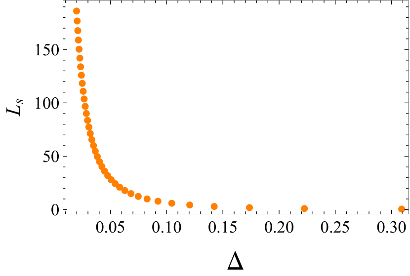
Figure 2: $L_{\textrm{s}}$ for $\frac{\theta}{\pi}=\frac{1|}{|2}+\frac{1|}{|\nu_{2}}$;  $\nu_{2}\in[2,39]$ at $\beta,h\rightarrow 0$

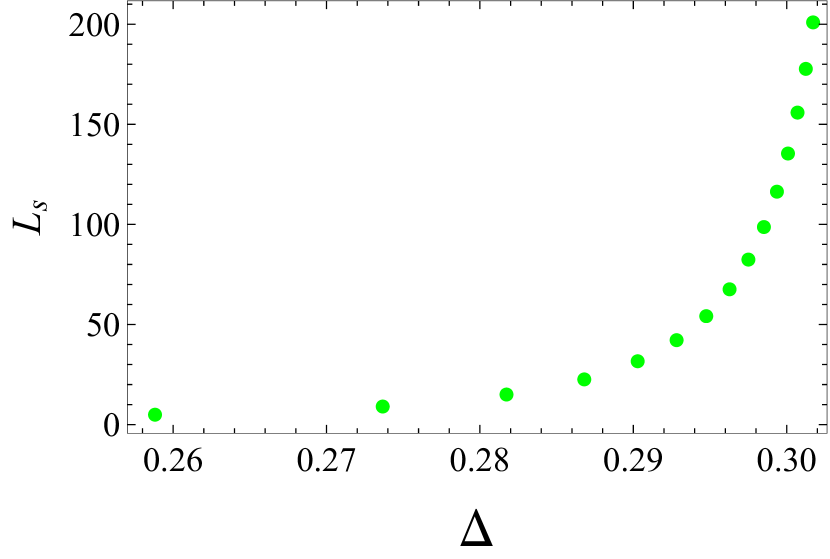
Figure 3: $L_{\textrm{s}}$ for $\frac{\theta}{\pi}=\frac{1|}{|2}+\frac{1|}{|2}+\frac{1|}{|\nu_{3}}$;  $\nu_{3}\in[2,16]$ at $\beta,h\rightarrow 0$

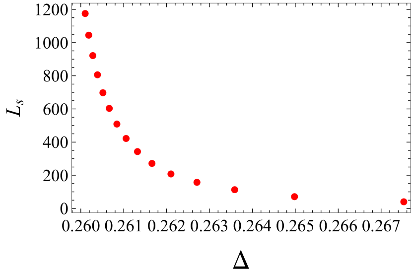
Figure 4: $L_{\textrm{s}}$ for $\frac{\theta}{\pi}=\frac{1|}{|2}+\frac{1|}{|2}+\frac{1|}{|2}+\frac{1|}{|\nu_{4}}$;  $\nu_{4}\in[2,16]$ at $\beta,h\rightarrow 0$

6 Conclusion

The spin element $L_{\textrm{s}}$ of Onsager matrix for spin-$\frac{1}{2}$ critical XXZ chain has been computed at the $\beta,\;h\rightarrow 0$ limit. The dressed scattering kernels $T^{\textrm{dr}}_{j,k=m_{\alpha}-1}$ are involved in the formula of $L_{\textrm{s}}$ at zero magnetic field. They satisfy coupled integral equations, which coincide with the difference between spin $S=(\tilde{n}_{m_{\alpha}}-1)/2$ and $y_{\alpha-1}/2$ TBA equations after derivative with respect to $A\beta$. From this agreement the $T^{\textrm{dr}}_{j,m_{\alpha}-1}$ have been derived from our solutions for higher spin TBA equations, yielding the explicit formula of the $L_{\textrm{s}}$ written by known functions at the $\beta,\;h\rightarrow 0$ limit.

Combining the results in previous section we obtain Figure 5. At the $\beta,h\rightarrow 0$ limit the $L_{\textrm{s}}$ diverges at every length of the continued fractions, if the last step number $\nu_{\alpha}$ goes to infinity. The longer the fraction is, the faster it diverges. This structure will continue deeper and deeper infinitely in a fractal way. From these observations we may expect that the $L_{s}$ is discontinuous with an infinite gap almost everywhere the anisotropy is parametrized by the fractions.

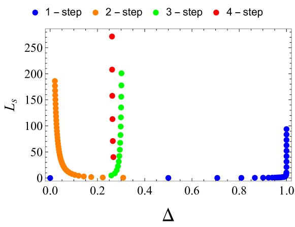
Figure 5: $L_{\textrm{s}}$ for the same continued fractions as in Figure 1, 4, 4 and 4 at $\beta,h\rightarrow 0$

Appendix A Takahashi-Suzuki (TS) numbers

We define a series of real numbers $\{p_{r}\}^{\alpha}_{r=0}$ and series of integers $\{\nu_{i}\}^{\alpha}_{r=1},\{m_{r}\}^{\alpha}_{r=0}$ and $\{y_{r}\}^{\alpha}_{r=-1}$ as follows:

$$p_{0}=\frac{\pi}{\theta},\quad p_{1}=1,\quad\nu_{r}=\left[\frac{p_{r-1}}{p_{r}}\right],\quad p_{r}=p_{r-2}-\nu_{r-1}p_{r-1}\quad(2\leq r\leq\alpha),$$

$$m_{0}=0,\quad m_{r}=\nu_{1}+\nu_{2}+\cdots+\nu_{r}\quad(1\leq r\leq\alpha),$$

$$y_{-1}=0,\quad y_{0}=1,\quad y_{1}=\nu_{1}\;\;\mathrm{and}\;\;y_{r}=y_{r-2}+\nu_{r}y_{r-1}\quad(1\leq r\leq\alpha).$$ (A.1)

Here [x] denotes the maximum integer less than or equal to $x$ (Gauss’ symbol). It is clear that $\frac{1}{p_{0}}$ is given by the continued fraction (2.3). The general rule to determine the length $n$ and parity $v$ of string was given by [12] as follows:

$$n_{j}=y_{r-1}+(j-m_{r})y_{r}\quad(m_{r}\leq j<m_{r+1}),$$

$$n_{m_{\alpha}}=y_{\alpha-1},$$

$$v_{m_{1}}=-1\;\;\mathrm{and}\;\;v_{j}=e^{i\pi[(n_{j}-1)/p_{0}]}\quad(j\neq m_{1}).$$ (A.2)

The series $\{n_{j}\}_{j\geq 1}$ is the TS numbers. We also need the modified TS numbers $\{\tilde{n}\}_{j\geq 1}$ which were introduced by [17] as follows:

$$\tilde{n}_{j}=y_{r-1}+(j-m_{r})y_{r}\quad(m_{r}<j\leq m_{r+1}).$$ (A.3)

Appendix B Relations between the scattering kernels $T_{j,k}$

$T_{j,k}$ satisfy the following relations, which were given by (9.65) in [13]:

$$T_{0,k}= \;0,$$

$$T_{j,k}= \;(1-2\delta_{m_{r-1},j})s_{r}*T_{j-1,k}+s_{r}*T_{j+1,k}+(-1)^{r+1}(\delta_{j-1,k}+\delta_{j+1,k})s_{r}$$

$$\textrm{for}\quad m_{r-1}\leq j\leq m_{r}-2,\quad j\neq m_{\alpha}-2,$$

$$T_{m_{r}-1,k}= \;(1-2\delta_{m_{r-1},m_{r}-1})s_{r}*T_{m_{r}-2,k}+d_{r}*T_{m_{r}-1,k}$$

$$+s_{r+1}*T_{m_{r},k}+(-1)^{r+1}(\delta_{m_{r}-2,k}s_{r}+\delta_{m_{r}-1,k}d_{r}-\delta_{m_{r},k}s_{r+1})$$

$$\textrm{for}\quad r<\alpha,$$

$$T_{m_{\alpha}-2,k}= \;(1-2\delta_{m_{\alpha-1},m_{\alpha}-2})s_{\alpha}*T_{m_{\alpha}-3,k}+s_{\alpha}*T_{m_{\alpha}-1,k}$$

$$+(-1)^{\alpha+1}(\delta_{m_{\alpha}-3,k}+\delta_{m_{\alpha}-1,k}-\delta_{m_{\alpha},k})s_{\alpha},$$

$$T_{m_{\alpha}-1,k}= -T_{m_{\alpha},k}=s_{\alpha}*T^{\textrm{dr}}_{m_{\alpha}-2,k}+\sigma_{k}\delta_{m_{\alpha}-2,k}s_{\alpha}.$$ (B.1)

Appendix C TBA equations for the critical XXZ chain with arbitrary spin $S=\frac{\sigma}{2}\;(\sigma\in\mathbb{N})$

The TBA equations are non-linear integral equations with the following unknown functions:

$$\eta_{j}:=\frac{\rho^{\mathrm{h}}_{j}}{{\rho_{j}}}\quad(1\leq j\leq m_{\alpha}-1),\qquad\eta_{m_{\alpha}}:=\frac{{\rho_{m_{\alpha}}}}{\rho^{\mathrm{h}}_{m_{\alpha}}}.$$ (C.1)

For the chains with arbitrary spin $S=\frac{\sigma}{2}\;(\sigma\in\mathbb{N})$, these functions are determined by the following equations [11]:

$$\eta_{0}= \;0,$$

$$\ln\eta_{j}= \;(1-2\delta_{m_{r-1},j})s_{r}*\ln(1+\eta_{j-1})+s_{r}*\ln(1+\eta_{j+1})$$

$$+(-1)^{r+1}\delta_{j_{\sigma}-1,j}A\beta s_{r}$$

$$\textrm{for}\quad m_{r-1}\leq j\leq m_{r}-2,\quad j\neq m_{\alpha}-2,$$

$$\ln\eta_{m_{r}-1}= \;(1-2\delta_{m_{r-1},m_{r}-1})s_{r}*\ln(1+\eta_{m_{r}-2})+d_{r}*\ln(1+\eta_{m_{r}-1})$$

$$+s_{r+1}*\ln(1+\eta_{m_{r}})+(-1)^{r+1}\Theta(r_{\sigma}+\delta_{j_{\sigma},m_{r}}-r)A\beta d_{r}^{(\sigma)}$$

$$\textrm{for}\quad r<\alpha,$$

$$\ln\eta_{m_{\alpha}-2}= \;(1-2\delta_{m_{\alpha-1},m_{\alpha}-2})s_{\alpha}*\ln(1+\eta_{m_{\alpha}-3})+s_{\alpha}*\ln(1+\eta_{m_{\alpha}-1})(1+\eta^{-1}_{m_{\alpha}})$$

$$+(-1)^{\alpha+1}\delta_{j_{\sigma}-1,m_{\alpha}-2}A\beta s_{\alpha},$$

$$\ln\eta_{m_{\alpha}-1}-y_{\alpha}\beta h= \;y_{\alpha}\beta h-\ln\eta_{m_{\alpha}}=s_{\alpha}*\ln(1+\eta_{m_{\alpha}-2})+(-1)^{\alpha+1}\delta_{j_{\sigma},m_{\alpha}}A\beta s_{\alpha}\;.$$ (C.2)

At high temperature and zero magnetic field the $\eta_{j}$ can be expanded up to $O(\beta)$ in the same way as done in [11]:

$$\eta_{j}(x) =\left(\frac{\tilde{n}_{j+1}}{y_{r}}\right)^{2}\left[1+\frac{A\beta}{2}\left\{f_{j}^{(\sigma)}(x)+g_{j}^{(\sigma)}(x)\right\}\right]-1+O(\beta^{2})$$

$$\textrm{for}\quad m_{r}\leq j<m_{r+1},\quad j\leq m_{\alpha}-2,$$

$$\eta_{m_{\alpha}-1}(x) =\eta_{m_{\alpha}}^{-1}(x)=\frac{y_{\alpha}}{y_{\alpha-1}}\left\{1-\frac{A\beta}{y_{\alpha-1}}f_{m_{\alpha}-1}^{(\sigma)}(x)\right\}-1+O(\beta^{2}),$$ (C.3)

where

$$f_{j}^{(\sigma)}(x)=\sum_{s=1}^{\sigma}\frac{s(s-1)}{\sigma+1}\left[\frac{\tilde{n}_{j+2}}{y_{r}\tilde{n}_{j+1}}\left\{b_{q_{j}}(x+i(\tilde{q}_{j_{\sigma}}+2s))+b_{q_{j}}(x-i(\tilde{q}_{j_{\sigma}}+2s))\right\}\right.$$

$$\qquad\qquad\qquad\qquad\qquad\left.-\frac{n_{j}}{y_{r}\tilde{n}_{j+1}}\left\{b_{\tilde{q}_{j+2}}(x+i(\tilde{q}_{j_{\sigma}}+2s))+b_{\tilde{q}_{j+2}}(x-i(\tilde{q}_{j_{\sigma}}+2s))\right\}\right],$$

$$f^{(\sigma)}_{m_{\alpha}-1}(x)=\sum_{j=1}^{\sigma}\frac{j(\sigma+1-j)}{\sigma+1}b_{q_{m_{\alpha}-1}}(x+i(\tilde{q}_{j_{\sigma}}+2j)),$$

$$g_{j}^{(\sigma)}(x)=\sigma\left[\frac{1}{y_{r}}\sum_{s=1}^{y_{r}}\left\{b_{\tilde{q}_{j_{\sigma}}}(x+i(q_{j}-2s))+b_{\tilde{q}_{j_{\sigma}}}(x-i(q_{j}-2s))\right\}\right.$$

$$\qquad\qquad\qquad-\frac{1}{\tilde{n}_{j+1}}\sum_{s=1}^{\tilde{n}_{j+1}}\left\{b_{\tilde{q}_{j_{\sigma}}}(x+i(q_{j}+2s))+b_{\tilde{q}_{j_{\sigma}}}(x-i(q_{j}+2s))\right\}$$

$$\qquad\qquad\qquad\left.-\frac{n_{j}}{y_{r}\tilde{n}_{j+1}}b_{\tilde{q}_{j+2}+\tilde{q}_{j_{\sigma}}}(x)+\frac{1}{y_{r}}b_{q_{j}+\tilde{q}_{j_{\sigma}}}(x)+\frac{1}{\tilde{n}_{j+1}}b_{q_{j}-\tilde{q}_{j_{\sigma}}}(x)\right],$$

$$b_{q}(x)=\frac{\theta}{2\pi}\frac{\sin\theta q}{\cosh\theta x-\cos\theta q}.$$ (C.4)

Appendix D TBA equations and thermodynamic quantities for spin-$\frac{1}{2}$ critical XXZ chain

The TBA equations for the chain were given by [12] as follows:

$$\mathrm{ln}\;\eta_{j}=\beta\epsilon_{j}+\sum_{k=1}^{m_{\alpha}}T_{j,k}*\mathrm{sign}(q_{k})\mathrm{ln}(1+\eta^{-1}_{k})\;,\quad j=1,2,\cdots,m_{\alpha},$$

$$\epsilon_{j}=Aa_{j}+2n_{j}h.$$ (D.1)

The functions $a_{j}(x)$ are written as

$$a_{j}(x)=-(2\pi)^{-1}\frac{d}{dx}k_{j}(x)=\frac{\theta}{2\pi}\frac{\sin\theta q_{j}}{\cosh\theta x+\cos\theta q_{j}},$$ (D.2)

$$k_{j}(x)=\frac{1}{i}\mathrm{ln}\left\{\frac{\sinh\frac{\theta}{2}(x+in_{j}+ip_{0}(1-v_{j})/2)}{\sinh\frac{\theta}{2}(x-in_{j}+ip_{0}(1-v_{j})/2)}\right\},$$ (D.3)

$$q_{j}=(-1)^{r}(p_{r}-(j-m_{r})p_{r+1})\quad(m_{r}\leq j<m_{r+1}),$$ (D.4)

Here $v_{j}$ is the parity of string given by (A.2). Using (B.1) one can rewrite (D.1) as follows:

$$\eta_{0}= \;0,$$

$$\ln\eta_{j}= \;(1-2\delta_{m_{r-1},j})s_{r}*\ln(1+\eta_{j-1})+s_{r}*\ln(1+\eta_{j+1})+\delta_{j,1}A\beta s_{1}$$

$$\textrm{for}\quad m_{r-1}\leq j\leq m_{r}-2,\quad j\neq m_{\alpha}-2,$$

$$\ln\eta_{m_{r}-1}= \;(1-2\delta_{m_{r-1},m_{r}-1})s_{r}*\ln(1+\eta_{m_{r}-2})+d_{r}*\ln(1+\eta_{m_{r}-1})$$

$$+s_{r+1}*\ln(1+\eta_{m_{r}})$$

$$\textrm{for}\quad r<\alpha,$$

$$\ln\eta_{m_{\alpha}-2}= \;(1-2\delta_{m_{\alpha-1},m_{\alpha}-2})s_{\alpha}*\ln(1+\eta_{m_{\alpha}-3})+s_{\alpha}*\ln(1+\eta_{m_{\alpha}-1})(1+\eta^{-1}_{m_{\alpha}}),$$

$$\ln\eta_{m_{\alpha}-1}-y_{\alpha}\beta h= \;y_{\alpha}\beta h-\ln\eta_{m_{\alpha}}=s_{\alpha}*\ln(1+\eta_{m_{\alpha}-2}).$$ (D.5)

If we put $\sigma=1$ in (C.2) the result coincides with (D.5). Thus the solutions for (D.5) are obtained from (C.3) at high temperature and zero magnetic field as follows:

$$\eta_{j}(x) =\left(\frac{\tilde{n}_{j+1}}{y_{r}}\right)^{2}\left[1+\frac{A\beta}{2}\left\{\frac{\tilde{n}_{j+2}}{y_{r}\tilde{n}_{j+1}}a_{j}(x)-\frac{n_{j}}{y_{r}\tilde{n}_{j+1}}\tilde{a}_{j+2}(x)\right\}\right]-1+O(\beta^{2})$$

$$\textrm{for}\quad m_{r}\leq j<m_{r+1},\quad j\leq m_{\alpha}-2,$$

$$\eta_{m_{\alpha}-1}(x) =\eta_{m_{\alpha}}^{-1}(x)=\frac{y_{\alpha}}{y_{\alpha-1}}\left\{1+\frac{A\beta}{2y_{\alpha-1}}a_{m_{\alpha}-1}(x)\right\}-1+O(\beta^{2}),$$ (D.6)

where

$$\tilde{a}_{j}(x)=\frac{\theta}{2\pi}\frac{\sin\theta\tilde{q}_{j}}{\cosh\theta x+\cos\theta\tilde{q}_{j}},$$ (D.7)

$$\tilde{q}_{j}=(-1)^{r}(p_{r}-(j-m_{r})p_{r+1})\quad(m_{r}<j\leq m_{r+1}).$$ (D.8)

Differentiating (D.1) with respect to Lagrange parameters $\beta_{i}$ yields

$$\epsilon_{i;j}=\varepsilon_{i;j}+\sum_{k=1}^{m_{\alpha}}T_{j,k}*\mathrm{sign}(q_{k})\vartheta_{k}\varepsilon_{i;k},$$ (D.9)

$$\epsilon_{i;j}:=\frac{\partial\beta\epsilon_{j}}{\partial\beta_{i}},\quad\varepsilon_{i;j}:=\frac{\partial\;\mathrm{ln}\;\eta_{j}}{\partial\beta_{i}}.$$ (D.10)

Here $\varepsilon_{i;j}$ are the dressed functions of $\epsilon_{i;j}$ in which $\varepsilon_{1,j}$ are the dressed energies and $\varepsilon_{0;j}=:s^{\textrm{dr}}_{j}$ are the dressed spins. Differentiating (D.5) with respect to $\beta_{i}=2h/T$ at the $h\rightarrow 0$ limit, we have

$$s^{\textrm{dr}}_{j}=0\quad(1\leq j\leq m_{\alpha}-2),\qquad s^{\textrm{dr}}_{m_{\alpha}-1}=s^{\textrm{dr}}_{m_{\alpha}}=\frac{y_{\alpha}}{2}.$$ (D.11)

We also differentiate (D.1) with respect to $A\beta$, which yields

$$\frac{\partial\mathrm{ln}\;\eta_{j}}{\partial A\beta}=a_{j}-\sum_{k=1}^{m_{\alpha}}T_{j,k}*\mathrm{sign}(q_{k})\vartheta_{k}\frac{\partial\mathrm{ln}\;\eta_{j}}{\partial A\beta}.$$ (D.12)

Comparing this with (3.3), we have

$$\rho_{j}(x)+\rho_{j}^{\mathrm{h}}(x)=\mathrm{sign}(q_{j})\frac{\partial\ln\eta_{j}(x)}{\partial A\beta}.$$ (D.13)

Using this and (C.1), we also have

$$\frac{\rho_{j}(x)\rho_{j}^{\mathrm{h}}(x)}{\rho_{j}(x)+\rho_{j}^{\mathrm{h}}(x)}=\frac{\eta_{j}(x)}{(1+\eta_{j}(x))^{2}}\mathrm{sign}(q_{j})\frac{\partial\ln\eta_{j}(x)}{\partial A\beta}.$$ (D.14)

We write the dressed momenta as $k^{\textrm{dr}}_{j}.$ Comparing (D.12) with (D.7), we have

$$\partial_{x}k^{\textrm{dr}}_{j}=-2\pi\partial_{A\beta}\mathrm{ln}\;\eta_{j}.$$ (D.15)

Thus the effective velocities $v^{\mathrm{eff}}_{j}$ are written as

$$v^{\mathrm{eff}}_{j}(x):=\frac{\partial_{x}\varepsilon^{\textrm{dr}}_{j}}{\partial_{x}k^{\textrm{dr}}_{j}}=-\frac{\beta^{-1}\partial_{x}\ln\eta_{j}(x)}{2\pi\partial_{A\beta}\ln\eta_{j}(x)}.$$ (D.16)

Using the following equation from (D.5):

$$\ln\eta_{m_{\alpha}-1}-y_{\alpha}\beta h=y_{\alpha}\beta h-\ln\eta_{m_{\alpha}}\;,$$ (D.17)

we have

$$v^{\mathrm{eff}}_{m_{\alpha}-1}=v^{\mathrm{eff}}_{m_{\alpha}}.$$ (D.18)

At the $h\rightarrow 0$ limit we also have the followings, using (C.1), (D.15), (D.17) and $q_{m_{\alpha}-1}=-q_{m_{\alpha}}$:

$$\rho_{m_{\alpha}-1}=\rho_{m_{\alpha}},\quad\rho^{\mathrm{h}}_{m_{\alpha}-1}=\rho^{\mathrm{h}}_{m_{\alpha}}.$$ (D.19)

References

[1]
O. A. Castro-Alvaredo, B. Doyon and Takato Yoshimura,
“Emergent Hydrodynamics in Integrable Quantum Systems out of Equilibrium”,
Physical Review X 6, 041065 (2016).
[2]
B. Bertini, M. Collura, J. D. Nardis and M. Fagotti
“Transport in Out-of-Equilibrium XXZ Chains: Exact Profiles of Charges and Currents”,
Physical Review Letters 117, 207201 (2016).
[3]
B. Doyon,
“Lecture notes on Generalised Hydrodynamics”,
SciPost Phys. Lect. Notes 18 (2020) · published 28 August 2020.
[4]
M. Rigol and M. Srednichi,
“Alternatives to Eigenstate Thermalization”,
Physical Review Letters 108, 110601 (2012).
[5]
M. Rigol, A. Muramatsu and M. Olshanii,
“Hard-core bosons on optical superlattices: Dynamics and relaxation in the superfluid and insulating regimes”,
Physical Review A 74, 053616 (2006).
[6]
M. Rigol, V. Dunjko, V. Yurovsky and M. Olshanji,
“Relaxation in a Completely Integrable Many-Body Quantum System: An Ab Initio Study of the Dynamics of the Highly Excited States of 1D Lattice Hard-Core Bosons”,
Physical Review Letters 98, 050405 (2007).
[7]
L. Vidmar and M. Rigol,
“Generalized Gibbs ensemble in integrable lattice models”,
Journal of Statistical Mechanics: Theory and Experiment, 064007 (2016)
[8]
B. Doyon and H. Spohn
“Drude weight for the Lieb-Liniger Bose gas”,
SciPost Phys. 3, 039 (2017).
[9]
J. D. Nardis, D. Bernard and B. Doyon,
“Diffusion in generalized hydrodynamics and quasi-particle scattering”,
SciPost Phys. 6, 049 (2019).
[10]
E. Ilievski, J. D. Nardis, M. Medenjak and T. Prosen,
“Superdiffusion in One-Dimensional Quantum Lattice Models”,
Physical Review Letters 121, 230602 (2018).
[11]
S. Ae and K. Sakai
“Spin Drude weight for the integrable XXZ chain with arbitrary spin”,
arXiv:2309.16462v1 [cond-mat.stat-mech] 28 Sep 2023.
[12]
M. Takahashi and M. Suzuki,
“One-Dimensional Anisotropic Heisenberg Model at Finite Temperatures”,
Prog. Theor. Phys. 48, 2187 (1972).
[13]
M. Takahashi,
“Thermodynamics of One-dimensional Solvable Models”,
Cambridge University Press (1999).
[14]
E. Ilievski,
“Popcorn drude weights from quantum symmetry”,
Journal of Physics A: Mathematical and Theoretical, 55(50):504005, 2023.
[15]
C.N. Yang and C.P. Yang, J. Math. Phys. 10 (1969), 1115.
[16]
S. Gopalakrishnan and R. Vasseur,
“Kinetic theory of spin diffusion and superdiffusion in XXZ spin chains”,
Phys. Rev. Letters 122, 127202 (2019).
[17]
A. Kuniba, K. Sakai, J. Suzuki,
“Continued fraction TBA and functional relations in XXZ model at root of unity”,
Nucl. Phys. B 525, 597 (1998).