Cyber Insurance Risk: Reporting Delays, Third-Party Cyber Events, and Changes in Reporting Propensity - An Analysis Using Data Breaches Published by U.S. State Attorneys General

Abstract

With the rise of cyber threats, cyber insurance is becoming an important consideration for businesses. However, research on cyber insurance risk has so far been hindered by the general lack of data, as well as limitations underlying what limited data are available publicly. Specifically and of particular importance to cyber insurance modelling, limitations arising from lack of information regarding (i) delays in reporting, (ii) all businesses affected by third-party events, and (iii) changes in reporting propensity. In this paper, we fill this important gap by utilising an underrecognised set of public data provided by U.S. state Attorneys General, and provide new insights on the true scale of cyber insurance risk. These data are collected based on mandatory reporting requirements of data breaches, and contain substantial and detailed information. We further discuss extensively the associated implications of our findings for cyber insurance pricing, reserving, underwriting, and experience monitoring.

1 Introduction

As the Internet and other digital networks are becoming increasingly vital to the functioning of the global economy, the threat posed by cybercriminals has risen in prominence (OECD, 2020). Cybercrime will result in an estimated economic loss of $\$$8 trillion USD in 2023, with the figure expected to rise to $\$$10.5 trillion annually by 2025 (Cybersecurity Ventures, 2022). Cyber is identified as the greatest risk faced by organisations globally, consecutively for 2021 and 2022 (Allianz, 2022, 2023), and the most significant threat to both U.S. financial institutions and the overall financial system (Aon, 2021).

In addition to adopting effective cyber hygiene practices, businesses are turning to cyber insurance policies for financial coverage and expert guidance in preventing and managing cyber incidents (Deloitte, 2020). Cyber insurance direct written premiums in the U.S. in 2021 were around $\$$6.5 billion USD, an increase of 61$\%$ from 2020 (National Association of Insurance Commissioners, 2022). The global estimated gross direct premiums written in 2022 reached approximately $\$$14 billion USD, with the U.S. contributing more than half of the total (Insurance Business, 2023). A survey conducted by Marsh and Microsoft found that 61$\%$ of organisations purchase some type of cyber insurance (Marsh, 2022).

To more accurately price cyber insurance, researchers study the statistical properties of various types of cyber incidents and propose different approaches to modelling their frequency and/or severity. However, one of the key challenges is the shortage of publicly accessible, credible, comprehensive, and extensive datasets (Zeller and Scherer, 2021). Most literature uses the data breach database provided by Privacy Rights Clearinghouse (2023a), as it is regarded as the only usable public dataset for data breaches so far (notably Wheatley et al., 2016; Edwards et al., 2016; Eling and Loperfido, 2017; Eling and Jung, 2018; Xu et al., 2018; Sun et al., 2021; Bessy-Roland et al., 2021; Wheatley et al., 2021; Lu et al., 2021; Farkas et al., 2021; Li and Mamon, 2023; Liu et al., 2022; Poyraz et al., 2020). For the rest of this paper, we will refer to this dataset as the PRC dataset . Li and Mamon (2023) study medical data breaches compiled by the PRC dataset and the U.S. Department of Health and Human Services; the latter is also publicly available (U.S. Department of Health and Human Services, 2023). Some literature models cyber events beyond data breaches using commercial datasets or claims data provided by a single insurer (notably Jung, 2021; Eling and Wirfs, 2019; Romanosky, 2016; Kesan and Zhang, 2020; Strupczewski, 2019; Malavasi et al., 2022; Palsson et al., 2020; Shevchenko et al., 2021; Eling et al., 2022).

However, due to the lack of available data points and data issues inherent in the PRC dataset, the value of both frequency modelling and the identification of frequency trends to cyber insurers in the literature is diminished. 1) Incurred But Not Reported (IBNR) breaches are not developed because delays in reporting are ignored due to the lack of information on the date of breach occurrence in the PRC dataset. 2) In the event of a third-party data breach, the PRC dataset excludes some businesses for which cyber insurers potentially bear liability. 3) Due to changes in the reporting propensity of the PRC dataset over time, the identified frequency trends based on this dataset may not reflect the actual trends in occurred events. In the next paragraphs, we explain why these considerations are important for cyber insurers.

First, it should be noted that the PRC dataset only includes the date of breach notification, lacking information about the date of breach occurrence. As a result, limited research exists that studies the notification lags of cyber events to inform reserving; this is discussed in more detail in Section 4. As required by the National Association of Insurance Commissioners (NAIC), property and casualty insurers in the U.S. need to file quarterly financial statements (National Association of Insurance Commissioners, 2023b). As cyber insurers quantify their liabilities quarterly, changes in quarterly development profiles should be monitored to build an accurate estimation of incurred but not reported (IBNR) breaches. The development profile/pattern or reporting pattern refers to the pattern or trend over time of event notifications to insurers following the occurrence of a cyber event. With the lack of projection of IBNR breaches due to the issue identified above, the frequency modelling and any frequency trends revealed in the literature can be improved.

Second, the number of events recorded in the PRC dataset may have underrated the true risk landscape faced by cyber insurers and the actual impact of data breaches. This underestimation occurs because the PRC dataset considers each third-party data breach as a single event occurred at one of the affected organisations, instead of multiple events occurred at each of all affected organisations. A third-party data breach refers to a data breach that occurs at a service provider, vendor, or other third-party organisation that has access to other companies’ data (Prevalent, 2022). Such a breach not only affects the third-party provider, but its client firms whose data are compromised or exposed as a result of its failure. In the event of a third-party data breach, cyber insurers are responsible for affected organisations which purchase insurance with them, whether they be the third-party provider or its affected client firms. Therefore, from the insurer’s perspective, when counting the number of events, we should consider each affected organisation as a separate event, in case of a third-party data breach.

Third, the publicly disclosed events in the PRC dataset may not be suitable for monitoring changes in occurred events over time due to the lack of reasonable assumptions regarding the reporting propensity of the dataset. The reporting propensity refers to the ratio of the number of breaches reported in a period to those actually occurring. The reporting propensity of the PRC dataset, which collects national data breaches, is likely to vary over time due to material differences in data breach notification requirements across states and over time. Consequently, counts of reported events do not validly reflect any trend in those incurred.

This paper aims to fill the aforementioned gaps, by utilising an underrecognised set of public data consisting of individual state Attorneys General’s publications of data breaches in the United States. These data 1) are collected in accordance with mandatory state data breach notification laws, 2) provide informative descriptions of data breaches, and 3) constitute one of the primary sources of existing datasets, including the PRC dataset and some commecial datasets such as Advisen. Our analysis of the frequency information in this set of data can help cyber insurers more accurately estimate IBNR reserves and gain a more comprehensive understanding of data breach claim frequency over time.

First, as state Attorneys’ General provide date of breach occurrence, we examine the time lag between data breach occurrence and reporting to state regulators, which approximates the notification lag of data breach claims for insurers, by state and severity of the breach. We also study data breach frequency trends, which approximate claim frequency trends, after projecting IBNR breaches using standard insurance practices in claims reserving (Mack, 1994, 1993; Renshaw and Verrall, 1998; England and Verrall, 2002; Taylor, 2012; Wüthrich and Merz, 2008; Peremans et al., 2017; Sriram and Shi, 2021; Antonio and Beirlant, 2008; Pinheiro et al., 2003; Shi, 2017).

As our modelling attends to the fine detail of the data, we are able to extract features from the frequency data that have not been mentioned in the prior literature. An understanding of these features, such as the commonalities among states and severities measured by the number of affected state residents, is of considerable value to pricing, reserving, and general appreciation of the evolution of cyber experience. Our analysis may serve as an example of the kind of analysis that could be performed on cyber data elsewhere.

Second, in the case of a third-party data breach, it is mandatory for the third-party vendor and its affected client firms to report to state Attorneys’ General. The reporting obligation for an individual business, whether it be the third-party vendor or an affected client firm, depends on whether the specific incident that it experienced meets the state’s reporting requirement. This enables us to assess the frequency of data breaches for which cyber insurers bear liability.

Third, we take into account differences in data breach notification obligations across states and over time when selecting and analysing frequency data, in order to more reliably identify the development of occurred events over time. For example, we analyse state Attorneys General’s publications individually. As the data breach notification obligations imposed on each state do not undergo significant changes, it is reasonable to assume that each state is subject to a relatively constant reporting propensity over time.

Our analysis provides important insights. The development profiles of data breaches with various severities measured by the number of affected state residents have shifted over time. Breaches which affect more state residents experience longer delays on average than breaches which affect less. The average delay of data breaches, between the first possible date of breach occurrence and the date reported to government bodies, has lengthened to different extents in different states after 2017 compared to prior periods. Different states follow highly similar frequency trends. They are relatively stationary up to the first quarter of 2020 but increasing subsequently. While there are variations in the development profiles of data breaches among states, states not only demonstrate similar breach frequency trends and trends in the average delay mentioned above, but also share the timing of change in reporting patterns. The historical change in the development profile of various states commences at a similar point in time, around 2017.

The main takeaway from this analysis is that overly simple modelling of frequency data that is subject to increasing reporting delay is unlikely to capture the full extent of the increase, and this would lead to underestimation of IBNR, and hence of breach frequency. We also extensively discuss the insurance implications of the above findings on pricing, reserving, underwriting, capital needs, and experience monitoring. Details are provided later in Section 6.

The paper is organised as follows. Section 2 distinguishes state Attorneys General’s datasets from the PRC dataset and discusses data analysis considerations for cyber data. Section 3 outlines the selection and processing of state Attorneys General’s data before they are modelled. Section 4 describes the construction of the model used in this paper. Section 5 provides details of the model output, including the discovery of data features not mentioned in prior literature that could provide valuable insights into cyber risk. Section 6 highlights key research findings of this paper for academic researchers and cyber insurers, including a detailed discussion of the insurance implications of the main model output found in Section 5. Section 7 concludes.

2 State Attorneys General’s publications of data breaches

This section contains two parts. First, we introduce the datasets of state Attorneys General in Section 2.1. As they have not yet been sufficiently acknowledged by the literature, we offer some background for cyber risk researchers to understand the differences among the datasets of individual state Attorneys General. State Attorneys General’s publications should serve as important data sources in the current climate of scarce public data on cyber events, as they constitute one of the primary sources of major existing datasets and provide comprehensive and valuable information.

Second, in Section 2.2, we compare state Attorneys General’s datasets with the most commonly used public dataset of data breaches (the PRC dataset), in order for academic researchers to better utilise these two data sources to gain insights into data breach risks. From the perspective of understanding and modelling the risks of data breaches over time, datasets of state Attorneys General have some advantages over the PRC dataset. State Attorneys General’s data contain more extensive and detailed information of data breaches (see Section 2.2.1). Furthermore, they provide a more detailed description of data breaches that affect multiple businesses due to the use of common services and providers, revealing the resulting interdependence of businesses (see Section 2.2.2). This has significant value in understanding the consequences of dependent cyber policies, which is the major impediment to the market’s expansion. In addition, as we could more confidently assume a constant reporting propensity for this set of data, the frequency trend of reported breaches appears to be a more accurate depiction of the actual breaches that have occurred (see Section 2.2.3).

2.1 Introduction of public datasets underrepresented by current literature

In this paper, we use data breaches published by individual state Attorneys General in the United States to investigate changes in data breach reporting patterns and frequency trends. These data breaches are subject to state reporting guidelines, and they are publicly accessible on the websites of state Attorneys General (see the references below).

As of June 2023, 17 state Attorneys General publicly publish data breaches that they collect. See State of California Department of Justice (2023); Delaware Department Of Justice (2023); Office of Consumer Protection Hawaii (2023); Indiana Attorney General (2023); Iowa Department of Justice (2023); Office of the Maine Attorney General (2023); Maryland Attorney General (2023); Office of Consumer Protection Montana (2023); New Hampshire Department of Justice (2023); New Jersey Cybersecurity $\&$ Communications Intergration Cell (2023); North Dakota Attorney General (2023); Oklahoma Office of Management $\&$ Enterprise Services (2023); Oregon Department of Justice (2023); Attorney General of Texas (2023); Office of the Vermont Attorney General (2023); Washington State Office of the Attorney General (2023); State of Wisconsin (2023).

2.1.1 Inconsistent data breach notification laws across states and over time in the United States

At this time, the protection of private information in the United States is provided by a mixture of sector-specific federal statutes (i.e., covering financial services, healthcare, telecommunication, and education) and state laws, which differ in their scope and jurisdiction (The International Comparative Legal Guides, 2023). The National Conference of State Legislatures (NCSL) publishes state data breach notification laws in the United States (The National Conference of State Legislatures, 2022). As of June 2023, data breach notification laws have been implemented in all 50 states, the District of Columbia, Guam, Puerto Rico, and the Virgin Islands.

States in the United States imposed their own data breach notification laws at different times, each of which protects the privacy of its residents (The National Conference of State Legislatures, 2022). For instance, California has had a data breach notification law in effect since 2002, Mississippi since 2010, and South Dakota and Alabama in 2018, the last two states to enact such legislation.

While most state data breach notification laws have similar elements, there are still variations. Key disparities include definition of what constitutes personally identifiable information, whom entities must notify, the number of affected state residents above which notification to the state Attorney General becomes mandatory, and when the notification must be made once an obligation is triggered. Additionally, the content of breach notice, whether the state publishes breach data publicly, and any exemptions from reporting also vary across states (Privacy Rights Clearinghouse, 2023b). For example, Table 1 shows the varying definitions of reportable data breaches to state Attorneys General in the U.S. in 2021 (The International Association of Privacy Professionals, 2021). The same breach might require notification of multiple state Attorneys General, if it affects residents from multiple states.

Table 1: Definitions of reportable data breaches in the U.S. in 2021

Notification to state Attorney General	Number of states a
No obligations	17
Yes	14
Yes if more than 250 state residents	4
Yes if more than 500 state residents	8
Yes if more than 1000 state residents	7
Others	4

• including 50 states, District of Columbia, Guam, Puerto Rico, and the Virgin Islands

Additionally, state laws are amended on a regular basis. Common trends include expanding the number of data items that constitute personally identifiable information, reducing reporting timeframe, and requiring notification of the state Attorney General. According to Maine Legislature (2019), an additional requirement of the state Attorney General effective from September 19, 2019 is to report breaches no later than 30 days after their discovery. Table 5 presents the dates when some states’ statutes began to require notification of the Attorney General.

2.1.2 Differing fields contained in the datasets of individual state Attorneys General

Table 2 and 3 distinguish the information provided by individual state Attorneys General on data breaches, as of June 2023. Attorneys General of New Hampshire, New Jersey, Vermont, and Wisconsin also publish breach information, but the breaches are presented only by individual notice letters. The second column of Table 2 lists the notification requirement of the state Attorney General. The fourth and fifth columns of Table 3 present the requirements of maximum notification timeframes from the discovery of a breach. The last column of Table 3 references state statutes.

Table 2: Summary of datasets from state Attorneys General - 1

State	Notification to State Attorney General	Breach notice	Organisation Name	Start of breach date	End of breach date	Reported date	Number of persons affected (state)	Number of persons affected (total)
California	Yes if more than 500 California residents	Y	Y	Y	Y	Y
Delaware	Yes if 500 Delaware residents	Y	Y	Y	Y	Y	Y
Hawaii	Yes if 1000 Hawaii residents	Y	Y	Y	Y	Y	Y
Indiana	Yes		Y	Y		Y	Y	Y
Iowa	Yes if 500 Iowa residents	Y	Y			Y
Maine	Yes	Y after 2020	Y	Y	Y	Y	Y	Y after 2018
Maryland	Yes	Y	Y			Y	Y
Massachusetts	Yes		Y			Y	Y
Montana	Yes	Y	Y	Y	Y	Y	Y
North Dakota	Yes if 250 North Dakota residents	Y	Y	Y	Y	Y	Y
Oregon	Yes if 250 Oregon residents		Y	Y	Y	Y
Texas	Yes if 250 Texas residents		Y			Y	Y
Washington	Yes if 500 Washington residents	Y	Y	Y	Y	Y	Y

Table 3: Summary of datasets from state Attorneys General - 2

State	Cause of breach	Information breached	Timeframe of Notification to Individuals (law enforcement exceptions)	Timeframe of Notification to State Attorney General	Breach Notification Statutes
California			as expediently as possible (AEAP) and “without unreasonable delay” a		Cal. Civ. Code 1798.82 et seq.
Delaware			“without unreasonable delay but no later than 60 days after determination of the breach of security” b	“no later than the time when notice is provided to the resident” b	Del. Code Ann. tit. 6 § 12B-101 et seq.
Hawaii	Y		“without unreasonable delay” c	“without unreasonable delay” c	Haw. Rev. Stat. § 487N-1 et seq.
Indiana			“without unreasonable delay” d	“without unreasonable delay” d	Ind. Code § 24-4.9-1-1 et seq.
Iowa			AEAP and “without unreasonable delay” e	“within 5 business days after giving notice of the breach of security to consumers” e	Iowa Code § 715C.1 – 2
Maine		Y	AEAP and “without unreasonable delay, no more than 30 days after awareness of a breach of security and identification of its scope” f	“without unreasonable delay” f	Me. Rev. Stat. tit. 10 § 1346 et seq.
Maryland	Y	Y	“as soon as reasonably practicable, but no later than 45 days after the business discovers or is notified of the breach of the security of a system” g	“prior to notification to individuals” g	Md. Code Com. Law § 14-3504 et seq.
Massachusetts		Y	“as soon as practicable and without unreasonable delay” h	“without unreasonable delay” h	Mass. Gen. Laws 93H § 1 et seq.
Montana			AEAP and “without unreasonable delay” i	“simultaneous with notification to individual” i	Mont. Code § 30-14-1701 et seq.
North Dakota			AEAP and “without unreasonable delay” j	“without unreasonable delay” j	N.D. Cent. Code § 51-30-01 et seq.
Oregon			AEAP and “without unreasonable delay, but no later than 45 days after discovering or receiving notification of the breach of security” k	“without unreasonable delay, but no later than 45 days after …” k	Or. Rev. Stat. §§ 646A.600 - 646A.604
Texas		Y	“without unreasonable delay and in each case no later than the 60th day after the date on which the person determines that the breach occurred” l	“no later than the 60th day after …” l	Tex. Bus. $\&$ Com. Code § 521.053
Washington		Y	AEAP and “without unreasonable delay, and no more than 30 calendar days after the breach was discovered” m	“no more than 30 days after the breach was discovered” m	Wash. Rev. Code § 19.255.010 et seq.

• California Legislative Information (2023);

• The Delaware Code Online (2023);
  

• Hawaii State Legislature (2023);

• Indiana General Assembly (2023);

• Iowa Legislature (2023);
  

• Maine Legislature (2023);

• Maryland General Assembly (2023);
  

• The 193rd General Court of the Commonwealth of Massachusetts (2023);
  

• Montana Code Annotated 2021 (2023);

• North Dakota Legislative Branch (2023);
  

• OregonLaws (2023);

• Texas Constitution and Statutes (2023);
  

• Washington State Legislature (2023)

2.2 Advantages of datasets from state Attorneys General over the PRC database on frequency modelling

The main dataset used in data breach frequency and severity modelling is the PRC dataset. The PRC dataset obtains most of its data from state Attorneys General and the U.S. Department of Health and Human Services; the former are the data sources of this paper and the latter collects breaches of protected health information under a federal regulation (i.e., The Health Insurance Portability and Accountability Act of 1996 (HIPAA)), which is also publicly available (U.S. Department of Health and Human Services, 2023).

Data from state Attorneys General are more suitable for the purpose of this study than the PRC dataset due to the considerations below.

2.2.1 Additional information provided by state Attorneys General

 Dates of occurrence

As major sources of the PRC dataset, data breaches publicised by state Attorneys General contain the information necessary for assessing reporting delay - date of breach incidence - that is absent from the PRC dataset. Shown in Table 2, among all states that publicly publish data breaches, 8 explicitly present information regarding dates of occurrence (i.e., California, Delaware, Indiana, Maine, Montana, North Dakota, Oregon, and Washington). Maine provides two additional dates, including date of discovery and date of consumer notification.

Data breach notification letters

Some state Attorneys General provide access to data breach notification letters that are submitted by organisations as part of regulatory requirements. These letters typically contain comprehensive descriptions of the breaches that have occurred.

Up-to-date breaches

State Attorneys General are updating their own database daily to include the newest reported data breaches, making the examination of breaches occurred in 2020 and 2021 possible. However, the PRC dataset contains few data breaches which are reported after 2018 and none after 2019, and thus makes it difficult to see the most recent changes, including those affected by the COVID-19 pandemic. Wheatley et al. (2021) find that the number of data breaches in 2018-2019 present in the PRC dataset is far less than those in previous years, suspecting incomplete data. Li and Mamon (2023) suggest that the PRC dataset is only reliable until 2017.

2.2.2 Richer description of data breaches

 Two different event definitions could be used

One of the peculiarities of cyber risk is that event definition can be complicated by interdependencies among certain security incidents (Wheatley et al., 2021), namely third-party cyber events. A third-party data breach, as defined in Section 1, can be considered as 1) a single event occurred at the third-party provider or one of its affected client firms, or 2) a series of correlated events at the provider and all of its affected client firms. The choice of event definition will impact on the derived frequency trend, as the latter will result in a greater number of occurred data breaches.

In the case of a third-party breach, the PRC dataset follows the former event definition (Benaroch, 2021) and datasets of state Attorneys General follows the latter. For example, In 2017, Sabre, a travel company, experienced a data breach in its Hospitality Solutions system that affected its business partners who used its central reservations booking engine (Fortra, 2021). In the PRC dataset, this data breach is recorded as a single event under Sabre. However, state Attorneys General’s datasets classify it as multiple breaches involving various organisations, including Sabre. This is because the affected companies that outsourced services to Sabre were obligated to report the breach to relevant state Attorneys General individually.

Which event definition should be used

According to Wheatley et al. (2021), taking into account all affected organisations in the case of a third-party cyber event provides a richer description of the event. Also, both from an economic and a cyber insurer’s point of view, a third-party data breach should be regarded as a series of events rather than a single occurrence, which will be explained below.

To avoid underestimating the risk of a data breach, a third-party data breach should be viewed as a series of events occurred at both the third-party provider and all of its affected client firms. It should not be considered as a single event occurred at the third-party provider or one of its affected client firms. If not, we would underestimate the total number of businesses that are affected by such a breach, resulting in an overall underestimation of the frequency rate. Second, we would underestimate the economic impact of the third-party data breach, by failing to account for the impact on each of all affected businesses. Third, we would underestimate the dependencies across organisations because the data do not capture the dependence resulting from the utilisation of common services and providers.

From the point of view of cyber insurance pricing, considering all affected businesses in the case of a third-party data breach has significant value in understanding the consequences of dependent cyber policies, which is the major impediment to the market’s expansion. A cyber liability policy covers financial loss in the event of a data breach, irrespective of who was accountable for the loss of data (Woodruff Sawyer, 2020). Therefore, when the insurance company insures a third-party provider and its client firms, a breach occurred at the provider may result in multiple claims to the insurer, rather than a single claim, which can be an aggregation problem.

When the data of an organisation that has purchased cyber insurance is compromised within a third party’s system, the insurer will incur two kinds of costs. First, the organisation is responsible for the costs related to the data breach, including regulatory compliance, potential litigation, and related costs. When the contract with the third-party vendor is not enough to cover these costs, the insurer is responsible for the rest (Woodruff Sawyer, 2020). Second, the insurer may take the lead in executing the organisation’s contractual rights with the service provider directly accountable for the breach. This is known as subrogation (Woodruff Sawyer, 2020).

Third-party data breaches require particular attention, as the “cloud” has become a ubiquitous part of corporate IT networks, and most breaches are found to be caused by third-party vendors. In 2022, 94$\%$ of businesses use cloud services in some capacity to hold and process their data (Flexera, 2022). Ponemon Institute (2022) found that among 1162 cybersecurity experts surveyed, a majority of the them, accounting for 59 percent, acknowledged that their organisations had encountered a data breach originating from third parties.

In addition, the current literature has not investigated trends in data breach frequency that attempt to take into account all affected client firms of the third party vendor in the case of a third-party data breach. Therefore, we use datasets of state Attorneys General in our frequency analysis.

2.2.3 A more constant reporting propensity

  Some assumption about the reporting propensity is required to assess risks over time

The ultimate goal of modelling the frequency and severity of cyber risks in the context of cyber insurance is to estimate the loss distribution of insurance claims resulting from occurred cyber incidents. Trend analysis of occurred events can shed light on the risks associated with insurance claims over time. However, the limitation of any datasets that collect real events is that they can only record those that are publicly disclosed; not all events that have occurred are known.

Nonetheless, we can learn about the trend of actual events by analysing reported ones, so long as we can make a valid assumption about the reporting propensity (see the definition in Section 1). For example, if the reporting propensity remains constant over occurrence periods, then counts of reported events will vary proportionately with those incurred, and the former will validly reflect any trend in the latter.

The data breach reporting propensity in the United States may have shifted over time, complicating efforts to identify actual frequency trends with reported incidents. From this perspective, individual state Attorneys General’s datasets are more appropriate for frequency analysis as they provide a more reliable basis for assuming a constant reporting propensity compared to the PRC dataset. Detailed discussion is presented below.

A likely change in the reporting propensity in the U.S.

The reporting propensity of data breaches is heavily influenced by legal requirements, as organisations are reluctant to disclose their security incidents unless necessary, in the fear that they could tarnish the reputation of the brand and instill mistrust among customers. As a result, notification laws play a crucial role in the disclosure of security incidents, and the enactment and amendment of such mandates could have a substantial effect on the events that come to light. For example, In Australia, the total number of data breach notifications increased by 712 percent under the mandatory reporting scheme (i.e., the Notifiable Data Breaches (NDB) scheme) compared to the previous year under the voluntary scheme (Office of the Australian Information Commissioner, 2019).

The propensity to report data breaches with varying severities in the U.S. may have changed over time, as a result of differing state laws governing data breach notification obligations and the evolution of such requirements over time within individual states. We have identified two key disparities in state laws that materially affect the reporting propensity.

First, over time, data breach notification regulations have evolved to require breached organisations to not only notify affected customers, but also government bodies, which may have resulted in a greater number of breaches being made public following this change. For example, from January 1 2012, California requires notification of the California Attorney General regarding breaches that affect more than 500 California residents. Considering that a sizable percentage of the PRC dataset comes from state Attorneys General, including the California Attorney General, this requirement may have led to more breaches being collected by the California Attorney General and subsequently by the PRC dataset. In addition, notification of the respective state Attorney General regarding certain breaches is enacted at different times across different states’ statutes (see Table 5). For example, Washington state added this requirement at a much later date than California, on July 24 2015. Such variation in reporting requirements over time across different states could potentially lead to changes in the reporting propensity of data breaches in general at the national level.

Second, the varying definitions of reportable data breaches across states may have also resulted in differing reporting propensity of data breaches with different severities. The number of affected state residents above which notification to the respective state Attorney General become mandatory varies by state (see Table 1). For example, the Washington Attorney General requires the reporting of data breaches that affect more than 500 Washington residents, whereas the Indiana Attorney General requires the reporting of all breaches that affect Indiana residents (see Table 2). As organisations are generally reluctant to disclose data breaches unless they are legally required to do so, the breaches reported to the Washington Attorney General will be larger in size than those reported to the Indiana Attorney General. This is reflected in the actual data: $7\%$ of data breaches published by the Indiana Attorney General affect more than 500 state residents, compared to $90\%$ of data breaches by the Washington Attorney General.

The reporting propensity of the PRC dataset

The PRC dataset relies heavily on information provided by individual state Attorneys General. Hence, any change in the propensity to report to individual state Attorneys General would likely cause a shift in the reporting of the PRC dataset. It is possible that the reporting propensity of individual state Attorneys General may have varied throughout the PRC dataset’s duration (2005-2018) due to differences in when states implemented the reporting requirement to their respective Attorney General. This variability could result in the reporting propensity of the PRC dataset being less constant and we could not make a valid assumption about its reporting propensity over time. For example, organisations became mandatory to notify the California Attorney General of data breaches affecting more than 500 California residents at the beginning of 2012. As a result, more of such breaches might have been captured by the California Attorney General and subsequently by the PRC dataset. The California Attorney General alone is the source of almost $10\%$ of breaches in the PRC dataset, and thus the change in the reporting propensity of California can materially affect that of the PRC dataset.

The PRC dataset may not be suitable for performing national trend analysis due to variations in the definitions of reportable data breaches among its data sources, which may have resulted in differing reporting propensity for breaches with varying severities. Since various state Attorneys General, one of the primary data sources for the PRC dataset, require the reporting of breaches with different severities, it can be challenging to derive meaningful insights from aggregated analysis across all states.

Additionally, as noted by Li and Mamon (2023), concerns about data collection reliability have led to suspicions that the PRC dataset’s reporting propensity may have been subject to changes. In particular, there has been a noticeable decline in the number of incidents reported for non-medical institutions after 2012, which seems inconsistent with the growing prevalence of e-commerce and increasing awareness of cyber risks.

In conclusion, we cannot reasonably conclude that the reporting propensity of data breaches in the PRC dataset is constant. While the PRC dataset is useful for tracking the earliest and biggest data breaches, the evolution of data breach risks can be difficult to unravel, given that we cannot make a reliable assumption about its reporting propensity over time.

The reporting propensity of datasets provided by state Attorneys General

The datasets from individual state Attorneys General, when analysed individually, are likely to be subject to a more constant reporting propensity than the PRC dataset. First, these are data breaches that were reported following mandatory notification of individual state Attorneys General (i.e., after the major shift in the reporting propensity within individual states). Second, the definition of reportable data breaches remains consistent over time in each state. Although the reporting propensity in any state could still change due to changes in legal environments, for instance, stronger penalties could increase the reporting propensity, we could assume with greater confidence that the reporting propensity of individual state Attorneys General’s datasets is constant than we could for the PRC dataset.

3 Data selection and processing

In this section, we cover the specific details of data selection, aggregation, and processing related to the state Attorneys General’s data. This includes the identification of data segments for analysis, the definition of reporting delay, the selection of time periods for investigation, the choice of frequency aggregation, and any required data cleaning. These measures are necessary to eliminate potential biases and make the conclusions of this paper more relevant to cyber insurers. A summary of the data manipulations can be found in Appendix A.

3.1 Differentiating data breaches by state and severity

In the previous section, we saw that to control for the reporting propensity, we should analyse datasets from individual state Attorneys General separately. When comparing across states, we should compare breaches under the same definition, as different states may not share the same definition of reportable breaches.

Therefore, we categorise data breaches by state and definition. All cases of comparison are shown in Table 4; 15 data segments are investigated, consisting of 8 states and 4 severities. First, we study reporting delays of all eight states which provide information on both ‘Reported date/Date of notification’ and ‘Date of breach (occurrence date)’. We exclude breaches with an unknown date of occurrence from the analysis. Second, we differentiate among data breaches with various severities (i.e., the number of state residents affected), as these states collect data breaches that are subject to different severities.

Table 4: Comparison by state and severity

The number of state residents affected	State
0-249	Indiana, Montana, Maine
250-499	Indiana, Montana, Maine, North Dakota
$\geq$ 250	Oregon
$\geq$ 500	Indiana, Montana, Maine, North Dakota, Washington, Delaware, California

3.2 Definition of reporting delay

The reporting delay consists of the time lag between breach occurrence and discovery and the time lag between discovery and notification of relevant parties. Both lags are of significant interest, but we cannot study them separately since only Maine has three years of breaches with dates of discovery. Therefore, we study the lag between breach occurrence and reporting. We consider the occurrence date to be the earliest possible date when breach might have occurred, as this determines coverage or not for most insurance contracts. The date of notification is also defined as the earliest date, as this approximates when insurers receive claims. Therefore, when multiple dates are present, only the earliest date is retained.

3.3 Selection of time periods for investigation

We analyse the time periods for which complete and unbiased data are available (see Table 5) to ensure we do not underestimate the number of breaches that occurred in earlier years. First, we exclude breaches that occurred before notification of state Attorney General was made mandatory. If we had included them, we may have significantly underestimate the number of breaches that occurred prior to the mandatory notification requirement, and we may have wrongly identified an increasing frequency trend (see Section 2.2.3).

Second, we also exclude breaches that occurred after the mandatory notification requirement but before the earliest reported date of all breaches in the database. For example, the mandatory notification requirement of the North Dakota Attorney General is effective from April 13, 2015. However, all breaches in the database are found to be reported after January 2, 2019. If we had included breaches that occurred prior to 2019, we would be again at risk of underestimating the number of data breaches.

Table 5: Eight states with recorded dates of breach occurrence

State	Notification to State Attorney General (Effective date)	Earliest reported date	Period of analysis (Date of occurrence)	Accident quarters
California (CA)	January 1, 2012	January 20, 2012	January 1, 2012 to December 31, 2021	2012Q1 - 2021Q4
Delaware (DE)	April 14, 2018	April 11, 2018	April 1, 2018 to December 31, 2021	2018Q2 - 2021Q4
Indiana (IN)	2006 (exact date unknown)	January 2, 2014 (only a few in 2013)	January 1, 2014 to July 31, 2021	2014Q1 - 2021Q2
Maine (ME)	2005 (exact date unknown)	January 2, 2013 (only a few before then)	January 1, 2013 to July 31, 2020	2013Q1 - 2020Q2
Montana (MT)	October 1, 2015	October 1, 2015 (only a few before then)	October 1, 2015 to December 31, 2021	2015Q4 - 2021Q4
North Dakota (ND)	April 13, 2015	January 2, 2019	January 1, 2019 to December 31, 2021	2019Q1 - 2021Q4
Oregon (OR)	January 1, 2016	January 14, 2016 (only two before then)	January 1, 2016 to December 31, 2021	2016Q1 - 2021Q4
Washington (WA)	July 24, 2015	August 11, 2015	October 1, 2015 to December 31, 2021	2015Q4 - 2021Q4

3.4 Choice of frequency aggregation

A critical decision that has to be made is around frequency aggregation - annually, quarterly, or monthly? This depends on how often cyber insurers should monitor the reporting delay. As the U.S. holds the largest market size of cyber insurance, it might be worth looking at the regulations of Property and Casualty insurance industry in the U.S., which cyber insurance falls under.

The regulation of the insurance industry in the United States is mainly executed by the respective states, with state insurance regulators being members of the National Association of Insurance Commissioners (NAIC). Regulatory filings of insurance companies consist of those required by the NAIC, which are identical for all, and those required by the state where the insurers are admitted to do business, to the NAIC Financial Data Repository (National Association of Insurance Commissioners, 2023a). Quarterly financial statements are one of the sets of financial statements that need to be completed in accordance with the NAIC (National Association of Insurance Commissioners, 2023b). Given the need for cyber insurers to quantify their liabilities quarterly, monitoring reporting delay on a quarterly basis is necessary.

3.5 Necessary data cleaning

Two features of data breaches disclosed by state Attorneys General are worth noting: recording errors occur periodically, and sometimes officers record supplementary breach notices as separate entries to update the information contained in the original breach notice.

To fix the first, we retrieve correct dates from breach notices for breaches with a negative delay (i.e., occurrence dates later than discovery/notification, or discovery dates later than notification). If the breach notice does not contain the correct dates or is unavailable, we remove the breach. In the cases of errors that are not obvious (e.g., notification lag of 1 day), they have been accepted as correct as there is no obvious means of filtering them.

Second, we should handle notices/entries related to the same breach with care to avoid double-counting. After transferring the updated information from the supplementary notices to the original notice, we delete entries related to supplementary notices. In addition, if a breach only contains dates when supplementary notices are submitted but not when the original notice is submitted (one breach in Maine met this criterion), we exclude it from the analysis to avoid overestimating the reporting delay. This is because supplementary notices are submitted after the original notice, resulting in a longer delay between the occurrence date and the reported date for supplementary notices compared to original notices.

4 A model of data breach reporting patterns and frequency

There has been little formal examination into quarterly data breach development patterns in the current cyber risk literature. Wheatley et al. (2021) provide some summary statistics on data breach reporting delay prior to 2013 from a previously available public dataset (Open Security Foundation Dataloss Data Base). Kapoor and Nazareth (2013) compute the mean delay of different types of breaches in the healthcare industry between 2009 and 2010 from the U.S. Department of Health and Human Services (U.S. Department of Health and Human Services, 2023). In the computer science literature, Sangari et al. (2022) estimate the reporting delay distributions of cyber events across four industries in the U.S. between 2010 and 2019 using a proprietary dataset created by integrating various cyber event datasets. These distributions differ across industries, and the business sector has the longest reporting delay in comparison to the other three industries studied. However, the analysis does not specify the types of cyber events that were included. It also does not explore the quarterly development patterns of data breaches, and it assumes that the reporting delay remains constant over time. In this paper, we explore changes in quarterly data breach development patterns over time, which enables us to estimate development profiles, IBNRs, and changes in frequency. We find that the reporting delay may not be constant and ignoring these extra steps can cause an underestimation of IBNRs and consequently the frequency of data breaches.

In order to uncover the underlying changes in reporting patterns and frequency of data breaches, we apply parameter reduction techniques to Over-dispersed Poisson (ODP) cross-classified model, resulting in a GAM. We begin with a brief description of the ODP cross-classified model (see Section 4.1), and then move on to descriptions of the model components in the GAM in general terms (see Section 4.2).

The data used in the model are run-off triangles, which will be explained shortly and can be found in Appendix B. The GAM itself is provided in Appendix C. Model diagnostics is provided in Appendix D.

4.1 Preliminary: Over-dispersed Poisson (ODP) cross-classified model

Chain Ladder and its extensions based on run-off trinagles are widely used in IBNR (Incurred But Not Reported) reserve estimation (Mack, 1994, 1993; Renshaw and Verrall, 1998; Grize, 2015; Costa et al., 2016; Kremer, 1982; Verrall, 1994, 2000; England and Verrall, 1998, 2001, 2002; Taylor, 2012; Wüthrich and Merz, 2008; Peremans et al., 2017; Sriram and Shi, 2021; Antonio and Beirlant, 2008; Pinheiro et al., 2003; Shi, 2017). They estimate IBNRs by completing the lower triangle of a run-off triangle using information from the upper triangle, which represents the experience to date.

A run-off triangle is a matrix of numbers that shows claim observations for each period, such as the number of claims filed, the amount paid out in claims, and the average cost of claims. The rows of the matrix represent the accident periods, the columns depict the development periods. Accident periods are the periods in which the claims occurred, while development periods are the periods in which the claims were reported, developed, and ultimately closed. The triangle has a third orientation, the diagonal, which is also known as the calendar period. Each diagonal represents claim experience during a particular calendar period.

The ODP cross-classified model assumes that the claim observations $C_{ij}$ in row $i$ and column $j$, the incremental reported claim counts in our case, follow an over-dispersed Poisson distribution. Mean and variance are as follows:

$$\mathrm{E}\left[C_{ij}\right]=\alpha_{i}\beta_{j}\quad\text{ and }\quad\operatorname{Var}\left[C_{ij}\right]=\phi_{ij}\alpha_{i}\beta_{j}$$

The parameters of the ODP cross-classified model include both row and column parameters, denoted as $\alpha_{i}$ and $\beta_{j}$ respectively. If the dispersion parameter $\phi_{ij}$ is identical for all cells (i.e., $\phi_{ij}=\phi$) in an ODP cross-classified model, the resulting Maximum Likelihood Estimators (MLEs) are equivalent to the conventional chain ladder estimators (England and Verrall, 2002; Taylor and McGuire, 2016; Renshaw and Verrall, 1998).

$$\begin{array}[]{c}C_{ij}\sim ODP\left(\alpha_{i}\beta_{j},\phi\right)=ODP\left(\mu_{ij},\phi\right)\\ \end{array}$$

This can be recognised as Generalised Linear Models (GLMs), with a log link:

$$\ln\left(\mu_{ij}\right)=\ln(\alpha_{i})+\ln(\beta_{j})$$ (1)

The predictor structure in this case follows the chain-ladder model, with a separate parameter for each row and each column.

4.2 Model construction

To decrease the number of parameters in the ODP cross-classified model, we utilise GAMs. Where appropriate, we replace the categorical variables in the GLM with parametric forms that are parameter-efficient to produce a GAM (Taylor and McGuire, 2016). We start with development period and accident period simplifications, adding calendar period effects. Then, we explore interactions between accident periods and development periods (i.e., shifts in development pattern between accident periods), followed by treatments of exceptional observations.

We first formulate a GAM for each state and severity, and then fuse these various models into one by taking advantage of the commonalities across states and severities. The GAM for all states and severities is provided in Appendix C.

In Section 4.2.1, we provide an overview of the prototype model that serves as the foundation for this study. Then, we explain the basic construction of each of the aforementioned model components using examples, from Section 4.2.2 to 4.2.6. Each of these subsections commences with an equation that outlines several example covariates, which are the focus of the subsequent discussion. The subsection then proceeds to examine how these covariates are designed.

Our analysis focuses on quarterly patterns of reported breaches over time, which we evaluate using run-off triangles. For brevity, we refer to accident quarter, development quarter, and calendar quarter as AQ, DQ, and CQ, respectively.

4.2.1 Prototype model

The reporting pattern of data breaches is modelled by modifying the Hoerl curve (England and Verrall, 2002), also known as the gamma curve, which is the most popular parametric form to describe development patterns in general insurance. The Hoerl curve is produced by substituting the column parameters in equation (1) with:

$$\ln\left(\mu_{ij}\right)=\alpha_{i}+\beta_{i}\cdot\ln(j)+\gamma_{i}\cdot j$$ (2)

The development time $j$ is considered as a continuous variable, which allows extrapolation outside the observed range of development times. The development pattern adheres to a predetermined parametric structure, and it is allowed to be different for each accident period. The Hoerl curve has a general shape that resembles the typical development pattern of incremental claims, with a steep increase to a peak followed by an asymptotically exponential decline.

4.2.2 General development profile

$$\begin{split}\beta_{1}\cdot\ln(j+1)\cdot 1_{[1,4]}(j)+\beta_{2}\cdot\ln(j+1)+\gamma_{1}\cdot 1_{1}(j)\end{split}$$ (3)

Let $1_{A}(x)$ be the indicator function for a set $A$. Then:

$$1_{A}(x)=\begin{cases}1&x\in A\\ 0&\text{otherwise}\end{cases}$$

Equation (3) presents one of the general development profiles utilised in this paper. The terms that only depend on development periods represent a contribution to the overall runoff pattern across all accident periods, serving the same function as column effects in the basic Chain Ladder. DQs are numbered starting from 1.

The first two terms in equation (3) yield a change in gradient at $j=4$:

$$\begin{cases}(\beta_{1}+\beta_{2})\cdot\ln(j+1)&\text{for}\ 1\leq j\leq 4\\ \beta_{2}\cdot\ln(j+1)&\text{for}\ j>4\end{cases}$$

And similarly for the last term, which adds a specific constant at $j=1$.

4.2.3 Accident period trend

$$\begin{split}\alpha_{0}+\alpha_{1}\cdot i+\alpha_{2}\cdot i^{2}+\alpha_{3}\cdot 1_{i\geq i_{1}}(i)+\alpha_{4}\cdot\max(0,i-i_{2})\quad\quad\quad\quad(i_{2}>i_{1})\end{split}$$ (4)

After characterizing development pattern, we are now concerned with parameter reduction in row effects $\alpha_{i}$. A quadratic serves as the baseline trend, and all the other terms fix the area of poor fit introduced by the quadratic. For example, $1_{i\geq i_{1}}(i)$ indicates that a break-point occurs at AQ $i_{1}$; the gradient of the AQ trend is increased by $\alpha_{3}$ afterwards. Similarly, the gradient is increased by a further $\alpha_{4}$ after $i=i_{2}$.

4.2.4 Calendar period effects

$$\phi\cdot 1_{c^{*}}(c)$$ (5)

The calendar period $c$ of a claim observation is calculated as $c=i+j-1$. The addition of calendar period effects to a model requires caution. It is important to note that accident, development, and calendar periods are not independent of one another, so one needs sufficient simplicity over all three time dimensions to avoid problems of multi-collinearity. In this paper, simple indicator functions are sufficient to recognise special calendar periods.

4.2.5 Interactions between development periods and accident periods

$$\begin{split}\beta_{1}\cdot\ln(j+1)\cdot 1_{[1,4]}(j)\cdot\max(0,i^{*}-i)+\beta_{2}\cdot\ln(j+1)\cdot 1_{[1,4]}(j)\cdot j\cdot\max(0,i-i^{*})\end{split}$$ (6)

$$\begin{split}\gamma_{1}\cdot j\cdot\max(0,i-i^{*})+\gamma_{2}\cdot\max(0,j-6)\cdot\max(0,i-i^{*})\end{split}$$ (7)

Sometimes, the development profile is not constant, and changes with accident periods. In this case, in addition to the terms in equation (3), we have interaction terms in equations (6) and/or (7), which depend on both development periods and accident periods. The ramp function $\max(0,i-i^{*})$ is zero up to $i=i^{*}$ and then linearly increases, and $\max(0,i^{*}-i)$ linearly decreases down to $i=i^{*}$ and becomes zero afterwards. The interactions containing $\max(0,i-i^{*})$ allow for a constant development pattern up to $\text{AQ}=i^{*}$, and a smoothly changing one thereafter, and vice versa for interactions containing $\max(0,i^{*}-i)$.

4.2.6 Exceptional observations

$$\phi_{1}\cdot 1_{i^{*}}(i)+\phi_{2}\cdot 1_{i^{*}}(i)\cdot 1_{j^{*}}(j)$$ (8)

After main effects and interactions are adequately modelled above, areas of poor fit may come from exceptional accident periods and irregular experience that is different from those preceding and those succeeding. To address these, in equation (8), we propose indicator functions, which are specific to a particular accident period or cell.

Outliers which are not representative of anything need to be handled carefully, as they can contaminate the development profile and are not useful for prediction. Sometimes we need to assign zero weight to all observations in a specific accident period, if the development pattern related to this accident period is exceptional. This prevents data from the accident period in question from influencing the model fit, and results in a poor fit for the exceptional accident period but a better fit in all other periods.

5 Analysis of model output

In this section, we present the output of the GAM model built for the 15 data segments (i.e., 8 states and 4 severities in Table 4). First, from Section 5.1 to 5.5, we present the most important results and their interpretation in the same order as Section 4. Second, we summarise residual model effects that consist of interesting model features without a clear interpretation (see Section 5.6). Finally, we present the limitations of our analysis in Section 5.7. The GAM itself is provided in Appendix C, and model diagnostics is provided in Appendix D.

Data segments are represented by abbreviations such as IN(0-249), where the state is abbreviated (see Table 5) and the number inside the parentheses corresponds to the range of individuals affected by the breaches being investigated. As an example, the data segment abbreviation IN(0-249) refers to breaches that affect between 0 and 249 Indiana residents. Henceforth, larger breaches are referred to as those that affect more than 500 state residents, and smaller breaches are referred to as those that affect between 0 and 249 state residents. In addition, the numbering of AQs follows YYYYQQ format, provided in the last column of Table 5.

The analysis focuses on the four largest data segments IN(0-249), MT(0-249), ME(0-249), and CA($>$499), with WA($>$499) and OR($>$249) following behind. The remaining data segments deserve less emphasis due to their low average number of notifications per cell in their respective quarterly run-off triangle, which is less than 5 (see Appendix B). This creates challenges in deriving meaningful insights from the data.

IBNR breaches are projected by extrapolating historical development profiles to the future to complete the lower triangle; the number of ultimate incurred breaches is calculated by adding actual counts in the upper triangle to the forecasts of IBNRs in the lower, which then reveals frequency trends.

5.1 General development profile

5.1.1 Cyber insurance is a short-tailed business

The data breach notification component of cyber insurance is a short-tailed business. At least 80$\%$ of breaches are reported within a year of occurrence, and 90$\%$ within a year and a half.

5.1.2 Larger breaches have longer delay between occurrence and notification than smaller breaches

On average, 80$\%$ of larger breaches are reported within a year of occurrence, and 90$\%$ within one year and a half (see Panel B of Figure 1(a)). 90$\%$ of smaller breaches are disclosed within a year of occurrence, and almost all breaches are reported within one year and a half (see Panel B of Figure 1(b)).

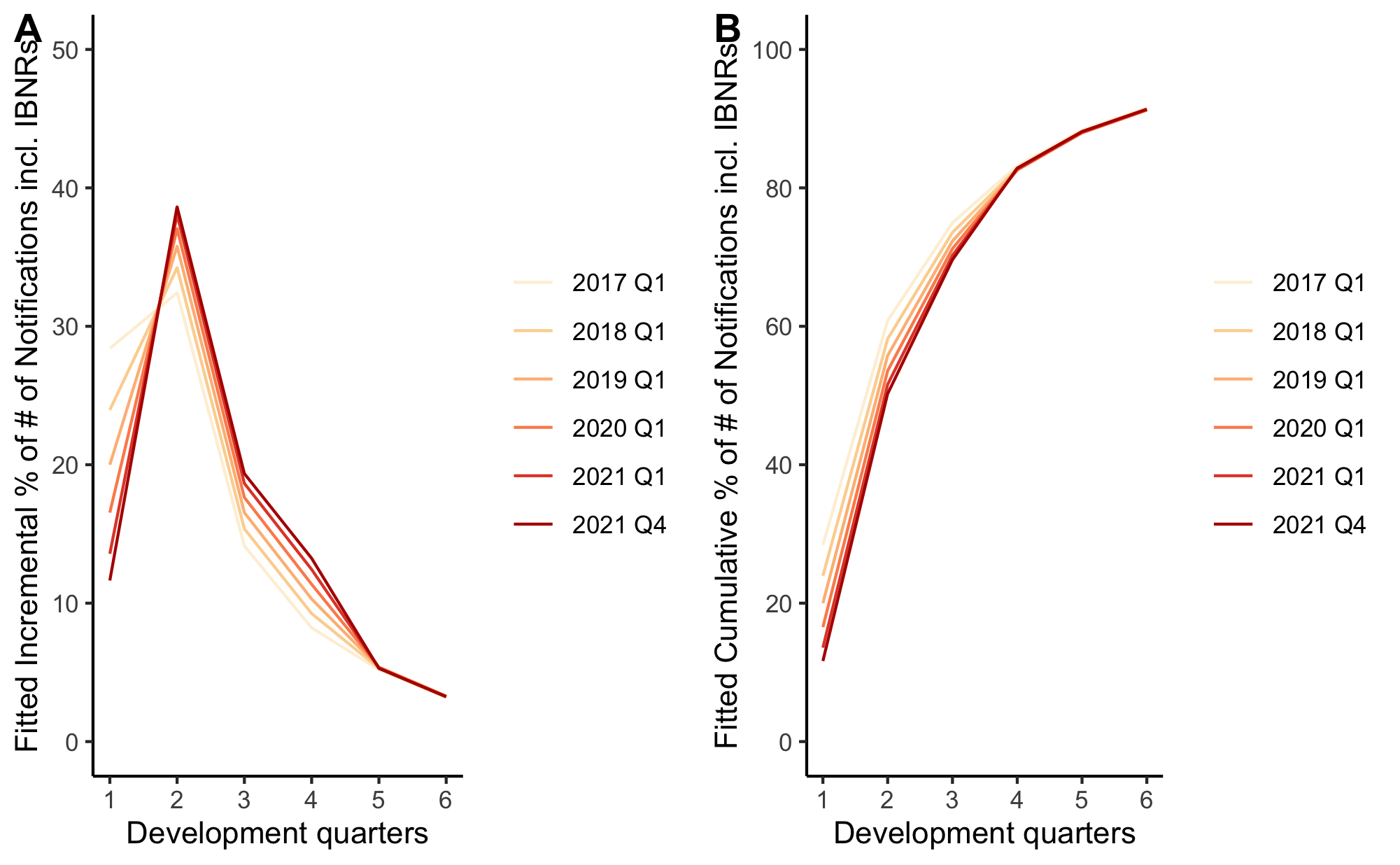
(a) AQ 2017Q1 - AQ 2021Q4, CA($>$499)

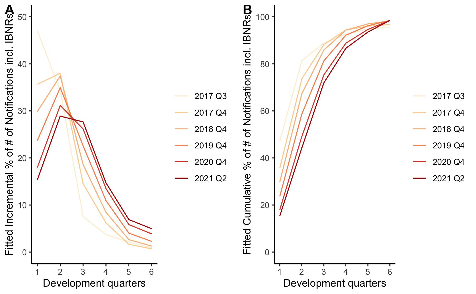
(b) AQ 2014Q1 - AQ 2021Q2, IN (0-249)

Figure 1: Development pattern trends

5.2 Accident period trend

5.2.1 The inclusion of IBNRs reveals escalating frequency

The inclusion of projected IBNRs leads to a notable rise in claim frequency across all states and severities beyond 2020, as opposed to the decrease in frequency that would be seen if actual counts were the only consideration. See Figure 2(a) for CA($>$499) and Figure 2(b) for IN(0-249), and all other major cases in Appendix E.

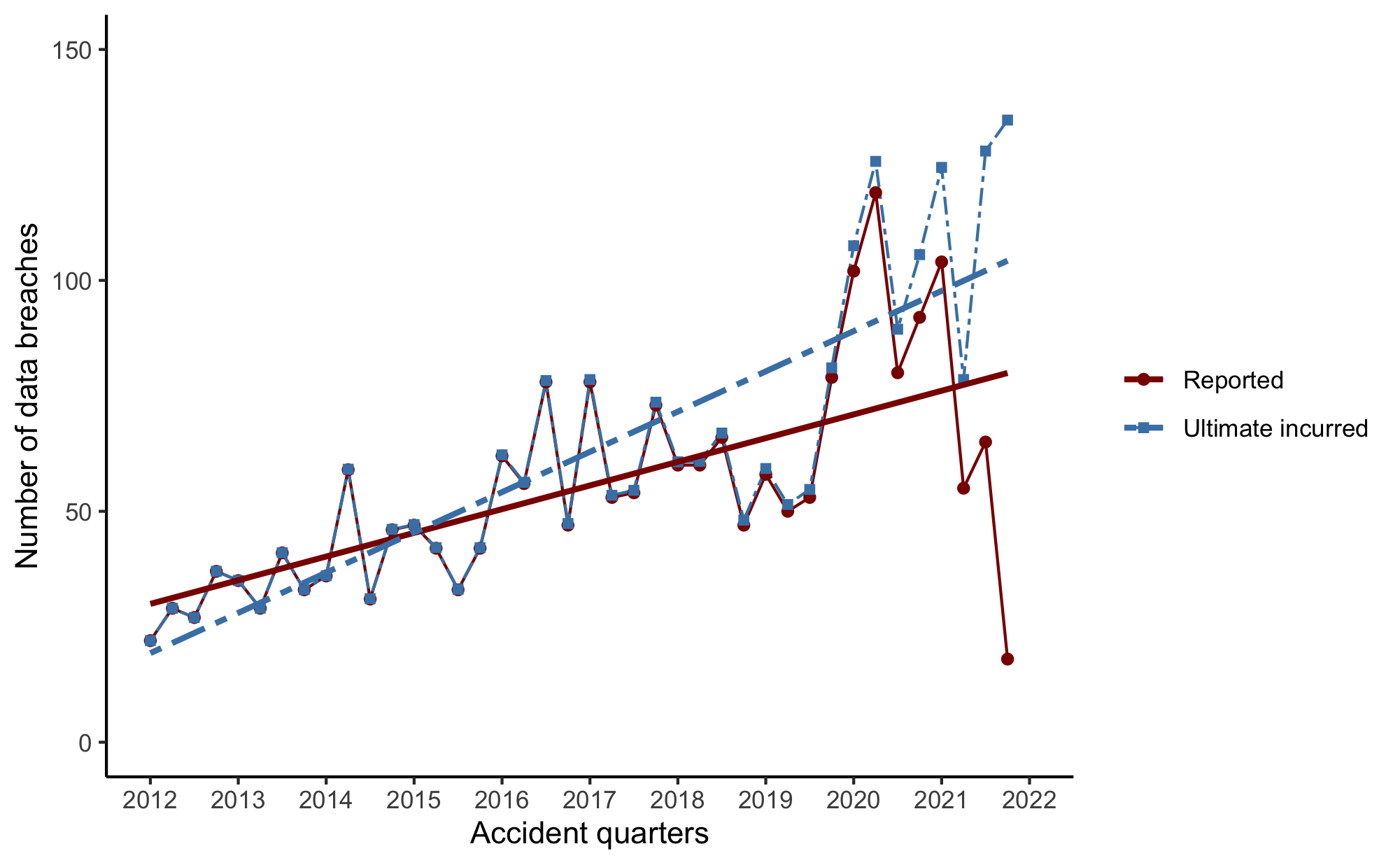
(a) AQ 2012Q1 - AQ 2021Q4, CA($>$499)

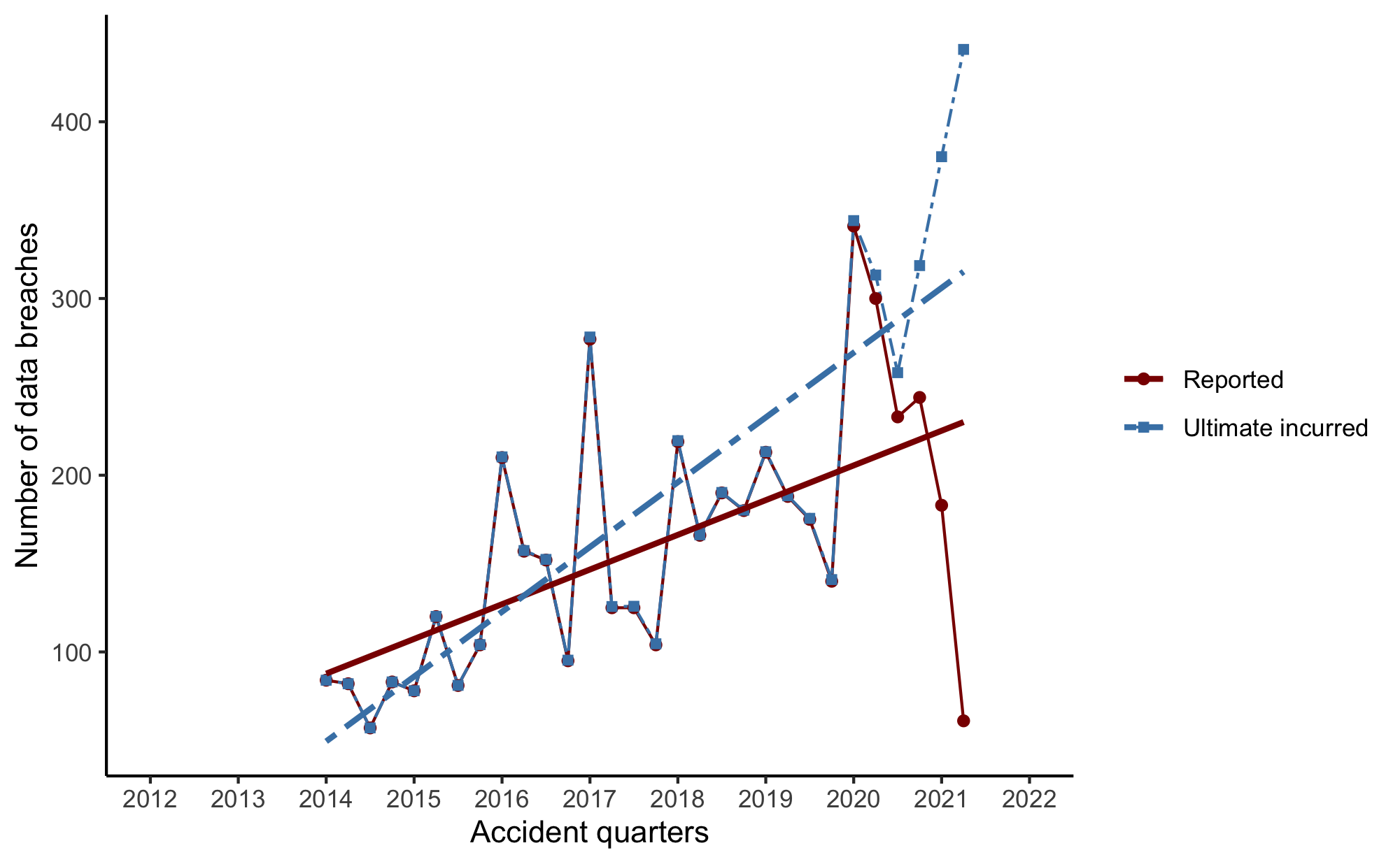
(b) AQ 2014Q1 - AQ 2021Q2, IN (0-249)

Figure 2: Reported versus Ultimate incurred breaches

5.2.2 CA, IN, MT, and ME exhibit highly similar frequency trends

The growth of quarterly ultimate incurred breaches between 2016Q1 and 2021Q4 is similar across all four states when compared to the average quarterly number of breaches between 2015Q4 and 2016Q3. See Figure 3.

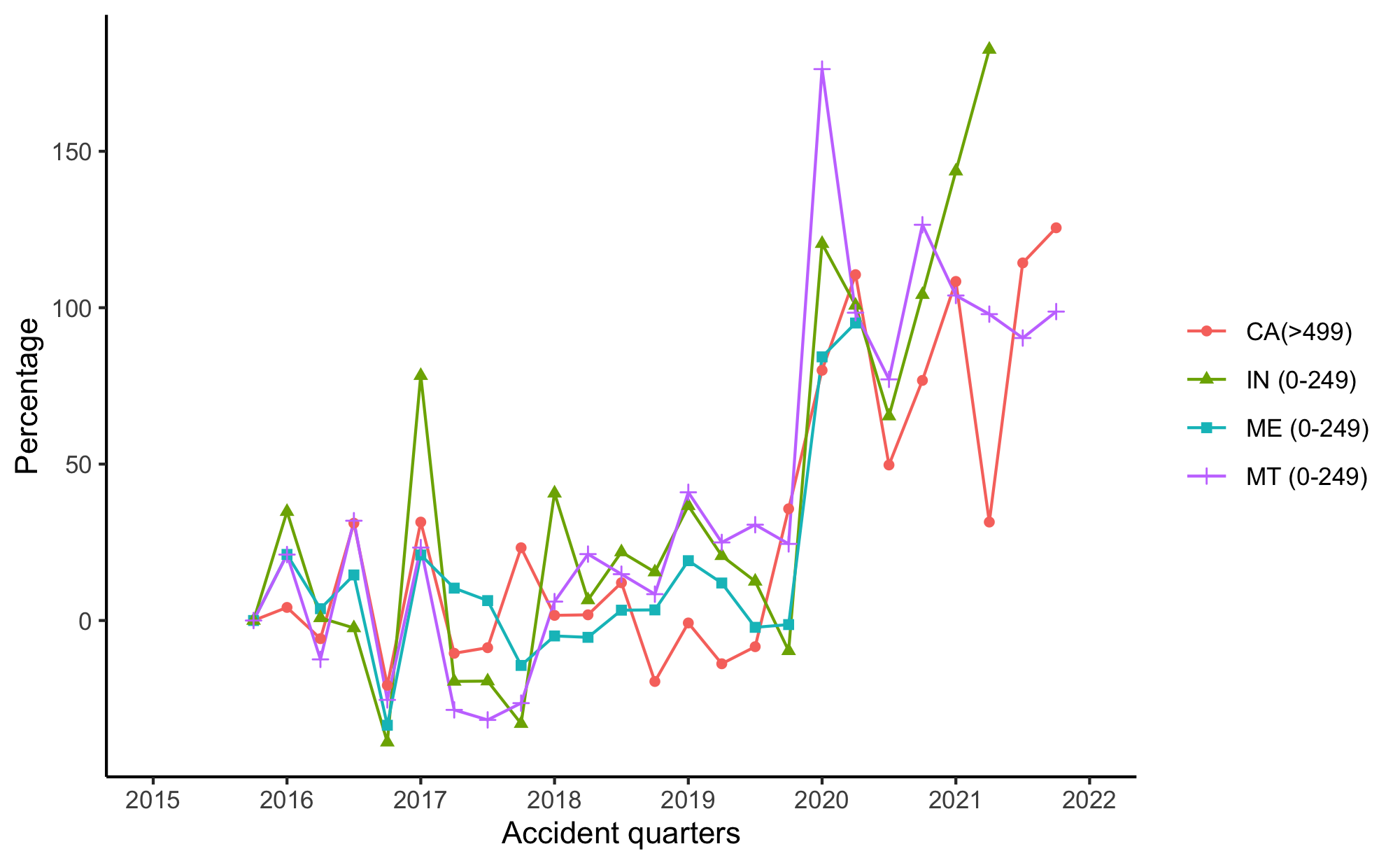
Figure 3: Ultimate incurred breaches by AQ, expressed as
a percentage of the average over AQs 2015Q4 to 2016Q3

Starting from 2014Q2, the growth rates of four states often share the same sign for the same period. Furthermore, for the periods with the highest or lowest growth rates, except for 2018Q1, the growth rates consistently maintain both sign and magnitude across states. See Figure 4.

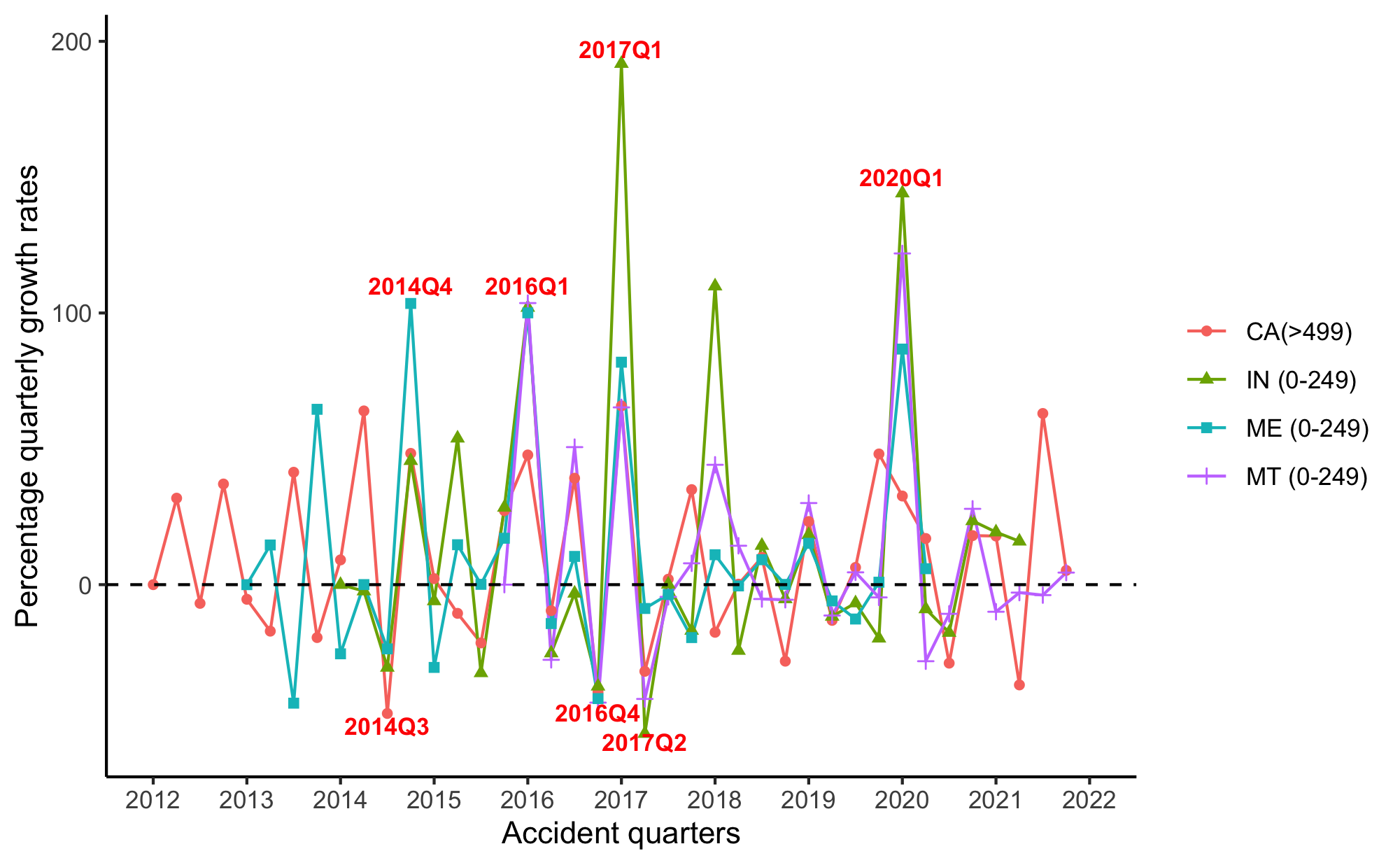
Figure 4: Quarterly growth rates of ultimate incurred breaches (AQ 2012Q1 - 2021Q4)

5.2.3 2020Q1 marks a break-point in frequency trends for all states

Equation (9) shows the forms of model tested for frequency trends in individual cases, with log of the number of notifications being the dependent variable. $\alpha_{3}$ is statistically significant in most states and severities, meaning that 2020Q1 is the break-point in their frequency trends. Below, we will discuss the differences in the frequency trends across individual cases.

$$\begin{split}\alpha_{0}+\alpha_{1}\cdot i+\alpha_{2}\cdot i^{2}+\alpha_{3}\cdot 1_{i\geq 2020Q1}(i)+\alpha_{4}\cdot 1_{2020Q1}(i)+\alpha_{5}\cdot 1_{2020Q2}(i)+\alpha_{6}\cdot\max(0,i-2020Q2)\end{split}$$ (9)

• CA($>$499), IN(0-249): $\alpha_{4}$ and $\alpha_{5}$ are insignificant, all else significant in CA($>$499). $\alpha_{4}$ is insignificant in IN(0-249). There is a sudden increase in the quarterly number of breaches in 2020Q1, followed by a continuous upward trend.

• MT(0-249), ME(0-249), WA($>$499), OR($>$250), IN($>$499), MT(250-499), ME(250-499), ND(250-499): $\alpha_{4}$, $\alpha_{5}$, $\alpha_{6}$ are insignificant. Following the spike in 2020Q1, the quarterly number of breaches stabilises at a relatively higher level.

• ND($>$499), IN(250-499): $\alpha_{5}$, $\alpha_{6}$ are insignificant. After the sharp increase in 2020Q1, the quarterly count of breaches declines to a level below that of 2020Q1, but stays elevated compared to pre-2020Q1 periods.

5.2.4 Smaller breaches show faster growth and greater volatility compared to larger breaches

IN(0-249) exhibits the highest and lowest growth rates among the four major data segments (see Figure 4).

To ensure meaningful comparisons among states with varying data availability, we calculate the mean and standard deviation of percentage quarterly growth rates based on the largest common time periods observed in two or more states. The resulting values are presented in Table 6. On average, IN(0-249) has the highest and most volatile growth rates, followed by ME(0-249) and MT(0-249), and then CA($>$499).

Table 6: Mean and standard deviation of percentage quarterly growth rates

	CA(>499)	ME(0-249)	IN(0-249)	MT(0-249)
2013Q2-2014Q1	3.47(28.40)	2.51(47.97)	NA	NA
2014Q2-2015Q4	8.90(39.66)	11.62(44.28)	8.09(35.03)	NA
2016Q1-2020Q2	10.41(30.41)	11.89(38.27)	20.36(68.48)	14.97(46.64)
2020Q3-2021Q2	-7.46(29.56)	NA	10.29(18.86)	1.07(18.24)
2021Q3-2021Q4	34.12(40.85)	NA	NA	0.29(5.87)

5.3 Interactions between development periods and accident periods

5.3.1 All states experience shifts in their reporting patterns, and the reporting patterns vary based on breach severity

Equations (10) and (11) show a subset of terms to model reporting patterns across accident periods in different states, with log of the number of notifications being the dependent variable.

$$\begin{split}\beta_{1}\cdot\ln(j+1)+\beta_{2}\cdot\ln(j+1)\cdot 1_{[1,4]}(j)+\beta_{3}\cdot\ln(j+1)\cdot 1_{[1,4]}(j)\cdot\max(0,i_{1}-i)\end{split}$$ (10)

$$\begin{split}\gamma_{1}\cdot j+\gamma_{2}\cdot\max(0,j-6)+\gamma_{3}\cdot 1_{\{1,2,5\}}(j)+\gamma_{4}\cdot 1_{\{2,5\}}(j)+\gamma_{5}\cdot 1_{\{5\}}(j)+\gamma_{6}\cdot\max(0,j-6)\cdot\max(0,i-i_{2})\end{split}$$ (11)

For larger breaches (see equation (10)), in the case of CA($>$499), the number of notifications declines as a power function of DQ, with different exponents before and after DQ 4. In addition, the before-DQ-4 exponent varies with AQ, indicating that the short-term notification profile has varied with AQ. See Figure 1(a) for the trends in the notification profile between 2017Q1 and 2021Q4. For detailed descriptions of the changes in trends across all AQs, see Appendix F.1.

For smaller breaches (see equation (11)), IN(0-249), MT(0-249), and ME(0-249) share another type of reporting pattern. The number of notifications decreases exponentially with change in decay factor at DQ 6, and corrections at DQ 1, 2, and 5. The decay factors used to model the notification profile also vary with AQ. See Figure 1(b) for the trend in the notification profile of IN(0-249). See Appendix F.2 to F.4 for descriptions of the changes in trends of IN(0-249), MT(0-249), and ME(0-249).

5.3.2 Around 2017, all states observe a shift in their reporting patterns

After some point in 2017, all states observe a different trend in their reporting patterns. One of the two change-points in the reporting pattern of CA($>$499) is 2017Q1 (see Appendix F.1). IN(0-249), MT(0-249), and ME(0-249) experience relatively constant reporting patterns before and including 2017Q3, and shift away from them since 2017Q4 (see Appendix F.2 to F.4).

5.3.3 The reporting delay has been getting longer in most states

Figure 5(a) - 5(b), and Appendix G compare the fitted average delay and its trend (i.e., assume no calendar period effects and exceptional observations) for the four major cases. For periods that have been assigned zero weight (see notes at the bottom of Table LABEL:tab:glm_mean), the figure compares the actual delay observed in the data and the trend.

The average delays of CA($>$499), IN(0-249), and ME(0-249) have lengthened to different extents after 2017 compared to prior periods. The average delay of MT(0-249) has decreased slightly, but not significantly compared to previous periods.

CA($>$499)

Shown in Figure 5(a), the average time to report data breaches is 2.8 quarters in AQ 2012Q1, increases to 3.2 quarters in AQ 2014Q3, decreases slightly to 3.1 quarters in AQ 2017Q1, and increases again to 3.4 quarters in AQ 2021Q4. It takes 2 quarters to reach 65$\%$ of reporting in AQ 2012Q1, but takes 3 quarters in AQ 2021Q4 (see Appendix F.1).

IN(0-249)

Shown in Figure 5(b), the average time to report data breaches is 2.2 quarters between AQ 2014Q1 and AQ 2017Q3, and increases to 2.9 quarters in AQ 2021Q2. It takes 2 quarters to reach 80$\%$ of reporting between AQ 2014Q1 and AQ 2017Q3, but takes 4 quarters in AQ 2021Q2 (see Appendix F.2).

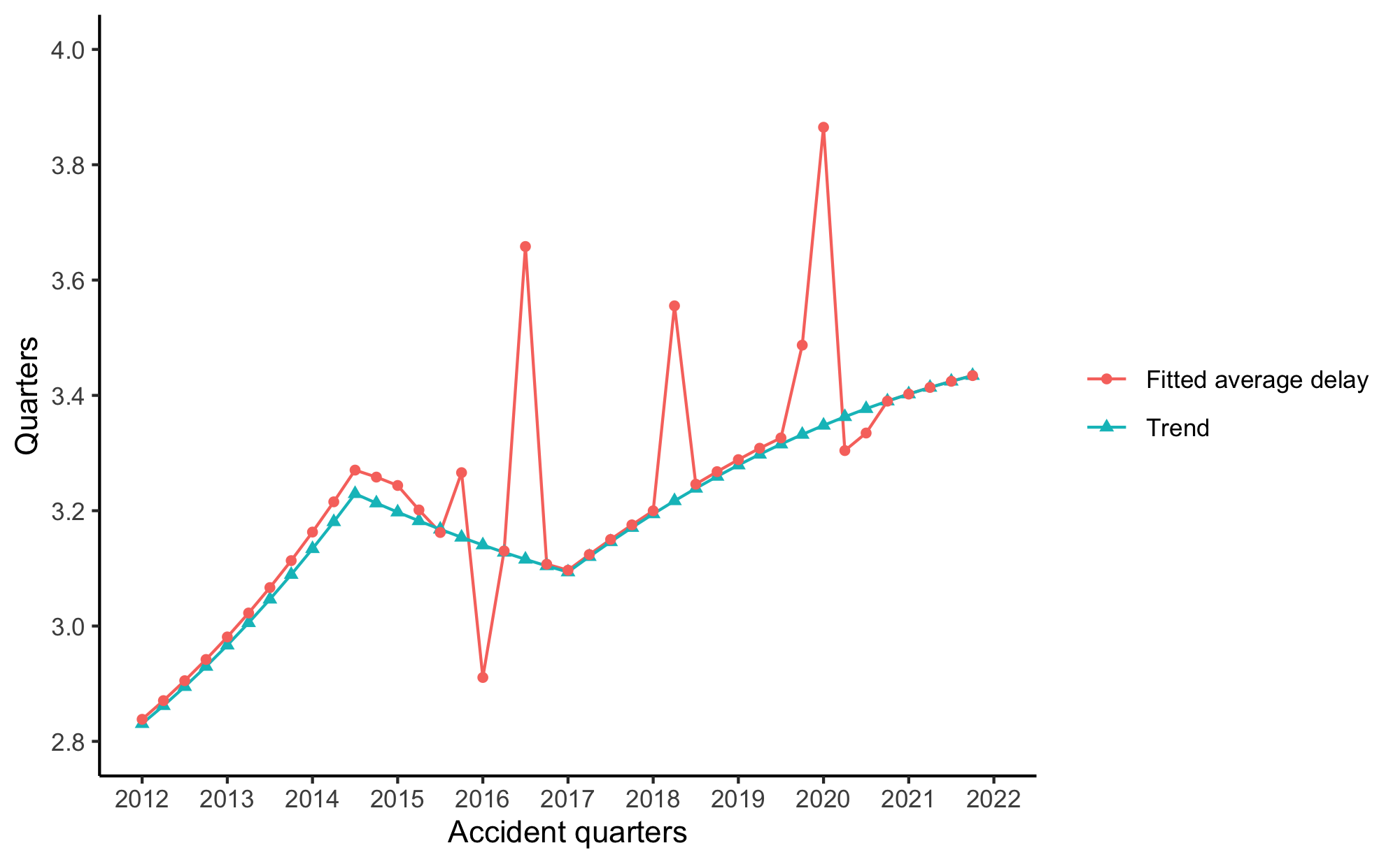
(a) CA($>$499)

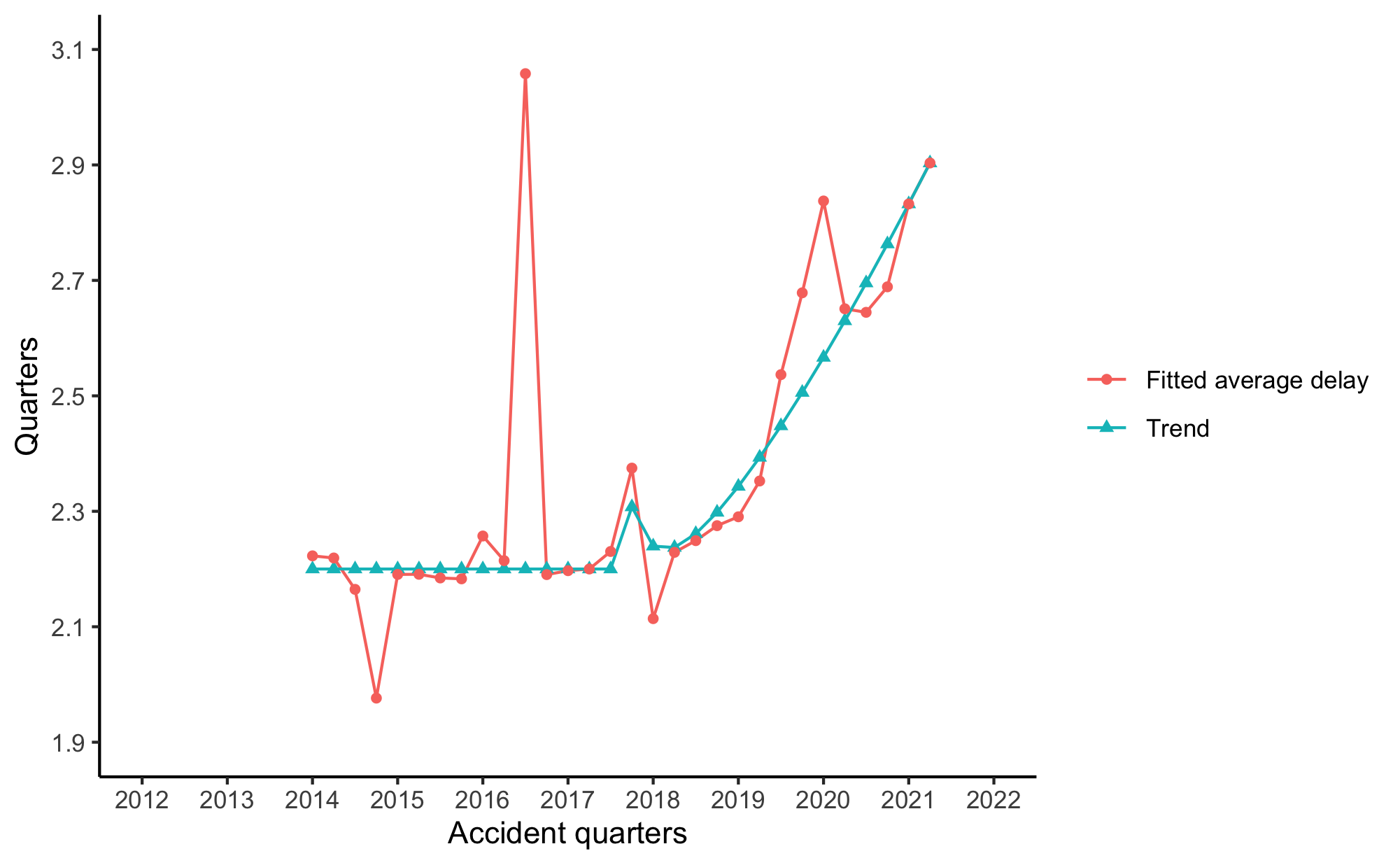
(b) IN(0-249)

Figure 5: Fitted average delay and its trend

5.3.4 The reporting of data breaches shifts away from the first quarter of occurrence across all states

The percentage of breaches that are reported within the quarter of their occurrence has decreased across all states, regardless of whether the average delay has improved or gotten worse (see Appendix F). On average, it has decreased from more than 30$\%$ in 2017 to less than 15$\%$ in 2021.

For example, MT(0-249) is the only state that has seen a slight improvement in the average reporting delay after 2017 (see Figure 6(b)). However, just like the other states with deteriorating reporting delay, the percentage of notifications received in the quarter of breach occurrence has decreased from 35$\%$ in 2017Q3 to 12$\%$ in 2021Q4, shown in Figure 6(a).

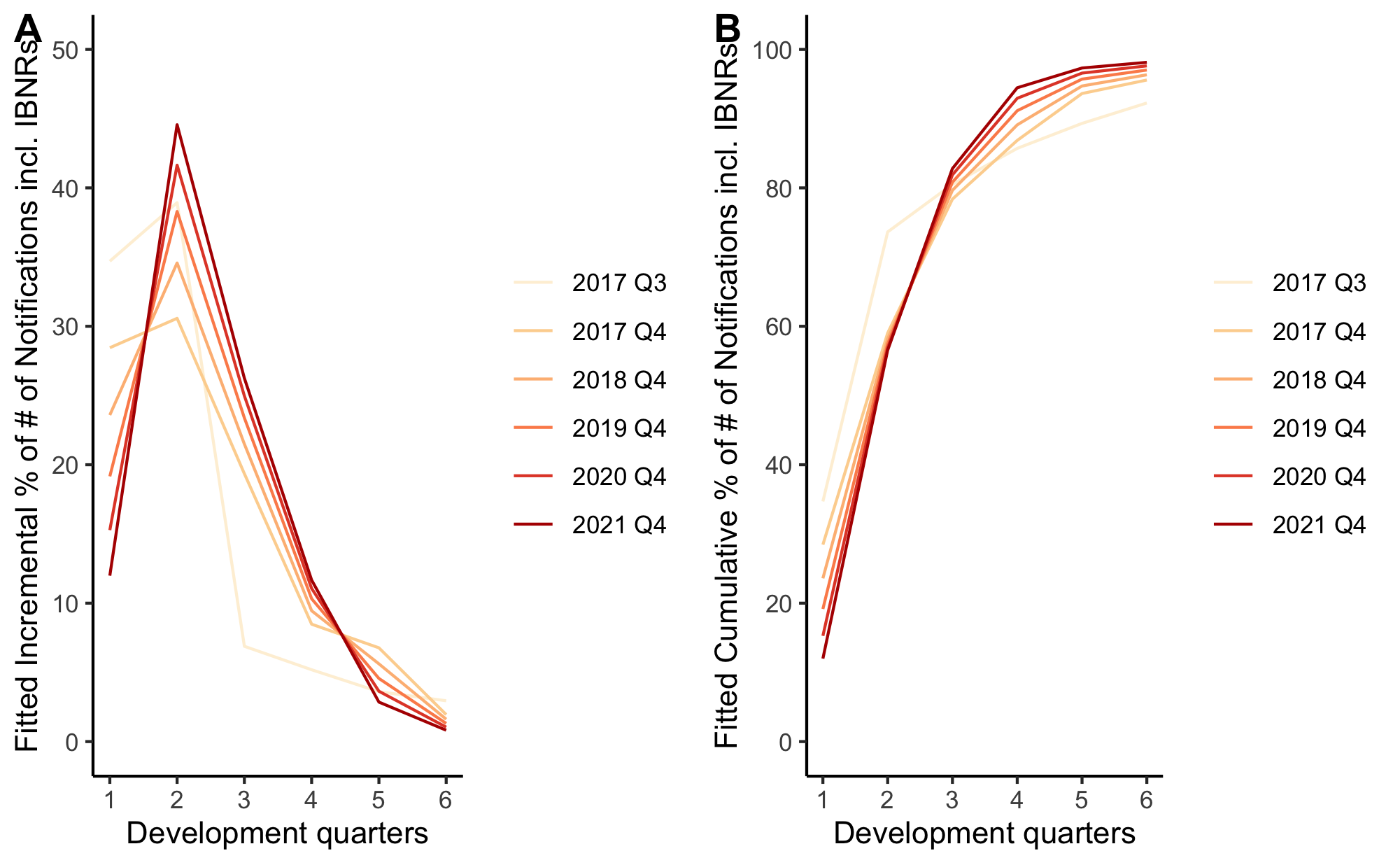
(a) Development pattern trend

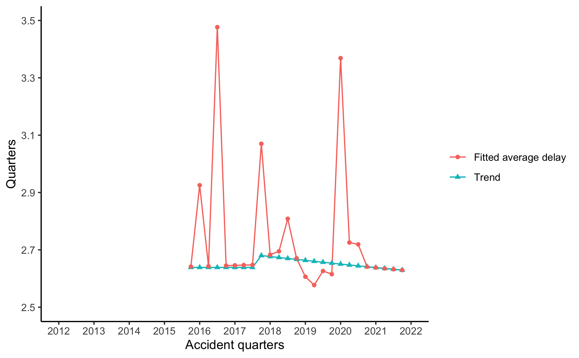
(b) Fitted average delay and its trend

Figure 6: AQ 2015Q4 - AQ 2021Q4, MT (0-249)

5.4 Exceptional observations

5.4.1 Some periods of erratically long reporting delay are shared across all states

During three periods (AQ 2016Q1, AQ 2016Q3, and AQ 2020Q1), all states have experienced significant delays in reporting breaches. These are isolated changes that are significantly off-trend. In addition to the four major cases, we also observe them in WA($>$499), OR($>$249) and IN($>$499).

We see the most drastic change, in the average delay of breaches occurred for each of these periods, in MT(0-249) (see Table 7). Table 7 shares the same statistics with Figure 5(a) - 5(b), and Appendix G. See Section 5.3.3 for how we compute these statistics. Although there is no evidence of sustained change of the reporting pattern in MT(0-249), MT(0-249) is subject to the greatest volatility in the average reporting delay across accident periods (see Appendix F.3).

In AQ 2016Q3 and AQ 2020Q1, all states are subject to extended reporting delays. For example, in AQ 2020Q1, the average delay in MT(0-249) increases to 3.4 quarters, which would otherwise be 2.6 quarters. IN(0-249) is up by 0.3 quarters to 2.9, from 2.6 quarters. For larger breaches, in CA($>$499), the average delay increases to 3.9 quarters, which would have been 3.4 quarters. The delay experience in AQ 2020Q1 is exceptional compared to other AQs for IN(0-249), MT(0-249), CA($>$499), and WA($>$499); to avoid the distorting effects of such experience, we assign zero weight to it in the modelling.

In AQ 2016Q1, almost all states are subject to longer-than-usual reporting delays, except that CA($>$499) has shorter-than-usual delay. CA($>$499) experiences extra-long average delay in AQ 2015Q4. It is also worth noting that WA($>$499) and OR($>$249) have also experienced longer delay (see Appendix B). We assign zero weight to the entire AQ 2016Q1 in the modelling of these two states.

CA($>$499) and IN(0-249), both of which experience non-trivial lengthening reporting delays after 2017, also see longer-than-usual delays in AQ 2019Q4. See Figure 5(a) and 5(b).

Table 7: Average delay in quarters - pre and aft accounting for exceptions

	2016Q1	2016Q3	2020Q1
CA(>499)	3.1 $\rightarrow$ 2.9	3.1 $\rightarrow$ 3.7	3.4 $\rightarrow$ 3.9
IN(0-249)	2.2 $\rightarrow$ 2.3	2.2 $\rightarrow$ 3.1	2.6 $\rightarrow$ 2.9
MT(0-249)	2.6 $\rightarrow$ 2.9	2.6 $\rightarrow$ 3.5	2.6 $\rightarrow$ 3.4
ME(0-249)	2.4 $\rightarrow$ 2.5	2.4 $\rightarrow$ 3.2	NA

5.4.2 An increase in notifications at DQ 4 or DQ 5 is noted during periods of extended reporting delay

During periods of extended reporting delay, most of the time, we observe a spike in notifications at DQ 4 or DQ 5, which is at least higher than the number of breaches reported at DQ 3.

Appendix B show the actual quarterly triangles in all data segments. Among breaches occurred in 2016Q3, the number of notifications at DQ 5, in all four major cases and also IN($>$499), is equivalent to or even higher than any other DQs in the same AQ. Among breaches occurred in 2015Q4 of CA($>$499), the number of notifications at DQ 4 is close to the highest. Among breaches occurred in 2016Q1, IN(0-249), MT(0-249), ME(0-249), and IN($>$499) see a spike of notifications at DQ 5.

5.5 Calendar period effects

5.5.1 Opposite calendar period effects in adjacent periods

A higher/lower total number of notifications received by the state Attorney General in a CQ is compensated by a lower/higher number in the next CQ, observed in IN(0-249) and ME(0-249). This often results in a period of longer-than-usual delay followed by shorter-than-usual delay, when speaking to accident periods, and vice versa.

IN(0-249)

The number of notifications received in CQ 2017Q4 is 24$\%$ lower than what is modelled in the absence of CQ effects, whereas the number of notifications in CQ 2018Q1 is 31$\%$ higher. Consequently, breaches occurred in 2017Q4 has longer-than-usual delay, followed by 2018Q1 shorter-than-usual delay (see Figure 5(b)).

ME(0-249)

The number of notifications received in CQ 2018Q2 is 27$\%$ higher than what is modelled in the absence of CQ effects, whereas the number of notifications in CQ 2018Q3 is 21$\%$ lower. The number of notifications received in CQ 2018Q4 is 29$\%$ lower than what is modelled in the absence of CQ effects, whereas the number of notifications in CQ 2019Q1 is 41$\%$ higher. As a result, breaches occurred in 2018Q1 has shorter-than-usual delay, followed by 2018Q3 longer-than-usual delay, and 2019Q1 shorter-than-usual delay.

5.6 Residual model effects

Item 1: For the 11 less numerous cases (e.g., IN($>$499)), we find some similarities between their development patterns. The general structure of their development patterns is represented by equation (12), where $\alpha_{i}$ represents the accident period effects (abbreviated as such), and interactions are not explicitly shown in order to maintain focus.

$$\begin{split}\ln(u_{ij})&=\alpha_{i}+\gamma_{1}\cdot j+\gamma_{2}\cdot\max(0,j-6)+\gamma_{3}\cdot 1_{\{1,2,5\}}(j)+\gamma_{4}\cdot 1_{\{2,5\}}(j)+\gamma_{5}\cdot 1_{\{5\}}(j)\end{split}$$ (12)

The development pattern amounts to an exponential curve with change in decay factor at DQ 6, and corrections at DQ 1, 2, 5. Some might share a common set of coefficients, while others might have identical coefficients for the exponential curves (i.e., $\gamma_{1}$, $\gamma_{2}$) or the corrections (i.e., $\gamma_{3}$…$\gamma_{5}$). See the former presented by Term 8 - 10 in Table LABEL:tab:glm_mean, and the later presented by Term 1 - 7.

When two data segments share the same $\gamma_{3}$, it indicates that the DQ coefficient at $j=1$ in the two segments may be significantly different, but the difference between that coefficient and the coefficients of their respective exponential curves may not be. A common $\gamma_{4}$ suggests that the difference between the coefficients at $j=2$ and $j=1$ is identical, and a common $\gamma_{5}$ suggests that the difference between the coefficients at $j=5$ and $j=2$ is identical.

Item 2: To characterise accident period effects, we have trend terms and indicator functions to correct for certain anomalies. For example, in equation (13) where $\beta_{j}$ is abbreviated for development period effects, there is a quadratic trend and two indicator functions to address poor fit of two periods.

In some instances, we find that the deviation from the general accident period trend across periods is similar in a single data segment (i.e., similar $\alpha_{3}$ and $\alpha_{4}$). See Term 19 - 22.

Sometimes, different data segments may show a similar deviation from their respective accident period trends in the same period or different periods. This means some segments might have a common $\alpha_{3}$ or the $\alpha_{3}$ in one segment is similar to the $\alpha_{4}$ in another segment. See Term 11 - 13. However, it is worth noting that these data segments may not necessarily have the same accident period trend.

$$\begin{split}\ln(u_{ij})&=\beta_{j}+\alpha_{1}\cdot i+\alpha_{2}\cdot i^{2}+\alpha_{3}\cdot 1_{i_{1}}(i)+\alpha_{4}\cdot 1_{i_{2}}(i)\end{split}$$ (13)

Item 3: We observe similar calendar period effects across different periods in a single data segment and in the same period across adjacent data segments. In equation (14), $\phi_{1}$ and $\phi_{2}$ are similar in WA($>$499) for CQs 2017Q2 and 2018Q4. A common $\phi_{2}$ is shared across WA($>$499) and OR($>$249) for CQ 2018Q4, although they do not have the same accident period trend and development pattern. See Term 14.

$$\begin{split}\ln(u_{ij})&=\alpha_{i}+\beta_{j}+\phi_{1}\cdot 1_{c_{1}}(c)+\phi_{2}\cdot 1_{c_{2}}(c)\end{split}$$ (14)

Item 4: When correcting for exceptional cells, we find that sometimes the correction is similar across multiple exceptional cells in a single data segment (i.e., similar $\phi_{1}$ and $\phi_{2}$ in equation (15)). Sometimes, the correction for the same exceptional cell is identical across multiple data segments, indicated by a common $\phi_{1}$. For example, IN($>$499) has the same correction for (DQ 5, AQ 2016Q1), (DQ 5, AQ 2016Q3), and (DQ 5, AQ 2017Q4); the correction for (DQ 5, AQ 2016Q3) is similar among IN($>$499), WA($>$499), and OR($>$249). See Term 23 and 24.

$$\begin{split}\ln(u_{ij})&=\alpha_{i}+\beta_{j}+\phi_{1}\cdot 1_{i_{1}}(i)\cdot 1_{j_{1}}(j)+\phi_{2}\cdot 1_{i_{2}}(i)\cdot 1_{j_{2}}(j)\end{split}$$ (15)

5.7 Limitations

Our analysis presents some limitations. First, despite the fact that we attempted to employ an event definition that takes into account both the third-party provider and all of its affected client firms in the event of a third-party data breach, we only included businesses that met state notification requirements due to data limitations. Second, the conclusions on data breach notifications and frequency trends were drawn based on a subset of state Attorneys General’s data that explicitly provides dates of occurrence and dates of notification. Data breaches in other states may display distinct features. Third, we did not incorporate a national analysis, due to the lack of data. When more data are available, it would be interesting to perform multi-state analysis on breaches with the same definition, after filtering out common breaches across states. Fourth, it is unclear whether the lengthening delay between occurrence and reporting is the result of a lengthening delay between occurrence and discovery, between discovery and reporting, or both. This ambiguity arises because most states do not explicitly provide dates of discovery. By extracting discovery dates from breach notices, it may be possible to conduct additional research into the causes of lengthening delay. Fifth, it is unknown whether similarities among states in breach experience are the result of a high proportion of third-party data breaches or of breaches affecting residents of multiple states. This could be investigated further by identifying third-party breaches via breach notice letters and identifying breaches that affect residents of multiple states by identifying common breaches across states.

6 Insights and implications

This section summarises the main research findings, with a particular emphasis on examining the insurance implications of the main model output presented in Section 5. Through this analysis, we offer valuable insights into a variety of insurance-related issues, including pricing, reserving, underwriting, and capital needs.

First, we present an initial attempt to more accurately assess the frequency of both historical and recent data breach risks in the United States, by taking into account some peculiarities when analysing actual event data. Section 6.1 highlights key data considerations for informing data breach risk evolution from incident data that are discussed in Section 2.

Second, we analyse the delay between the occurrence of a data breach and the reporting to state regulators, and examine the frequency of data breaches. By focusing on the intricate details of the data in the model, we unearth characteristics that have not been previously discussed in the literature. Having knowledge of these features, including similarities in breaches with the same severity across different states, is extremely valuable when it comes to pricing, reserving, and gaining a general understanding of how cyber incidents are evolving. As cyber risks evolve quickly, we should carefully evaluate and consider the implications of these characteristics to make informed decisions. Section 6.2 commences with a concise overview of the data usage and methodology utilised in this study. The section then highlights the key results from the modelling that were uncovered in Section 5, followed by an explanation of their potential implications for insurance. Table 8 summarises key results and their implications.

6.1 Data analysis considerations

6.1.1 A different event definition to assess the actual impact of data breaches

One of the peculiarities of cyber risk is that event definition can be complicated by interdependencies among certain security incidents (Wheatley et al., 2021), namely third-party cyber events. A third-party cyber event can be considered as 1) a single event occurred at the third-party provider or one of its affected client firms, or 2) a series of correlated events at the provider and all of its affected client firms. In this paper, we adopt the latter definition for third-party data breaches, which is necessary from both economic and cyber insurance perspectives. Reasons are briefly explained below (more details in Section 2.2.2).

To avoid underestimating the risk of a data breach, a third-party data breach should be viewed as a series of events (the second definition defined above). If not, we would underestimate the total number of businesses that are affected by such a breach, resulting in an overall underestimation of the frequency rate. Second, we would underestimate the economic impact of the third-party data breach, by failing to account for the impact on each of all affected businesses. Third, we would underestimate the dependencies across organisations because the data do not capture the dependence resulting from the utilisation of common services and providers.

Cyber insurers should also consider a third-party data breach as a series of events to assess its impact on a cyber portfolio. In the event of a third-party data breach, when a cyber insurer insures both the third-party provider and its client firms, the insurer may face multiple claims. Viewing this breach as a single event may lead to underestimation of the frequency and severity of such breaches, as well as the dependencies between insureds in the portfolio, for the same reasons as stated previously. As a result, the insurer would undervalue the aggregate pricing of the portfolio. Therefore, in order to reflect the actual position of the insurer, this data breach should be regarded as a group of dependent events.

As this type of data breach becomes more prevalent than ever before, the definition and modelling of its frequency and severity will greatly affect the overall estimation of data breach risk, both at the societal level and from the perspective of a cyber insurer. Therefore, they should be carefully considered. The IBM Cost of a Data Breach Report 2022 states that 19$\%$ of breaches occurred because of a compromise at a business partner (IBM, 2022).

6.1.2 Frequency trend uncovered by controlling for changes in the reporting propensity

We uncover the frequency trend following an attempt to circumvent the limitation of changing propensity of organisations to report data breaches across periods, hence aiding in the estimation of the true frequency distribution of actual breach occurrences.

Constant reporting means that the reporting propensity of occurred data breaches does not vary between time periods (see the definition of reporting propensity in Section 1). If the reporting propensity remains constant over occurrence periods, then counts of reported events will vary proportionately with those incurred, and the former will validly reflect any trend in the latter.

There have likely been changes in the propensity to report data breaches that are of varying severities in the U.S., as a result of differing state laws governing data breach notification obligations and the evolution of such requirements over time within individual states (more details in Section 2.2.3). Therefore, to unravel the frequency trend, we segregate data breaches by the state laws to which they are subject, and only analyse breaches of selected time periods, whereas most current literature that studies data breaches in the U.S. performs national analysis across all available time periods. Then, we have no reason to believe that the reporting propensity of the data breaches under investigation has varied, and assume it constant for the purpose of this paper. Below, we provide a brief summary of the two main reasons why the reporting propensity might have materially changed and the selection of data breaches due to this consideration.

First, the number of entities that must be notified of a breach has expanded, to include government bodies such as state Attorneys General, which may have led to a greater number of breaches being made public after this change. To overcome the change in the reporting propensity caused by this, we analyse data breaches made available directly by individual state Attorneys General, which are those occurred after mandatory notification of the respective Attorney General.

In addition, states enact the requirement to notify the state Attorney General of certain breaches at different times, which creates challenges for a sound national analysis due to changing reporting propensity over time at the national level. Therefore, to determine the evolution of data breach risk over time, we perform an analysis over states that provide relevant data and differentiate states within the model to the extent that is needed.

Second, states have different definitions of what constitutes a data breach that must be reported to government authorities. In particular, the number of affected state residents above which notifying the respective state Attorney General is required varies by state. This may have resulted in state-by-state variations in the reporting propensity of data breaches with varying severities. Consequently, when comparing across states, we should compare data breaches that are subject to the same definition, as is done in this paper.

6.2 Key insights from numerical analysis and their implications

To unravel the evolution of data breach risk over time, we investigate data breaches at state levels which are made available directly by state Attorneys General, and compare data breaches that are subject to similar definitions, as explained above. As many cyber insurers need to quantify their liabilities quarterly (see Section 3.4), we aggregate data breaches quarterly for analysis.

In particular, we investigate eight state Attorneys General publications of data breaches, out of 17. This is because they report breach incidence dates, which allows investigation of data breach reporting patterns and thus helps yield a more complete picture of recent data breach trends after reasonable estimation of IBNR breaches. They are California, Delaware, Indiana, Maine, Montana, North Dakota, Oregon, and Washington state.

We conduct two-dimensional analyses of data breach frequency data, namely the change of reporting delay and the trend of data breaches between 2012 and 2021 simultaneously by applying GAMs to ODP observations based on run-off triangles. To create a comprehensive model, we first develop a GAM for each state and severity. Subsequently, we utilise the common characteristics among states and severities to merge these individual models into a single model. Projecting IBNR breaches involves extrapolating historical development profiles to the future, and the projected IBNR breaches are then added to the reported breaches to reveal the frequency trends.

Our findings and their implications are explained in the following subsections, and summarised in Table 8 at the end of this section.

6.2.1 Lengthening delay between data breach occurrence and reporting

Result 1: The average delay of data breaches, between the first possible date of breach occurrence and the date reported to government bodies, has lengthened to different extents after 2017 compared to prior periods in California, Indiana, and Maine. For example, for breaches that affect more than 500 California residents, it takes two quarters to reach a reporting rate of $65\%$ for breaches that occurred in 2012Q1, but it takes three quarters for breaches that occurred in 2021Q4.

Insight 1.1: If the lengthening delay between occurrence and reporting is the result of a lengthening delay between discovery and reporting, cyber attacks that result in data breaches are becoming more effective and costly.

In cyber security terminology, the time to detect a breach is referred to as dwell time, the period of time between a cyberattacker’s entry and removal from a system (Security Boulevard, 2022). Cybercriminals are surreptitious and persistent, frequently operating invisibly on a network for weeks or even months at a time. Long dwell times provide cybercriminals more time to understand the network architecture, the access they have through stolen credentials, and the location of sensitive data (SecurityBrief Australia, 2021). Consequently, they are given more opportunity to access personally identifiable information, compromise financial accounts, and insert malicious malware through newer and more sophisticated attacks.

Longer intruder dwell times continue to associate with greater potential impact of a data breach, a finding noted by IBM since 2016 (IBM, 2022). In 2022, the average cost of a data breach with an average time to identify and contain of fewer than 200 days was USD 3.74 million, while the cost of breaches with an average time of more than 200 days was USD 4.86 million. For breaches with a shorter than 200-day lifespan, this difference provides an average cost reduction of USD 1.12 million, or 26.5$\%$.

Insight 1.2: Cyber insurers are less certain of the risk assumed at the underwriting stage, in terms of whether the potential insured has already been compromised.

Cyber insurance policy can be written on an occurrence basis or on a discovery basis. On an occurrence basis, the policy will cover insured events that occur during the policy period. On a discovery basis, the policy will cover events that are discovered during the policy period.

The increase in dwell times suggests that enterprises are having a more difficult time spotting threats within their increasingly complex and hybrid networks (Live Action, 2022). For covers that are provided on a discovery basis, such as those on the market, this means that when insurers write the policy, there is greater uncertainty regarding whether or not attackers have already lingered on the network. If this is the case, the organisation’s likelihood of being attacked increases, thereby increasing the insurer’s potential liability.

Insight 1.3: For policies that are provided on a discovery basis, cyber insurers should more thoroughly assess the historical attack probability of the insured.

For policies on a discovery basis, longer dwell time means that cyber insurers might be liable for hacks that are dated back longer, if they could not be detected until after policy commencement. For example, the insurer is responsible for a data breach that occurred a year ago, provided the breach is discovered after the policy takes effect. Therefore, at the underwriting stage, cyber insurers should conduct a more comprehensive assessment of a potential policyholder’s historical security position, to ensure the premiums charged reflect the underwritten risk. For example, an organisation that implemented multi-factor authentication one month ago should be rated differently than one that did so one year ago, due to the increased likelihood of incurring an attack that remains undetected.

Insight 1.4: Cyber insurers should direct more efforts towards forecasting the financial coverage of incurred but not reported (IBNR) data breach claims.

A greater proportion of data breach claims is expected to be reported in later quarters. As cyber insurers are required to report their financial condition on a quarterly basis, the need to estimate data breach claims that have been incurred but not reported (IBNR) has increased.

6.2.2 The reporting patterns of data breaches shift over time and differ by size of the breach

Result 2: Larger breaches have longer delay between occurrence and notification than smaller breaches. This is in line with the findings of the IBM Cost of a Data Breach Report 2022 (IBM, 2022).

Insight 2.1: Loss reserving should differentiate among breaches with varying severities.

As data breach reporting patterns significantly differ by severity of the breach, the severity of breaches should be factored into reserving.

Result 3: The reporting patterns of data breaches with various severities have shifted over time. The percentage of breaches reported in each of development quarters 1-6 varies by time periods. For example, an important finding is that the percentage of breaches that are reported within the quarter of their occurrence has decreased from more than 30$\%$ in 2017 to less than 15$\%$ in 2021, across all states.

Insight 3.1: Basic Chain Ladder method of reserving should not be used to predict IBNR breaches, as it will lead to inaccurate forecasting.

There is substantial evidence of shifting reporting patterns across all investigated states and breaches with different severities, which contradicts the assumption of the basic Chain Ladder method of reserving. Using basic Chain Ladder will lead to inaccurate forecasting.

Result 4: Sometimes, the reporting delay is unusually lengthy. In such instances, we observe a spike in the reporting of breaches in the fourth and fifth quarters after their occurrence, which can represent as much as 25$\%$ of the total number of breaches of the relevant accident quarter.

Insight 4.1: Cyber insurers need more capital for policies that are provided on a discovery basis, due to increased loss reserve uncertainty resulting from greater variations of reporting delay.

Due to increased variations of reporting delay across periods, suggested by Result 3 and 4, the number of eligible data breach claims may deviate from the estimated to a greater extent across different accident periods, for policies on a discovery basis. This increases the need for capital, which would occur naturally in any system where capital requirements depend on estimated forecast uncertainty (e.g., U.S., Europe, Australia).

Insight 4.2: Cyber insurers may have an estimation of the number of data breaches that will occur in each time period. If the received is lower than expected in early development quarters, cyber insurers should not assume a favourable position, as there is a possibility that the number of reported data breaches will spike in later development quarters.

Occasionally, a significant proportion of data breaches that are attributed to the same accident period might be reported in later development quarters. Consequently, even if insurers observe lower-than-usual number of claims in the first three development quarters, they are still uncertain about the ultimate liability, and have to wait until later.

6.2.3 Shared data breach experience among states

Result 5: States observe similarities in breach frequency trends, the timing of change in reporting patterns, and trends in the average delay between occurrence and reporting. Different states follow highly similar frequency trends, relatively stationary up to accident quarter 2020Q1 and increasing subsequently. The historical change in reporting pattern commences at a similar point in time across states, around 2017. All states have shown no sign of decreasing average delay between occurrence and reporting, and most have experienced lengthening delay.

Insight 5.1: There are three potential causes of commonalities among states, and none of them are encouraging.

Reason 1: One possible reason might be that a significant proportion of breaches are those that impact residents of multiple states. State Attorneys General are concerned about breaches that affect residents of their state. As a result, if a breach affects people in more than one state, the affected organisation must submit a separate report to each state Attorney General of the affected states regarding this breach. When this kind of breach accounts for a sizable fraction of the total, there is considerable overlap of breaches across states. Then, we would anticipate similarities among states. This means that a substantial percentage of breaches incurs the cost of complying with regulations in multiple jurisdictions, which is more expensive than complying with regulations in a single jurisdiction.

Reason 2: Another reason might be that a sizable portion of breaches are third-party breaches. In the event of a third-party data breach, as defined in Section 1, both the third-party vendor and its affected client firms are obligated to separately report such a breach to the Attorneys General of the affected states, in the name of the affected organisation. As these reports are considered as breaches in the same occurrence period, we can expect positive state correlations, which lead to shared experience across states. A third-party data breach creates an aggregation problem for the insurer, as it will lead to multiple claims at the same time, when more than one insured are affected by such a breach, whether they be the vendor or its affected client firms.

Reason 3: If we cannot attribute the similarities among states to either of the first two, the only explanation is that attackers have been more active during certain periods than others to launch attacks regardless of geographic location. Alternatively, attackers have become more successful in launching attacks that could compromise a variety of businesses. For instance, attackers can successfully compromise multiple organisations at the same time by exploiting a common vulnerability shared by them. As these breaches occur at roughly the same time, we can also anticipate positive state correlations. Consequently, positive interdependencies exist among organisations, which is undesirable for cyber insurers.

Regardless of the possible causes mentioned above, the fact that states exhibit similar characteristics in breach experience could have far-reaching implications for cyber insurers, as discussed above. Furthermore, if Reason 2 and Reason 3 explain most of the shared experience, there are positive dependencies among organisations, which brings about two further implications.

Insight 5.2: The aggregate premiums and reserves for a cyber portfolio should be higher than those that assume independence of policies.

Positive dependencies across organisations reduce diversification benefits over insureds from the portfolio perspective, compared to more independent policies. As a result, cyber insurers should collect more premiums and need more reserves.

Whether the dependencies stem from the monoculture of software, hardware, or outsourcing services, there is a non-trivial possibility of a single catastrophic event that could affect the majority of the portfolio, which would lead to a significant loss for insurers.

Insight 5.3: When compared to more independent policies, cyber insurance is expected to have greater variations in actual experience across quarters.

The number of breaches may fluctuate widely from quarter to quarter at the national level, as states experience the ups and downs of breach frequency together.

Table 8: Summary of results and insights

Results	Insights
Result 1: Lengthening delay between data breach occurrence and reporting after 2017 in California, Indiana, and Maine	Insight 1.1: Longer time to identify a breach $\rightarrow$ increased cost of data breaches For policies provided on a discovery basis,         $\bullet$ Insight 1.2: cyber insurers less certain of the actual level of risk assumed         $\bullet$ Insight 1.3: a greater assessment of historical attack probability         of the insured needed when underwritting Insight 1.4: More efforts towards forecasting incurred but not reported (IBNR) data breach claims
Result 2: Longer delay between occurrence and notification observed in larger breaches than smaller breaches	Insight 2.1: differentiating between breaches with varying severities in loss reserving
Result 3: Shifting reporting patterns of data breaches with various severities	Insight 3.1: The basic Chain Ladder method of reserving inaccurate to forecast IBNRs
Result 4: Occasional extremely lengthy reporting delay	Insight 4.1: For policies provided on a discovery basis, more capital required due to greater variations of eligible data breach claims (Result 3 and 4) Insight 4.2: Cyber insurers should not assume a favourable position too early
Result 5: States sharing experience in breach frequency trends, the timing of change in reporting patterns, and trends in the average delay between occurrence and reporting	Insight 5.1: three potential causes         $\bullet$ Reason 1: data breaches impacting residents of multiple states         $\bullet$ Reason 2: third-party data breaches         $\bullet$ Reason 3: attackers being more active during certain periods or becoming more successful         in launching widespread attacks If Reason 2 and Reason 3 explain $\rightarrow$ positive dependencies among organisations:         $\bullet$ Insight 5.2: reduced diversification benefits from the portfolio perspective and         accumulation risks $\rightarrow$ higher aggregate premiums and reserves than assuming independence         $\bullet$ Insight 5.3: expect actual frequency experience at the national level to vary widely across quarters

7 Conclusion

This paper sheds light on the extent of cyber insurance risk that has been previously underestimated, by utilising an underrecognised set of public data provided by U.S. state Attorneys General. This set of data is collected based on mandatory state data breach notification laws, and provides comprehensive descriptions of data breaches. Compared to previous work in the literature, the current data and frequency analysis has significant benefits in the following aspects, which are all of particular importance to cyber insurers. First, we examined quarterly changes in the time lag between data breach occurrence and reporting, and unravelled frequency trends after adequately projecting IBNR breaches. Second, using the set of data provided by U.S. state Attorneys General, we attempted to consider both the third-party provider and its affected client firms in the event of a third-party data breach, for which insurers are liable if they are present in the insurance portfolio (see Section 6.1.1). Third, we improved our understanding of changes in underlying risks (i.e., occurred events) over time, by choosing and analysing state Attorneys General’s data in a way so as to minimise the bias caused by changes in the reporting propensity of organisations. Such changes occurred because obligations around data breach notification vary significantly across states and over time (see Section 6.1.2). Our analysis can help cyber insurers project IBNR reserves and gain a deeper insight into data breach claim frequency trends, and hence offers a fresh perspective on the actual magnitude of cyber insurance risk. Our extensive discussion on the associated implications of our findings is useful for cyber insurance pricing, reserving, underwriting, capital needs, and experience monitoring.

The main takeaways of this study are as follows (see Table 8 for more details). First, the average delay of data breaches between occurrence and reporting has lengthened after 2017. In light of this finding, cyber insurers may expect a higher cost of data breaches, and should direct more effort towards forecasting the financial coverage of incurred but not reported (IBNR) data breach claims. The underwriting of policies on a discovery basis should incorporate a greater assessment of historical attack probability of the insured. Second, the development profile varies significantly across different time periods and breach sizes. This means loss reserving requires more than just the basic Chain Ladder method, and should differentiate between breaches with varying severities. More capital may be required for policies provided on a discovery basis. Third, states share similar experience in breach frequency trends, the timing of change in reporting patterns, and trends in the average delay between occurrence and reporting. When the causes of such similarities are a sizable portion of breaches, being third-party breaches or originating from other common vulnerabilities shared by organisations, it indicates that cyber policies are interconnected, leading to less independence. Consequently, the aggregate premium and reserves of a cyber portfolio should be higher than would be required if the policies were assumed to be independent. In addition, cyber insurers may expect actual frequency experience at the national level to vary widely across quarters.

In the future, researchers should employ the event definition used in this paper to assess cyber risk for insurers at the portfolio level. More thorough data breach risk modelling could be done using the rich data provided by state Attorneys General. For example, frequency and severity modelling with covariates could be achieved by identifying relevant information from breach notices. Third-party data breaches could be studied in more detail.

References

Appendix

A A summary of data manipulations

With some manual work and the use of excel and R, the following steps are repeated for the raw data downloaded from the websites of state Attorneys General:

• Extract the earliest possible date of breach occurrence.

• Select breaches within the time periods for which complete and unbiased data are available.

• Examine breaches with negative reporting delay and correct the misrecorded dates.

• Delete observations with no date of breach/organisation name/reported date/unknown number of state residents affected/ineligible breaches (i.e., the number of state residents affected is below the threshold that triggers the notification obligation).

• Examine duplicate entries regarding the same breach. Update the original notice by the information provided by supplementary notices, and then delete supplementary notices.

Assumptions are made for some special entries. For example, the occurrence date recorded as ‘mid Dec. 2019’ is assumed to be December 15 2019. Upon submission, all details will be provided for replication purposes.

B Quarterly Run-off Triangles

AQ and DQ will be used as abbreviations for accident quarter and development quarter. Most numerous cases are displayed first.

Table A: Quarterly Run-off Triangle of the number of data breaches that affect more than 500 California residents

	DQ1	DQ2	DQ3	DQ4	DQ5	DQ6	DQ7	DQ8	DQ9	DQ10	DQ11	DQ12	DQ13	DQ14	DQ15	DQ16	DQ17	DQ18	DQ19	DQ20	DQ21	DQ22	DQ23	DQ24	DQ25	DQ26	DQ27	DQ28	DQ29	DQ30	DQ31	DQ32	DQ33	DQ34	DQ35	DQ36	DQ37	DQ38	DQ39	DQ40	Sum
AQ2012Q1	7	10	3	1	0	0	1	0	0	0	0	0	0	0	0	0	0	0	0	0	0	0	0	0	0	0	0	0	0	0	0	0	0	0	0	0	0	0	0	0	22
AQ2012Q2	9	13	2	0	3	0	0	1	1	0	0	0	0	0	0	0	0	0	0	0	0	0	0	0	0	0	0	0	0	0	0	0	0	0	0	0	0	0	0	0	29
AQ2012Q3	11	11	3	0	0	0	0	0	0	0	0	1	0	0	0	0	1	0	0	0	0	0	0	0	0	0	0	0	0	0	0	0	0	0	0	0	0	0	0	0	27
AQ2012Q4	15	15	3	1	0	2	0	0	0	0	0	0	0	0	0	0	0	0	0	0	0	0	0	1	0	0	0	0	0	0	0	0	0	0	0	0	0	0	0	0	37
AQ2013Q1	9	7	7	4	0	3	2	1	0	1	0	0	1	0	0	0	0	0	0	0	0	0	0	0	0	0	0	0	0	0	0	0	0	0	0	0	0	0	0	0	35
AQ2013Q2	11	9	6	1	0	0	1	0	0	1	0	0	0	0	0	0	0	0	0	0	0	0	0	0	0	0	0	0	0	0	0	0	0	0	0	0	0	0	0	0	29
AQ2013Q3	13	16	1	5	2	0	0	1	1	0	0	1	0	0	0	0	0	0	0	0	0	0	0	0	0	0	0	0	0	0	0	0	1	0	0	0	0	0	0	0	41
AQ2013Q4	14	7	3	4	0	1	1	1	0	1	0	0	0	1	0	0	0	0	0	0	0	0	0	0	0	0	0	0	0	0	0	0	0	0	0	0	0	0	0	0	33
AQ2014Q1	13	11	3	0	1	1	1	0	1	2	0	0	0	1	0	1	0	1	0	0	0	0	0	0	0	0	0	0	0	0	0	0	0	0	0	0	0	0	0	0	36
AQ2014Q2	14	18	9	3	3	6	2	2	0	1	1	0	0	0	0	0	0	0	0	0	0	0	0	0	0	0	0	0	0	0	0	0	0	0	0	0	0	0	0	0	59
AQ2014Q3	8	8	3	2	3	1	1	1	0	0	0	2	0	0	0	0	1	0	0	0	1	0	0	0	0	0	0	0	0	0	0	0	0	0	0	0	0	0	0	0	31
AQ2014Q4	16	9	6	2	4	3	0	0	0	2	0	1	1	1	0	0	1	0	0	0	0	0	0	0	0	0	0	0	0	0	0	0	0	0	0	0	0	0	0	0	46
AQ2015Q1	14	18	5	2	1	1	1	2	1	0	0	0	0	0	0	0	0	0	1	0	0	0	0	0	1	0	0	0	0	0	0	0	0	0	0	0	0	0	0	0	47
AQ2015Q2	14	13	4	1	1	4	0	0	0	1	1	1	0	0	0	0	0	0	1	0	0	0	0	0	0	1	0	0	0	0	0	0	0	0	0	0	0	0	0	0	42
AQ2015Q3	8	13	7	0	3	0	1	1	0	0	0	0	0	0	0	0	0	0	0	0	0	0	0	0	0	0	0	0	0	0	0	0	0	0	0	0	0	0	0	0	33
AQ2015Q4	5	15	3	13	2	1	2	0	0	0	0	0	0	0	0	0	0	0	0	0	1	0	0	0	0	0	0	0	0	0	0	0	0	0	0	0	0	0	0	0	42
AQ2016Q1	21	18	9	1	5	3	2	1	0	0	0	1	0	0	0	0	0	0	1	0	0	0	0	0	0	0	0	0	0	0	0	0	0	0	0	0	0	0	0	0	62
AQ2016Q2	16	17	7	3	4	3	3	2	0	1	0	0	0	0	0	0	0	0	0	0	0	0	0	0	0	0	0	0	0	0	0	0	0	0	0	0	0	0	0	0	56
AQ2016Q3	14	23	4	5	26	2	0	1	0	0	1	1	0	0	0	0	1	0	0	0	0	0	0	0	0	0	0	0	0	0	0	0	0	0	0	0	0	0	0	0	78
AQ2016Q4	15	15	6	3	3	1	0	0	2	0	1	0	0	0	1	0	0	0	0	0	0	0	0	0	0	0	0	0	0	0	0	0	0	0	0	0	0	0	0	0	47
AQ2017Q1	27	25	8	5	2	1	3	3	0	1	0	0	1	1	1	0	0	0	0	0	0	0	0	0	0	0	0	0	0	0	0	0	0	0	0	0	0	0	0	0	78
AQ2017Q2	19	17	8	7	0	0	1	1	0	0	0	0	0	0	0	0	0	0	0	0	0	0	0	0	0	0	0	0	0	0	0	0	0	0	0	0	0	0	0	0	53
AQ2017Q3	14	21	6	8	3	1	1	0	0	0	0	0	0	0	0	0	0	0	0	0	0	0	0	0	0	0	0	0	0	0	0	0	0	0	0	0	0	0	0	0	54
AQ2017Q4	19	20	15	7	7	0	1	1	2	1	0	0	0	0	0	0	0	0	0	0	0	0	0	0	0	0	0	0	0	0	0	0	0	0	0	0	0	0	0	0	73
AQ2018Q1	14	24	12	2	6	1	1	0	0	0	0	0	0	0	0	0	0	0	0	0	0	0	0	0	0	0	0	0	0	0	0	0	0	0	0	0	0	0	0	0	60
AQ2018Q2	13	8	19	13	2	1	1	0	0	0	1	1	0	1	0	0	0	0	0	0	0	0	0	0	0	0	0	0	0	0	0	0	0	0	0	0	0	0	0	0	60
AQ2018Q3	8	23	14	8	8	1	2	1	0	1	0	0	0	0	0	0	0	0	0	0	0	0	0	0	0	0	0	0	0	0	0	0	0	0	0	0	0	0	0	0	66
AQ2018Q4	14	11	13	4	3	0	1	0	0	0	1	0	0	0	0	0	0	0	0	0	0	0	0	0	0	0	0	0	0	0	0	0	0	0	0	0	0	0	0	0	47
AQ2019Q1	13	21	9	8	1	1	2	0	1	1	1	0	0	0	0	0	0	0	0	0	0	0	0	0	0	0	0	0	0	0	0	0	0	0	0	0	0	0	0	0	58
AQ2019Q2	12	14	7	8	3	2	3	1	0	0	0	0	0	0	0	0	0	0	0	0	0	0	0	0	0	0	0	0	0	0	0	0	0	0	0	0	0	0	0	0	50
AQ2019Q3	6	23	11	5	6	1	1	0	0	0	0	0	0	0	0	0	0	0	0	0	0	0	0	0	0	0	0	0	0	0	0	0	0	0	0	0	0	0	0	0	53
AQ2019Q4	8	14	34	13	3	3	4	0	0	0	0	0	0	0	0	0	0	0	0	0	0	0	0	0	0	0	0	0	0	0	0	0	0	0	0	0	0	0	0	0	79
AQ2020Q1	8	23	30	21	13	5	1	1	0	0	0	0	0	0	0	0	0	0	0	0	0	0	0	0	0	0	0	0	0	0	0	0	0	0	0	0	0	0	0	0	102
AQ2020Q2	21	51	18	12	11	5	1	0	0	0	0	0	0	0	0	0	0	0	0	0	0	0	0	0	0	0	0	0	0	0	0	0	0	0	0	0	0	0	0	0	119
AQ2020Q3	7	36	17	9	8	3	0	0	0	0	0	0	0	0	0	0	0	0	0	0	0	0	0	0	0	0	0	0	0	0	0	0	0	0	0	0	0	0	0	0	80
AQ2020Q4	13	38	23	14	4	0	0	0	0	0	0	0	0	0	0	0	0	0	0	0	0	0	0	0	0	0	0	0	0	0	0	0	0	0	0	0	0	0	0	0	92
AQ2021Q1	21	48	22	13	0	0	0	0	0	0	0	0	0	0	0	0	0	0	0	0	0	0	0	0	0	0	0	0	0	0	0	0	0	0	0	0	0	0	0	0	104
AQ2021Q2	12	26	17	0	0	0	0	0	0	0	0	0	0	0	0	0	0	0	0	0	0	0	0	0	0	0	0	0	0	0	0	0	0	0	0	0	0	0	0	0	55
AQ2021Q3	15	50	0	0	0	0	0	0	0	0	0	0	0	0	0	0	0	0	0	0	0	0	0	0	0	0	0	0	0	0	0	0	0	0	0	0	0	0	0	0	65
AQ2021Q4	18	0	0	0	0	0	0	0	0	0	0	0	0	0	0	0	0	0	0	0	0	0	0	0	0	0	0	0	0	0	0	0	0	0	0	0	0	0	0	0	18
Sum	529	759	377	208	141	57	41	22	9	14	7	9	3	5	2	1	4	1	3	0	2	0	0	1	1	1	0	0	0	0	0	0	1	0	0	0	0	0	0	0	2198

Table B: Quarterly Run-off Triangle of the number of data breaches that affect between 0 and 249 Indiana residents

	DQ1	DQ2	DQ3	DQ4	DQ5	DQ6	DQ7	DQ8	DQ9	DQ10	DQ11	DQ12	DQ13	DQ14	DQ15	DQ16	DQ17	DQ18	DQ19	DQ20	DQ21	DQ22	DQ23	DQ24	DQ25	DQ26	DQ27	DQ28	DQ29	DQ30	Sum
AQ2014Q1	39	26	8	4	4	0	1	0	0	2	0	0	0	0	0	0	0	0	0	0	0	0	0	0	0	0	0	0	0	0	84
AQ2014Q2	37	32	5	2	2	2	0	0	0	0	0	0	0	0	1	0	0	0	0	0	0	0	0	0	0	0	0	1	0	0	82
AQ2014Q3	18	27	4	2	1	0	0	2	0	0	0	0	0	1	0	0	0	0	0	0	1	0	0	0	0	0	1	0	0	0	57
AQ2014Q4	52	18	9	2	1	1	0	0	0	0	0	0	0	0	0	0	0	0	0	0	0	0	0	0	0	0	0	0	0	0	83
AQ2015Q1	39	26	4	3	1	2	0	1	0	0	0	0	0	0	0	0	0	0	1	0	0	0	1	0	0	0	0	0	0	0	78
AQ2015Q2	64	40	7	3	1	0	0	0	0	1	0	1	2	0	0	1	0	0	0	0	0	0	0	0	0	0	0	0	0	0	120
AQ2015Q3	33	29	10	0	0	1	1	0	0	2	0	2	2	0	0	0	0	0	0	1	0	0	0	0	0	0	0	0	0	0	81
AQ2015Q4	41	42	12	4	0	1	1	0	0	2	0	0	0	0	0	1	0	0	0	0	0	0	0	0	0	0	0	0	0	0	104
AQ2016Q1	99	77	5	9	10	2	2	0	0	1	0	1	1	0	0	1	0	0	2	0	0	0	0	0	0	0	0	0	0	0	210
AQ2016Q2	80	55	5	2	7	1	0	3	2	0	2	0	0	0	0	0	0	0	0	0	0	0	0	0	0	0	0	0	0	0	157
AQ2016Q3	43	42	9	11	43	1	0	0	0	0	0	1	0	0	1	0	1	0	0	0	0	0	0	0	0	0	0	0	0	0	152
AQ2016Q4	42	29	12	4	2	2	1	0	1	0	0	0	0	1	0	1	0	0	0	0	0	0	0	0	0	0	0	0	0	0	95
AQ2017Q1	160	79	18	6	1	4	0	4	3	2	0	0	0	0	0	0	0	0	0	0	0	0	0	0	0	0	0	0	0	0	277
AQ2017Q2	63	36	10	7	5	1	0	1	1	0	0	0	0	0	0	1	0	0	0	0	0	0	0	0	0	0	0	0	0	0	125
AQ2017Q3	58	35	11	13	5	1	1	1	0	0	0	0	0	0	0	0	0	0	0	0	0	0	0	0	0	0	0	0	0	0	125
AQ2017Q4	15	43	24	10	3	0	3	4	1	0	1	0	0	0	0	0	0	0	0	0	0	0	0	0	0	0	0	0	0	0	104
AQ2018Q1	95	84	21	10	5	3	0	1	0	0	0	0	0	0	0	0	0	0	0	0	0	0	0	0	0	0	0	0	0	0	219
AQ2018Q2	52	51	30	21	8	1	1	2	0	0	0	0	0	0	0	0	0	0	0	0	0	0	0	0	0	0	0	0	0	0	166
AQ2018Q3	67	70	29	12	4	3	2	1	0	2	0	0	0	0	0	0	0	0	0	0	0	0	0	0	0	0	0	0	0	0	190
AQ2018Q4	57	58	39	17	5	2	1	0	0	0	1	0	0	0	0	0	0	0	0	0	0	0	0	0	0	0	0	0	0	0	180
AQ2019Q1	73	78	39	9	5	5	4	0	0	0	0	0	0	0	0	0	0	0	0	0	0	0	0	0	0	0	0	0	0	0	213
AQ2019Q2	58	74	25	19	6	2	2	1	1	0	0	0	0	0	0	0	0	0	0	0	0	0	0	0	0	0	0	0	0	0	188
AQ2019Q3	53	52	44	16	5	2	2	1	0	0	0	0	0	0	0	0	0	0	0	0	0	0	0	0	0	0	0	0	0	0	175
AQ2019Q4	14	53	42	19	8	2	2	0	0	0	0	0	0	0	0	0	0	0	0	0	0	0	0	0	0	0	0	0	0	0	140
AQ2020Q1	63	101	68	65	40	4	0	0	0	0	0	0	0	0	0	0	0	0	0	0	0	0	0	0	0	0	0	0	0	0	341
AQ2020Q2	50	103	94	41	12	0	0	0	0	0	0	0	0	0	0	0	0	0	0	0	0	0	0	0	0	0	0	0	0	0	300
AQ2020Q3	51	98	58	26	0	0	0	0	0	0	0	0	0	0	0	0	0	0	0	0	0	0	0	0	0	0	0	0	0	0	233
AQ2020Q4	69	99	76	0	0	0	0	0	0	0	0	0	0	0	0	0	0	0	0	0	0	0	0	0	0	0	0	0	0	0	244
AQ2021Q1	56	127	0	0	0	0	0	0	0	0	0	0	0	0	0	0	0	0	0	0	0	0	0	0	0	0	0	0	0	0	183
AQ2021Q2	61	0	0	0	0	0	0	0	0	0	0	0	0	0	0	0	0	0	0	0	0	0	0	0	0	0	0	0	0	0	61
Sum	1702	1684	718	337	184	43	24	22	9	12	4	5	5	2	2	5	1	0	3	1	1	0	1	0	0	0	1	1	0	0	4767

Table C: Quarterly Run-off Triangle of the number of data breaches that affect between 0 and 249 Montana residents

	DQ1	DQ2	DQ3	DQ4	DQ5	DQ6	DQ7	DQ8	DQ9	DQ10	DQ11	DQ12	DQ13	DQ14	DQ15	DQ16	DQ17	DQ18	DQ19	DQ20	DQ21	DQ22	DQ23	DQ24	DQ25	Sum
AQ2015Q4	16	20	7	5	1	1	1	1	1	0	0	0	0	0	0	1	0	0	0	0	1	0	0	0	0	55
AQ2016Q1	38	36	3	2	17	6	4	1	2	0	0	0	2	0	0	0	0	0	1	0	0	0	0	0	0	112
AQ2016Q2	26	30	6	4	5	5	2	2	1	0	0	0	0	0	0	0	0	0	0	0	0	0	0	0	0	81
AQ2016Q3	25	36	4	4	39	7	1	1	0	0	1	1	0	0	0	0	1	0	0	0	2	0	0	0	0	122
AQ2016Q4	24	24	7	6	3	2	0	0	2	0	0	0	1	0	0	0	0	0	0	0	0	0	0	0	0	69
AQ2017Q1	49	41	6	5	4	0	2	6	1	0	0	0	0	0	0	0	0	0	0	0	0	0	0	0	0	114
AQ2017Q2	25	25	6	2	3	0	1	1	1	0	0	0	0	0	0	1	1	0	0	0	0	0	0	0	0	66
AQ2017Q3	23	21	6	7	3	1	2	0	0	0	0	0	0	0	0	0	0	0	0	0	0	0	0	0	0	63
AQ2017Q4	9	25	14	8	8	1	1	2	0	0	0	0	0	0	0	0	0	0	0	0	0	0	0	0	0	68
AQ2018Q1	35	31	14	8	5	2	2	0	1	0	0	0	0	0	0	0	0	0	0	0	0	0	0	0	0	98
AQ2018Q2	27	40	24	16	3	0	1	0	0	0	1	0	0	0	0	0	0	0	0	0	0	0	0	0	0	112
AQ2018Q3	13	45	22	9	12	0	2	0	0	3	0	0	0	0	0	0	0	0	0	0	0	0	0	0	0	106
AQ2018Q4	26	36	27	3	4	0	2	0	0	0	1	0	1	0	0	0	0	0	0	0	0	0	0	0	0	100
AQ2019Q1	25	58	31	9	3	1	1	0	1	0	1	0	0	0	0	0	0	0	0	0	0	0	0	0	0	130
AQ2019Q2	30	43	24	12	3	2	0	0	0	1	0	0	0	0	0	0	0	0	0	0	0	0	0	0	0	115
AQ2019Q3	16	52	31	14	4	3	0	0	0	0	0	0	0	0	0	0	0	0	0	0	0	0	0	0	0	120
AQ2019Q4	23	45	24	11	7	2	1	1	0	0	0	0	0	0	0	0	0	0	0	0	0	0	0	0	0	114
AQ2020Q1	24	60	62	54	37	13	1	2	0	0	0	0	0	0	0	0	0	0	0	0	0	0	0	0	0	253
AQ2020Q2	26	61	52	19	14	7	1	0	0	0	0	0	0	0	0	0	0	0	0	0	0	0	0	0	0	180
AQ2020Q3	15	66	44	18	9	7	0	0	0	0	0	0	0	0	0	0	0	0	0	0	0	0	0	0	0	159
AQ2020Q4	42	74	51	27	9	0	0	0	0	0	0	0	0	0	0	0	0	0	0	0	0	0	0	0	0	203
AQ2021Q1	21	89	47	19	0	0	0	0	0	0	0	0	0	0	0	0	0	0	0	0	0	0	0	0	0	176
AQ2021Q2	29	78	43	0	0	0	0	0	0	0	0	0	0	0	0	0	0	0	0	0	0	0	0	0	0	150
AQ2021Q3	21	75	0	0	0	0	0	0	0	0	0	0	0	0	0	0	0	0	0	0	0	0	0	0	0	96
AQ2021Q4	25	0	0	0	0	0	0	0	0	0	0	0	0	0	0	0	0	0	0	0	0	0	0	0	0	25
Sum	633	1111	555	262	193	60	25	17	10	4	4	1	4	0	0	2	2	0	1	0	3	0	0	0	0	2887

Table D: Quarterly Run-off Triangle of the number of data breaches that affect between 0 and 249 Maine residents

	DQ1	DQ2	DQ3	DQ4	DQ5	DQ6	DQ7	DQ8	DQ9	DQ10	DQ11	DQ12	DQ13	DQ14	DQ15	DQ16	DQ17	DQ18	DQ19	DQ20	DQ21	DQ22	DQ23	DQ24	DQ25	DQ26	DQ27	DQ28	DQ29	DQ30	Sum
AQ2013Q1	26	15	1	0	0	2	0	1	0	3	0	0	0	0	0	0	0	0	0	0	0	0	0	0	0	0	0	0	0	0	48
AQ2013Q2	30	18	3	3	0	0	0	0	0	0	0	0	0	1	0	0	0	0	0	0	0	0	0	0	0	0	0	0	0	0	55
AQ2013Q3	16	7	3	2	1	0	1	1	0	0	0	0	0	0	0	0	0	0	0	0	0	0	0	0	0	0	0	0	0	0	31
AQ2013Q4	31	11	2	2	2	0	0	1	0	0	0	0	0	1	0	0	1	0	0	0	0	0	0	0	0	0	0	0	0	0	51
AQ2014Q1	13	16	4	2	2	0	0	1	0	0	0	0	0	0	0	0	0	0	0	0	0	0	0	0	0	0	0	0	0	0	38
AQ2014Q2	12	11	3	3	2	2	0	2	1	0	0	0	0	1	1	0	0	0	0	0	0	0	0	0	0	0	0	0	0	0	38
AQ2014Q3	8	12	2	1	1	0	0	1	0	0	0	1	0	0	0	0	1	0	0	0	2	0	0	0	0	0	0	0	0	0	29
AQ2014Q4	30	21	6	0	1	0	0	0	0	0	0	0	1	0	0	0	0	0	0	0	0	0	0	0	0	0	0	0	0	0	59
AQ2015Q1	21	11	4	3	0	0	0	0	1	0	0	0	0	0	0	0	0	0	1	0	0	0	0	0	0	0	0	0	0	0	41
AQ2015Q2	20	17	5	1	0	2	0	0	0	1	0	0	1	0	0	0	0	0	0	0	0	0	0	0	0	0	0	0	0	0	47
AQ2015Q3	22	15	5	0	0	2	1	0	0	1	0	1	0	0	0	0	0	0	0	0	0	0	0	0	0	0	0	0	0	0	47
AQ2015Q4	22	21	8	4	0	0	0	0	0	0	0	0	0	0	0	0	0	0	0	0	0	0	0	0	0	0	0	0	0	0	55
AQ2016Q1	53	34	5	3	7	4	1	1	0	1	0	0	1	0	0	0	0	0	0	0	0	0	0	0	0	0	0	0	0	0	110
AQ2016Q2	47	28	3	3	4	2	1	3	0	1	1	0	0	0	1	0	0	0	0	0	0	0	0	0	0	0	0	0	0	0	94
AQ2016Q3	30	27	3	14	27	1	0	0	0	0	0	1	1	0	0	0	0	0	0	0	0	0	0	0	0	0	0	0	0	0	104
AQ2016Q4	26	23	3	4	2	2	0	0	0	0	0	0	0	0	0	0	0	0	0	0	0	0	0	0	0	0	0	0	0	0	60
AQ2017Q1	63	24	10	5	3	0	1	1	1	1	0	0	0	0	0	0	0	0	0	0	0	0	0	0	0	0	0	0	0	0	109
AQ2017Q2	50	25	10	4	4	1	0	2	1	1	1	0	0	0	0	0	0	0	0	0	0	0	0	0	0	0	0	0	0	0	99
AQ2017Q3	45	25	6	9	3	0	3	1	2	0	0	1	0	0	0	0	0	0	0	0	0	0	0	0	0	0	0	0	0	0	95
AQ2017Q4	20	20	14	9	2	3	1	3	2	1	0	0	0	0	0	0	0	0	0	0	0	0	0	0	0	0	0	0	0	0	75
AQ2018Q1	28	37	8	3	5	2	2	1	0	0	0	0	0	0	0	0	0	0	0	0	0	0	0	0	0	0	0	0	0	0	86
AQ2018Q2	28	22	15	14	4	2	1	0	0	0	0	0	0	0	0	0	0	0	0	0	0	0	0	0	0	0	0	0	0	0	86
AQ2018Q3	18	28	24	13	8	1	1	1	0	0	0	0	0	0	0	0	0	0	0	0	0	0	0	0	0	0	0	0	0	0	94
AQ2018Q4	8	46	24	8	6	0	2	0	0	0	0	0	0	0	0	0	0	0	0	0	0	0	0	0	0	0	0	0	0	0	94
AQ2019Q1	25	41	24	11	2	5	0	0	0	0	0	0	0	0	0	0	0	0	0	0	0	0	0	0	0	0	0	0	0	0	108
AQ2019Q2	18	41	20	17	4	0	0	0	0	0	0	0	0	0	0	0	0	0	0	0	0	0	0	0	0	0	0	0	0	0	100
AQ2019Q3	14	33	25	11	0	0	0	0	0	0	0	0	0	0	0	0	0	0	0	0	0	0	0	0	0	0	0	0	0	0	83
AQ2019Q4	18	24	29	0	0	0	0	0	0	0	0	0	0	0	0	0	0	0	0	0	0	0	0	0	0	0	0	0	0	0	71
AQ2020Q1	20	57	0	0	0	0	0	0	0	0	0	0	0	0	0	0	0	0	0	0	0	0	0	0	0	0	0	0	0	0	77
AQ2020Q2	28	0	0	0	0	0	0	0	0	0	0	0	0	0	0	0	0	0	0	0	0	0	0	0	0	0	0	0	0	0	28
Sum	790	710	269	149	90	31	15	20	8	10	2	4	4	3	2	0	2	0	1	0	2	0	0	0	0	0	0	0	0	0	2112

Table E: Quarterly Run-off Triangle of the number of data breaches that affect more than 500 Washington residents

	DQ1	DQ2	DQ3	DQ4	DQ5	DQ6	DQ7	DQ8	DQ9	DQ10	DQ11	DQ12	DQ13	DQ14	DQ15	DQ16	DQ17	DQ18	DQ19	DQ20	DQ21	DQ22	DQ23	DQ24	DQ25	Sum
AQ2015Q4	1	3	1	1	1	0	0	0	0	0	0	0	0	0	0	0	0	0	0	0	0	0	0	0	0	7
AQ2016Q1	2	1	3	1	12	4	0	0	1	0	0	0	0	0	0	0	0	0	1	0	0	0	0	0	0	25
AQ2016Q2	2	3	1	2	0	0	1	1	0	1	0	0	0	0	0	0	0	0	0	0	0	0	0	0	0	11
AQ2016Q3	3	1	0	4	5	0	0	0	0	0	0	1	0	0	0	0	0	0	0	0	0	0	0	0	0	14
AQ2016Q4	1	4	4	2	2	0	0	0	0	0	0	0	0	0	1	0	0	0	0	0	0	0	0	0	0	14
AQ2017Q1	4	4	0	2	1	0	0	0	0	0	0	1	0	0	0	0	0	0	0	0	0	0	0	0	0	12
AQ2017Q2	1	4	4	2	0	0	0	0	0	0	0	0	0	0	0	0	0	0	0	0	0	0	0	0	0	11
AQ2017Q3	2	4	1	3	0	1	1	0	0	0	0	0	0	0	0	0	0	0	0	0	0	0	0	0	0	12
AQ2017Q4	1	3	5	0	5	0	0	0	0	0	0	0	0	0	0	0	0	0	0	0	0	0	0	0	0	14
AQ2018Q1	1	0	2	1	3	0	1	0	0	0	0	0	0	0	0	0	0	0	0	0	0	0	0	0	0	8
AQ2018Q2	1	3	5	0	1	0	0	0	0	0	1	0	0	1	0	0	0	0	0	0	0	0	0	0	0	12
AQ2018Q3	0	6	0	2	2	1	0	0	0	1	0	0	0	0	0	0	0	0	0	0	0	0	0	0	0	12
AQ2018Q4	4	4	4	1	0	0	0	0	0	0	0	0	0	0	0	0	0	0	0	0	0	0	0	0	0	13
AQ2019Q1	2	5	5	1	0	1	0	0	1	0	0	0	0	0	0	0	0	0	0	0	0	0	0	0	0	15
AQ2019Q2	2	6	1	1	1	1	0	1	0	0	0	0	0	0	0	0	0	0	0	0	0	0	0	0	0	13
AQ2019Q3	1	4	4	1	5	0	0	0	0	0	0	0	0	0	0	0	0	0	0	0	0	0	0	0	0	15
AQ2019Q4	4	3	4	3	2	1	1	0	0	0	0	0	0	0	0	0	0	0	0	0	0	0	0	0	0	18
AQ2020Q1	0	2	87	22	4	5	1	0	0	0	0	0	0	0	0	0	0	0	0	0	0	0	0	0	0	121
AQ2020Q2	3	15	4	5	4	2	1	0	0	0	0	0	0	0	0	0	0	0	0	0	0	0	0	0	0	34
AQ2020Q3	5	7	6	3	1	3	0	0	0	0	0	0	0	0	0	0	0	0	0	0	0	0	0	0	0	25
AQ2020Q4	4	12	7	2	1	0	0	0	0	0	0	0	0	0	0	0	0	0	0	0	0	0	0	0	0	26
AQ2021Q1	6	16	7	4	0	0	0	0	0	0	0	0	0	0	0	0	0	0	0	0	0	0	0	0	0	33
AQ2021Q2	6	4	5	0	0	0	0	0	0	0	0	0	0	0	0	0	0	0	0	0	0	0	0	0	0	15
AQ2021Q3	4	11	0	0	0	0	0	0	0	0	0	0	0	0	0	0	0	0	0	0	0	0	0	0	0	15
AQ2021Q4	7	0	0	0	0	0	0	0	0	0	0	0	0	0	0	0	0	0	0	0	0	0	0	0	0	7
Sum	67	125	160	63	50	19	6	2	2	2	1	2	0	1	1	0	0	0	1	0	0	0	0	0	0	502

Table F: Quarterly Run-off Triangle of the number of data breaches that affect more than 250 Oregon residents

	DQ1	DQ2	DQ3	DQ4	DQ5	DQ6	DQ7	DQ8	DQ9	DQ10	DQ11	DQ12	DQ13	DQ14	DQ15	DQ16	DQ17	DQ18	DQ19	DQ20	DQ21	DQ22	DQ23	DQ24	Sum
AQ2016Q1	0	9	4	2	12	6	0	1	0	0	0	0	0	0	0	0	0	0	1	0	0	0	0	0	35
AQ2016Q2	3	7	1	1	1	1	1	0	1	1	1	0	0	0	0	0	0	0	0	0	0	0	0	0	18
AQ2016Q3	2	7	1	1	5	1	0	0	0	0	0	1	0	0	0	0	0	0	0	0	0	0	0	0	18
AQ2016Q4	6	3	1	2	2	0	0	0	1	0	0	0	0	0	1	0	1	0	0	0	0	0	0	0	17
AQ2017Q1	5	5	3	3	1	1	1	0	0	0	0	0	0	0	0	0	0	0	0	0	0	0	0	0	19
AQ2017Q2	6	8	4	2	0	0	0	0	1	0	0	0	0	0	0	0	0	1	0	0	0	0	0	0	22
AQ2017Q3	3	4	3	4	1	2	0	0	0	0	0	0	0	0	0	0	0	0	0	0	0	0	0	0	17
AQ2017Q4	3	5	6	3	4	0	0	0	0	0	0	0	0	0	0	0	0	0	0	0	0	0	0	0	21
AQ2018Q1	2	3	6	3	4	1	1	0	0	0	0	0	0	0	0	0	0	0	0	0	0	0	0	0	20
AQ2018Q2	7	6	10	1	1	0	0	0	0	0	0	1	0	0	0	0	0	0	0	0	0	0	0	0	26
AQ2018Q3	2	8	4	4	1	1	0	0	0	1	0	0	0	0	0	0	0	0	0	0	0	0	0	0	21
AQ2018Q4	4	4	10	1	0	0	0	0	0	0	1	0	0	0	0	0	0	0	0	0	0	0	0	0	20
AQ2019Q1	2	5	4	3	0	1	0	0	0	0	0	0	0	0	0	0	0	0	0	0	0	0	0	0	15
AQ2019Q2	5	13	5	2	1	0	1	1	0	0	0	0	0	0	0	0	0	0	0	0	0	0	0	0	28
AQ2019Q3	5	3	5	1	2	1	0	0	0	0	0	0	0	0	0	0	0	0	0	0	0	0	0	0	17
AQ2019Q4	8	5	3	4	1	1	0	0	0	0	0	0	0	0	0	0	0	0	0	0	0	0	0	0	22
AQ2020Q1	5	4	11	5	2	2	1	0	0	0	0	0	0	0	0	0	0	0	0	0	0	0	0	0	30
AQ2020Q2	3	13	12	3	3	0	1	0	0	0	0	0	0	0	0	0	0	0	0	0	0	0	0	0	35
AQ2020Q3	3	10	4	2	8	2	0	0	0	0	0	0	0	0	0	0	0	0	0	0	0	0	0	0	29
AQ2020Q4	2	12	6	3	1	0	0	0	0	0	0	0	0	0	0	0	0	0	0	0	0	0	0	0	24
AQ2021Q1	10	22	10	4	0	0	0	0	0	0	0	0	0	0	0	0	0	0	0	0	0	0	0	0	46
AQ2021Q2	6	10	9	0	0	0	0	0	0	0	0	0	0	0	0	0	0	0	0	0	0	0	0	0	25
AQ2021Q3	5	11	0	0	0	0	0	0	0	0	0	0	0	0	0	0	0	0	0	0	0	0	0	0	16
AQ2021Q4	7	0	0	0	0	0	0	0	0	0	0	0	0	0	0	0	0	0	0	0	0	0	0	0	7
Sum	104	177	122	54	50	20	6	2	3	2	2	2	0	0	1	0	1	1	1	0	0	0	0	0	548

Table G: Quarterly Run-off Triangle of the number of data breaches that affect more than 500 Indiana residents

	DQ1	DQ2	DQ3	DQ4	DQ5	DQ6	DQ7	DQ8	DQ9	DQ10	DQ11	DQ12	DQ13	DQ14	DQ15	DQ16	DQ17	DQ18	DQ19	DQ20	DQ21	DQ22	DQ23	DQ24	DQ25	DQ26	DQ27	DQ28	DQ29	DQ30	Sum
AQ2014Q1	0	2	0	0	1	1	0	0	0	1	0	0	0	0	0	0	0	0	0	0	0	0	0	0	0	0	0	0	0	0	5
AQ2014Q2	2	2	1	2	0	2	0	0	0	0	0	0	0	0	0	0	0	0	0	0	0	0	0	0	0	0	0	0	0	0	9
AQ2014Q3	0	2	0	1	3	0	0	0	0	0	0	0	0	0	0	0	0	0	0	0	0	0	0	0	0	0	0	0	0	0	6
AQ2014Q4	2	2	2	0	0	0	0	0	0	0	0	0	0	0	0	0	0	0	0	0	0	0	0	0	0	0	0	0	0	0	6
AQ2015Q1	4	1	1	0	0	0	0	0	0	0	0	0	0	0	0	0	0	0	0	0	0	0	0	0	0	0	0	0	0	0	6
AQ2015Q2	2	1	0	1	0	1	0	0	0	0	0	0	0	0	0	0	0	0	1	0	0	0	0	0	0	0	0	0	0	0	6
AQ2015Q3	0	3	1	0	0	0	0	0	0	0	0	0	0	0	0	0	0	0	0	0	0	0	0	0	0	0	0	0	0	0	4
AQ2015Q4	2	6	0	1	0	0	0	0	0	0	1	0	0	0	0	0	0	0	0	0	0	0	0	0	0	0	0	0	0	0	10
AQ2016Q1	2	3	1	1	4	0	0	0	0	0	0	0	0	0	0	0	0	0	1	0	0	0	0	0	0	0	0	0	0	0	12
AQ2016Q2	3	2	1	2	1	1	0	0	0	1	0	0	0	0	0	0	0	0	0	0	0	0	0	0	0	0	0	0	0	0	11
AQ2016Q3	1	3	0	2	4	0	0	0	0	0	0	0	0	0	0	0	0	0	0	0	0	0	0	0	0	0	0	0	0	0	10
AQ2016Q4	2	4	1	2	1	0	0	0	0	0	0	0	0	0	1	0	0	0	0	0	0	0	0	0	0	0	0	0	0	0	11
AQ2017Q1	7	7	1	0	1	1	1	0	0	0	0	0	0	0	0	0	0	0	0	0	0	0	0	0	0	0	0	0	0	0	18
AQ2017Q2	5	5	4	2	0	0	0	0	0	0	0	0	0	0	0	1	0	0	0	0	0	0	0	0	0	0	0	0	0	0	17
AQ2017Q3	2	2	2	2	0	2	1	0	0	0	0	0	0	0	0	0	0	0	0	0	0	0	0	0	0	0	0	0	0	0	11
AQ2017Q4	2	4	4	3	6	0	0	0	0	0	0	0	0	0	0	0	0	0	0	0	0	0	0	0	0	0	0	0	0	0	19
AQ2018Q1	0	5	2	1	2	0	1	0	0	0	0	0	0	0	0	0	0	0	0	0	0	0	0	0	0	0	0	0	0	0	11
AQ2018Q2	2	6	4	0	2	0	0	0	0	0	1	0	0	0	0	0	0	0	0	0	0	0	0	0	0	0	0	0	0	0	15
AQ2018Q3	1	5	3	3	0	1	1	0	0	0	0	0	0	0	0	0	0	0	0	0	0	0	0	0	0	0	0	0	0	0	14
AQ2018Q4	3	10	4	1	0	0	0	0	0	0	0	0	0	0	0	0	0	0	0	0	0	0	0	0	0	0	0	0	0	0	18
AQ2019Q1	4	3	5	1	0	1	0	0	1	0	0	0	0	0	0	0	0	0	0	0	0	0	0	0	0	0	0	0	0	0	15
AQ2019Q2	3	4	2	1	1	0	0	1	0	0	0	0	0	0	0	0	0	0	0	0	0	0	0	0	0	0	0	0	0	0	12
AQ2019Q3	1	3	3	3	2	0	0	0	0	0	0	0	0	0	0	0	0	0	0	0	0	0	0	0	0	0	0	0	0	0	12
AQ2019Q4	2	3	1	1	1	0	0	0	0	0	0	0	0	0	0	0	0	0	0	0	0	0	0	0	0	0	0	0	0	0	8
AQ2020Q1	3	3	9	4	0	3	0	0	0	0	0	0	0	0	0	0	0	0	0	0	0	0	0	0	0	0	0	0	0	0	22
AQ2020Q2	9	12	9	3	3	0	0	0	0	0	0	0	0	0	0	0	0	0	0	0	0	0	0	0	0	0	0	0	0	0	36
AQ2020Q3	3	7	7	1	0	0	0	0	0	0	0	0	0	0	0	0	0	0	0	0	0	0	0	0	0	0	0	0	0	0	18
AQ2020Q4	3	11	3	0	0	0	0	0	0	0	0	0	0	0	0	0	0	0	0	0	0	0	0	0	0	0	0	0	0	0	17
AQ2021Q1	7	11	0	0	0	0	0	0	0	0	0	0	0	0	0	0	0	0	0	0	0	0	0	0	0	0	0	0	0	0	18
AQ2021Q2	5	0	0	0	0	0	0	0	0	0	0	0	0	0	0	0	0	0	0	0	0	0	0	0	0	0	0	0	0	0	5
Sum	82	132	71	38	32	13	4	1	1	2	2	0	0	0	1	1	0	0	2	0	0	0	0	0	0	0	0	0	0	0	382

Table H: Quarterly Run-off Triangle of the number of data breaches that affect between 250 and 499 Indiana residents

	DQ1	DQ2	DQ3	DQ4	DQ5	DQ6	DQ7	DQ8	DQ9	DQ10	DQ11	DQ12	DQ13	DQ14	DQ15	DQ16	DQ17	DQ18	DQ19	DQ20	DQ21	DQ22	DQ23	DQ24	DQ25	DQ26	DQ27	DQ28	DQ29	DQ30	Sum
AQ2014Q1	1	1	0	1	0	0	0	0	0	0	0	0	0	0	0	0	1	0	0	0	0	0	0	0	0	0	0	0	0	0	4
AQ2014Q2	3	0	1	1	0	1	0	0	0	0	0	0	0	0	0	0	0	0	0	0	0	0	0	0	0	0	0	0	0	0	6
AQ2014Q3	0	0	2	0	0	0	0	0	0	0	0	1	0	0	0	0	0	0	0	0	0	0	0	0	0	0	0	0	0	0	3
AQ2014Q4	2	1	0	0	1	0	0	0	0	0	0	0	0	0	0	0	0	0	0	0	0	0	0	0	0	0	0	0	0	0	4
AQ2015Q1	0	1	0	0	0	0	0	0	1	0	0	0	0	0	0	0	0	0	0	0	0	0	0	0	0	0	0	0	0	0	2
AQ2015Q2	1	1	0	0	0	0	0	0	0	0	0	0	0	0	0	0	0	0	0	0	0	0	0	0	0	0	0	0	0	0	2
AQ2015Q3	1	0	1	0	0	0	0	1	0	0	0	0	0	0	0	0	0	0	0	0	0	0	0	0	0	0	0	0	0	0	3
AQ2015Q4	0	2	1	1	0	0	0	0	0	0	0	0	0	0	0	0	0	0	0	0	0	0	0	0	0	0	0	0	0	0	4
AQ2016Q1	2	2	1	1	0	0	0	0	0	0	0	0	0	0	0	0	0	0	0	0	0	0	0	0	0	0	0	0	0	0	6
AQ2016Q2	2	4	1	0	0	0	1	0	0	0	0	0	0	0	0	0	0	0	0	0	0	0	0	0	0	0	0	0	0	0	8
AQ2016Q3	1	5	0	0	1	0	0	0	0	0	0	0	0	0	0	0	0	0	0	0	0	0	0	0	0	0	0	0	0	0	7
AQ2016Q4	0	1	2	0	1	0	0	0	0	0	0	0	0	0	0	0	0	0	0	0	0	0	0	0	0	0	0	0	0	0	4
AQ2017Q1	4	2	1	0	0	0	1	0	0	0	0	0	0	0	1	0	0	0	0	0	0	0	0	0	0	0	0	0	0	0	9
AQ2017Q2	0	4	0	1	0	0	0	0	0	1	0	0	0	0	0	0	0	0	0	0	0	0	0	0	0	0	0	0	0	0	6
AQ2017Q3	0	0	0	1	1	0	0	0	0	0	0	0	0	0	0	0	0	0	0	0	0	0	0	0	0	0	0	0	0	0	2
AQ2017Q4	0	2	0	0	0	0	0	0	0	0	0	0	0	0	0	0	0	0	0	0	0	0	0	0	0	0	0	0	0	0	2
AQ2018Q1	2	1	2	0	1	0	0	0	0	0	0	0	0	0	0	0	0	0	0	0	0	0	0	0	0	0	0	0	0	0	6
AQ2018Q2	0	1	2	0	0	0	0	0	0	0	0	0	0	0	0	0	0	0	0	0	0	0	0	0	0	0	0	0	0	0	3
AQ2018Q3	1	4	0	3	0	0	0	0	0	0	0	0	0	0	0	0	0	0	0	0	0	0	0	0	0	0	0	0	0	0	8
AQ2018Q4	0	2	3	0	0	0	1	0	0	0	0	0	0	0	0	0	0	0	0	0	0	0	0	0	0	0	0	0	0	0	6
AQ2019Q1	1	2	1	2	0	0	0	0	0	0	0	0	0	0	0	0	0	0	0	0	0	0	0	0	0	0	0	0	0	0	6
AQ2019Q2	1	2	1	0	0	1	0	0	0	0	0	0	0	0	0	0	0	0	0	0	0	0	0	0	0	0	0	0	0	0	5
AQ2019Q3	0	1	1	1	1	0	0	0	0	0	0	0	0	0	0	0	0	0	0	0	0	0	0	0	0	0	0	0	0	0	4
AQ2019Q4	1	0	2	1	1	0	2	0	0	0	0	0	0	0	0	0	0	0	0	0	0	0	0	0	0	0	0	0	0	0	7
AQ2020Q1	2	3	8	6	1	0	0	0	0	0	0	0	0	0	0	0	0	0	0	0	0	0	0	0	0	0	0	0	0	0	20
AQ2020Q2	1	8	2	0	1	0	0	0	0	0	0	0	0	0	0	0	0	0	0	0	0	0	0	0	0	0	0	0	0	0	12
AQ2020Q3	0	2	3	0	0	0	0	0	0	0	0	0	0	0	0	0	0	0	0	0	0	0	0	0	0	0	0	0	0	0	5
AQ2020Q4	3	6	2	0	0	0	0	0	0	0	0	0	0	0	0	0	0	0	0	0	0	0	0	0	0	0	0	0	0	0	11
AQ2021Q1	1	6	0	0	0	0	0	0	0	0	0	0	0	0	0	0	0	0	0	0	0	0	0	0	0	0	0	0	0	0	7
AQ2021Q2	1	0	0	0	0	0	0	0	0	0	0	0	0	0	0	0	0	0	0	0	0	0	0	0	0	0	0	0	0	0	1
Sum	31	64	37	19	9	2	5	1	1	1	0	1	0	0	1	0	1	0	0	0	0	0	0	0	0	0	0	0	0	0	173

Table I: Quarterly Run-off Triangle of the number of data breaches that affect more than 500 Montana residents

	DQ1	DQ2	DQ3	DQ4	DQ5	DQ6	DQ7	DQ8	DQ9	DQ10	DQ11	DQ12	DQ13	DQ14	DQ15	DQ16	DQ17	DQ18	DQ19	DQ20	DQ21	DQ22	DQ23	DQ24	DQ25	Sum
AQ2015Q4	0	1	0	0	0	0	0	0	0	0	0	0	0	0	0	0	0	0	0	0	0	0	0	0	0	1
AQ2016Q1	1	2	1	0	0	1	0	0	0	0	0	0	0	0	0	0	0	0	1	0	0	0	0	0	0	6
AQ2016Q2	0	3	0	1	0	0	1	0	0	0	0	0	0	0	0	0	0	0	0	0	0	0	0	0	0	5
AQ2016Q3	2	0	0	2	1	0	0	0	0	0	0	0	0	0	0	0	0	0	0	0	0	0	0	0	0	5
AQ2016Q4	0	1	0	0	0	0	0	0	0	0	0	0	0	0	0	0	0	0	0	0	0	0	0	0	0	1
AQ2017Q1	1	0	1	0	1	0	0	0	0	0	0	0	0	0	0	0	0	0	0	0	0	0	0	0	0	3
AQ2017Q2	1	1	0	0	0	0	0	0	0	0	0	0	0	0	0	0	0	0	0	0	0	0	0	0	0	2
AQ2017Q3	0	0	3	2	1	0	0	0	0	0	0	0	0	0	0	0	0	0	0	0	0	0	0	0	0	6
AQ2017Q4	0	1	3	0	2	0	0	0	0	0	0	0	0	0	0	0	0	0	0	0	0	0	0	0	0	6
AQ2018Q1	0	1	0	1	1	0	0	0	0	0	0	0	0	0	0	0	0	0	0	0	0	0	0	0	0	3
AQ2018Q2	1	1	1	0	0	0	0	0	0	0	0	0	0	0	0	0	0	0	0	0	0	0	0	0	0	3
AQ2018Q3	1	2	0	3	2	1	0	0	0	1	0	0	0	0	0	0	0	0	0	0	0	0	0	0	0	10
AQ2018Q4	0	3	1	1	0	0	0	0	0	1	0	0	0	0	0	0	0	0	0	0	0	0	0	0	0	6
AQ2019Q1	0	1	2	1	0	0	0	0	1	0	0	0	0	0	0	0	0	0	0	0	0	0	0	0	0	5
AQ2019Q2	0	1	1	0	0	0	0	0	0	0	0	0	0	0	0	0	0	0	0	0	0	0	0	0	0	2
AQ2019Q3	2	0	2	1	1	0	0	1	0	0	0	0	0	0	0	0	0	0	0	0	0	0	0	0	0	7
AQ2019Q4	2	1	0	0	0	0	0	0	0	0	0	0	0	0	0	0	0	0	0	0	0	0	0	0	0	3
AQ2020Q1	2	1	1	0	0	0	0	0	0	0	0	0	0	0	0	0	0	0	0	0	0	0	0	0	0	4
AQ2020Q2	1	3	1	1	1	1	0	0	0	0	0	0	0	0	0	0	0	0	0	0	0	0	0	0	0	8
AQ2020Q3	1	2	2	0	0	0	0	0	0	0	0	0	0	0	0	0	0	0	0	0	0	0	0	0	0	5
AQ2020Q4	1	1	1	0	1	0	0	0	0	0	0	0	0	0	0	0	0	0	0	0	0	0	0	0	0	4
AQ2021Q1	2	2	6	2	0	0	0	0	0	0	0	0	0	0	0	0	0	0	0	0	0	0	0	0	0	12
AQ2021Q2	4	1	2	0	0	0	0	0	0	0	0	0	0	0	0	0	0	0	0	0	0	0	0	0	0	7
AQ2021Q3	0	0	0	0	0	0	0	0	0	0	0	0	0	0	0	0	0	0	0	0	0	0	0	0	0	0
AQ2021Q4	6	0	0	0	0	0	0	0	0	0	0	0	0	0	0	0	0	0	0	0	0	0	0	0	0	6
Sum	28	29	28	15	11	3	1	1	1	2	0	0	0	0	0	0	0	0	1	0	0	0	0	0	0	120

Table J: Quarterly Run-off Triangle of the number of data breaches that affect between 250 and 499 Montana residents

	DQ1	DQ2	DQ3	DQ4	DQ5	DQ6	DQ7	DQ8	DQ9	DQ10	DQ11	DQ12	DQ13	DQ14	DQ15	DQ16	DQ17	DQ18	DQ19	DQ20	DQ21	DQ22	DQ23	DQ24	DQ25	Sum
AQ2015Q4	0	2	0	0	0	0	0	0	0	0	0	0	0	0	0	0	0	0	0	0	0	0	0	0	0	2
AQ2016Q1	3	1	1	0	2	1	0	0	0	0	0	0	0	0	0	0	0	0	0	0	0	0	0	0	0	8
AQ2016Q2	0	1	0	0	0	0	0	0	0	0	0	0	0	0	0	0	0	0	0	0	0	0	0	0	0	1
AQ2016Q3	0	0	1	0	0	0	0	0	0	0	0	0	0	0	0	0	0	0	0	0	0	0	0	0	0	1
AQ2016Q4	1	1	0	0	1	0	0	0	0	0	0	0	0	0	1	0	0	0	0	0	0	0	0	0	0	4
AQ2017Q1	1	0	0	0	0	0	0	0	0	0	0	0	0	0	0	0	0	0	0	0	0	0	0	0	0	1
AQ2017Q2	0	2	0	0	0	0	0	0	0	0	0	0	0	0	0	0	0	0	0	0	0	0	0	0	0	2
AQ2017Q3	0	1	0	1	0	1	1	0	0	0	0	0	0	0	0	0	0	0	0	0	0	0	0	0	0	4
AQ2017Q4	1	0	2	0	1	0	0	0	0	0	0	0	0	0	0	0	0	0	0	0	0	0	0	0	0	4
AQ2018Q1	0	0	1	0	0	0	0	0	0	0	0	0	0	0	0	0	0	0	0	0	0	0	0	0	0	1
AQ2018Q2	1	0	0	0	0	0	0	0	0	0	0	0	0	1	0	0	0	0	0	0	0	0	0	0	0	2
AQ2018Q3	0	1	0	1	0	0	0	0	0	0	0	0	0	0	0	0	0	0	0	0	0	0	0	0	0	2
AQ2018Q4	0	1	2	0	0	0	0	0	0	0	0	0	0	0	0	0	0	0	0	0	0	0	0	0	0	3
AQ2019Q1	0	0	0	0	0	0	0	0	0	0	0	0	0	0	0	0	0	0	0	0	0	0	0	0	0	0
AQ2019Q2	1	2	1	1	0	0	0	0	0	0	0	0	0	0	0	0	0	0	0	0	0	0	0	0	0	5
AQ2019Q3	0	0	0	0	0	0	0	0	0	0	0	0	0	0	0	0	0	0	0	0	0	0	0	0	0	0
AQ2019Q4	1	2	1	0	0	0	0	0	0	0	0	0	0	0	0	0	0	0	0	0	0	0	0	0	0	4
AQ2020Q1	0	0	0	1	0	0	0	0	0	0	0	0	0	0	0	0	0	0	0	0	0	0	0	0	0	1
AQ2020Q2	0	2	0	0	0	0	0	0	0	0	0	0	0	0	0	0	0	0	0	0	0	0	0	0	0	2
AQ2020Q3	1	0	0	1	0	0	0	0	0	0	0	0	0	0	0	0	0	0	0	0	0	0	0	0	0	2
AQ2020Q4	1	1	1	0	0	0	0	0	0	0	0	0	0	0	0	0	0	0	0	0	0	0	0	0	0	3
AQ2021Q1	2	2	1	0	0	0	0	0	0	0	0	0	0	0	0	0	0	0	0	0	0	0	0	0	0	5
AQ2021Q2	1	0	0	0	0	0	0	0	0	0	0	0	0	0	0	0	0	0	0	0	0	0	0	0	0	1
AQ2021Q3	0	3	0	0	0	0	0	0	0	0	0	0	0	0	0	0	0	0	0	0	0	0	0	0	0	3
AQ2021Q4	0	0	0	0	0	0	0	0	0	0	0	0	0	0	0	0	0	0	0	0	0	0	0	0	0	0
Sum	14	22	11	5	4	2	1	0	0	0	0	0	0	1	1	0	0	0	0	0	0	0	0	0	0	61

Table K: Quarterly Run-off Triangle of the number of data breaches that affect more than 500 Maine residents

	DQ1	DQ2	DQ3	DQ4	DQ5	DQ6	DQ7	DQ8	DQ9	DQ10	DQ11	DQ12	DQ13	DQ14	DQ15	DQ16	DQ17	DQ18	DQ19	DQ20	DQ21	DQ22	DQ23	DQ24	DQ25	DQ26	DQ27	DQ28	DQ29	DQ30	Sum
AQ2013Q1	1	3	0	0	0	0	0	0	0	0	0	0	0	0	0	0	0	0	0	0	0	0	0	0	0	0	0	0	0	0	4
AQ2013Q2	1	0	0	0	0	0	0	0	0	0	0	0	0	0	0	0	0	0	0	0	0	0	0	0	0	0	0	0	0	0	1
AQ2013Q3	0	1	0	0	0	0	0	0	0	0	0	0	0	0	0	0	0	0	0	0	0	0	0	0	0	0	0	0	0	0	1
AQ2013Q4	2	0	0	0	0	0	0	0	0	0	0	0	0	0	0	0	0	0	0	0	0	0	0	0	0	0	0	0	0	0	2
AQ2014Q1	1	0	0	0	0	0	0	0	0	0	0	0	0	0	0	0	0	0	0	0	0	0	0	0	0	0	0	0	0	0	1
AQ2014Q2	0	2	0	0	0	0	0	0	0	0	0	0	0	0	0	0	0	0	0	0	0	0	0	0	0	0	0	0	0	0	2
AQ2014Q3	0	0	0	0	1	0	0	0	0	0	0	0	0	0	0	0	0	0	0	0	0	0	0	0	0	0	0	0	0	0	1
AQ2014Q4	1	0	0	0	0	0	0	0	0	0	0	0	0	0	0	0	0	0	0	0	0	0	0	0	0	0	0	0	0	0	1
AQ2015Q1	2	0	0	0	0	0	0	0	0	0	0	0	0	0	0	0	0	0	0	0	0	0	0	0	0	0	0	0	0	0	2
AQ2015Q2	2	1	0	0	0	0	0	0	0	0	0	0	0	0	0	0	0	0	0	0	0	0	0	0	0	0	0	0	0	0	3
AQ2015Q3	0	1	0	0	0	0	0	0	0	0	0	0	0	0	0	0	0	0	0	0	0	0	0	0	0	0	0	0	0	0	1
AQ2015Q4	0	3	0	0	0	0	0	0	0	0	0	0	0	0	0	0	0	0	0	0	0	0	0	0	0	0	0	0	0	0	3
AQ2016Q1	1	1	1	0	1	0	0	0	1	0	0	0	0	0	0	0	0	0	0	0	0	0	0	0	0	0	0	0	0	0	5
AQ2016Q2	0	1	0	1	0	0	0	0	0	0	0	0	0	0	0	0	0	0	0	0	0	0	0	0	0	0	0	0	0	0	2
AQ2016Q3	0	1	0	1	0	0	0	0	0	0	0	0	0	0	0	0	0	0	0	0	0	0	0	0	0	0	0	0	0	0	2
AQ2016Q4	0	1	0	0	0	0	0	0	0	0	0	0	0	0	0	0	0	0	0	0	0	0	0	0	0	0	0	0	0	0	1
AQ2017Q1	1	3	0	0	0	0	0	0	0	0	0	0	0	0	0	0	0	0	0	0	0	0	0	0	0	0	0	0	0	0	4
AQ2017Q2	1	1	0	1	0	0	0	0	0	0	0	0	0	0	0	0	0	0	0	0	0	0	0	0	0	0	0	0	0	0	3
AQ2017Q3	0	1	1	3	0	0	1	0	0	0	0	0	0	0	0	0	0	0	0	0	0	0	0	0	0	0	0	0	0	0	6
AQ2017Q4	0	1	2	0	1	0	0	0	0	0	0	0	0	0	0	0	0	0	0	0	0	0	0	0	0	0	0	0	0	0	4
AQ2018Q1	0	1	0	0	0	0	0	0	0	0	0	0	0	0	0	0	0	0	0	0	0	0	0	0	0	0	0	0	0	0	1
AQ2018Q2	1	3	0	0	2	0	0	0	0	0	0	0	0	0	0	0	0	0	0	0	0	0	0	0	0	0	0	0	0	0	6
AQ2018Q3	1	2	0	2	0	1	0	0	0	0	0	0	0	0	0	0	0	0	0	0	0	0	0	0	0	0	0	0	0	0	6
AQ2018Q4	2	1	1	1	0	0	0	0	0	0	0	0	0	0	0	0	0	0	0	0	0	0	0	0	0	0	0	0	0	0	5
AQ2019Q1	0	3	2	1	0	0	0	0	0	0	0	0	0	0	0	0	0	0	0	0	0	0	0	0	0	0	0	0	0	0	6
AQ2019Q2	1	2	0	0	0	0	0	0	0	0	0	0	0	0	0	0	0	0	0	0	0	0	0	0	0	0	0	0	0	0	3
AQ2019Q3	0	1	1	1	0	0	0	0	0	0	0	0	0	0	0	0	0	0	0	0	0	0	0	0	0	0	0	0	0	0	3
AQ2019Q4	0	0	1	0	0	0	0	0	0	0	0	0	0	0	0	0	0	0	0	0	0	0	0	0	0	0	0	0	0	0	1
AQ2020Q1	0	2	0	0	0	0	0	0	0	0	0	0	0	0	0	0	0	0	0	0	0	0	0	0	0	0	0	0	0	0	2
AQ2020Q2	2	0	0	0	0	0	0	0	0	0	0	0	0	0	0	0	0	0	0	0	0	0	0	0	0	0	0	0	0	0	2
Sum	20	36	9	11	5	1	1	0	1	0	0	0	0	0	0	0	0	0	0	0	0	0	0	0	0	0	0	0	0	0	84

Table L: Quarterly Run-off Triangle of the number of data breaches that affect between 250 and 499 Maine residents

	DQ1	DQ2	DQ3	DQ4	DQ5	DQ6	DQ7	DQ8	DQ9	DQ10	DQ11	DQ12	DQ13	DQ14	DQ15	DQ16	DQ17	DQ18	DQ19	DQ20	DQ21	DQ22	DQ23	DQ24	DQ25	DQ26	DQ27	DQ28	DQ29	DQ30	Sum
AQ2013Q1	1	1	1	1	0	0	0	0	0	0	0	0	0	0	0	0	0	0	0	0	0	0	0	0	0	0	0	0	0	0	4
AQ2013Q2	1	0	0	0	0	0	0	0	0	0	0	0	0	0	0	0	0	0	0	0	0	0	0	0	0	0	0	0	0	0	1
AQ2013Q3	1	0	1	1	0	0	0	0	0	0	0	0	0	0	0	0	0	0	0	0	0	0	0	0	0	0	0	0	0	0	3
AQ2013Q4	0	0	1	0	0	0	0	0	0	0	0	0	0	0	0	0	0	0	0	0	0	0	0	0	0	0	0	0	0	0	1
AQ2014Q1	0	0	0	0	1	0	0	0	0	1	0	0	0	0	0	0	0	0	0	0	0	0	0	0	0	0	0	0	0	0	2
AQ2014Q2	0	0	0	0	0	0	0	0	0	0	0	0	0	0	0	0	0	0	0	0	0	0	0	0	0	0	0	0	0	0	0
AQ2014Q3	0	1	0	0	1	0	0	0	0	0	0	0	0	0	0	0	0	0	0	0	0	0	0	0	0	0	0	0	0	0	2
AQ2014Q4	2	1	1	0	0	0	0	0	0	0	0	0	0	0	0	0	0	0	0	0	0	0	0	0	0	0	0	0	0	0	4
AQ2015Q1	1	0	0	0	0	0	0	0	0	0	0	0	0	0	0	0	0	0	0	0	0	0	0	0	0	0	0	0	0	0	1
AQ2015Q2	0	0	0	0	0	1	0	0	0	0	0	0	0	0	0	0	0	0	1	0	0	0	0	0	0	0	0	0	0	0	2
AQ2015Q3	1	0	0	0	0	0	0	0	0	0	0	0	0	0	0	0	0	0	0	0	0	0	0	0	0	0	0	0	0	0	1
AQ2015Q4	0	0	0	0	0	0	0	0	0	0	0	0	0	0	0	0	0	0	0	0	0	0	0	0	0	0	0	0	0	0	0
AQ2016Q1	0	0	0	0	0	0	1	0	0	0	0	0	0	0	0	0	0	0	0	0	0	0	0	0	0	0	0	0	0	0	1
AQ2016Q2	1	1	0	1	0	0	0	0	0	0	0	0	0	0	0	0	0	0	0	0	0	0	0	0	0	0	0	0	0	0	3
AQ2016Q3	0	0	0	0	1	0	0	0	0	1	0	0	0	0	0	0	0	0	0	0	0	0	0	0	0	0	0	0	0	0	2
AQ2016Q4	0	1	0	0	1	0	0	0	0	0	0	0	0	0	2	0	0	0	0	0	0	0	0	0	0	0	0	0	0	0	4
AQ2017Q1	2	0	0	0	0	0	0	1	0	0	0	0	0	0	0	0	0	0	0	0	0	0	0	0	0	0	0	0	0	0	3
AQ2017Q2	1	0	0	0	0	0	0	0	0	0	0	0	0	0	0	0	0	0	0	0	0	0	0	0	0	0	0	0	0	0	1
AQ2017Q3	0	0	0	0	0	1	0	0	0	0	0	0	0	0	0	0	0	0	0	0	0	0	0	0	0	0	0	0	0	0	1
AQ2017Q4	0	0	1	0	0	0	0	0	0	0	0	0	0	0	0	0	0	0	0	0	0	0	0	0	0	0	0	0	0	0	1
AQ2018Q1	0	0	0	0	0	0	0	0	0	0	0	0	0	0	0	0	0	0	0	0	0	0	0	0	0	0	0	0	0	0	0
AQ2018Q2	0	1	0	0	0	0	0	0	0	0	0	0	0	0	0	0	0	0	0	0	0	0	0	0	0	0	0	0	0	0	1
AQ2018Q3	0	1	1	0	1	0	0	0	0	0	0	0	0	0	0	0	0	0	0	0	0	0	0	0	0	0	0	0	0	0	3
AQ2018Q4	0	0	1	1	0	0	0	0	0	0	0	0	0	0	0	0	0	0	0	0	0	0	0	0	0	0	0	0	0	0	2
AQ2019Q1	1	1	0	0	0	0	0	0	0	0	0	0	0	0	0	0	0	0	0	0	0	0	0	0	0	0	0	0	0	0	2
AQ2019Q2	1	0	0	1	0	0	0	0	0	0	0	0	0	0	0	0	0	0	0	0	0	0	0	0	0	0	0	0	0	0	2
AQ2019Q3	0	1	0	0	0	0	0	0	0	0	0	0	0	0	0	0	0	0	0	0	0	0	0	0	0	0	0	0	0	0	1
AQ2019Q4	2	0	1	0	0	0	0	0	0	0	0	0	0	0	0	0	0	0	0	0	0	0	0	0	0	0	0	0	0	0	3
AQ2020Q1	0	1	0	0	0	0	0	0	0	0	0	0	0	0	0	0	0	0	0	0	0	0	0	0	0	0	0	0	0	0	1
AQ2020Q2	0	0	0	0	0	0	0	0	0	0	0	0	0	0	0	0	0	0	0	0	0	0	0	0	0	0	0	0	0	0	0
Sum	15	10	8	5	5	2	1	1	0	2	0	0	0	0	2	0	0	0	1	0	0	0	0	0	0	0	0	0	0	0	52

Table M: Quarterly Run-off Triangle of the number of data breaches that affect more than 500 North Dakota residents

	DQ1	DQ2	DQ3	DQ4	DQ5	DQ6	DQ7	DQ8	DQ9	DQ10	DQ11	DQ12	Sum
AQ2019Q1	1	2	2	0	0	0	0	0	0	0	0	0	5
AQ2019Q2	2	1	0	1	0	0	0	0	0	0	0	0	4
AQ2019Q3	1	0	0	1	1	0	0	1	0	0	0	0	4
AQ2019Q4	1	0	0	0	1	0	0	1	0	0	0	0	3
AQ2020Q1	0	2	18	8	1	0	0	0	0	0	0	0	29
AQ2020Q2	1	5	1	0	1	2	0	0	0	0	0	0	10
AQ2020Q3	2	1	2	0	1	0	0	0	0	0	0	0	6
AQ2020Q4	0	3	0	1	0	0	0	0	0	0	0	0	4
AQ2021Q1	2	3	5	1	0	0	0	0	0	0	0	0	11
AQ2021Q2	3	3	1	0	0	0	0	0	0	0	0	0	7
AQ2021Q3	1	3	0	0	0	0	0	0	0	0	0	0	4
AQ2021Q4	3	0	0	0	0	0	0	0	0	0	0	0	3
Sum	17	23	29	12	5	2	0	2	0	0	0	0	90

Table N: Quarterly Run-off Triangle of the number of data breaches that affect between 250 and 499 North Dakota residents

	DQ1	DQ2	DQ3	DQ4	DQ5	DQ6	DQ7	DQ8	DQ9	DQ10	DQ11	DQ12	Sum
AQ2019Q1	0	0	0	1	0	0	0	0	1	0	0	0	2
AQ2019Q2	2	0	2	0	0	0	0	0	0	0	0	0	4
AQ2019Q3	0	1	2	0	0	0	0	0	0	0	0	0	3
AQ2019Q4	0	0	0	0	0	0	0	0	0	0	0	0	0
AQ2020Q1	0	0	5	2	2	0	0	0	0	0	0	0	9
AQ2020Q2	1	1	0	0	0	0	0	0	0	0	0	0	2
AQ2020Q3	0	0	0	0	0	0	0	0	0	0	0	0	0
AQ2020Q4	0	2	1	0	0	0	0	0	0	0	0	0	3
AQ2021Q1	0	1	0	0	0	0	0	0	0	0	0	0	1
AQ2021Q2	1	0	2	0	0	0	0	0	0	0	0	0	3
AQ2021Q3	0	0	0	0	0	0	0	0	0	0	0	0	0
AQ2021Q4	1	0	0	0	0	0	0	0	0	0	0	0	1
Sum	5	5	12	3	2	0	0	0	1	0	0	0	28

Table O: Quarterly Run-off Triangle of the number of data breaches that affect more than 500 Delaware residents

	DQ1	DQ2	DQ3	DQ4	DQ5	DQ6	DQ7	DQ8	DQ9	DQ10	DQ11	DQ12	DQ13	DQ14	DQ15	Sum
AQ2018Q2	0	1	1	0	1	0	0	0	0	0	0	0	0	0	0	3
AQ2018Q3	2	0	0	1	0	1	0	0	0	0	0	0	0	0	0	4
AQ2018Q4	0	1	1	2	0	0	0	0	0	0	0	0	0	0	0	4
AQ2019Q1	1	2	3	0	0	0	0	0	0	0	0	0	0	0	0	6
AQ2019Q2	2	2	0	0	0	0	0	0	0	0	0	0	0	0	0	4
AQ2019Q3	1	1	0	0	1	0	0	0	0	0	0	0	0	0	0	3
AQ2019Q4	1	1	0	0	1	1	0	0	0	0	0	0	0	0	0	4
AQ2020Q1	0	3	4	1	0	0	0	0	0	0	0	0	0	0	0	8
AQ2020Q2	3	11	5	2	0	0	0	0	0	0	0	0	0	0	0	21
AQ2020Q3	0	2	2	0	0	1	0	0	0	0	0	0	0	0	0	5
AQ2020Q4	1	1	1	0	0	0	0	0	0	0	0	0	0	0	0	3
AQ2021Q1	3	3	0	1	0	0	0	0	0	0	0	0	0	0	0	7
AQ2021Q2	3	2	3	0	0	0	0	0	0	0	0	0	0	0	0	8
AQ2021Q3	4	3	0	0	0	0	0	0	0	0	0	0	0	0	0	7
AQ2021Q4	4	0	0	0	0	0	0	0	0	0	0	0	0	0	0	4
Sum	25	33	20	7	3	3	0	0	0	0	0	0	0	0	0	91

C GAM Results

Table LABEL:tab:glm_mean presents the coefficients of the variables in the GAM. The table is organised in a specific manner, with variables that are common across states and/or periods appearing first, followed by variables that are unique to individual states (with more numerous data segments listed first), and lastly the dispersion parameter. The variables are presented in the same order as outlined in Section 4 (i.e., development period and accident period simplifications, calendar period effects, interactions between accident periods and development periods, and treatments of exceptional observations). Further, the table includes specific naming conventions that are used to identify the variables, which will be explained below.

The variables are identified by a unique name that comprises two components: a data segment name and a definition. The data segment name specifies the segment of data that the variable is applied to, which helps to differentiate it from other segments in the analysis. Naming conventions of data segments and variable definition are provided below.

Data segment names:

• ‘IN1’ refers to data breaches that affect between 0 and 249 Indiana residents. ‘IN250’ represents breaches that impact between 250 and 499 Indiana residents. ‘IN500’ pertains to breaches that affect more than 500 Indiana residents. And similarly for other states. The only exception is ‘OR250’, which refers to breaches that affect more than 250 Oregon residents.

• ‘DE500_ND250’ means the same variable applies to both data segments.

Definitions:

• The cross ($\times$) denotes the multiplication sign.

• ‘i, j, c’ represent accident quarters (AQ), development quarters (DQ), and calendar quarters (CQ).

• indicator functions

  • ‘ind_j_2_5’ = $1_{\{2,5\}}(j)$ (as defined in Section 4.2.2). The first component ‘ind’ refers to ‘indicator’. The second component ‘j’ represents a specific variable that the indicator variable is associated with. The remaining components ‘2’ and ‘5’ represent specific values that the indicator variable is associated with.

  • ‘ind_i_ge_2020Q1’ = $1_{j\geq 2020Q1}(j)$

  • ‘ind_j_le_4’ = $1_{[1,4]}(j)$

  • ‘ind_c_2017Q4_2018Q1_opposite’ = $-1_{2017Q4}(c)+1_{2018Q1}(c)$

• ‘max_0_and_j_minus_6’ = $\max(0,j-6)$

• ‘min_j_6’ = $\min(j,6)$

• ‘i^2’ = $i^{2}$

• ‘IN500_ND500_ind_i_ge_2020Q1_ND500_ind_i_2020Q1’ = $1_{\text{IN500, ND500}}\cdot 1_{i\geq 2020Q1}(i)+1_{\text{ND500}}\cdot 1_{2020Q1}(i)$

Table P: GAM Results (mean)

Dependent variable: $\ln(\text{quarterly \# of breaches})$
Variable name	Estimate
OR250_IN250_MT250 $\times$ ind_j_1_2_5 1	-1.5801
IN1_MT1 $\times$ ind_j_2_5 2	0.3977
DE500_ND250 $\times$ ind_j_2_5 3	0.9916
ND500_ME250 $\times$ ind_j_2_5 4	0.8573
IN500_MT500_ME500_WA500_OR250_IN250_MT250 $\times$ ind_j_2_5 5	1.2733
IN500_IN250 $\times$ ind_j_5 6	0.4684
ND500_WA500_MT250_ME250 $\times$ ind_j_5 7	0.9916
IN500_MT500_ME500_ND500_WA_500_OR250_IN250_MT250_ME250_ND250 $\times$ j 8	-0.6955
IN500_MT500_ND500_WA_500_OR250_IN250_ME250_ND250 $\times$ max_0_and_j_minus_6 9	0.4698
IN1_ME1 $\times$ max_0_and_j_minus_6 10	-0.1834
WA500_OR250 $\times$ ind_i_ge_2020Q1 11	0.4992
MT250_ME250 $\times$ ind_i_ge_2020Q1 12	-0.5183
IN500_ND500_ind_i_ge_2020Q1_ND500_ind_i_2020Q1 13	1.0772
WA500_ind_c_2017Q2_WA500_OR250_ind_c_2018Q4 14	0.5478
IN1 $\times$ ind_c_2017Q4_2018Q1_opposite 15	0.2710
ME1 $\times$ ind_c_2018Q2_2018Q3_opposite 16	-0.2371
ME1 $\times$ ind_c_2018Q4_2019Q1_opposite 17	0.3425
MT1_ME1 $\times$ ind_j_2 $\times$ max_0_and_i_minus_2017Q4 18	0.0776
CA500 $\times$ ind_i_2015Q3_2015Q4 19	-0.4870
IN1 $\times$ ind_i_2015Q2_2016Q2 20	0.3814
IN1 $\times$ ind_i_2016Q4_2019Q4 21	-0.2463
ME1 $\times$ ind_i_2014Q4_2016Q1_2016Q2_2017Q1_2017Q2_2017Q3 22	0.4804
IN500_ind_j_5_ind_i_2016Q1_IN500_WA500_OR250_ind_j_5_ind_i_2016Q3_IN500_ind_j_5_ind_i_2017Q4 23	1.6916
IN1_MT1_ME1 $\times$ ind_j_5 $\times$ ind_i_2016Q3 24	2.7835
CA500 $\times$ ind_j_1	-1.4722
CA500 $\times$ log_j_plus_1	-3.1905
CA500 $\times$ log_j_plus_1 $\times$ ind_j_le_4	-0.6144
CA500 $\times$ intercept	5.7693
CA500 $\times$ i	0.0973
CA500 $\times$ i^2	-0.0021
CA500 $\times$ ind_i_ge_2020Q1	0.7959
CA500 $\times$ max_0_and_i_minus_2020Q2	0.0998
CA500 $\times$ ind_c_2016Q1	0.3363
CA500 $\times$ ind_c_2020Q3	0.1137
CA500 $\times$ log_j_plus_1 $\times$ ind_j_le_4 $\times$ max_0_and_2014Q3_minus_i	0.0549
CA500 $\times$ log_j_plus_1 $\times$ ind_j_le_4 $\times$ j $\times$ max_0_and_i_minus_2014Q3	0.0135
CA500 $\times$ log_j_plus_1 $\times$ ind_j_le_4 $\times$ j $\times$ max_0_and_i_minus_2017Q1	-0.0097
CA500 $\times$ ind_j_1 $\times$ max_0_and_i_minus_2017Q1	-0.0506
CA500 $\times$ ind_i_2014Q2	0.5007
CA500 $\times$ ind_i_2017Q1	0.2439
CA500 $\times$ ind_i_2021Q2	-0.4501
CA500 $\times$ ind_i_2015Q4 $\times$ ind_j_4	1.9590
CA500 $\times$ ind_i_2016Q3 $\times$ ind_j_5	2.1228
IN1 $\times$ ind_j_1_2_5	0.3970
IN1 $\times$ ind_j_5	-0.6106
IN1 $\times$ min_j_6	-0.7152
IN1 $\times$ intercept	5.1813
IN1 $\times$ i	-0.0723
IN1 $\times$ i^2	-0.0062
IN1 $\times$ max_0_and_i_minus_2014Q3	0.3493
IN1 $\times$ ind_i_ge_2020Q1	0.0647
IN1 $\times$ max_0_and_i_minus_2020Q2	0.2631
IN1 $\times$ ind_c_2014Q4	0.3824
IN1 $\times$ ind_c_2016Q3	-0.2559
IN1 $\times$ ind_c_2019Q4	-0.4727
IN1 $\times$ ind_c_2020Q4	0.2187
IN1 $\times$ ind_j_2 $\times$ ind_i_ge_2017Q4	0.3812
IN1 $\times$ ind_j_3 $\times$ ind_i_ge_2017Q4	0.9300
IN1 $\times$ ind_j_4 $\times$ ind_i_ge_2017Q4	0.7946
IN1 $\times$ ind_j_3 $\times$ max_0_and_i_minus_2017Q4	0.0249
IN1 $\times$ j $\times$ max_0_and_i_minus_2017Q4	0.0406
IN1 $\times$ max_0_and_j_minus_6 $\times$ max_0_and_i_minus_2017Q4	-0.1309
IN1 $\times$ ind_i_2015Q3	-0.1265
IN1 $\times$ ind_i_2016Q1	0.6578
IN1 $\times$ ind_i_2017Q1	0.7881
IN1 $\times$ ind_i_2017Q4	-0.4923
IN1 $\times$ ind_i_2018Q1	0.1317
IN1 $\times$ ind_i_2019Q1	0.1186
IN1 $\times$ ind_i_2020Q2	0.4118
IN1 $\times$ ind_i_2016Q1 $\times$ ind_j_5	0.7900
MT1 $\times$ ind_j_1_2_5	1.0518
MT1 $\times$ ind_j_5	-1.5313
MT1 $\times$ min_j_6	-0.2827
MT1 $\times$ max_0_and_j_minus_6	-0.3223
MT1 $\times$ intercept	0.7279
MT1 $\times$ i	0.1443
MT1 $\times$ i^2	-0.0029
MT1 $\times$ ind_i_ge_2020Q1	0.4705
MT1 $\times$ ind_c_2019Q2	0.1885
MT1 $\times$ ind_c_2020Q3	-0.3137
MT1 $\times$ ind_j_3 $\times$ ind_i_ge_2017Q4	1.3183
MT1 $\times$ ind_j_4 $\times$ ind_i_ge_2017Q4	0.8188
MT1 $\times$ ind_j_5 $\times$ ind_i_ge_2017Q4	1.0009
MT1 $\times$ j $\times$ ind_i_ge_2017Q4	-0.0430
MT1 $\times$ ind_j_3 $\times$ max_0_and_i_minus_2017Q4	0.0731
MT1 $\times$ ind_j_4 $\times$ max_0_and_i_minus_2017Q4	0.0740
MT1 $\times$ ind_i_2016Q1	0.4164
MT1 $\times$ ind_i_2017Q1	0.4236
MT1 $\times$ ind_i_2016Q1 $\times$ ind_j_5	1.5657
MT1 $\times$ ind_i_2017Q4 $\times$ ind_j_1	-1.0562
MT1 $\times$ ind_i_2018Q3 $\times$ ind_j_5	0.6761
ME1 $\times$ ind_j_1_2_5	0.6670
ME1 $\times$ ind_j_2_5	0.1475
ME1 $\times$ ind_j_5	-0.6840
ME1 $\times$ min_j_6	-0.5989
ME1 $\times$ intercept	3.2773
ME1 $\times$ i	0.0066
ME1 $\times$ i^2	-0.0052
ME1 $\times$ max_0_and_i_minus_2014Q3	0.2252
ME1 $\times$ ind_i_ge_2020Q1	0.6260
ME1 $\times$ ind_j_1 $\times$ ind_i_ge_2017Q4	-0.4621
ME1 $\times$ ind_j_3 $\times$ ind_i_ge_2017Q4	0.3832
ME1 $\times$ ind_j_4 $\times$ ind_i_ge_2017Q4	0.4309
ME1 $\times$ ind_j_5 $\times$ ind_i_ge_2017Q4	0.0120
ME1 $\times$ j $\times$ ind_i_ge_2017Q4	0.1761
ME1 $\times$ ind_j_3 $\times$ max_0_and_i_minus_2017Q4	0.1666
ME1 $\times$ ind_j_4 $\times$ max_0_and_i_minus_2017Q4	0.1186
ME1 $\times$ ind_j_5 $\times$ max_0_and_i_minus_2017Q4	0.0652
ME1 $\times$ max_0_and_j_minus_6 $\times$ max_0_and_i_minus_2017Q3	-0.2091
ME1 $\times$ ind_i_7	-0.4358
ME1 $\times$ ind_i_2016Q3 $\times$ ind_j_4	1.7082
ME1 $\times$ ind_i_2016Q1 $\times$ ind_j_5	1.0922
WA500 $\times$ ind_j_1_2_5	-1.6858
WA500 $\times$ intercept	2.5211
WA500 $\times$ i	-0.0005
WA500 $\times$ i^2	0.0007
WA500 $\times$ ind_c_2020Q3	0.5364
WA500 $\times$ ind_i_2018Q1 $\times$ ind_j_5	1.0258
OR250 $\times$ ind_j_5	0.6630
OR250 $\times$ intercept	2.0431
OR250 $\times$ i	0.0948
OR250 $\times$ i^2	-0.0014
OR250 $\times$ ind_c_2020Q2	-0.6967
OR250 $\times$ ind_i_2021Q1	0.5014
IN500 $\times$ ind_j_1_2_5	-1.4422
IN500 $\times$ intercept	0.4537
IN500 $\times$ i	0.2020
IN500 $\times$ i^2	-0.0039
MT500 $\times$ ind_j_1_2_5	-1.8504
MT500 $\times$ ind_j_5	1.1829
MT500 $\times$ intercept	2.9185
MT500 $\times$ i	-0.1035
MT500 $\times$ i^2	0.0028
ME500 $\times$ ind_j_1_2_5	-1.0389
ME500 $\times$ max_0_and_j_minus_6	0.1783
ME500 $\times$ intercept	0.2687
ME500 $\times$ i	0.0755
ME500 $\times$ i^2	-0.0009
ND500 $\times$ ind_j_1_2_5	-1.9707
ND500 $\times$ intercept	22.9320
ND500 $\times$ i	-1.2103
ND500 $\times$ i^2	0.0175
DE500 $\times$ ind_j_1_2_5	-1.2181
DE500 $\times$ j	-0.6253
DE500 $\times$ max_0_and_j_minus_6	-12.2351
DE500 $\times$ intercept	9.9864
DE500 $\times$ i	-0.5750
DE500 $\times$ i^2	0.0100
DE500 $\times$ ind_i_2020Q2	1.3953
IN250 $\times$ intercept	1.4660
IN250 $\times$ i	0.0465
IN250 $\times$ i^2	-0.0006
IN250 $\times$ ind_i_ge_2020Q1	0.6695
IN250 $\times$ ind_i_2020Q1	0.6447
MT250 $\times$ max_0_and_j_minus_6	0.4992
MT250 $\times$ intercept	5.4824
MT250 $\times$ i	-0.3349
MT250 $\times$ i^2	0.0067
ME250 $\times$ ind_j_1_2_5	-1.3984
ME250 $\times$ intercept	1.8328
ME250 $\times$ i	-0.0905
ME250 $\times$ i^2	0.0025
ND250 $\times$ ind_j_1_2_5	-2.3052
ND250 $\times$ ind_j_5	1.3371
ND250 $\times$ intercept	50.9165
ND250 $\times$ i	-2.7139
ND250 $\times$ i^2	0.0359
ND250 $\times$ ind_i_ge_2020Q1	2.2145
Dispersion parameter	1.3250
Note 1: See the text above this table for variable definitions.
Note 2: Periods assigned to have zero weight are OR250_WA500 $\times$ ind_i_2016Q1,
CA500 $\times$ ind_i_2018Q2_2018Q3, CA500_IN1_MT1_WA500 $\times$ ind_i_2020Q1.

D Model diagnostics

This section provides model diagnostics for the Quarterly Run-off Triangle of the number of data breaches that affect more than 500 California residents.

Table Q - S compare the actual and fitted sum of events by development quarters (DQ), accident quarters (AQ), and calendar quarters (CQ), where Z score = $\frac{\text{Actual}-\text{Fitted}}{\sqrt{\text{Fitted}}}$. Observations in AQ 2018Q2, 2019Q4, 2020Q1 are removed from Table Q and S as they have been assigned zero weight in the GAM.

Figure A visualises the pattern in Z score calculated from Table Q - S. Figure B plots the deviance residuals. These heatmaps reveal no patterns or clusters, which suggest that our modelling is adequate.

Similar heatmaps are found in all other data segments.

Table Q: Sum of events by development quarters

	Q1	Q2	Q3	Q4	Q5	Q6	Q7	Q8	Q9	Q10
Actual Sum	500	714.00	294.00	161.00	123.00	48.00	35.00	21.00	9.00	14.00
Fitted Sum	500	714.79	285.37	167.89	117.73	54.28	33.13	21.39	15.16	11.13
Actual/Fitted	1	1.00	1.03	0.96	1.04	0.88	1.06	0.98	0.59	1.26
Z score	0	-0.03	0.51	-0.53	0.49	-0.85	0.33	-0.09	-1.58	0.86

Table R: Sum of events by accident quarters

	2012Q1	2012Q2	2012Q3	2012Q4	2013Q1	2013Q2	2013Q3	2013Q4	2014Q1	2014Q2	2014Q3	2014Q4	2015Q1	2015Q2	2015Q3	2015Q4	2016Q1	2016Q2	2016Q3	2016Q4	2017Q1	2017Q2	2017Q3	2017Q4	2018Q1	2018Q2	2018Q3	2018Q4	2019Q1	2019Q2	2019Q3	2019Q4	2020Q1	2020Q2	2020Q3	2020Q4	2021Q1	2021Q2	2021Q3	2021Q4
Actual Sum	22.00	29.00	27.00	37.00	35.00	29.00	41.00	33.00	36.00	59	31.00	46.00	47.00	42.00	33.00	42.00	62.00	56.00	78.00	47.00	78	53.00	54.00	73.00	60.00	60.00	66.00	47.00	58.00	50.00	53.00	79.00	102.00	119.00	80.00	92.00	104.00	55	65.00	18.00
Fitted Sum	27.82	29.01	30.14	31.20	32.19	33.09	33.90	34.61	35.23	59	36.22	39.05	42.13	44.68	29.86	45.14	57.92	54.15	79.48	58.92	78	61.03	60.73	60.20	59.44	58.47	57.29	55.91	54.34	52.60	50.72	48.85	103.72	100.17	100.32	99.55	97.80	55	64.79	15.37
Actual/Fitted	0.79	1.00	0.90	1.19	1.09	0.88	1.21	0.95	1.02	1	0.86	1.18	1.12	0.94	1.11	0.93	1.07	1.03	0.98	0.80	1	0.87	0.89	1.21	1.01	1.03	1.15	0.84	1.07	0.95	1.04	1.62	0.98	1.19	0.80	0.92	1.06	1	1.00	1.17
Z score	-1.10	0.00	-0.57	1.04	0.50	-0.71	1.22	-0.27	0.13	0	-0.87	1.11	0.75	-0.40	0.58	-0.47	0.54	0.25	-0.17	-1.55	0	-1.03	-0.86	1.65	0.07	0.20	1.15	-1.19	0.50	-0.36	0.32	4.31	-0.17	1.88	-2.03	-0.76	0.63	0	0.03	0.67

Table S: Sum of events by calendar quarters

	2012Q1	2012Q2	2012Q3	2012Q4	2013Q1	2013Q2	2013Q3	2013Q4	2014Q1	2014Q2	2014Q3	2014Q4	2015Q1	2015Q2	2015Q3	2015Q4	2016Q1	2016Q2	2016Q3	2016Q4	2017Q1	2017Q2	2017Q3	2017Q4	2018Q1	2018Q2	2018Q3	2018Q4	2019Q1	2019Q2	2019Q3	2019Q4	2020Q1	2020Q2	2020Q3	2020Q4	2021Q1	2021Q2	2021Q3	2021Q4
Actual Sum	7.00	19.00	27.00	29.00	27.00	24.00	31.00	40.00	25.00	37.00	37.00	35.00	31.00	48.00	41.00	31.00	54	43.00	63.00	51.00	60.00	68.00	75.00	65.00	54.00	50.00	36.00	55.00	47.00	59.00	45.00	45.00	24.00	34.00	71	73.00	92.00	105.00	93.00	106.00
Fitted Sum	8.46	18.78	23.39	26.01	27.85	29.26	30.39	31.32	32.08	40.30	40.43	36.59	37.08	39.84	36.30	32.73	54	45.90	60.66	52.41	60.28	62.64	83.43	59.97	59.36	45.13	37.48	47.90	50.58	51.94	51.89	42.42	23.54	30.80	71	81.18	94.81	97.66	93.29	107.92
Actual/Fitted	0.83	1.01	1.15	1.11	0.97	0.82	1.02	1.28	0.78	0.92	0.92	0.96	0.84	1.20	1.13	0.95	1	0.94	1.04	0.97	1.00	1.09	0.90	1.08	0.91	1.11	0.96	1.15	0.93	1.14	0.87	1.06	1.02	1.10	1	0.90	0.97	1.08	1.00	0.98
Z score	-0.50	0.05	0.75	0.59	-0.16	-0.97	0.11	1.55	-1.25	-0.52	-0.54	-0.26	-1.00	1.29	0.78	-0.30	0	-0.43	0.30	-0.19	-0.04	0.68	-0.92	0.65	-0.70	0.72	-0.24	1.03	-0.50	0.98	-0.96	0.40	0.10	0.58	0	-0.91	-0.29	0.74	-0.03	-0.18

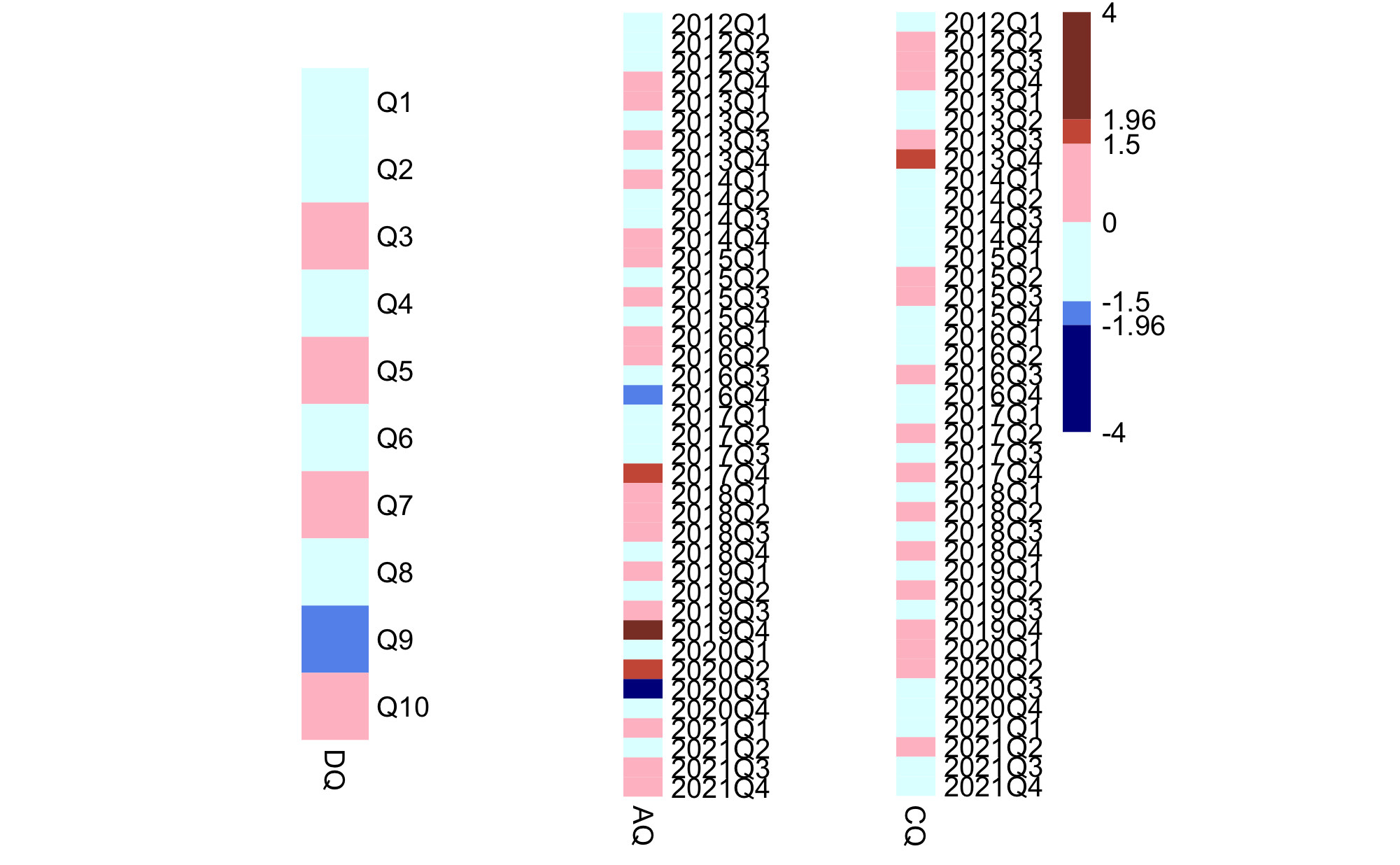
Figure A: Heatmaps of Z score by development quarters, accident quarters, and calendar quarters

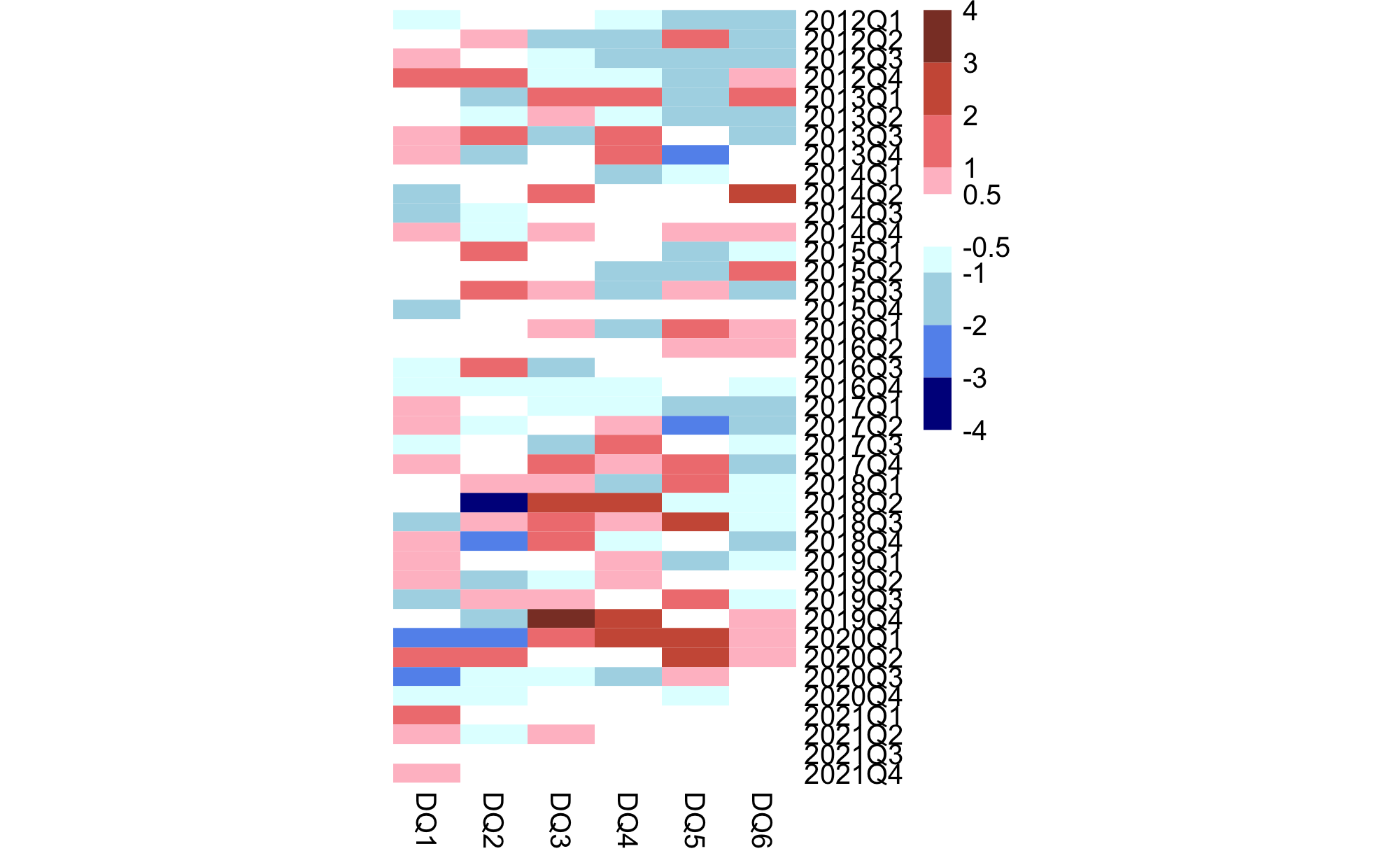
Figure B: Heatmap of deviance residuals

E Frequency trend

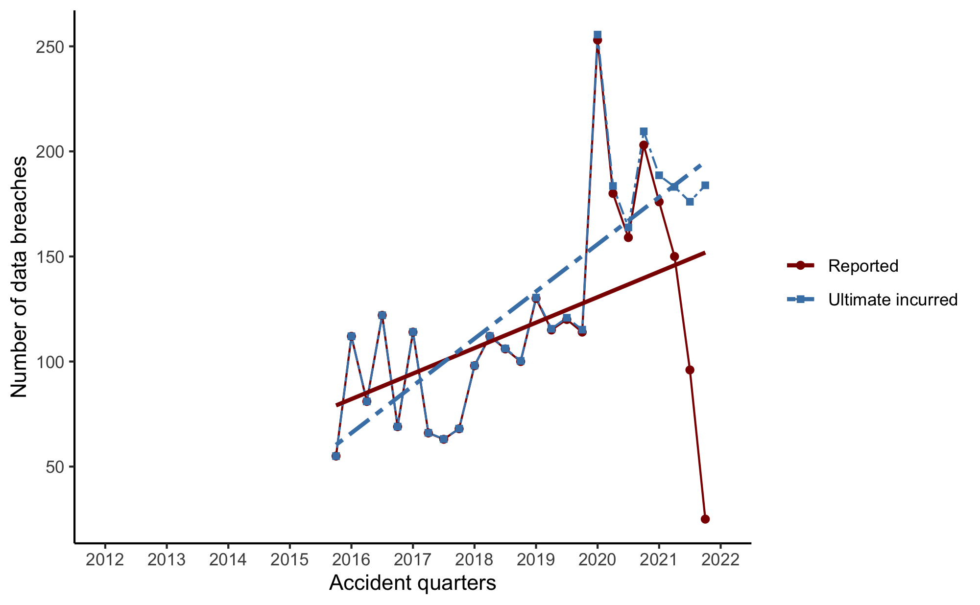
Figure C: Reported versus Ultimate incurred breaches (AQ 2015Q4 - 2021Q4, MT(0-249))

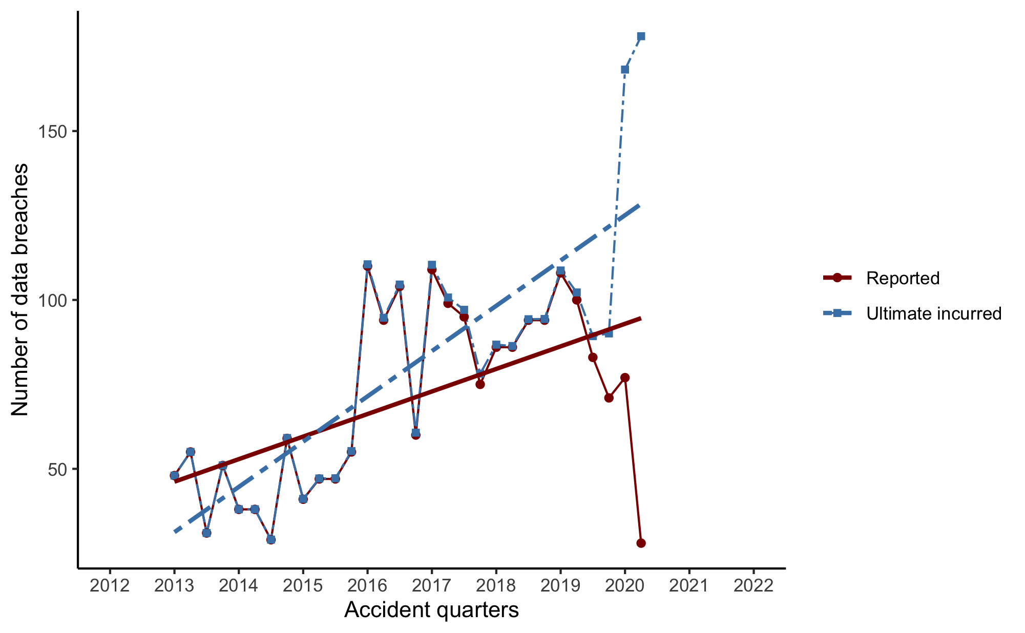
Figure D: Reported versus Ultimate incurred breaches (AQ 2013Q1 - 2020Q2, ME(0-249))

F Interactions between development periods and accident periods

F.1 CA($>$499)

Figures E - G show the trends in development pattern of breaches that affect more than 500 California residents between 2012Q1 and 2021Q4. On average, around 80$\%$ of breaches are disclosed within the first four quarters of occurrence, and 90$\%$ within six quarters. The change in development pattern manifests itself in the first four DQs. Fitted incremental and cumulative percentage of breaches reported in DQ 1-4 are plotted respectively, based on the total number of breaches including IBNRs.

There are two change-points: 2014Q3 and 2017Q1. From 2012Q1 to 2014Q3, the incremental percentage of breaches reported in DQ 1 becomes larger, and smaller in DQ 2-4 respectively. The cumulative percentage of breaches starting from DQ 2 becomes smaller, and the cumulative percentage of breaches reported within one year from occurrence decreases from 86$\%$ to 79$\%$.

From 2014Q3 to 2017Q1, the changes are reversed. The incremental percentage of breaches reported in DQ 1 becomes smaller, and larger in DQ 2-4 respectively. However, while the cumulative percentage in DQ 1 and DQ 2 becomes lower, it becomes larger in DQ 3 and DQ 4. The cumulative percentage of breaches reported within one year from occurrence increases from 79$\%$ to 83$\%$.

Although the period between 2017Q1 and 2021Q4 continues the same pattern of change as the period between 2014Q3 to 2017Q1, that is, the incremental percentage of breaches reported in DQ 1 becomes smaller, and larger in DQ 2-4 respectively, the magnitude of change is greater. The percentage of breaches reported in DQ 1 decreases from 28$\%$ to 12$\%$. The cumulative percentage in all DQs before DQ 4 becomes lower, and finally in DQ 4, catches up to the level observed for breaches occurred in 2017Q1. The cumulative percentage of breaches reported within one year from occurrence keeps around 83$\%$.

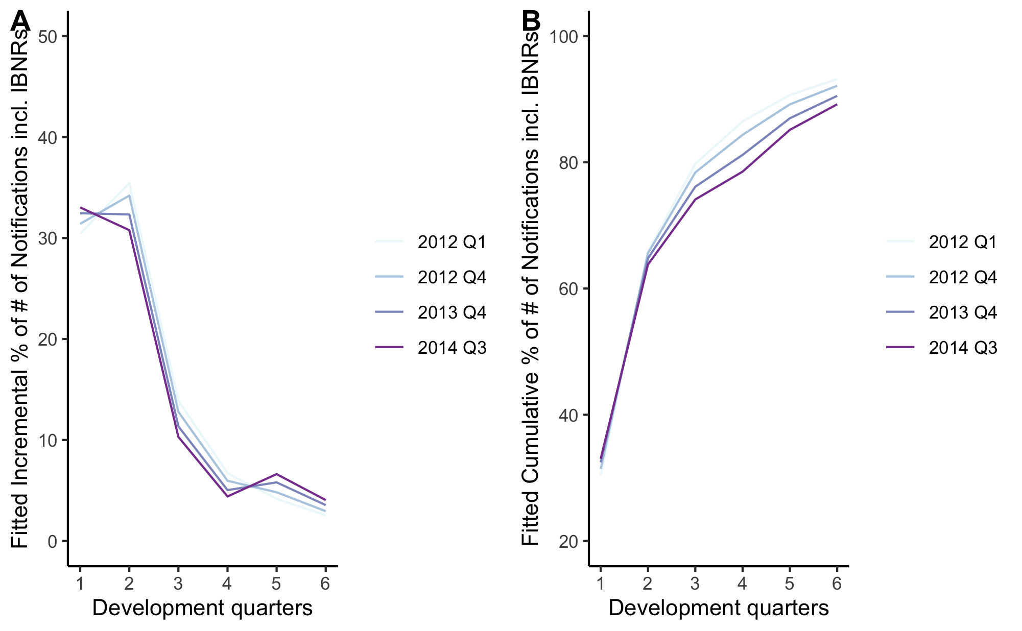
Figure E: Development pattern trend (AQ 2012Q1 - AQ 2014Q3, CA($>$499))

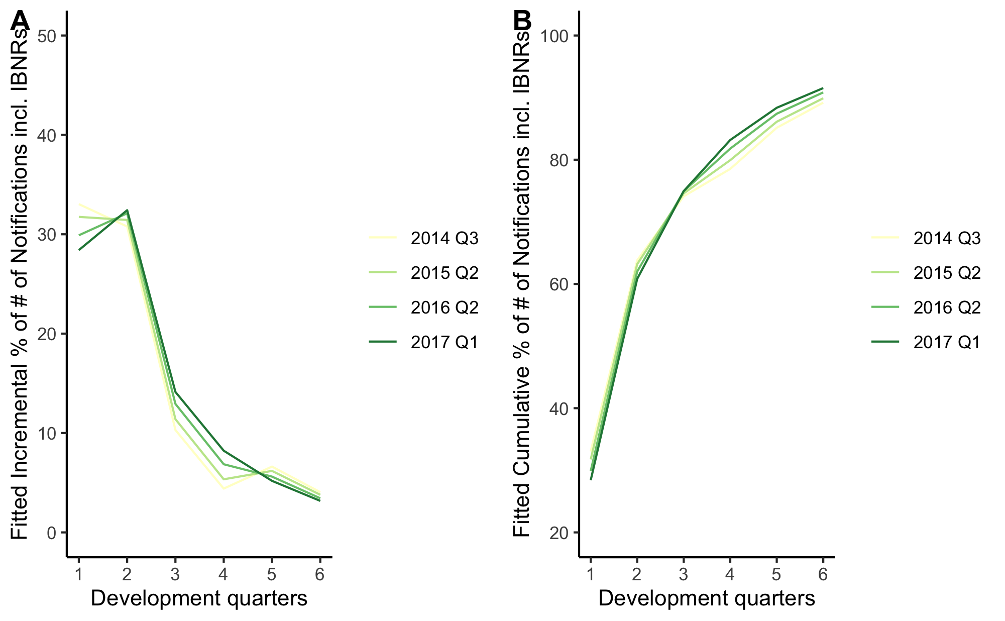
Figure F: Development pattern trend (AQ 2014Q3 - AQ 2017Q1, CA($>$499))

Figure G: Development pattern trend (AQ 2017Q1 - AQ 2021Q4, CA($>$499))

F.2 IN(0-249)

Figure H shows the trend in development pattern of breaches that affect between 0 and 249 Indiana residents between 2014Q1 and 2021Q2. On average, around 90$\%$ of breaches are disclosed within four quarters of occurrence, and almost all breaches are reported within six quarters. The change in development pattern is observed in the first six DQs. Fitted incremental and cumulative percentage of breaches reported in DQ 1-6 are plotted respectively, based on the total number of breaches including IBNRs.

In the period between 2014Q1 and 2017Q3, data breaches are subject to a constant development pattern and 2017Q4 is the point of change. From 2017Q4 onward, the incremental percentage of breaches reported in DQ 1 and DQ 2 becomes smaller, and larger in all subsequent DQs. The cumulative percentage in all DQs before DQ 6 is consistently lower than before, until which it catches up to the level observed for breaches occurred in 2017Q3. Cumulative percentage of breaches reported within one year from occurrence decreases from 93$\%$ to 87$\%$, and cumulative percentage within six quarters increases from 96$\%$ to 98$\%$, when comparing 2017Q3 and 2021Q2.

Figure H: Development pattern trend (AQ 2014Q1 - AQ 2021Q2, IN (0-249))

F.3 MT(0-249)

Figure I shows the trend in development pattern of breaches that affect between 0 and 249 Montana residents between 2015Q4 and 2021Q4. On average, around 90$\%$ of breaches are disclosed within four quarters of occurrence, and almost all breaches are reported within six quarters. The change in development pattern is observed in the first six DQs. Fitted incremental and cumulative percentage of breaches reported in DQ 1-6 are plotted respectively, based on the total number of breaches including IBNRs.

In the period between 2015Q4 and 2017Q3, data breaches are subject to a constant development pattern and 2017Q4 is the point of change. From 2017Q4 onward, the incremental percentage of breaches reported in DQ 1 becomes smaller, larger in all DQs between DQ 2 and DQ 4, and smaller in DQ 5 and DQ 6. The cumulative percentage is lower in the first two DQs, but higher in all later DQs. Cumulative percentage of breaches reported within one year from occurrence increases from 86$\%$ to 94$\%$, and cumulative percentage within six quarters increases from 92$\%$ to 98$\%$, when comparing 2015Q4 and 2021Q2.

Figure I: Development pattern trend (AQ 2015Q4 - AQ 2021Q4, MT (0-249))

F.4 ME(0-249)

Figures J and K show the trends in development pattern of breaches that affect between 0 and 249 Maine residents between 2013Q1 and 2020Q2. On average, around 90$\%$ of breaches are disclosed within four quarters of occurrence, and almost all breaches are reported within six quarters. The change in development pattern is observed in the first six DQs. Fitted incremental and cumulative percentage of breaches reported in DQ 1-6 are plotted respectively, based on the total number of breaches including IBNRs.

In the period between 2013Q1 and 2017Q3, data breaches are subject to a constant development pattern. Data breaches occurred in 2017Q4 are more delayed: the cumulative percentage at all DQs is lower. Then, between 2018Q1 and 2018Q4, the delay is shortening. The cumulative percentage at DQ 1 and DQ 2 is indistinguishable from that of breaches occurred in 2018Q1, but the cumulative percentage at all subsequent DQs is higher.

From 2018Q4 onward, the incremental percentage of breaches reported in DQ 1 and DQ 2 becomes smaller, larger in DQ 3 and DQ 4, and smaller in DQ 5 and DQ 6. The cumulative percentage is lower in the first two DQs, but higher in all later DQs. Cumulative percentage of breaches reported within one year from occurrence increases from 90$\%$ to 94$\%$, and cumulative percentage within six quarters increases from 94$\%$ to 100$\%$, when comparing 2013Q1 and 2020Q2.

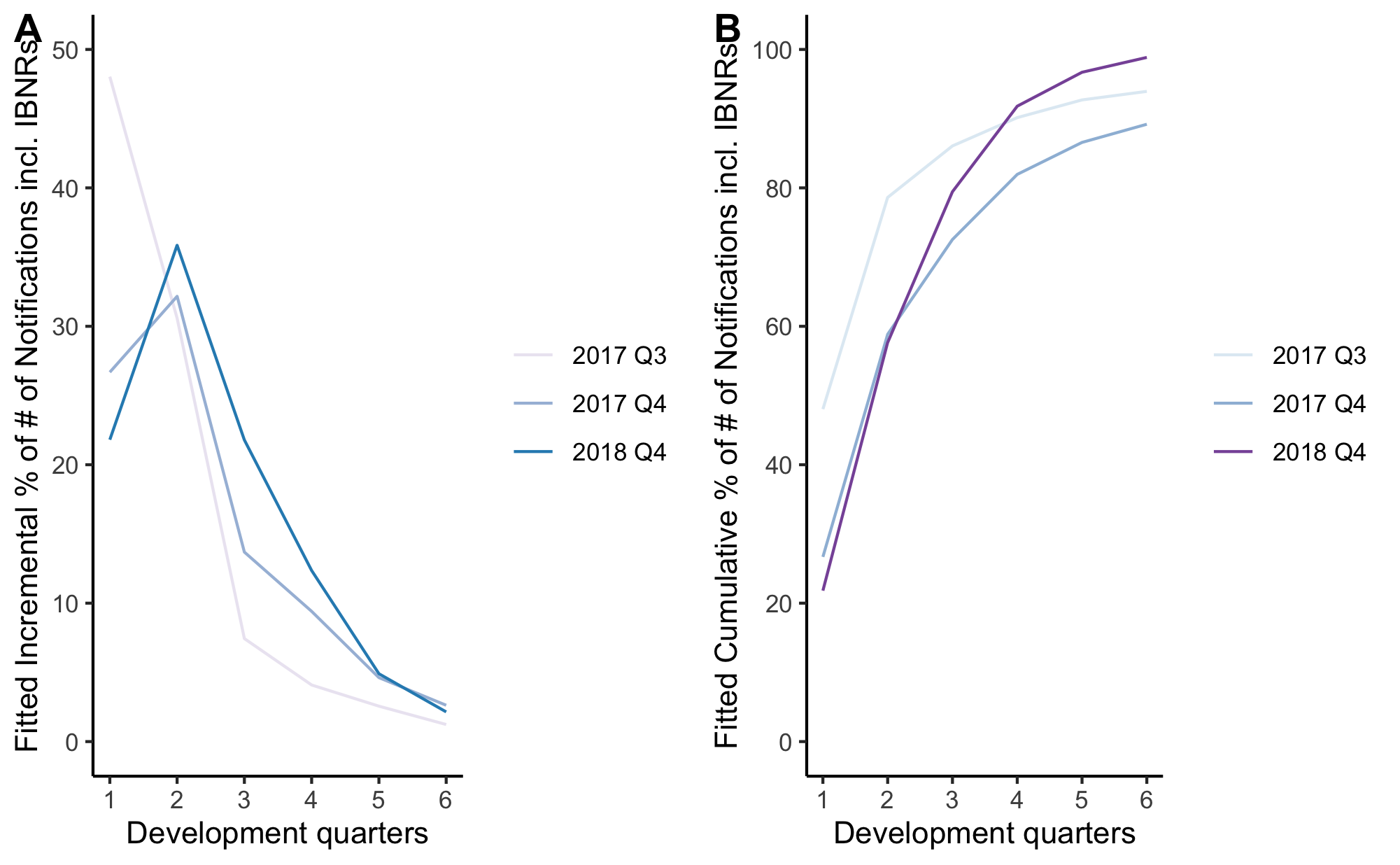
Figure J: Development pattern trend (AQ 2013Q1 - AQ 2018Q4, ME (0-249))

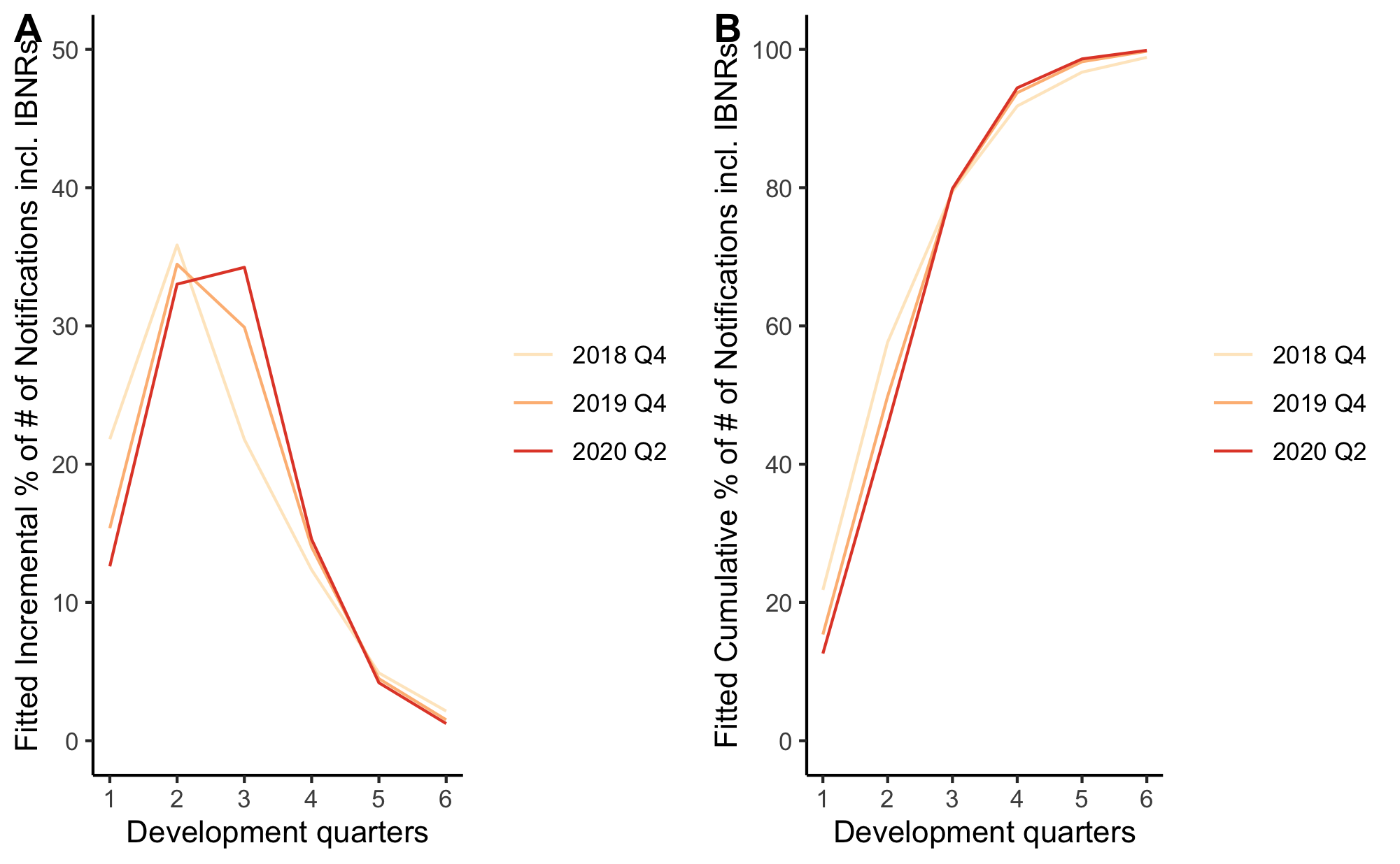
Figure K: Development pattern trend (AQ 2018Q4 - AQ 2020Q2, ME (0-249))

G Average reporting delay

G.1 MT(0-249)

Shown in Figure L, the average time to report data breaches is 2.64 quarters between 2013Q1 and 2017Q3, increases to 2.68 quarters in 2017Q4, and gradually decreases to the same level as before. The average reporting delay is fairly constant over time.

Figure L: Fitted average delay and its trend - MT(0-249)

G.2 ME(0-249)

Shown in Figure M, the average time to report data breaches is 2.39 quarters between 2015Q4 and 2017Q3, increases to 2.7 quarters in 2018Q1, decreases at a decreasing rate until 2018Q4 to 2.54 quarters, and increases slightly to 2.69 quarters in 2020Q2.

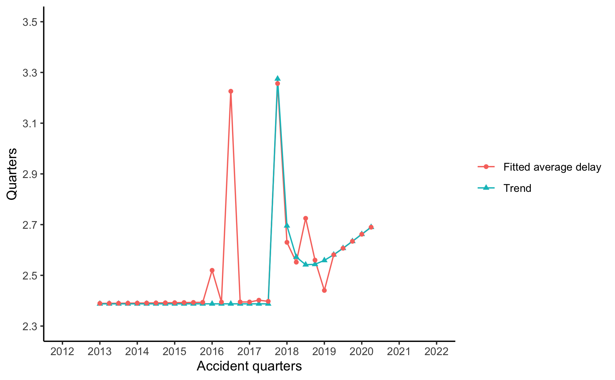
Figure M: Fitted average delay and its trend - ME(0-249)

References

- Allianz (2022) Allianz, 2022. Allianz risk barometer 2022: Cyber perils outrank covid-19 and broken supply chains as top global business risk. URL: https://www.allianz.com/en/press/news/studies/220118_Allianz-Risk-Barometer-2022.html. last accessed: Jun 23, 2023.
- Allianz (2023) Allianz, 2023. Allianz risk barometer 2023. URL: https://www.agcs.allianz.com/news-and-insights/reports/allianz-risk-barometer.html#download. last accessed: Jun 23, 2023.
- Antonio and Beirlant (2008) Antonio, K., Beirlant, J., 2008. Issues in claims reserving and credibility: a semiparametric approach with mixed models. Journal of Risk and Insurance 75, 643–676.
- Aon (2021) Aon, 2021. 2021 global risk management survey. URL: https://grms.aon.com/2021-global-risk-management-survey/. last accessed: Jun 23, 2023.
- Attorney General of Texas (2023) Attorney General of Texas, 2023. Data security breach reports. URL: https://oag.my.site.com/datasecuritybreachreport/apex/DataSecurityReportsPage. last accessed: Jun 23, 2023.
- Benaroch (2021) Benaroch, M., 2021. Third-party induced cyber incidents—much ado about nothing? Journal of Cybersecurity 7, tyab020.
- Bessy-Roland et al. (2021) Bessy-Roland, Y., Boumezoued, A., Hillairet, C., 2021. Multivariate hawkes process for cyber insurance. Annals of Actuarial Science 15, 14–39.