Two-stage Crash Process in Resistive Drift Ballooning Mode Driven ELM Crash

Abstract

We report a two-stage crash process in edge localized mode (ELM) driven by resistive drift-ballooning modes (RDBMs) numerically simulated in a full annular torus domain. In the early nonlinear phase, the first crash is triggered by linearly unstable RDBMs and $m/n=2/1$ magnetic islands are nonlinearly excited via nonlinear couplings of RDBMs. Simultaneously, middle-$n$ RDBM turbulence develops but is poloidally localized around X-points of the magnetic islands, leading to the small energy loss. Here $m$ is the poloidal mode number, $n$ is the toroidal mode number, the $q=2$ rational surface exists at the pressure gradient peak, and $q$ is the safety factor, respectively. The second crash occurs in the late nonlinear phase. Low-$n$ magnetic islands are also excited around the $q=2$ surface via nonlinear couplings among the middle-$n$ turbulence. Since the turbulence develops from the X-points of higher harmonics of $m/n=2/1$ magnetic islands, it expands out poloidally. The second crash is triggered when the turbulence covers the whole poloidal region. A scan of toroidal wedge number $N$, where full torus is divided into $N$ segments in the toroidal direction, also reveals that the first crash process becomes more prominent with the higher toroidal wedge number where the RDBMs play a dominant role. These results indicate that nonlinear interactions of all channels in the full torus domain can significantly affect the trigger dynamics of ELMs driven by the RDBMs.

I Introduction

The intermittent heat loads by edge localized modes (ELMs) Zohm (1996) in H-mode tokamak plasma Wagner et al. (1982) should be avoided or mitigated below heat load constraints on plasma facing components, which is one of key issues for ITER Kukushkin et al. (2011); Gunn et al. (2017) and DEMO Asakura et al. (2021). Nonlinear numerical simulations are powerful tools to understand ELM dynamics and to calculate ELM energy loss so that several nonlinear MHD codes such as JOREK Huysmans and Czarny (2007); Czarny and Huysmans (2008); Hoelzl et al. (2021), NIMROD Sovinec et al. (2004), M3D-C1 Ferraro, Jardin, and Snyder (2010); Wingen et al. (2015), MEGA Todo and Sato (1998); Todo et al. (2017); Rivero Rodriguez et al. (2023) and BOUT++ Dudson et al. (2009); Xu et al. (2010); Zhu et al. (2021) have been developed and have provided qualitative understanding of ELMs.

BOUT++ code is a plasma fluid simulation framework solving plasma fluid equations as initial value problems in arbitrary curvilinear coordinate systems with finite difference methods. For three dimensional tokamak boundary plasma simulations including ELMs, BOUT++ code employs the quasi-ballooning coordinate system Dudson et al. (2009) consisting of orthogonal flux surface coordinates D’haeseleer et al. (1991) for differences in the radial direction and field aligned coordinates Beer, Cowley, and Hammett (1995) for differences along the equilibrium magnetic field line. With this coordinate system, BOUT++ code can calculate middle-$n$ $(\mathcal{O}(n)>1)$ and high-$n$ $(\mathcal{O}(n)\gg 1)$ plasma instabilities with reasonable computational cost and high accuracy, which is suitable for simulations of ELMs by the ballooning modes.

Its computation domain was however limited to an $1/N$-th annular toroidal wedge to remove low-$n$ $(\mathcal{O}(n)\sim 1)$ mode components from the system to avoid numerical instabilities. Here, in the $1/N$-th annular toroidal wedge torus, a full torus domain is divided equally into $N$ parts in the toroidal direction. This is because the flute-ordering approximation neglecting differences along the magnetic field is required in the field solver of flow potential in the quasi-ballooning coordinate system.

Recently we have resolved this issue by implementing a hybrid field solver Seto et al. (2023) consisting of a 2D field solver for $n=0$ and low-$n$ modes, and a flute-ordered 1D field solver for moderate-$n$ and high-$n$ modes to address ELM crash simulations in the full annular torus domain. Taking the full annular torus domain is important not only for simulating ELMs by kink/peeling modes, ELMs with resonant magnetic perturbations (RMPs) Evans et al. (2004); Orain et al. (2013), QH-mode accompanied with low-$n$ edge harmonic oscillations Burrell et al. (2002); Liu et al. (2015) but also for simulating ELMs by ballooning modes, ELMs with turbulence transport and so on. For example, the number of nonlinear mode-mode couplings in the simulated system can change the nonlinear criterion of the ELM crash Xi, Xu, and Diamond (2014). A full-f core gyrokinetic simulation reveals that using too large toroidal wedge number $N$ can result in the false convergence of turbulence heat transport level Kim et al. (2017), which may also occur in edge turbulence transport simulations.

Our recent work Seto et al. (2023) also shows that taking full annular torus domain can qualitatively change crash process of the ELMs by the resistive drift ballooning modes (RDBMs) compared to that in a quarter torus domain with $N=4$, however the crash mechanism has not been clarified in detail. In this paper, the RDBM-driven ELM in the full annular torus domain is analyzed to understand its crash mechanism as well as quantitative difference between ELMs with different toroidal wedge numbers.

The rest of this paper is organized as followings. A set of governing equation and a MHD equilibrium used for ELM crash simulations are described in Sec.II. The crash process in the ELM crash in the full annular torus domain is analyzed. The crash mechanism is discussed in detail. In addition, the impact of the wedge torus domain on ELM crash is also discussed in Sec.III. The paper is finally summarized in Sec. IV.

II Simulation setup

The following scale-separated four-field reduced model with the flat ion density profile $n_{\rm i}=\bar{n_{\rm i}}$ describing the RDBM Seto et al. (2020) is employed for ELM crash simulations,

$$\frac{\partial{\varpi}_{1}}{\partial t} = -\left[{F}_{1},\varpi\right]-\left[{F}_{0},{\varpi}_{1}\right]+\mathcal{G}\left({P}_{1},F\right)+\mathcal{G}\left({P}_{0},{F}_{1}\right)$$ (1)

$$+\mathcal{K}\left({P}_{1}\right)-{B}_{0}\partial_{\parallel}\left(\frac{{J_{\parallel}}_{1}}{{B}_{0}}\right)+{B}_{0}\left[{A_{\parallel}}_{1},\frac{J_{\parallel}}{{B}_{0}}\right]+\mu_{\parallel}\partial_{\parallel}^{2}{\varpi}_{1}+\mu_{\perp}\nabla^{2}_{\perp}{\varpi}_{1},$$

$$\frac{\partial{A_{\parallel}}_{1}}{\partial t} = -\left[\phi,{A_{\parallel}}_{1}\right]-\partial_{\parallel}{\phi}_{1}+\delta\left(\partial_{\parallel}{P}_{1}-\left[{A_{\parallel}}_{1},P\right]\right)+\eta{J}_{1}-\lambda\nabla_{\perp}^{2}{J}_{1},$$ (2)

$$\frac{\partial{P}_{1}}{\partial t} = -\left[\phi_{1},P\right]-\left[\phi_{0},P_{1}\right]-2\beta_{*}\mathcal{K}\left({\phi}_{1}\right)$$ (3)

$$-\beta_{*}{B}_{0}\partial_{\parallel}\left(\frac{{v}_{1}+d_{\mathrm{i}}{J_{\parallel}}_{1}}{{B}_{0}}\right)+\beta_{*}{B}_{0}\left[{A_{\parallel}}_{1},\frac{{v}_{1}+d_{\mathrm{i}}{J_{\parallel}}_{1}}{{B}_{0}}\right]+\chi_{\parallel}\partial_{\parallel}^{2}{P}_{1}+\chi_{\perp}\nabla_{\perp}^{2}{P}_{1},$$

$$\frac{\partial{v_{\parallel}}_{1}}{\partial t} = -\left[\phi,{v_{\parallel}}_{1}\right]-\frac{1}{2}\partial_{\parallel}{P}_{1}+\frac{1}{2}\left[{A_{\parallel}}_{1},P\right]+\nu_{\perp}\nabla_{\perp}^{2}{v_{\parallel}}_{1},$$ (4)

$$\varpi = \nabla_{\perp*}^{2}F,\quad{\phi}_{0}=-\delta{P}_{0},\quad\quad{J_{\parallel}}_{1}=\nabla_{\perp}^{2}{A_{\parallel}}_{1},\quad{\bm{B}}_{1}=\nabla{A_{\parallel}}_{1}\times{\bm{b}}_{0}$$

$$\partial_{\parallel}f = {\bm{b}}_{0}\cdot\nabla f,\quad\partial_{\parallel}^{2}f=\partial_{\parallel}\left(\partial_{\parallel}f\right),\quad\nabla_{\perp}f=\nabla f-{\bm{b}}_{0}{\bm{b}}_{0}\cdot\nabla f,\quad\nabla_{\perp}^{2}f=\nabla\cdot\nabla_{\perp}f,$$

$$\left[f,g\right] = \frac{{\bm{b}}_{0}\times\nabla_{\perp}f\cdot\nabla_{\perp}g}{{B}_{0}},\quad\nabla_{\perp*}^{2}f=\nabla\cdot\left(\frac{\nabla_{\perp}f}{{B}_{0}^{2}}\right),\quad\mathcal{K}\left(f\right)=\frac{{\bm{b}}_{0}\times{\bm{\kappa}}_{0}\cdot\nabla f}{{B}_{0}},$$

$$\mathcal{G}\left(f,g\right) = \frac{\delta}{2}\left(\left[f,\nabla_{\perp*}^{2}g\right]+\left[f,\nabla_{\perp*}^{2}g\right]+\nabla_{\perp*}^{2}\left[f,g\right]\right).$$

Here $\varpi$ is the vorticity defined with the generalized flow potential $F=\phi+\delta P$, $P={P}_{0}+{P}_{1}$ is the plasma pressure, $\phi={\phi}_{0}+{\phi}_{1}$ is the electrostatic potential, $\delta=d_{\rm i}/4$ is the factor for electron and ion diamagnetism for the isotropic pressure case $P_{\rm e}=P_{\rm i}=P/2$, $d_{\rm i}$ is the ion skin depth, $J_{\parallel}={J_{\parallel}}_{0}+{J_{\parallel}}_{1}$ is the parallel current density, $A_{\parallel}={A_{\parallel}}_{1}$ is the parallel magnetic potential, $\bm{B}={\bm{B}}_{0}+{\bm{B}}_{1}$ is the magnetic field intensity, $\mu_{\parallel}$ is the parallel viscosity for vorticity $\mu_{\perp}$ is the perpendicular viscosity for vorticity, $\eta$ is the resistivity, $\lambda$ is the hyper-resistivity, $\beta_{*}={B}_{0}^{2}/[0.5+{B}_{0}^{2}/(5{P}_{0}/3)]$ is the compression factor, ${\bm{b}}_{0}={\bm{B}}_{0}/{{B}_{0}}$ is the unit vector along the equilibrium magnetic field, ${\bm{\kappa}}_{0}={\bm{b}}_{0}\cdot\nabla{\bm{b}}_{0}$ is the magnetic curvature, $v_{\parallel}$ is the ion parallel flow, $\chi_{\parallel}$ is the parallel heat diffusivity, $\chi_{\perp}$ is the perpendicular heat diffusivity, and $\nu_{\perp}$ is the perpendicular viscosity for parallel flow, respectively. In this model, the subscript “0” represents an equilibrium part and the subscript “1” represents a perturbed part of physical quantities, $f(\bm{x},t)={f}_{0}(\bm{x})+{f}_{1}(\bm{x},t)$. The ion gyroviscous cancellation is modeled in the Chang-Callen manner Chang and Callen (1992) in the vorticity equation and the set of equations is normalized with poloidal Alfvén unit with the reference length $\bar{R}=3.5~{}[\mathrm{m}]$, the reference magnetic intensity $\bar{B}=2.0~{}[\mathrm{T}]$, the reference ion number density $\bar{n_{\rm i}}=1.0\times 10^{19}~{}[\mathrm{m}^{-3}]$, the deuterium mass and the effective charge number $Z=1.0$.

In this paper, we employ constant resistivities $\eta=1.0\times 10^{-8}$ and $\lambda=1.0\times 10^{-12}$, and viscosities and diffusivities$\mu_{\perp}=\chi_{\perp}=\nu_{\perp}=1.0\times 10^{-7}$ and $\mu_{\parallel}=\chi_{\parallel}=1.0\times 10^{-1}$ as our previous works Seto et al. (2023, 2020). It should be noted that the equilibrium $E\times B$ flow, or the equilibrium radial electric field, is modeled to cancel with the equilibrium ion diamagnetic flow ${F}_{0}=0$ so that the neoclassical poloidal flow and its return flow Itoh and Itoh (1996) are not taken into account. Modeling the return flow is a key to simulate the bifurcation between zonal flow and streamer formation, which is left for future works. It should be also noted that the anomalous electron heat diffusivity Rechester and Rosenbluth (1978) and the hyper-resistivity by magnetic stochastisation Kaw, Valeo, and Rutherford (1979) are not taken into account due to the usage of the constant hyper-resistivity and the linearized second parallel derivative $\partial_{\parallel}^{2}$ lacking magnetic flatter effects. This means that ELM energy loss in this work is driven by $E\times B$ convection and numerical diffusion. These are left for future works.

The computational grid for the orthogonal flux surface coordinate system $(\psi,\theta,\zeta)$ and plasma profiles used in the ELM crash simulations are shown in Fig. 1. Here the $\psi$ is the poloidal flux function, $\theta$ is the orthogonal poloidal angle and $\zeta$ is the geometrical toroidal angle, respectively. The computational grid is constructed from a shifted circular equilibrium marginally unstable against ideal ballooning mode Wilson et al. (2002); Snyder et al. (2002) generated by TOQ equilibrium code Miller and Vandam (1987); Burke et al. (2010). The quasi-ballooning coordinate system Dudson et al. (2009) consists of the flux surface coordinate system $(\psi,\theta,\zeta)$ and the field-aligned coordinate system $(x,y,z)$, where $x=\psi$ is the radial label, $y=\theta$ is the parallel label, and $z=\zeta-\alpha$ is the binormal label with the shift angle $\alpha=\int_{\pi}^{\theta}({\bm{B}}_{0}\cdot\nabla\zeta/{\bm{B}}_{0}\cdot\nabla\theta)d\theta$, respectively. The coordinate transform between the flux surface coordinate system and the field-aligned coordinate system is performed in the Fourier space with respect to the toroidal mode number $n$ using the phase relation $z=\zeta-\alpha$, which is briefly reviewed in Ref. Seto et al. (2019).

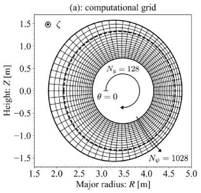
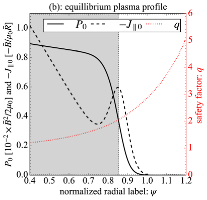
Figure 1: (a): computational grid based on the shifted circular equilibrium and (b): its plasma profiles; the equilibrium plasma pressure ${P}_{0}$ (black solid), the equilibrium parallel current density ${J_{\parallel}}_{0}$ on the outer mid-plane (black dashed) and the safety factor $q$ (red dotted), respectively.

The linear growth rate of RDBMs for this equilibrium is shown in Fig. 2. The largest growth rate is given by $\gamma/\omega_{A}=7.86\times 10^{-2}$ for the toroidal mode number $n=32$. It is found that the RDBMs are stable for $n\leq 10$ and $n\geq 53$.

For ELM crash simulations, the number of radial grids $N_{\psi}$ is 1028 for $0.4\leq\psi\leq 1.2$ and the number of parallel grids (or poloidal grids) $N_{y}$ is 128. The number of binormal grids (or toroidal grids) $N_{z}$ is $256/N$ for $0\leq z<2\pi/N$, where the grid width in the binormal direction is kept constant for different toroidal wedge numbers. Here the radial and poloidal grid resolutions are fine enough, which is discussed in section 5.2 in Ref. Seto et al. (2023). In the hybrid field solver calculating the generalized flow potential Seto et al. (2023), $0\leq n\leq 4$ mode components are calculated by the 2D field solver and $4<n\leq 80$ mode components are calculated by the flute-ordered 1D field solver, where $n\geq 81$ components are removed with a low-pass filter. In all ELM crash simulations reported in this work, initial perturbations are set on all modes except $n=0$ mode to introduce nonlinear couplings Xi, Xu, and Diamond (2014) self-consistently. The set of radial boundary conditions is the Neumann boundary condition $\partial_{\psi}f=0$ at the inner boundary $\psi=0.4$ and Dirichlet boundary condition $f=0$ at the outer boundary $\psi=1.2$ for $f={\varpi}_{1},{P}_{1},{A_{\parallel}}_{1},{v_{\parallel}}_{1},{F}_{1},{J_{\parallel}}_{1}$.

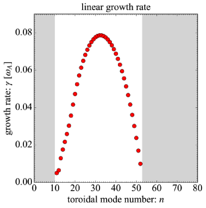
Figure 2: linear growth rate of RDBM instability, where the shaded regions $0\leq n\leq 10$ and $n\geq 53$ are stable against RDBM instability.

III Two-stage crash process in RDBM-driven ELM crash

In the first part of this section, the crash process in the RDBM-driven ELM crash in the full annular torus domain with $N=1$ Seto et al. (2023) is analyzed in detail. In the second part of this section, the dependence of toroidal wedge numbers with $N=1,2,4$ on the ELM crash process is investigated to understand the qualitative difference of them.

The time evolution of the ELM energy loss level and its change rate in the full torus case are summarized in Fig. 3, where the time label is set to be $t=0t_{A}$ at the time when the $n=32$ component of the perpendicular kinetic energy gets saturated. Here, the energy loss level $\Delta W_{\rm ped}/W_{\rm ped}$ is defined by the ratio of the energy lost from the region inside the rational surface of the initial pressure gradient peak $V_{\rm ped}$ highlighted with the black dotted line and shaded area in Fig. 1(b),

$$\Delta W_{\rm ped}/W_{\rm ped}=-\int_{V_{\rm ped}}{P}_{1}dV/\int_{V_{\rm ped}}{P}_{0}dV.$$ (5)

It is clear that the change rate of the energy loss level has the two peaks at $t=0t_{A}$ and $t=103t_{A}$. Hereafter we define the first peak at $t=0t_{A}$ to be the first crash and the second peak at $t=103t_{A}$ as the second crash, respectively.

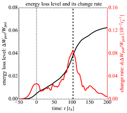
Figure 3: time evolution of ELM energy loss level $\Delta W_{\rm ped}/W_{\rm ped}$ with the black solid curve and the left vertical axis and that of change rate of ELM energy loss level $\partial_{t}\Delta W_{\rm ped}/W_{\rm ped}$ with the red solid curve and the right vertical axis in the full torus case. Here the first crash at $t=0t_{A}$ is highlighted with the black dotted line and the second crash at $t=103t_{A}$ is highlighted with the black dashed line, respectively.

Equations of the system energies in this model are defined as the followings. The equation of $n=n^{\prime}$ component of volume-averaged perpendicular kinetic energy $W_{\rm k}(t,n^{\prime})$ can be derived from vorticity equation Eq. (1) by multiplying with $n=n^{\prime}$ component of the generalized flow potential ${F}_{1}^{n=n^{\prime}}$ and taking its volume average over the computation domain $V$,

$$\frac{\partial}{\partial t}W_{\rm k}(t,n^{\prime}) = T_{\rm k,RS}^{\rm nl}(t,n^{\prime})+T_{\rm k,CV}^{\rm li}(t,n^{\prime})+T_{\rm k,LB}^{\rm li}(t,n^{\prime})+T_{\rm k,MS}^{\rm nl}(t,n^{\prime})+T_{\rm k,VD}^{\rm li}(t,n^{\prime}),$$ (6)

with

$$W_{\rm k}(t,n^{\prime}) = \langle\frac{1}{2{B}_{0}^{2}}\left|\nabla_{\perp}{F}_{1}^{n=n^{\prime}}\right|^{2}\rangle_{V},$$ (7)

and

$$T_{\rm k,RS}^{\rm nl}(t,n^{\prime}) = \langle{F}_{1}^{n=n^{\prime}}\left[{F}_{1},\varpi\right]\rangle_{V}+\langle{F}_{1}^{n=n^{\prime}}\left[{F}_{0},{\varpi}_{1}\right]\rangle_{V}-\langle{F}_{1}^{n=n^{\prime}}\mathcal{G}\left({P}_{1},F\right)\rangle_{V}-\langle{F}_{1}^{n=n^{\prime}}\mathcal{G}\left({P}_{0},{F}_{1}\right)\rangle_{V},$$ (8)

$$T_{\rm k,CV}^{\rm li}(t,n^{\prime}) = -\langle{F}_{1}^{n=n^{\prime}}\mathcal{K}\left({P}_{1}\right)\rangle_{V},$$ (9)

$$T_{\rm k,LB}^{\rm li}(t,n^{\prime}) = \langle{F}_{1}^{n=n^{\prime}}{B}_{0}\partial_{\parallel}\left(\frac{{J_{\parallel}}_{1}}{{B}_{0}}\right)\rangle_{V},$$ (10)

$$T_{\rm k,MS}^{\rm nl}(t,n^{\prime}) = -\langle{F}_{1}^{n=n^{\prime}}{B}_{0}\left[{A_{\parallel}}_{1},\frac{J_{\parallel}}{{B}_{0}}\right]\rangle_{V},$$ (11)

$$T_{\rm k,VD}^{\rm li}(t,n^{\prime}) = -\langle{F}_{1}^{n=n^{\prime}}\mu_{\parallel}\partial_{\parallel}^{2}{\varpi}_{1}\rangle_{V}-\langle{F}_{1}^{n=n^{\prime}}\mu_{\perp}\nabla^{2}_{\perp}{\varpi}_{1}\rangle_{V},$$ (12)

where $T_{\rm k,RS}^{\rm nl}(t,n^{\prime})$ is the contribution from Reynolds stress terms, $T_{\rm k,CV}^{\rm li}(t,n^{\prime})$ is the contribution from geodesic curvature term, $T_{\rm k,LB}^{\rm li}(t,n^{\prime})$ is the contribution from line-bending term, $T_{\rm k,MS}^{\rm nl}(t,n^{\prime})$ is the contribution from Maxwell stress term, $T_{\rm k,VD}^{\rm li}(t,n^{\prime})$ is the energy loss by numerical viscosity terms, and $\langle f\rangle_{V}=V^{-1}\int_{V}fdV$ is the volume average operation, respectively. The equation of $n=n^{\prime}$ component of volume-averaged magnetic energy $W_{\rm m}(t,n^{\prime})$ can be also derived from Ohm’s law Eq. (2) as,

$$\frac{\partial}{\partial t}W_{\rm m}(t,n^{\prime}) = T_{\rm m,EH}^{\rm li}(t,n^{\prime})+T_{\rm m,EH}^{\rm nl}(t,n^{\prime})+T_{\rm m,RD}^{\rm li}(t,n^{\prime}),$$ (13)

with

$$W_{\rm m}(t,n^{\prime}) = \langle\frac{1}{2}\left|\nabla_{\perp}{A_{\parallel}}_{1}^{n=n^{\prime}}\right|^{2}\rangle_{V},$$ (14)

and

$$T_{\rm m,EH}^{\rm li}(t,n^{\prime}) = \langle{J_{\parallel}}_{1}^{n=n^{\prime}}\partial_{\parallel}\left({\phi}_{1}-\delta{P}_{1}\right)\rangle_{V},$$ (15)

$$T_{\rm m,EH}^{\rm nl}(t,n^{\prime}) = -\langle{J_{\parallel}}_{1}^{n=n^{\prime}}\left[{A_{\parallel}}_{1},\phi-\delta P\right]\rangle_{V},$$ (16)

$$T_{\rm m,RD}^{\rm li}(t,n^{\prime}) = -\langle{J_{\parallel}}_{1}^{n=n^{\prime}}\eta{J_{\parallel}}_{1}\rangle_{V}-\langle\lambda\left|\nabla_{\perp}{J_{\parallel}}_{1}^{n=n^{\prime}}\right|^{2}\rangle_{V},$$ (17)

where $T_{\rm m,EH}^{\rm li}(t,n^{\prime})$ and $T_{\rm m,EH}^{\rm nl}(t,n^{\prime})$ are the linear and nonlinear contribution from electrostatic potential and electron Hall terms, $T_{\rm m,RD}^{\rm li}(t,n^{\prime})$ is the energy loss by the resistive dissipation, respectively. The equation of $n=n^{\prime}$ component of internal energy $W_{\rm p}(t,n^{\prime})$ can be also derived from equation of pressure Eq. (3),

$$\frac{\partial}{\partial t}W_{\rm p}(t,n^{\prime}) = T_{\rm p,PV}^{\rm nl}(t,n^{\prime})+T_{\rm p,CO}(t,n^{\prime})+T_{\rm p,PD}^{\rm li}(t,n^{\prime}),$$ (18)

with

$$W_{\rm p}(t,n^{\prime}) = \langle\frac{1}{4\beta_{*}}\left|{P}_{1}^{n=n^{\prime}}\right|^{2}\rangle_{V},$$ (19)

and

$$T_{\rm p,PV}^{\rm nl}(t,n^{\prime}) = -\langle\frac{1}{2\beta_{*}}{P}_{1}^{n=n^{\prime}}\left[\phi_{1},P\right]\rangle_{V}-\langle\frac{1}{2\beta_{*}}{P}_{1}^{n=n^{\prime}}\left[\phi_{0},P_{1}\right]\rangle_{V},,$$ (20)

$$T_{\rm p,CO}(t,n^{\prime}) = T_{\rm p,CE}^{\rm li}(t,n^{\prime})+T_{\rm p,CJ}^{\rm li}(t,n^{\prime})+T_{\rm p,CJ}^{\rm nl}(t,n^{\prime})+T_{\rm p,CV}^{\rm li}(t,n^{\prime})+T_{\rm p,CV}^{\rm nl}(t,n^{\prime}),$$ (21)

$$T_{\rm p,CE}^{\rm li}(t,n^{\prime}) = -\langle{P}_{1}^{n=n^{\prime}}\mathcal{K}\left({\phi}_{1}\right)\rangle_{V},$$ (22)

$$T_{\rm p,CJ}^{\rm li}(t,n^{\prime}) = -2\delta\langle{P}_{1}^{n=n^{\prime}}{B}_{0}\partial_{\parallel}\left(\frac{{J_{\parallel}}_{1}}{{B}_{0}}\right)\rangle_{V},$$ (23)

$$T_{\rm p,CJ}^{\rm nl}(t,n^{\prime}) = 2\delta\langle{P}_{1}^{n=n^{\prime}}{B}_{0}\left[{A_{\parallel}}_{1},\frac{{J_{\parallel}}_{1}}{{B}_{0}}\right]\rangle_{V},$$ (24)

$$T_{\rm p,CV}^{\rm li}(t,n^{\prime}) = -\frac{1}{2}\langle{P}_{1}^{n=n^{\prime}}{B}_{0}\partial_{\parallel}\left(\frac{{v}_{1}}{{B}_{0}}\right)\rangle_{V},$$ (25)

$$T_{\rm p,CV}^{\rm nl}(t,n^{\prime}) = \frac{1}{2}\langle{P}_{1}^{n=n^{\prime}}{B}_{0}\left[{A_{\parallel}}_{1},\frac{{v}_{1}}{{B}_{0}}\right]\rangle_{V},$$ (26)

$$T_{\rm p,HD}^{\rm li}(t,n^{\prime}) = \langle\frac{{P}_{1}^{n=n^{\prime}}}{2\beta_{*}}\chi_{\parallel}\partial_{\parallel}^{2}{P}_{1}\rangle_{V}+\langle\frac{{P}_{1}^{n=n^{\prime}}}{2\beta_{*}}\chi_{\perp}\nabla_{\perp}^{2}{P}_{1}\rangle_{V},$$ (27)

where $T_{\rm p,PV}^{\rm nl}(t,n^{\prime})$ is the contribution from the $E\times B$ convection terms, $T_{\rm p,CO}(t,n^{\prime})$ is the contribution from the compression terms, $T_{\rm p,CE}^{\rm li}(t,n^{\prime})$ is the contribution from the $E\times B$ flow compression term, $T_{\rm p,CJ}^{\rm li}(t,n^{\prime})$ and $T_{\rm p,CJ}^{\rm nl}(t,n^{\prime})$ are the contributions from linear and nonlinear part of parallel current compression terms, $T_{\rm p,CV}^{\rm li}(t,n^{\prime})$ and $T_{\rm p,CV}^{\rm nl}(t,n^{\prime})$ are the contributions from linear and nonlinear part of parallel ion flow compression terms, and $T_{\rm p,HD}^{\rm li}(t,n^{\prime})$ is energy loss by numerical diffusion terms, respectively. Finally, the equation of $n=n^{\prime}$ mode component of parallel kinetic energy $W_{\rm v}(t,n^{\prime})=\langle\frac{1}{2}{{v_{\parallel}}_{1}^{n=n^{\prime}}}^{2}\rangle_{V}$ can be also derived from equation of ion parallel flow by multiplying with $n=n^{\prime}$ component of ion parallel flow ${v_{\parallel}}_{1}^{n=n^{\prime}}$ Eq. (4) and averaging it over the computation domain. Its expression is however not shown here since the parallel kinetic energy is only weakly coupled with the internal energy and its budget is not analyzed in this work.

The time evolution of toroidal mode spectra of the three system energies Eqs. (7), (14) and (19) is summarized in Fig. 5. It is found that the RDBMs whose peak is given by $n=32$ mode directly trigger the first crash. At the first crash, energy cascades to higher toroidal modes and inverse energy cascades to lower toroidal modes than $n=32$ occur. The latter contributes to the spectrum peak shifts from $n=32$ to lower toroidal modes. On the other hand, the $n=0$ and low-$n$ components of system energies grow around the first crash. At the second crash, $n=0$ and $n=1$ component are comparable to down-shifted middle-$n$ peak in the perpendicular kinetic energy and are dominant components in the other system energies, which is clearly seen in the time slices of toroidal mode spectra of the three system energies in Fig 5.

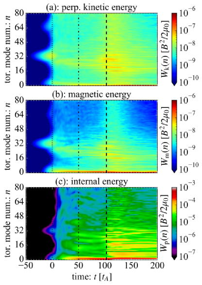
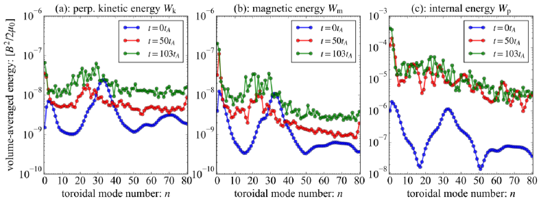
Figure 4: time evolution of energy spectra; (a): the perpendicular kinetic energy, (b): the magnetic energy and (c): the internal energy in the full torus case, where the dotted lines are at $t=0t_{A}$, the dash-dot lines are at an intermediate time between the two crashes $t=50t_{A}$, and the dashed lines are at $t=103t_{A}$, respectively.

Figure 5: toroidal mode spectra of the three system energies at $t=0t_{A}$ (blue), $t=50t_{A}$ (red), and $t=103t_{A}$ (green); (a) the perpendicular kinetic energy, (b) the magnetic energy, (c) the internal energy, respectively.

For generation mechanism of low-$n$ modes, time evolution of low-$n$ magnetic energies is shown in Fig. 6. In the early nonlinear phase before the first crash, the $n=0$ and low-$n$ magnetic energies develop with the growth rate almost twice of that of the $n=32$ magnetic energy. This indicates that the $n=0$ and low-$n$ magnetic energies are driven by nonlinear couplings among the RDBMs. After the first crash, the low-$n$ magnetic energies get saturated while the $n=0$ magnetic energy nonlinearly grows until the second crash, and the $n=0$ magnetic energy becomes a dominant component after the second crash. A detailed discussion on the generation mechanism of low-$n$ components of the magnetic energy after the first crash is given later with three-wave analyses of nonlinear terms.

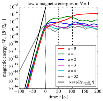
Figure 6: time evolution of low toroidal mode number components of magnetic energy in the full torus case, where the black dotted line is at $t=0t_{A}$, the black dash-dot line is at $t=50t_{A}$, the black dashed line is at $t=103t_{A}$, the gray curve is the time evolution of the initially most unstable $n=32$ component of magnetic energy, and the black sold line represents a curve with twice larger growth rate than that of the $n=32$ one.

Figure 7 shows the time evolution of pressure profiles on the $\zeta=0$ plane. At the first crash, fine scale pressure fluctuations driven by the RDBMs are poloidally localized in the two regions, upper left and lower right regions on the $q=2$ flux surface where the initial pressure gradient peak exists. After the first crash, pressure fluctuations expand out poloidally and finally cover over the flux surface at the second crash. This spatial structure can be related with $m/n=2/1$ magnetic fluctuations. Energy budgets of $n=1$ system energies are analyzed to clarify generation mechanism of $n=1$ magnetic fluctuations and magnetic field line tracing analyses are carried out to clarify the role of magnetic field fluctuations on ELM energy loss process.

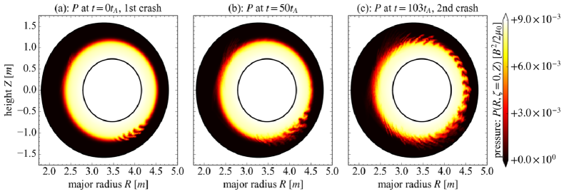
Figure 7: pressure profiles on $\zeta=0$-plane in cylindrical coordinates at (a): $t=0t_{A}$, (b): $t=50t_{A}$, and (c): $t=103t_{A}$, respectively.

The budget of $n=1$ internal energy Eq. (18) is summarized in Fig. 8(a). Here the terms with the superscript “li” transfer energy within $n=1$ components and the terms with the superscript “nl” transfer energy among all toroidal mode components, respectively. The $n=1$ internal energy is driven by the $E\times B$ convection term $T_{\rm p,PV}^{\rm nl}$ and its change rate becomes deeply negative after the second crash. The sum of contributions from the compression terms $T_{\rm p,CO}$ is a higher order term and is much smaller than the others. The compression terms however form energy channels between the other system energies and should be kept for self-consistent energy transfer in the simulated system.

The energy transfers between the $n=1$ internal energy $W_{\rm p}(t,n=1)$, perpendicular kinetic energy $W_{\rm k}(t,n=1)$ and magnetic energy $W_{\rm m}(t,n=1)$ are summarized in Fig. 8(b)-(d), where the terms with the same color construct energy transfer channels. The budget of $n=1$ parallel kinetic energy $W_{\rm v}(t,n=1)$ has not be shown since the parallel kinetic energy is weakly coupled only with the internal energy via parallel pressure compression terms $T_{\rm p,CV}^{\rm li}$ and $T_{\rm p,CV}^{\rm nl}$, and has little impact on the magnetic energy generation in this model.

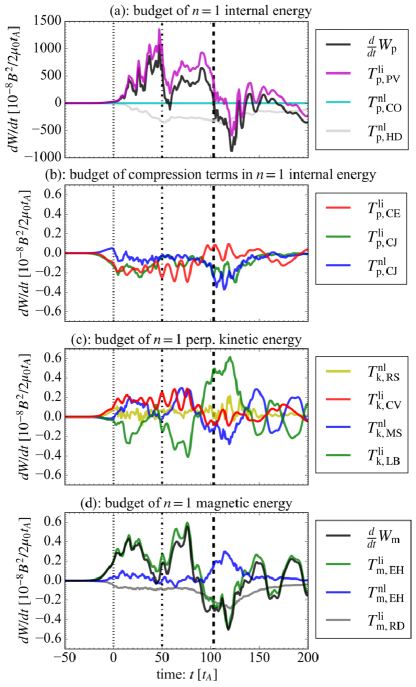
Figure 8: Time evolution of (a) the budget of $n=1$ internal energy equation, (b) the budget of the compression terms coupling with the perpendicular kinetic energy and the magnetic energy in $n=1$ internal energy equation, (c) the budget of $n=1$ perpendicular kinetic energy, and (d) the budget of $n=1$ magnetic energy, respectively. Here, the energy loss by numerical viscosity terms $T_{\rm k,VD}^{\rm li}$ and the change rate of $n=1$ kinetic energy $\frac{d}{dt}W_{\rm k}$ in Fig. 8(c) have not been plotted for readability, and the black dotted lines are $t=0t_{A}$, the black dash-dot lines are $t=50t_{A}$, and the black dashed lines are $t=103t_{A}$, respectively.

For the $n=1$ magnetic energy generation, the contribution from the $E\times B$ convection in the $n=1$ internal energy equation $T_{\rm p,PV}^{\rm nl}$ and that from the Maxwell stress in the $n=1$ perpendicular kinetic energy equation $T_{\rm k,MS}^{\rm nl}$ are positive after the first crash while the other nonlinear contributions are small till the second crash. Here the positive and negative signs indicate the energy gain and loss, respectively. It should be noted that nonlinear couplings by means of Poisson brackets in reduced MHD model generate the tearing parity components via nonlinear parity mixing Sato and Ishizawa (2017); Ishizawa, Kishimoto, and Nakamura (2019). The $n=1$ magnetic energy is mainly driven by the linear part of the electrostatic and electron Hall term $T_{\rm m,EH}^{\rm li}$ which cannot contribute to the parity mixing directly, but the $n=1$ pressure and electrostatic potential perturbations are driven by $T_{\rm p,PV}^{\rm nl}$ and $T_{\rm k,MS}^{\rm nl}$ which generate the tearing-parity components. Then, the tearing parity of the $n=1$ parallel magnetic potential is given by the linear combination of pressure and electrostatic potential via $T_{\rm m,EH}^{\rm li}$. This is consistent with the exponential growth of the $n=1$ magnetic energy with the growth rate almost twice larger than that of the $n=32$ magnetic energy at the early nonlinear phase. Our previous work Seto et al. (2023) also confirmed that the $n=1$ tearing parity is obtained after the second crash.

To clarify the nonlinear energy transfer channel driving the $n=1$ magnetic energy, three-wave analysis on the $E\times B$ convection term $T_{\rm p,PV}^{\rm nl}(t,n_{1},n_{2},n_{3})$ and that on the Maxwell stress term $T_{\rm k,MS}^{\rm nl}(t,n_{1},n_{2},n_{3})$,

$$T_{\rm p,PV}^{\rm nl}(t,n_{1},n_{2},n_{3}) = -\langle\frac{1}{2\beta_{*}}{P}_{1}^{n=n_{3}}\left[\phi^{n=n_{1}},P^{n=n_{2}}\right]\rangle_{V},$$ (28)

$$T_{\rm k,MS}^{\rm nl}(t,n_{1},n_{2},n_{3}) = -\langle{F}_{1}^{n=n_{3}}{B}_{0}\left[{A_{\parallel}}_{1}^{n=n_{1}},\frac{J_{\parallel}^{n=n_{2}}}{{B}_{0}}\right]\rangle_{V},$$ (29)

are applied with $n_{3}=1$ at $t=0t_{A}$, $t=50t_{A}$ and $t=103t_{A}$. Here, pairs of $n_{1}$ and $n_{2}$ satisfying $|n_{1}-n_{2}|=1$ can contribute to $n=1$ energy gains and the results are summarized in Fig. 9.

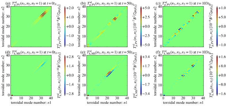
Figure 9: Three-wave analyses of the $E\times B$ convection term in the $n=1$ internal energy equation at (a): $t=0t_{A}$, (b): $t=50t_{A}$ and (c): $t=103t_{A}$, and three-wave analyses of the Maxwell stress term in the $n=1$ perpendicular kinetic energy equation at (d): $t=0t_{A}$, (e): $t=50t_{A}$ and (f): $t=103t_{A}$, respectively.

For the $E\times B$ convection term, pairs in the RDBMs have positive contributions to the $n=1$ internal energy at the first crash and pairs in the down-shifted middle-$n$ turbulence also have positive contributions to the $n=1$ internal energy at $t=50t_{A}$. At the second crash, a wide range of spectrum have positive and negative contributions to the $n=1$ internal energy. For the Maxwell stress, at the first crash and $t=50t_{A}$, the coupling with $(n_{1},n_{2})=(1,0)$ is the dominant positive contribution so that the $n=1$ perpendicular kinetic energy gets energy from $n=0$ and $n=1$ magnetic energy. Pairs in middle-$n$ modes satisfying $n_{1}-n_{2}=+1$ have negative contributions and those satisfying $n_{1}-n_{2}=-1$ have positive contributions at the first crash and $t=50t_{A}$. At the second crash, the coupling with $(n_{1},n_{2})=(1,0)$ has the large negative contribution so that the $n=1$ perpendicular kinetic energy gives energy to the $n=0$ and $n=1$ magnetic energies.

To understand the generation mechanism of the poloidally localized pressure fluctuations at the first crash in Fig. 7, spatio-temporal structure of the radial $E\times B$ heat flux $q^{\rm rad}_{E\times B}$ along $\zeta=0$ line on the $q=2$ flux surface and time evolution of Poincare plot of magnetic field lines are calculated, which are summarized in Fig. 10. Here the straight-field-line (SFL) poloidal angle $\vartheta$ in Fig. 10 is defined with the magnetic local pitch and the orthogonal poloidal angle $\theta$

$$\vartheta\equiv=\frac{1}{q}\int_{0}^{\theta}\frac{{\bm{B}}_{0}\cdot\nabla\zeta}{{\bm{B}}_{0}\cdot\nabla\theta}d\theta,$$ (30)

and the radial $E\times B$ heat flux $q^{\rm rad}_{E\times B}$ is also defined with the radial $E\times B$ flow $v^{\rm rad}_{E\times B}$,

$$v_{E\times B}^{\rm rad} = \bm{v}_{E\times B}\cdot h_{\psi}\nabla\psi=\frac{1}{B_{p}R}\frac{\partial\phi}{\partial z}-\frac{B_{t}}{B^{2}h_{\theta}}\frac{\partial\phi}{\partial y},$$ (31)

$$q_{E\times B}^{\rm rad} = P{v}_{E\times B}^{\rm rad}=P\left(\frac{1}{B_{p}R}\frac{\partial\phi}{\partial z}-\frac{B_{t}}{B^{2}h_{\theta}}\frac{\partial\phi}{\partial y}\right).$$ (32)

Figure 10 clearly shows that the $n=1$ magnetic perturbation forms $m/n=2/1$ magnetic islands at the first crash and the radial heat flux only exists the region with the stochastic magnetic field around the X-points of the $m/n=2/1$ magnetic islands. Here, the width of the stochastic region at the first crash seems to be determined by the location of X-points of $m/n=2/1$ and $m/n=8/4$ magnetic islands. The magnetic topology gets more stochastic with time since the higher harmonics of the $m/n=2/1$ magnetic islands develop on the $q=2$ rational surface and the magnetic island overlapping strongly enhance magnetic stochastisationDiamond et al. (1984). It is should be noted that the radial heat flux flows out from the X-point of higher harmonics of $m/n=2/1$ magnetic islands, which enhances energy loss level. In this simulation, the radial heat flux flows out from two X-points of $m/n=8/4$ magnetic island around $\vartheta/2\pi\sim 0.34~{}\mbox{and}~{}0.84$ at $t=50t_{A}$.

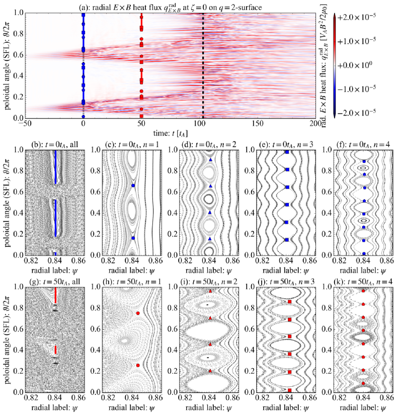
Figure 10: (a): spatio-temporal structure of radial heat flux by $E\times B$ convection on the $q=2$ flux surface, Poincare plots of magnetic field line at $t=0t_{A}$ including (b): all toroidal mode numbers of magnetic perturbations, (c): $n=1$ single mode, (d): $n=2$ single mode, (e): $n=3$ single mode, (f): $n=4$ single mode, and those at $t=50t_{A}$ including (g): all toroidal mode numbers of magnetic perturbations, (h): $n=1$ single mode, (i): $n=2$ single mode, (j): $n=3$ single mode, (k): $n=4$ single mode, respectively. Here the solid lines indicate the existing area of magnetic islands, and the circles, the triangles, the squares and the pentagons are the X-points of $m/n=2/1$, $m/n=4/2$, $m/n=6/3$, and $m/n=8/4$ magnetic islands at $t=0t_{A}$ (blue) and $t=50t_{A}$ (red), respectively.

The poloidal plot of total pressure and $E\times B$ flow components around the low magnetic field side of the X-points of the $m/n=2/1$ magnetic islands at the first and second crashes are summarized in Fig. 11. Here the magnetic islands are shown with the solid curves, and the poloidal $E\times B$ flow $v_{E\times B}^{\rm pol}$ and the 2D $E\times B$ flow $v_{E\times B}^{\rm 2D}$ are given by

$$v_{E\times B}^{\rm pol} = \bm{v}_{E\times B}\cdot h_{\theta}\nabla\theta=\frac{B_{t}B_{p}R}{{B}_{0}^{2}}\frac{\partial\phi}{\partial\psi},$$ (33)

$$v_{E\times B}^{\rm 2D} = \sqrt{(v_{E\times B}^{\rm rad})^{2}+(v_{E\times B}^{\rm pol})^{2}}.$$ (34)

At the first crash, the radial flow filaments are localized in the region without magnetic islands and the poloidal flow consisting of the small scale zonal flow and the large scale mean flow forms a laminar structure in the region with magnetic islands. The vortex flow pattern enhancing energy loss is therefore observed in the region without magnetic islands. At the second crash when the magnetic topology around the $q=2$ flux surface is fully stochastic, the pressure filaments expand poloidally as well as the radial flow filaments. The vortex pattern of 2D $E\times B$ flow therefore is formed over the domain and results in the increase of ELM energy loss. These results are consistent with the pressure profiles and the spatio-temporal analysis of radial $E\times B$ heat flux in Fig. 10. Here, an analysis of the causality between the magnetic stochastisation and the vortex flow pattern formation is left for a future work.

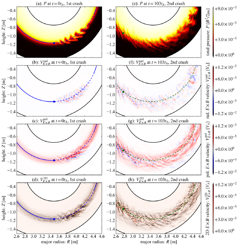
Figure 11: poloidal slices of (a) total pressure, (b) radial $E\times B$ flow, (c) poloidal $E\times B$ flow and (d) 2D velocity of $E\times B$ flow on the $\zeta=0$ plane at the first crash, and those of (e) total pressure, (f) radial $E\times B$ flow, (g) poloidal $E\times B$ flow and (h) 2D velocity of $E\times B$ flow on the $\zeta=0$ plane at the second crash, respectively. Here the dashed blue and green curves are the $q=2$ surface, the blue and green circles are the X-points of $m/n=2/1$ magnetic islands in the case where only $n=1$ magnetic perturbation is taken into account, and the solid blue curves are the region where the magnetic islands exist, respectively.

To clarify the trigger mechanism of two crashes, the three-wave analysis of the $E\times B$ convection term in the $n=0$ internal energy $T^{\rm nl}_{\rm p,PV}(t,n_{1}=n,n_{2}=n,n_{3}=0)$ is investigated, which is summarized in Fig. 12. Here the positive contribution enhances the $n=0$ pressure deformation. At $t=0t_{A}$, the middle-$n$ modes corresponding to the RDBMs have dominant contribution to the $n=0$ pressure deformation. At $t=50t_{A}$ and $t=103t_{A}$, a wide range of resonant modes with the down-shifted middle-$n$ mode have positive contributions to the $n=0$ pressure deformation. These results indicate that the first crash is triggered by the RDBMs and the second crash by the down-shifted middle-$n$ turbulence rather than low-$n$ modes. The low-$n$ modes have stabilization effects on the ELM crash.

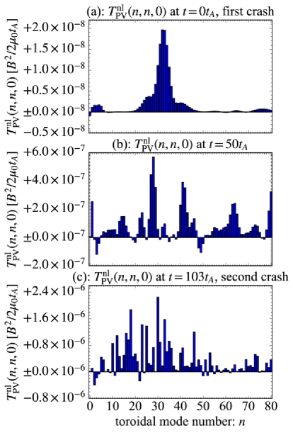
Figure 12: three-wave analysis of the $E\times B$ convection term in $n=0$ internal energy at (a): $t=0t_{A}$, (b): $t=50t_{A}$, and (c): $t=103t_{A}$, respectively.

Finally the impact of toroidal wedge numbers on the two-stage crash process is investigated for $N=1,2,4$. Figure 13 shows the impact of toroidal wedge numbers on the energy loss, where the result with $N=1$ is also plotted as a reference (see Fig. 3). It is found that the interval between the first and second crashes becomes shorter with the larger toroidal wedge number, namely $\Delta t=103t_{A}$ in the full torus case with $N=1$, $\Delta t=64t_{A}$ in the half torus case with $N=2$, and $\Delta t=3t_{A}$ in the quarter torus case with $N=4$. In the $N=4$ case where the two crashes occur at almost same timing, the RDBMs directly trigger the ELM crash, which is consistent with our previous work with the $1/5$-th torus wedge torus Seto et al. (2020).

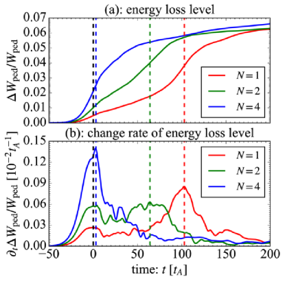
Figure 13: time evolution of (a) energy loss level and (b) its change rate for the $N=1$ case (red), the $N=2$ case (green), and the $N=4$ case (blue), respectively. Here the time labels are set to be $t=0t_{A}$ at the first crash and the timings of the second crash are highlighted with colored dashed lines.

To understand the reason why the toroidal wedge number has the impact on the crash process, we analyze spatio-temporal structure of the radial $E\times B$ convective heat flux $q^{\rm rad}_{E\times B}$ at the $\zeta=0$ line on the $q=2$ flux surface and time evolution of the magnetic field line topology, where the results in the $N=2$ case are shown in Fig. 14 and those in the $N=4$ torus case are in Fig. 15, respectively. In the $N=2$ case, the $m/n=4/2$ magnetic islands are generated in the early nonlinear phase ($t=-25t_{A}$). These magnetic islands have finer structure with more X-points and disappear faster compared with the $m/n=2/1$ magnetic islands in the $N=1$ case due to the magnetic island overlapping with higher harmonics, which leads to the faster second crash. In the $N=4$ case, the second crash occurs more rapidly. The $m/n=8/4$ magnetic islands are generated via nonlinear couplings in the early nonlinear phase ($t=-25t_{A}$), but they are already hidden in the sea of the stochasticity at the first crash. This is the reason why the two crashes occur almost simultaneously in the $N=4$ case. These results indicate that the toroidal wedge number affects the trigger dynamics of ELM crash via nonlinear interaction.

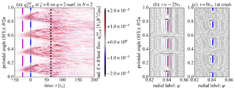
Figure 14: (a): spatio-temporal structure of radial heat flux by $E\times B$ flow on the $q=2$ flux surface, Poincare plot of magnetic field line including all toroidal mode component magnetic perturbation at (b): $t=-25t_{A}$ and (c): $t=0t_{A}$ in the half torus case $N=2$. Here the magenta lines are regions where magnetic islands exist at $t=-25t_{A}$ and the blue lines are those at $t=0t_{A}$.

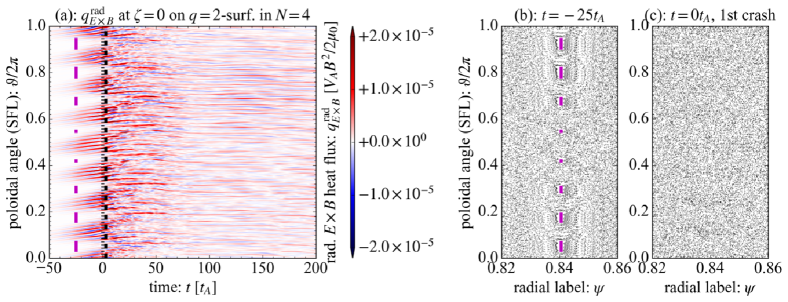
Figure 15: (a): spatio-temporal structure of radial heat flux by $E\times B$ flow on the $q=2$ flux surface, Poincare plot of magnetic field line including all toroidal mode component magnetic perturbation at (b): $t=-25t_{A}$ and (c) $t=0t_{A}$ in the quarter torus case $N=4$. Here the magenta lines are regions where magnetic islands exist at $t=-25t_{A}$.

IV Summary and Discussions

In order to understand the crash mechanism of the RDBM-driven ELM, we have conducted the analyses on simulation data in the full torus domain and compared with those in half and quarter torus domains.

In the early nonlinear phase, the first crash is triggered by the linearly unstable RDBMs and the $m/n=2/1$ magnetic islands are nonlinearly excited by the parity mixing Sato and Ishizawa (2017); Ishizawa, Kishimoto, and Nakamura (2019) via nonlinear couplings of the RDBMs. Simultaneously, the middle-$n$ RDBM turbulence develops but is poloidally localized around X-points of the magnetic islands, leading to the small energy loss. The $m/n=2/1$ magnetic islands have the stabilization effect on the RDBM-driven ELM crash.

The second crash then occurs in the late nonlinear phase. The higher harmonics of $m/n=2/1$ magnetic islands are also excited around the $q=2$ surface via nonlinear couplings among the middle-$n$ turbulence. Since the turbulence develops from some of their X-points, it expands out poloidally. The second crash is triggered by the middle-$n$ turbulence when the turbulence covers the whole poloidal region.

Finally, the scan of toroidal wedge number $N$ has revealed that the interval between the first and second crashes becomes shorter with the larger toroidal wedge number, and the two crashes occur almost simultaneously in the quarter torus case with $N=4$. This is because that the finer magnetic islands with $m/n=2N/N$ are generated in the early nonlinear phase and the magnetic stochastisation occurs faster for the larger toroidal wedge number. These results indicate that nonlinear interactions of all channels in the full torus domain can significantly affect the trigger dynamics of ELMs driven by the RDBMs.

It should be noted again that the linearized parallel heat diffusion term and the constant heat diffusivity and hyper resistivity have been employed in this work. The anomalous heat transport Rechester and Rosenbluth (1978) and hyper resistivity Kaw, Valeo, and Rutherford (1979) by magnetic stochastisation have not been taken into account. With these anomalous effects, a hyper-exponential growth of the low-$n$ fluctuations Itoh et al. (1998) and an increase of the energy loss in the stochastic regions Rhee et al. (2015) may be expected. It is left for a future work.

Within the context of the full torus case, it becomes evident that the nonlinear coupling between modes during the first crash phase assumes a pivotal role. This coupling not only leads to the deformation of the magnetic field configuration but also results in the disruption of magnetic flux surfaces through reconnections. Furthermore, it facilitates the conversion of the perpendicular kinetic energy into the magnetic energy, effectively postponing the substantial loss of the internal energy.

It’s imperative to underscore that extensive internal energy loss, large ELM crashes, and significant inter-energy transport predominantly arise from the intricate overlaps of fine magnetic islands, rather than the mere presence of low-$n$ magnetic islands. Low-$n$ islands still maintain a relatively modest ratio between the volume of stochastic regions near the X-points and the confined regions inside the island. It is within these stochastic regions that substantial internal energy transport takes place.

As the number of fine islands continues to increase and they begin to overlap, this ratio escalates, leading to heightened internal energy transport and ultimately culminating in the occurrence of large ELM crashes. This dynamic likely accounts for the observed variation in crash behavior for different toroidal wedge numbers, while the ultimate size of the ELM remains relatively consistent.

References

- Zohm (1996) H. Zohm, “The physics of edge localized modes (ELMs) and their role in power and particle exhaust,” Plasma Physics and Controlled Fusion 38, 1213–1223 (1996).
- Wagner et al. (1982) F. Wagner, G. Becker, K. Behringer, D. Campbell, A. Eberhagen, W. Engelhardt, G. Fussmann, O. Gehre, J. Gernhardt, G. v. Gierke, G. Haas, M. Huang, F. Karger, M. Keilhacker, O. Klüber, M. Kornherr, K. Lackner, G. Lisitano, G. G. Lister, H. M. Mayer, D. Meisel, E. R. Müller, H. Murmann, H. Niedermeyer, W. Poschenrieder, H. Rapp, H. Röhr, F. Schneider, G. Siller, E. Speth, A. Stäbler, K. H. Steuer, G. Venus, O. Vollmer, and Z. Yü, “Regime of Improved Confinement and High Beta in Neutral-Beam-Heated Divertor Discharges of the ASDEX Tokamak,” Physical Review Letters 49, 1408–1412 (1982).
- Kukushkin et al. (2011) A. Kukushkin, H. Pacher, V. Kotov, G. Pacher, and D. Reiter, “Finalizing the iter divertor design: The key role of solps modeling,” Fusion Engineering and Design 86, 2865–2873 (2011).
- Gunn et al. (2017) J. Gunn, S. Carpentier-Chouchana, F. Escourbiac, T. Hirai, S. Panayotis, R. Pitts, Y. Corre, R. Dejarnac, M. Firdaouss, M. Kočan, M. Komm, A. Kukushkin, P. Languille, M. Missirlian, W. Zhao, and G. Zhong, “Surface heat loads on the ITER divertor vertical targets,” Nuclear Fusion 57, 046025 (2017).
- Asakura et al. (2021) N. Asakura, K. Hoshino, Y. Homma, and Y. Sakamoto, “Simulation studies of divertor detachment and critical power exhaust parameters for japanese demo design,” Nuclear Materials and Energy 26, 100864 (2021).
- Huysmans and Czarny (2007) G. T. A. Huysmans and O. Czarny, “MHD stability in X-point geometry: simulation of ELMs,” Nuclear Fusion 47, 659–666 (2007).
- Czarny and Huysmans (2008) O. Czarny and G. Huysmans, “Bézier surfaces and finite elements for MHD simulations,” Journal of Computational Physics 227, 7423–7445 (2008).
- Hoelzl et al. (2021) M. Hoelzl, G. Huijsmans, S. Pamela, M. Bécoulet, E. Nardon, F. Artola, B. Nkonga, C. Atanasiu, V. Bandaru, A. Bhole, D. Bonfiglio, A. Cathey, O. Czarny, A. Dvornova, T. Fehér, A. Fil, E. Franck, S. Futatani, M. Gruca, H. Guillard, J. Haverkort, I. Holod, D. Hu, S. Kim, S. Korving, L. Kos, I. Krebs, L. Kripner, G. Latu, F. Liu, P. Merkel, D. Meshcheriakov, V. Mitterauer, S. Mochalskyy, J. Morales, R. Nies, N. Nikulsin, F. Orain, J. Pratt, R. Ramasamy, P. Ramet, C. Reux, K. Särkimäki, N. Schwarz, P. S. Verma, S. Smith, C. Sommariva, E. Strumberger, D. van Vugt, M. Verbeek, E. Westerhof, F. Wieschollek, and J. Zielinski, “The JOREK non-linear extended MHD code and applications to large-scale instabilities and their control in magnetically confined fusion plasmas,” Nuclear Fusion 61, 065001 (2021).
- Sovinec et al. (2004) C. R. Sovinec, A. H. Glasser, T. A. Gianakon, D. C. Barnes, R. A. Nebel, S. E. Kruger, D. D. Schnack, S. J. Plimpton, A. Tarditi, and M. S. Chu, “Nonlinear magnetohydrodynamics simulation using high-order finite elements,” Journal of Computational Physics 195, 355–386 (2004).
- Ferraro, Jardin, and Snyder (2010) N. M. Ferraro, S. C. Jardin, and P. B. Snyder, “Ideal and resistive edge stability calculations with M3D-C1,” Physics of Plasmas 17, 102508–11 (2010).
- Wingen et al. (2015) A. Wingen, N. M. Ferraro, M. W. Shafer, E. A. Unterberg, J. M. Canik, T. E. Evans, D. L. Hillis, S. P. Hirshman, S. K. Seal, P. B. Snyder, and A. C. Sontag, “Connection between plasma response and resonant magnetic perturbation (RMP) edge localized mode (ELM) suppression in DIII-d,” Plasma Physics and Controlled Fusion 57, 104006 (2015).
- Todo and Sato (1998) Y. Todo and T. Sato, “Linear and nonlinear particle-magnetohydrodynamic simulations of the toroidal Alfvén eigenmode,” Physics of Plasmas 5, 1321–1327 (1998), https://pubs.aip.org/aip/pop/article-pdf/5/5/1321/12478284/1321_1_online.pdf .
- Todo et al. (2017) Y. Todo, R. Seki, D. A. Spong, H. Wang, Y. Suzuki, S. Yamamoto, N. Nakajima, and M. Osakabe, “Comprehensive magnetohydrodynamic hybrid simulations of fast ion driven instabilities in a Large Helical Device experiment,” Physics of Plasmas 24, 081203 (2017), https://pubs.aip.org/aip/pop/article-pdf/doi/10.1063/1.4997529/15644384/081203_1_online.pdf .
- Rivero Rodriguez et al. (2023) J. F. Rivero Rodriguez, J. Galdon-Quiroga, J. Dominguez-Palacios, M. Garcia-Munoz, D. GarcÃa-Vallejo, J. Gonzalez Martin, K. G. McClements, L. Sanchis, K. Särkimäki, A. Snicker, Y. Todo, L. Velarde, and E. Viezzer, “Transport and acceleration mechanism of fast ions during edge localized modes in asdex upgrade,” Nuclear Fusion (2023).
- Dudson et al. (2009) B. D. Dudson, M. V. Umansky, X. Q. Xu, P. B. Snyder, and H. R. Wilson, “BOUT++: A framework for parallel plasma fluid simulations,” Computer Physics Communications 180, 1467–1480 (2009).
- Xu et al. (2010) X. Q. Xu, B. Dudson, P. B. Snyder, M. V. Umansky, and H. Wilson, “Nonlinear Simulations of Peeling-Ballooning Modes with Anomalous Electron Viscosity and their Role in Edge Localized Mode Crashes,” Physical Review Letters 105, 949–4 (2010).
- Zhu et al. (2021) B. Zhu, H. Seto, X. qiao Xu, and M. Yagi, “Drift reduced landau fluid model for magnetized plasma turbulence simulations in bout++ framework,” Computer Physics Communications 267, 108079 (2021).
- D’haeseleer et al. (1991) W. D. D’haeseleer, W. N. G. Hitchon, J. D. Callen, and J. L. Shohet, Flux Coordinates and Magnetic Field Structure (Springer-Verlag, 1991).
- Beer, Cowley, and Hammett (1995) M. A. Beer, S. C. Cowley, and G. W. Hammett, “Field-aligned coordinates for nonlinear simulations of tokamak turbulence,” Physics of Plasmas 2, 2687–2700 (1995).
- Seto et al. (2023) H. Seto, B. D. Dudson, X.-Q. Xu, and M. Yagi, “A bout++ extension for full annular tokamak edge mhd and turbulence simulations,” Computer Physics Communications 283, 108568 (2023).
- Evans et al. (2004) T. E. Evans, R. A. Moyer, P. R. Thomas, J. G. Watkins, T. H. Osborne, J. A. Boedo, E. J. Doyle, M. E. Fenstermacher, K. H. Finken, R. J. Groebner, M. Groth, J. H. Harris, R. J. La Haye, C. J. Lasnier, S. Masuzaki, N. Ohyabu, D. G. Pretty, T. L. Rhodes, H. Reimerdes, D. L. Rudakov, M. J. Schaffer, G. Wang, and L. Zeng, “Suppression of large edge-localized modes in high-confinement diii-d plasmas with a stochastic magnetic boundary,” Phys. Rev. Lett. 92, 235003 (2004).
- Orain et al. (2013) F. Orain, M. Becoulet, G. Dif-Pradalier, G. Huijsmans, S. Pamela, E. Nardon, C. Passeron, G. Latu, V. Grandgirard, A. Fil, A. Ratnani, I. Chapman, A. Kirk, A. Thornton, M. Hoelzl, and P. Cahyna, “Non-linear magnetohydrodynamic modeling of plasma response to resonant magnetic perturbations,” Physics of Plasmas 20, 102510–23 (2013).
- Burrell et al. (2002) K. H. Burrell, M. E. Austin, D. P. Brennan, J. C. DeBoo, E. J. Doyle, P. Gohil, C. M. Greenfield, R. J. Groebner, L. L. Lao, T. C. Luce, M. A. Makowski, G. R. McKee, R. A. Moyer, T. H. Osborne, M. Porkolab, T. L. Rhodes, J. C. Rost, M. J. Schaffer, B. W. Stallard, E. J. Strait, M. R. Wade, G. Wang, J. G. Watkins, W. P. West, and L. Zeng, “Quiescent h-mode plasmas in the DIII-d tokamak,” Plasma Physics and Controlled Fusion 44, A253–A263 (2002).
- Liu et al. (2015) F. Liu, G. Huijsmans, A. Loarte, A. Garofalo, W. Solomon, P. Snyder, M. Hoelzl, and L. Zeng, “Nonlinear MHD simulations of quiescent h-mode plasmas in DIII-d,” Nuclear Fusion 55, 113002 (2015).
- Xi, Xu, and Diamond (2014) P. W. Xi, X. Q. Xu, and P. H. Diamond, “Phase Dynamics Criterion for Fast Relaxation of High-Confinement-Mode Plasmas,” Physical Review Letters 112, 085001–5 (2014).
- Kim et al. (2017) K. Kim, C. S. Chang, J. Seo, S. Ku, and W. Choe, “What happens to full-f gyrokinetic transport and turbulence in a toroidal wedge simulation?” Physics of Plasmas 24, 012306 (2017), https://pubs.aip.org/aip/pop/article-pdf/doi/10.1063/1.4974777/16130176/012306_1_online.pdf .
- Seto et al. (2020) H. Seto, X. Xu, B. D. Dudson, and M. Yagi, “Impact of equilibrium radial electric field on energy loss process after pedestal collapse,” Contributions to Plasma Physics 60, e201900158 (2020), https://onlinelibrary.wiley.com/doi/pdf/10.1002/ctpp.201900158 .
- Chang and Callen (1992) Z. Chang and J. D. Callen, “Generalized gyroviscous force and its effect on the momentum balance equation,” Physics of Fluids B: Plasma Physics 4, 1766–1771 (1992).
- Itoh and Itoh (1996) K. Itoh and S.-I. Itoh, “The role of the electric field in confinement,” Plasma Physics and Controlled Fusion 38, 1 (1996).
- Rechester and Rosenbluth (1978) A. B. Rechester and M. N. Rosenbluth, “Electron heat transport in a tokamak with destroyed magnetic surfaces,” Phys. Rev. Lett. 40, 38–41 (1978).
- Kaw, Valeo, and Rutherford (1979) P. K. Kaw, E. J. Valeo, and P. H. Rutherford, “Tearing modes in a plasma with magnetic braiding,” Phys. Rev. Lett. 43, 1398–1401 (1979).
- Wilson et al. (2002) H. R. Wilson, P. B. Snyder, G. T. A. Huysmans, and R. L. Miller, “Numerical studies of edge localized instabilities in tokamaks,” Physics of Plasmas 9, 1277–1286 (2002), https://doi.org/10.1063/1.1459058 .
- Snyder et al. (2002) P. B. Snyder, H. R. Wilson, J. R. Ferron, L. L. Lao, A. W. Leonard, T. H. Osborne, A. D. Turnbull, D. Mossessian, M. Murakami, and X. Q. Xu, “Edge localized modes and the pedestal: A model based on coupled peeling–ballooning modes,” Physics of Plasmas 9, 2037–2043 (2002).
- Miller and Vandam (1987) R. L. Miller and J. W. Vandam, “Hot Particle Stabilization of Ballooning Modes in Tokamaks,” Nuclear Fusion 27, 2101–2112 (1987).
- Burke et al. (2010) B. J. Burke, S. E. Kruger, C. C. Hegna, P. Zhu, P. B. Snyder, C. R. Sovinec, and E. C. Howell, “Edge localized linear ideal magnetohydrodynamic instability studies in an extended-magnetohydrodynamic code,” Physics of Plasmas 17, 032103–12 (2010).
- Seto et al. (2019) H. Seto, X. Q. Xu, B. D. Dudson, and M. Yagi, “Interplay between fluctuation driven toroidal axisymmetric flows and resistive ballooning mode turbulence,” Physics of Plasmas 26, 052507–16 (2019).
- Sato and Ishizawa (2017) M. Sato and A. Ishizawa, “Nonlinear parity mixtures controlling the propagation of interchange modes,” Physics of Plasmas 24, 082501 (2017), https://pubs.aip.org/aip/pop/article-pdf/doi/10.1063/1.4993472/15647332/082501_1_online.pdf .
- Ishizawa, Kishimoto, and Nakamura (2019) A. Ishizawa, Y. Kishimoto, and Y. Nakamura, “Multi-scale interactions between turbulence and magnetic islands and parity mixture—a review,” Plasma Physics and Controlled Fusion 61, 054006 (2019).
- Diamond et al. (1984) P. H. Diamond, R. D. Hazeltine, Z. G. An, B. A. Carreras, and H. R. Hicks, “Theory of anomalous tearing mode growth and the major tokamak disruption,” The Physics of Fluids 27, 1449–1462 (1984), https://pubs.aip.org/aip/pfl/article-pdf/27/6/1449/12612095/1449_1_online.pdf .
- Itoh et al. (1998) S.-I. Itoh, K. Itoh, H. Zushi, and A. Fukuyama, “Physics of collapse events in toroidal plasmas,” Plasma Physics and Controlled Fusion 40, 879 (1998).
- Rhee et al. (2015) T. Rhee, S. Kim, H. Jhang, G. Park, and R. Singh, “A mechanism for magnetic field stochastization and energy release during an edge pedestal collapse,” Nuclear Fusion 55, 032004 (2015).