Updatable Estimation in Generalized Linear Models with Missing Response

Abstract

This paper develops an updatable inverse probability weighting (UIPW) estimation for the generalized linear models with response missing at random in streaming data sets. A two-step online updating algorithm is provided for the proposed method. In the first step we construct an updatable estimator for the parameter in propensity function and hence obtain an updatable estimator of the propensity function; in the second step we propose an UIPW estimator with the inverse of the updating propensity function value at each observation as the weight for estimating the parameter of interest. The UIPW estimation is universally applicable due to its relaxation on the constraint on the number of data batches. It is shown that the proposed estimator is consistent and asymptotically normal with the same asymptotic variance as that of the oracle estimator, and hence the oracle property is obtained. The finite sample performance of the proposed estimator is illustrated by the simulation and real data analysis. All numerical studies confirm that the UIPW estimator performs as well as the batch learner.

Keywords: Generalized linear model; Streaming data sets; Missing response; Updatable inverse probability weighting.

1 Introduction

With the development of modern science and technology, massive data sets arise in various fields. It not only presents opportunities, but also brings challenges, such as the difficulty of storing on standard computers and the insufficient computation speed of traditional algorithms. Until now, the major strategies to meet challenges have been researched by many statisticians, most of which can be divided into the three categories: sub-sampling (Liang et al., 2013; Kleiner et al., 2014; Ping et al., 2015), divide and conquer (Lin & Xi, 2011; Scott et al., 2016; Chen & Xie, 2014; Song & Liang, 2014; Pillonetto et al., 2019) and the online updating (Schifano et al, 2016; Wang et al., 2018; Xue et al., 2020; Luo & Song, 2020). However, the online updating is basically different from the others because the streaming data set is a special data type in the emerging field of ”big data”. More specifically, in the streaming data set, the data arrive in streams and chunks sequentially. So the statistical method should be of online updating framework, without storage requirement for historical data.

The stochastic gradient descent (SGD) algorithm proposed by Robbins & Monro (1951) is a well-known iterative algorithm. Since the SGD algorithm updates the estimation with one data point at each time, it coincides with the mechanism of how data are observed in streaming data sets and becomes a natural solution to the online estimation. The SGD algorithm has been developed by statisticians with many improved versions, such as averaged implicit SGD (AISGD) (Toulis et al., 2014) and SGD-QN (Bordes et al., 2009). The online second-order method is another popular approach for handling streaming data sets, such as Amari et al. (2000) proposed the online Newton step. Furthermore, Chen et al. (2021) proposed an SGD-based online algorithm that can make decisions and update the decision rule online. In addition to the SGD-based online algorithm, Schifano et al. (2016) extended the cumulative estimating equation (CEE) estimator (Lin & Xi, 2011) and proposed the cumulatively updated estimating equation (CUEE) estimator. The CUEE estimator had been shown to be superior to other divide-and-conquer or online-updated estimators in terms of bias and mean squared error. However, the CUEE estimator sacrifices application value for the oracle property and estimation consistency. For example, the total number of streaming data sets is usually constrained by $K=O\left(N^{c}_{K}\right)$, where $0\textless c\textless 1$ is a constant, $N_{K}$ is the number of total data and $K$ is the total number of the data batches. This constraint means that the total number of the data batches cannot be very large. Lin & Zhang (2002) proposed a two-sample empirical Euclidean penalty likelihood method based on historical empirical estimation and current empirical information. Luo & Song (2020) proposed the renewable estimation (RE) through an incremental updating algorithm which can relax the constraint. But the above methods only focused on the case of complete data.

As Zhu et al. (2019) pointed out, in the era of big data, it is more likely to encounter incomplete observations. Imputation (Rubin, 1987; 1996) is a widely adopted approach for dealing with missing data. Wang (2008) proposed two nonparametric probability density estimations: inverse probability weighted estimation and the regression calibration density estimation. However, the estimating methods faced the challenge of curse of dimensionality. Hu et al. (2010, 2012) considered dimension reduction in estimation of response mean to avoid the curse of dimensionality. Based on the kernel smoothing and sieve method, Wang et al. (2021) developed two distributed nonparametric imputation methods, which extended the divide and conquer strategy to missing response problems. However, applying these imputation methods directly to the streaming data set is inappropriate (Syavasya & Lakshmi, 2022). To handle the missing data in the streaming data set, Wellenzohn et al. (2017) proposed Top-k Case Matching (TKCM) model. It consistently imputes the missing data and retains accuracy when there is a block of missing data. Peng et al. (2019) developed Incremental Space-Time based Model (ISTM) to impute the missing data in the streaming data set. Inverse probability weighting (IPW) (Horvitz & Thompson, 1952; Robins et al., 1994) is another popular approach for handling missing data. The inverse probability weighted method is applied to missing response problem to define M-estimators in Wang (2007). However, the existing IPW approaches for handling missing data are of the offline framework. How to use IPW approach to deal with the missing data in streaming data sets is a significant problem. To the best of our knowledge, there is little relevant literature to solve it. It is desired to develop online updating IPW estimation approaches and algorithms.

In this paper, we propose an online updating IPW estimation approach for the generalized linear model (GLM) (McCullagh & Nelder, 1983) in the presence of missing response. The proposed approach is developed with the commonly used IPW approach. Our contributions include the followings:

• A two-step online updating approach is proposed such that both the inverse probability weights and the estimator of the parameter of interest can update simultaneously;

• We establish the asymptotic property of the updatable estimator without the condition $K=O(N_{K}^{c}),0\textless c\textless 1$;

• Extend the proposed approach to the heterogeneous streaming data set. We get the efficient score function by the projection method, and then use a two-step online updating approach to get the online updating estimation.

The remainder of this paper is organized as follows. In Section 2, the UIPW estimation is proposed to construct the updatable estimator in the streaming data set with missing response for the GLM, via a two-step online updating algorithm. The theoretical properties of the updatable estimator are investigated. We extend the UIPW estimation to the heterogeneous streaming data set in Section 3 with an efficient UIPW (EUIPW) estimation. The main simulation studies and real data analysis are provided in Section 4 to evaluate the proposed method. Technical details are provided in Appendix.

2 Updatable inverse probability weighting estimation

2.1 Methodology

Let $W=(Y,X^{\top})^{\top}$ denote the full variable vector and $\boldsymbol{\beta}\in\boldsymbol{\Theta}_{\boldsymbol{\beta}}$ denote the $p$-dimensional parameter vector of interest with true value $\boldsymbol{\beta}^{0}$, where $Y$ is the response, $X\in\mathbb{R}^{p}$ is the associated covariate. In the complete case, for the GLM with $g(E[Y|X])=X^{\top}\boldsymbol{\beta}$, we assume that all the data $W_{i}=(Y_{i},X_{i}^{\top})^{\top}$ for $i=1,2,\ldots,n$ are independent and identically distributed and follow exponential family distribution with the probability density function (PDF)

$$f\left(y;\eta,\phi\right)=\exp\left\{\frac{y\eta-b\left(\eta\right)}{\phi}+c\left(y,\phi\right)\right\},$$ (1)

where $\phi$ is the dispersion parameter. Suppose that $\eta=\eta(x^{\top}\boldsymbol{\beta})$ is a monotone differentiable function. In the GLM, we have the following properties:

$$\begin{split}&\frac{\partial b(\eta(x^{\top}\boldsymbol{\beta}))}{\partial\eta(x^{\top}\boldsymbol{\beta})}=\mu,\text{ }\frac{\partial\mu}{\partial\eta(x^{\top}\boldsymbol{\beta})}=v(\mu),\\ &\frac{\partial\eta(x^{\top}\boldsymbol{\beta})}{\partial\boldsymbol{\beta}}=\frac{\partial\eta(x^{\top}\boldsymbol{\beta})}{\partial\mu}\frac{\partial\mu}{\partial g(\mu)}\frac{\partial g(\mu)}{\partial\boldsymbol{\beta}}=[v(\mu)g_{\mu}(\mu)]^{-1}x^{\top},\end{split}$$ (2)

where $\mu=E[Y|X=x]$, $v(\mu)$ is the known unit variance function defined as $Var(Y|X=x)=\phi v\left(\mu\right)$ and $g_{\mu}(\cdot)$ is the derivative of $g(\cdot)$ with respect to $\mu$. We write the associated log-likelihood function as:

$$\ell\left(\boldsymbol{\beta},\phi;\mathchoice{\hbox{\boldmath$\displaystyle W$}}{\hbox{\boldmath$\textstyle W$}}{\hbox{\boldmath$\scriptstyle W$}}{\hbox{\boldmath$\scriptscriptstyle W$}}_{n}\right)=\frac{1}{n}\sum_{i=1}^{n}\log f\left(Y_{i};X_{i},\boldsymbol{\beta},\phi\right)=\frac{1}{n}\sum_{i=1}^{n}\left\{\frac{Y_{i}\eta(X_{i}^{\top}\boldsymbol{\beta})-b\left(\eta(X_{i}^{\top}\boldsymbol{\beta})\right)}{\phi}+c\left(Y_{i},\phi\right)\right\},$$

where $\mathchoice{\hbox{\boldmath$\displaystyle W$}}{\hbox{\boldmath$\textstyle W$}}{\hbox{\boldmath$\scriptstyle W$}}{\hbox{\boldmath$\scriptscriptstyle W$}}_{n}=(W_{1},\ldots,W_{n})$. Maximizing $\ell\left(\boldsymbol{\beta},\phi;\mathchoice{\hbox{\boldmath$\displaystyle W$}}{\hbox{\boldmath$\textstyle W$}}{\hbox{\boldmath$\scriptstyle W$}}{\hbox{\boldmath$\scriptscriptstyle W$}}_{n}\right)$ is equivalent to maximizing $(1/n)\sum_{i=1}^{n}\{Y_{i}\eta(X_{i}^{\top}\boldsymbol{\beta})-b\left(\eta(X_{i}^{\top}\boldsymbol{\beta})\right)\}$ in $\ell\left(\boldsymbol{\beta},\phi;\mathchoice{\hbox{\boldmath$\displaystyle W$}}{\hbox{\boldmath$\textstyle W$}}{\hbox{\boldmath$\scriptstyle W$}}{\hbox{\boldmath$\scriptscriptstyle W$}}_{n}\right)$ with respect to $\boldsymbol{\beta}$. According to (2), the corresponding score function is $(1/n)\sum_{i=1}^{n}(Y_{i}-\mu_{i})[v(\mu_{i})g_{\mu}(\mu_{i})]^{-1}X_{i}^{\top}$.

In the presence of missing data, we assume the response $Y$ is subject to missingness, but the covariate $X$ is fully observed. Let $\delta$ denote the indicator of observing $Y$, i.e., $\delta=1$ if $Y$ is observed and $\delta=0$ otherwise. The observed data are $n$ independent and identically distributed copies of $(\delta,Y,X^{\top})$. We assume the response $Y$ is missing at random (MAR) (Rubin, 1976), that is

$$P(\delta=1|Y,X)=P(\delta=1|X),$$ (3)

which means that the response is missing depending on covariates only but not on itself.

Let $\pi(x)=P(\delta=1|X=x)$. However, in most situations, we need to deduce $\pi(X)$ based on the data. In particular, we generally can posit a model for $P(\delta=1|X)$; for example, a full parametric model $\pi(X;\boldsymbol{\alpha})$, where $\pi(\cdot;\cdot)$ is a known function, but $\boldsymbol{\alpha}\in\boldsymbol{\Theta}_{\boldsymbol{\alpha}}$ is an unknown parameter vector. With $\boldsymbol{\alpha}$ estimated by $\hat{\boldsymbol{\alpha}}$, the IPW estimator for $\boldsymbol{\beta}$ can be obtained according to Horvitz & Thompson (1952).

We consider the case where the samples arrive sequentially in chunks and the response is missing at random. With slightly abusing the notation, let $W=(\delta,Y,X^{\top})^{\top}$. The series of $k$ batches of data are denoted by $W_{1}=(\delta_{1},Y_{1},X_{1}^{\top})^{\top},\ldots,$
$W_{N_{k}}=(\delta_{N_{k}},Y_{N_{k}},X_{N_{k}}^{\top})^{\top}$, where $W_{i}$ are i.i.d. copies of $W$, totally $N_{k}$ observations available. For $j=1,\ldots,k,\ldots$, let $\boldsymbol{d}_{j}=(W_{i}:i\in\mathchoice{\hbox{\boldmath$\displaystyle i$}}{\hbox{\boldmath$\textstyle i$}}{\hbox{\boldmath$\scriptstyle i$}}{\hbox{\boldmath$\scriptscriptstyle i$}}_{j})$ be sequential data sets with the index sets $\mathchoice{\hbox{\boldmath$\displaystyle i$}}{\hbox{\boldmath$\textstyle i$}}{\hbox{\boldmath$\scriptstyle i$}}{\hbox{\boldmath$\scriptscriptstyle i$}}_{j}$ defined by $\mathchoice{\hbox{\boldmath$\displaystyle i$}}{\hbox{\boldmath$\textstyle i$}}{\hbox{\boldmath$\scriptstyle i$}}{\hbox{\boldmath$\scriptscriptstyle i$}}_{j}=\{N_{j-1}+1,\ldots,N_{j-1}+n_{j}\}$ with $N_{0}=0$ and $N_{k-1}+n_{k}=N_{k}$. When the $k$-th batch of data arrives, consider the IPW approach, for any $j\in\{1,\ldots,k\}$, the score function on the $j$-th batch of data is

$$\mathbf{S}(\boldsymbol{\beta}|\mathchoice{\hbox{\boldmath$\displaystyle d$}}{\hbox{\boldmath$\textstyle d$}}{\hbox{\boldmath$\scriptstyle d$}}{\hbox{\boldmath$\scriptscriptstyle d$}}_{j},\boldsymbol{\alpha})=\frac{1}{n_{j}}\sum_{i\in\mathchoice{\hbox{\boldmath$\displaystyle i$}}{\hbox{\boldmath$\textstyle i$}}{\hbox{\boldmath$\scriptstyle i$}}{\hbox{\boldmath$\scriptscriptstyle i$}}_{j}}S(W_{i};\boldsymbol{\beta},\boldsymbol{\alpha})=\frac{1}{n_{j}}\sum_{i\in\mathchoice{\hbox{\boldmath$\displaystyle i$}}{\hbox{\boldmath$\textstyle i$}}{\hbox{\boldmath$\scriptstyle i$}}{\hbox{\boldmath$\scriptscriptstyle i$}}_{j}}\frac{\delta_{i}}{\pi(X_{i};\boldsymbol{\alpha})}(Y_{i}-\mu_{i})[v(\mu_{i})g_{\mu}(\mu_{i})]^{-1}X_{i}^{\top},$$

Our goal is to construct the updatable estimator of $\boldsymbol{\beta}$ under the above settings. To this end, the first task is to obtain the online updating estimation of the unknown parameter vector $\textstyle\alpha$ in the propensity function $\pi(X;\boldsymbol{\alpha})$. Note that according to the binomial distribution, the log-likelihood function for $\textstyle\alpha$ on the $j$-th batch of data for any $j\in\{1,\ldots,k\}$ is

$$\frac{1}{n_{j}}\sum_{i\in\mathchoice{\hbox{\boldmath$\displaystyle i$}}{\hbox{\boldmath$\textstyle i$}}{\hbox{\boldmath$\scriptstyle i$}}{\hbox{\boldmath$\scriptscriptstyle i$}}_{j}}\log\bigg{\{}\pi(X_{i};\boldsymbol{\alpha})^{\delta_{i}}\big{[}1-\pi(X_{i};\boldsymbol{\alpha})\big{]}^{(1-\delta_{i})}\bigg{\}}.$$

Thus, the corresponding estimating function on the $j$-th batch of data $\boldsymbol{d}_{j}$ is

$$\mathbf{V}(\boldsymbol{\delta}_{j};\mathbf{X}_{j},\boldsymbol{\alpha})=\frac{1}{n_{j}}\sum_{i\in\mathchoice{\hbox{\boldmath$\displaystyle i$}}{\hbox{\boldmath$\textstyle i$}}{\hbox{\boldmath$\scriptstyle i$}}{\hbox{\boldmath$\scriptscriptstyle i$}}_{j}}V(\delta_{i};X_{i},\boldsymbol{\alpha})=\frac{1}{n_{j}}\sum_{i\in\mathchoice{\hbox{\boldmath$\displaystyle i$}}{\hbox{\boldmath$\textstyle i$}}{\hbox{\boldmath$\scriptstyle i$}}{\hbox{\boldmath$\scriptscriptstyle i$}}_{j}}\frac{\nabla_{\boldsymbol{\alpha}}\pi(X_{i};\boldsymbol{\alpha})\big{[}\delta_{i}-\pi(X_{i};\boldsymbol{\alpha})\big{]}}{\pi(X_{i};\boldsymbol{\alpha})\big{[}1-\pi(X_{i};\boldsymbol{\alpha})\big{]}}=0,$$ (4)

where $\boldsymbol{\delta}_{j}=\{\delta_{i},i\in\mathchoice{\hbox{\boldmath$\displaystyle i$}}{\hbox{\boldmath$\textstyle i$}}{\hbox{\boldmath$\scriptstyle i$}}{\hbox{\boldmath$\scriptscriptstyle i$}}_{j}\}$, $\mathbf{X}_{j}=\{X_{i},i\in\mathchoice{\hbox{\boldmath$\displaystyle i$}}{\hbox{\boldmath$\textstyle i$}}{\hbox{\boldmath$\scriptstyle i$}}{\hbox{\boldmath$\scriptscriptstyle i$}}_{j}\}$ and $\nabla_{\boldsymbol{\alpha}}\pi(X_{i};\boldsymbol{\alpha})$ is the derivative of $\pi(X_{i};\boldsymbol{\alpha})$ with respect to $\textstyle\alpha$.

The remainder task is to construct the updatable estimator of $\textstyle\beta$. Let $\mathbf{R}_{\boldsymbol{\beta}}(\boldsymbol{\beta}|d,\boldsymbol{\alpha})=\nabla_{\boldsymbol{\beta}}\mathbf{S}(\boldsymbol{\beta}|d,\boldsymbol{\alpha})$ denote the derivative of $\mathbf{S}(\boldsymbol{\beta}|d,\boldsymbol{\alpha})$ with respect to $\boldsymbol{\beta}$, $\mathbf{R}_{\boldsymbol{\alpha}}(\boldsymbol{\beta}|d,\boldsymbol{\alpha})=\nabla_{\boldsymbol{\alpha}}\mathbf{S}(\boldsymbol{\beta}|d,\boldsymbol{\alpha})$ denote the derivative of $\mathbf{S}(\boldsymbol{\beta}|d,\boldsymbol{\alpha})$ with respect to $\boldsymbol{\alpha}$ and $\mathbf{R}_{\boldsymbol{\alpha}\boldsymbol{\beta}}(\boldsymbol{\beta}|d,\boldsymbol{\alpha})=\nabla_{\boldsymbol{\alpha}}\nabla_{\boldsymbol{\beta}}\mathbf{S}(\boldsymbol{\beta}|d,\boldsymbol{\alpha})$ stand for the second-order mixed derivatives of $\mathbf{S}(\boldsymbol{\beta}|d,\boldsymbol{\alpha})$ with respect to $\boldsymbol{\beta}$ and $\boldsymbol{\alpha}$. We use the IPW estimator of $\boldsymbol{\beta}$ on the whole data as the oracle estimator. When the second batch of data $\boldsymbol{d}_{2}$ arrives after the first batch of data $\boldsymbol{d}_{1}$, we need to update the initial IPW estimator $\hat{\boldsymbol{\beta}}_{N_{1}}^{*}=\hat{\boldsymbol{\beta}}_{1}$ to a renewed IPW estimator $\hat{\boldsymbol{\beta}}_{N_{2}}^{*}$, without using of the raw data in $\boldsymbol{d}_{1}$. Here, the IPW estimation $\hat{\boldsymbol{\beta}}_{1}$ satisfies the score equation $\mathbf{S}(\boldsymbol{\beta}|\mathchoice{\hbox{\boldmath$\displaystyle d$}}{\hbox{\boldmath$\textstyle d$}}{\hbox{\boldmath$\scriptstyle d$}}{\hbox{\boldmath$\scriptscriptstyle d$}}_{1},\hat{\boldsymbol{\alpha}}_{1})=0$. Suppose we have obtained REs $\hat{\boldsymbol{\alpha}}_{1}$ and $\hat{\boldsymbol{\alpha}}_{2}$. In the GLM, IPW estimator $\hat{\boldsymbol{\beta}}_{N_{2}}^{*}$ is the solution to the equation

$$\mathbf{S}(\boldsymbol{\beta}|\mathchoice{\hbox{\boldmath$\displaystyle d$}}{\hbox{\boldmath$\textstyle d$}}{\hbox{\boldmath$\scriptstyle d$}}{\hbox{\boldmath$\scriptscriptstyle d$}}_{1},\hat{\boldsymbol{\alpha}}_{2})+\mathbf{S}(\boldsymbol{\beta}|\mathchoice{\hbox{\boldmath$\displaystyle d$}}{\hbox{\boldmath$\textstyle d$}}{\hbox{\boldmath$\scriptstyle d$}}{\hbox{\boldmath$\scriptscriptstyle d$}}_{2},\hat{\boldsymbol{\alpha}}_{2})=0.$$ (5)

However, after the raw data set $\mathchoice{\hbox{\boldmath$\displaystyle d$}}{\hbox{\boldmath$\textstyle d$}}{\hbox{\boldmath$\scriptstyle d$}}{\hbox{\boldmath$\scriptscriptstyle d$}}_{1}$ is discarded, the above equation cannot be employed directly. Similar to Lin & Zhang (2002) and Luo & Song (2020), we introduce the following online updating strategy. Taking the first-order Taylor series expansion of $\mathbf{S}(\hat{\boldsymbol{\beta}}|\mathchoice{\hbox{\boldmath$\displaystyle d$}}{\hbox{\boldmath$\textstyle d$}}{\hbox{\boldmath$\scriptstyle d$}}{\hbox{\boldmath$\scriptscriptstyle d$}}_{1},\hat{\boldsymbol{\alpha}}_{2})$ around $(\hat{\boldsymbol{\beta}}_{1},\hat{\boldsymbol{\alpha}}_{1})$ in (5), we propose a new estimator $\hat{\boldsymbol{\beta}}_{2}$ as the solution to the equation

$$\mathbf{R}_{\boldsymbol{\alpha}}(\hat{\boldsymbol{\beta}}_{1}|\mathchoice{\hbox{\boldmath$\displaystyle d$}}{\hbox{\boldmath$\textstyle d$}}{\hbox{\boldmath$\scriptstyle d$}}{\hbox{\boldmath$\scriptscriptstyle d$}}_{1},\hat{\boldsymbol{\alpha}_{1}})(\hat{\boldsymbol{\alpha}}_{2}-\hat{\boldsymbol{\alpha}}_{1})+\big{[}\mathbf{R}_{\boldsymbol{\beta}}(\hat{\boldsymbol{\beta}}_{1}|\mathchoice{\hbox{\boldmath$\displaystyle d$}}{\hbox{\boldmath$\textstyle d$}}{\hbox{\boldmath$\scriptstyle d$}}{\hbox{\boldmath$\scriptscriptstyle d$}}_{1},\hat{\boldsymbol{\alpha}}_{1})+\mathbf{R}_{\boldsymbol{\alpha}\boldsymbol{\beta}}(\hat{\boldsymbol{\beta}}_{1}|\mathchoice{\hbox{\boldmath$\displaystyle d$}}{\hbox{\boldmath$\textstyle d$}}{\hbox{\boldmath$\scriptstyle d$}}{\hbox{\boldmath$\scriptscriptstyle d$}}_{1},\hat{\boldsymbol{\alpha}}_{1})(\hat{\boldsymbol{\alpha}}_{2}-\hat{\boldsymbol{\alpha}}_{1})\big{]}$$

$$(\boldsymbol{\beta}-\hat{\boldsymbol{\beta}}_{1})+\mathbf{S}(\boldsymbol{\beta}|\mathchoice{\hbox{\boldmath$\displaystyle d$}}{\hbox{\boldmath$\textstyle d$}}{\hbox{\boldmath$\scriptstyle d$}}{\hbox{\boldmath$\scriptscriptstyle d$}}_{2},\hat{\boldsymbol{\alpha}}_{2})=0.$$ (6)

In the above, the statistics $\hat{\boldsymbol{\alpha}}_{1}$, $\hat{\boldsymbol{\beta}}_{1}$, $\mathbf{R}_{\boldsymbol{\alpha}}(\hat{\boldsymbol{\beta}}_{1}|\mathchoice{\hbox{\boldmath$\displaystyle d$}}{\hbox{\boldmath$\textstyle d$}}{\hbox{\boldmath$\scriptstyle d$}}{\hbox{\boldmath$\scriptscriptstyle d$}}_{1},\hat{\boldsymbol{\alpha}_{1}})$, $\mathbf{R}_{\boldsymbol{\beta}}(\hat{\boldsymbol{\beta}}_{1}|\mathchoice{\hbox{\boldmath$\displaystyle d$}}{\hbox{\boldmath$\textstyle d$}}{\hbox{\boldmath$\scriptstyle d$}}{\hbox{\boldmath$\scriptscriptstyle d$}}_{1},\hat{\boldsymbol{\alpha}_{1}})$ and $\mathbf{R}_{\boldsymbol{\alpha}\boldsymbol{\beta}}(\hat{\boldsymbol{\beta}}_{1}|\mathchoice{\hbox{\boldmath$\displaystyle d$}}{\hbox{\boldmath$\textstyle d$}}{\hbox{\boldmath$\scriptstyle d$}}{\hbox{\boldmath$\scriptscriptstyle d$}}_{1},\hat{\boldsymbol{\alpha}_{1}})$ were stored before $\mathchoice{\hbox{\boldmath$\displaystyle d$}}{\hbox{\boldmath$\textstyle d$}}{\hbox{\boldmath$\scriptstyle d$}}{\hbox{\boldmath$\scriptscriptstyle d$}}_{2}$ arrives. We then use the stored statistics and $\mathchoice{\hbox{\boldmath$\displaystyle d$}}{\hbox{\boldmath$\textstyle d$}}{\hbox{\boldmath$\scriptstyle d$}}{\hbox{\boldmath$\scriptscriptstyle d$}}_{2}$ to solve the equation (6), and the resulting solution is defined to be the estimator of $\boldsymbol{\beta}$, $\hat{\boldsymbol{\beta}}_{2}$ say, after $\mathchoice{\hbox{\boldmath$\displaystyle d$}}{\hbox{\boldmath$\textstyle d$}}{\hbox{\boldmath$\scriptstyle d$}}{\hbox{\boldmath$\scriptscriptstyle d$}}_{2}$ arrives. The solution to equation (6) can be obtained by the Newton-Raphson algorithm.

Generalizing the above procedure to streaming data sets, we can construct the updatable estimator of $\boldsymbol{\beta}$ by the following estimating equation:

$$\sum_{j=1}^{k-1}\mathbf{L}_{1}(\hat{\boldsymbol{\beta}}_{j}|\mathchoice{\hbox{\boldmath$\displaystyle d$}}{\hbox{\boldmath$\textstyle d$}}{\hbox{\boldmath$\scriptstyle d$}}{\hbox{\boldmath$\scriptscriptstyle d$}}_{j},\hat{\boldsymbol{\alpha}}_{j})(\hat{\boldsymbol{\alpha}}_{k}-\hat{\boldsymbol{\alpha}}_{k-1})+\sum_{j=1}^{k-1}\mathbf{L}_{2}(\hat{\boldsymbol{\beta}}_{j}|\mathchoice{\hbox{\boldmath$\displaystyle d$}}{\hbox{\boldmath$\textstyle d$}}{\hbox{\boldmath$\scriptstyle d$}}{\hbox{\boldmath$\scriptscriptstyle d$}}_{j},\hat{\boldsymbol{\alpha}}_{j})(\boldsymbol{\beta}-\hat{\boldsymbol{\beta}}_{k-1})+\mathbf{S}(\boldsymbol{\beta}|\mathchoice{\hbox{\boldmath$\displaystyle d$}}{\hbox{\boldmath$\textstyle d$}}{\hbox{\boldmath$\scriptstyle d$}}{\hbox{\boldmath$\scriptscriptstyle d$}}_{k},\hat{\boldsymbol{\alpha}}_{k})=0,$$ (7)

where

$$\begin{split}&\mathbf{L}_{1}(\hat{\boldsymbol{\beta}}_{j}|\mathchoice{\hbox{\boldmath$\displaystyle d$}}{\hbox{\boldmath$\textstyle d$}}{\hbox{\boldmath$\scriptstyle d$}}{\hbox{\boldmath$\scriptscriptstyle d$}}_{j},\hat{\boldsymbol{\alpha}}_{j})=\mathbf{R}_{\boldsymbol{\alpha}}(\hat{\boldsymbol{\beta}}_{j}|\mathchoice{\hbox{\boldmath$\displaystyle d$}}{\hbox{\boldmath$\textstyle d$}}{\hbox{\boldmath$\scriptstyle d$}}{\hbox{\boldmath$\scriptscriptstyle d$}}_{j},\hat{\boldsymbol{\alpha}}_{j})+\mathbf{R}_{\boldsymbol{\alpha}\boldsymbol{\beta}}(\hat{\boldsymbol{\beta}}_{j}|\mathchoice{\hbox{\boldmath$\displaystyle d$}}{\hbox{\boldmath$\textstyle d$}}{\hbox{\boldmath$\scriptstyle d$}}{\hbox{\boldmath$\scriptscriptstyle d$}}_{j},\hat{\boldsymbol{\alpha}}_{j})(\hat{\boldsymbol{\beta}}_{k-1}-\hat{\boldsymbol{\beta}}_{j}),\\ &\mathbf{L}_{2}(\hat{\boldsymbol{\beta}}_{j}|\mathchoice{\hbox{\boldmath$\displaystyle d$}}{\hbox{\boldmath$\textstyle d$}}{\hbox{\boldmath$\scriptstyle d$}}{\hbox{\boldmath$\scriptscriptstyle d$}}_{j},\hat{\boldsymbol{\alpha}}_{j})=\mathbf{R}_{\boldsymbol{\beta}}(\hat{\boldsymbol{\beta}}_{j}|\mathchoice{\hbox{\boldmath$\displaystyle d$}}{\hbox{\boldmath$\textstyle d$}}{\hbox{\boldmath$\scriptstyle d$}}{\hbox{\boldmath$\scriptscriptstyle d$}}_{j},\hat{\boldsymbol{\alpha}}_{j})+\mathbf{R}_{\boldsymbol{\alpha}\boldsymbol{\beta}}(\hat{\boldsymbol{\beta}}_{j}|\mathchoice{\hbox{\boldmath$\displaystyle d$}}{\hbox{\boldmath$\textstyle d$}}{\hbox{\boldmath$\scriptstyle d$}}{\hbox{\boldmath$\scriptscriptstyle d$}}_{j},\hat{\boldsymbol{\alpha}}_{j})(\hat{\boldsymbol{\alpha}}_{k}-\hat{\boldsymbol{\alpha}}_{j}).\end{split}$$

Solving equation (7) can be easily done by the following incremental updating algorithm:

$$\hat{\boldsymbol{\beta}}_{k}^{(r+1)}=\hat{\boldsymbol{\beta}}_{k}^{(r)}-\bigg{\{}\tilde{\mathbf{L}}_{k-1}+\mathbf{R}_{\boldsymbol{\beta}}(\hat{\boldsymbol{\beta}}_{k-1}|\mathchoice{\hbox{\boldmath$\displaystyle d$}}{\hbox{\boldmath$\textstyle d$}}{\hbox{\boldmath$\scriptstyle d$}}{\hbox{\boldmath$\scriptscriptstyle d$}}_{k},\hat{\boldsymbol{\alpha}}_{k})\bigg{\}}^{-1}\tilde{\mathbf{F}}_{k}^{(r)},$$ (8)

where

$$\begin{split}&\tilde{\mathbf{L}}_{k}=\sum_{j=1}^{k}\mathbf{L}_{2}(\hat{\boldsymbol{\beta}}_{j}|\mathchoice{\hbox{\boldmath$\displaystyle d$}}{\hbox{\boldmath$\textstyle d$}}{\hbox{\boldmath$\scriptstyle d$}}{\hbox{\boldmath$\scriptscriptstyle d$}}_{j},\hat{\boldsymbol{\alpha}}_{j}),\\ &\tilde{\mathbf{F}}_{k}^{(r)}=\sum_{j=1}^{k-1}\mathbf{L}_{1}(\hat{\boldsymbol{\beta}}_{j}|\mathchoice{\hbox{\boldmath$\displaystyle d$}}{\hbox{\boldmath$\textstyle d$}}{\hbox{\boldmath$\scriptstyle d$}}{\hbox{\boldmath$\scriptscriptstyle d$}}_{j},\hat{\boldsymbol{\alpha}}_{j})(\hat{\boldsymbol{\alpha}}_{k}-\hat{\boldsymbol{\alpha}}_{k-1})+\sum_{j=1}^{k-1}\mathbf{L}_{2}(\hat{\boldsymbol{\beta}}_{j}|\mathchoice{\hbox{\boldmath$\displaystyle d$}}{\hbox{\boldmath$\textstyle d$}}{\hbox{\boldmath$\scriptstyle d$}}{\hbox{\boldmath$\scriptscriptstyle d$}}_{j},\hat{\boldsymbol{\alpha}}_{j})(\hat{\boldsymbol{\beta}}_{k}^{(r)}-\hat{\boldsymbol{\beta}}_{k-1})+\mathbf{S}(\hat{\boldsymbol{\beta}}_{k}^{(r)}|\mathchoice{\hbox{\boldmath$\displaystyle d$}}{\hbox{\boldmath$\textstyle d$}}{\hbox{\boldmath$\scriptstyle d$}}{\hbox{\boldmath$\scriptscriptstyle d$}}_{k},\hat{\boldsymbol{\alpha}}_{k}).\end{split}$$

Actually, the above is a two-step online updating algorithm. In the first step we obtain the updatable estimator $\hat{\boldsymbol{\alpha}}_{k}$ for the parameter vector $\boldsymbol{\alpha}_{k}$; in the second step, the updatable estimator $\hat{\boldsymbol{\beta}}_{k}$ can then be constructed with $\hat{\boldsymbol{\alpha}}_{k}$. The procedure of constructing the updatable estimator is summarized as follows:

Step 1: Choose an initial value of $\hat{\boldsymbol{\alpha}}_{0}=\mathchoice{\hbox{\boldmath$\displaystyle 0$}}{\hbox{\boldmath$\textstyle 0$}}{\hbox{\boldmath$\scriptstyle 0$}}{\hbox{\boldmath$\scriptscriptstyle 0$}}$ and suppose that the first $(k-1)$-th online updating estimators $\hat{\boldsymbol{\alpha}}_{1},\ldots,\hat{\boldsymbol{\alpha}}_{k-1}$ are obtained. Then, the $k$-th online updating estimator $\hat{\boldsymbol{\alpha}}_{k}$ can be attained as the solution to the following estimating equation:

$$\sum_{j=1}^{k-1}\mathbf{H}\left(\boldsymbol{\delta}_{j};\mathbf{X}_{j},\hat{\boldsymbol{\alpha}}_{j}\right)\left(\boldsymbol{\alpha}-\hat{\boldsymbol{\alpha}}_{k-1}\right)-\mathbf{V}\left(\boldsymbol{\delta}_{k};\mathbf{X}_{k},\boldsymbol{\alpha}\right)=0,$$ (9)

where $\mathbf{H}(\boldsymbol{\delta}_{j};\mathbf{X}_{j},\boldsymbol{\alpha})=-\nabla_{\boldsymbol{\alpha}}\mathbf{V}(\boldsymbol{\delta}_{j};\mathbf{X}_{j},\boldsymbol{\alpha})$. The incremental updating algorithm for the above equation will be given in (10).

Step 2: Choose an initial value of $\hat{\boldsymbol{\beta}}_{0}=\mathchoice{\hbox{\boldmath$\displaystyle 0$}}{\hbox{\boldmath$\textstyle 0$}}{\hbox{\boldmath$\scriptstyle 0$}}{\hbox{\boldmath$\scriptscriptstyle 0$}}$ and suppose that the first $(k-1)$-th updatable estimators $\hat{\boldsymbol{\beta}}_{1},\ldots,\hat{\boldsymbol{\beta}}_{k-1}$ are obtained. Then, by $\hat{\boldsymbol{\alpha}}_{k}$, $\hat{\boldsymbol{\alpha}}_{k-1}$, $\hat{\boldsymbol{\beta}}_{k-1}$, $\sum_{j=1}^{k-2}\mathbf{L}_{1}(\hat{\boldsymbol{\beta}}_{j}|\mathchoice{\hbox{\boldmath$\displaystyle d$}}{\hbox{\boldmath$\textstyle d$}}{\hbox{\boldmath$\scriptstyle d$}}{\hbox{\boldmath$\scriptscriptstyle d$}}_{j},\hat{\boldsymbol{\alpha}}_{j})$ and $\sum_{j=1}^{k-2}\mathbf{L}_{2}(\hat{\boldsymbol{\beta}}_{j}|\mathchoice{\hbox{\boldmath$\displaystyle d$}}{\hbox{\boldmath$\textstyle d$}}{\hbox{\boldmath$\scriptstyle d$}}{\hbox{\boldmath$\scriptscriptstyle d$}}_{j},\hat{\boldsymbol{\alpha}}_{j})$, the updatable estimator $\hat{\boldsymbol{\beta}}_{k}$ can be defined as the solution to (7), and we can calculate the updatable estimator $\hat{\boldsymbol{\beta}}_{k}$ by (8).

We repeat the above steps until a stopping rule is met. Note that solving equation (9) may be easily done by the following incremental updating algorithm:

$$\hat{\boldsymbol{\alpha}}_{k}^{(r+1)}=\hat{\boldsymbol{\alpha}}_{k}^{(r)}+\left\{\tilde{\mathbf{H}}_{k-1}+\mathbf{H}\left(\boldsymbol{\delta}_{k};\mathbf{X}_{k},\hat{\boldsymbol{\alpha}}_{k-1}\right)\right\}^{-1}\tilde{\mathbf{V}}_{k}^{(r)},$$ (10)

where $\tilde{\mathbf{H}}_{k}=\sum_{j=1}^{k}\mathbf{H}\left(\boldsymbol{\delta}_{j};\mathbf{X}_{j},\hat{\boldsymbol{\alpha}}_{j}\right)$ and $\tilde{\mathbf{V}}_{k}^{(r)}=\tilde{\mathbf{H}}_{k-1}\left(\hat{\boldsymbol{\alpha}}_{k-1}-\hat{\boldsymbol{\alpha}}_{k}^{(r)}\right)+\mathbf{V}\left(\boldsymbol{\delta}_{k};\mathbf{X}_{k},\hat{\boldsymbol{\alpha}}_{k}^{(r)}\right)$. The above is an online updating form because it only involves the current data $\boldsymbol{d}_{k}$, the previous estimators $\hat{\boldsymbol{\alpha}}_{k-1}$ and $\hat{\boldsymbol{\beta}}_{k-1}$ together with the accumulative quantity $\sum_{j=1}^{k-1}\mathbf{H}\left(\boldsymbol{\delta}_{j};\mathbf{X}_{j},\hat{\boldsymbol{\alpha}}_{j}\right)$, $\sum_{j=1}^{k-1}\mathbf{L}_{1}(\hat{\boldsymbol{\beta}}_{j}|\mathchoice{\hbox{\boldmath$\displaystyle d$}}{\hbox{\boldmath$\textstyle d$}}{\hbox{\boldmath$\scriptstyle d$}}{\hbox{\boldmath$\scriptscriptstyle d$}}_{j},\hat{\boldsymbol{\alpha}}_{j})$ and $\sum_{j=1}^{k-1}\mathbf{L}_{2}(\hat{\boldsymbol{\beta}}_{j}|\mathchoice{\hbox{\boldmath$\displaystyle d$}}{\hbox{\boldmath$\textstyle d$}}{\hbox{\boldmath$\scriptstyle d$}}{\hbox{\boldmath$\scriptscriptstyle d$}}_{j},\hat{\boldsymbol{\alpha}}_{j})$.

2.2 Theoretical properties

In this section, we establish the consistency and asymptotic normality for the proposed updatable estimators under the homogeneous model in Section 2.1, and then show its asymptotic equivalence to the oracle estimator.

For an arbitrary batch $k$, suppose that $W_{1},\ldots,W_{N_{k}}$ are $i.i.d.$ samples from exponential family distribution with density $f(y;x,\boldsymbol{\beta},\phi)$, $i=1,\ldots,N_{k}$. Due to the MAR mechanism, given $X$, random variables $\delta$ and $Y$ are independent. Let $\boldsymbol{\alpha}^{0}$ be the true value of the parameter $\boldsymbol{\alpha}$. The Fisher information matrix for $\boldsymbol{\alpha}$ is

$$\mathcal{I}_{N_{k}}\left(\boldsymbol{\alpha}\right)=\sum_{j=1}^{k}E\left\{\mathbf{V}^{\top}(\boldsymbol{\delta}_{j};\mathbf{X}_{j},\boldsymbol{\alpha})\mathbf{V}(\boldsymbol{\delta}_{j};\mathbf{X}_{j},\boldsymbol{\alpha})\right\}=\sum_{i=1}^{N_{k}}E\big{\{}X_{i}\pi(X_{i};\boldsymbol{\alpha})[1-\pi(X_{i};\boldsymbol{\alpha})]X_{i}^{\top}\big{\}},$$

and the Fisher information matrix for $\boldsymbol{\beta}$ is

$$\begin{split}&\mathcal{I}_{N_{k}}\left(\boldsymbol{\beta}\right)=\sum_{j=1}^{k}E\left\{\mathbf{S}^{\top}(\boldsymbol{\beta}|\mathchoice{\hbox{\boldmath$\displaystyle d$}}{\hbox{\boldmath$\textstyle d$}}{\hbox{\boldmath$\scriptstyle d$}}{\hbox{\boldmath$\scriptscriptstyle d$}}_{j},\boldsymbol{\alpha}^{0})\mathbf{S}(\boldsymbol{\beta}|\mathchoice{\hbox{\boldmath$\displaystyle d$}}{\hbox{\boldmath$\textstyle d$}}{\hbox{\boldmath$\scriptstyle d$}}{\hbox{\boldmath$\scriptscriptstyle d$}}_{j},\boldsymbol{\alpha}^{0})\right\}=\sum_{i=1}^{N_{k}}E\big{\{}X_{i}[\pi(X_{i};\boldsymbol{\alpha}^{0})v\left(\mu_{i}\right)g^{2}_{\mu}(\mu_{i})]^{-1}X_{i}^{\top}\big{\}}.\end{split}$$

We assume the following regularity conditions for establishing the asymptotic properties of $\hat{\boldsymbol{\alpha}}_{k}$:
C1. For a fixed positive constant $c$, there exists an open subset $\omega_{\boldsymbol{\alpha}}$ of $\Theta_{\boldsymbol{\alpha}}$ containing the true parameter point $\boldsymbol{\alpha}^{0}$ such that $\inf_{x}\pi(x;\boldsymbol{\alpha})\textgreater c\textgreater 0$ for all $\boldsymbol{\alpha}\in\omega_{\boldsymbol{\alpha}}$.
C2. $\mathcal{I}_{N_{k}}(\boldsymbol{\alpha})$ is finite and positive definite for all $\boldsymbol{\alpha}\in\omega_{\boldsymbol{\alpha}}$.
C3. $\pi(x;\boldsymbol{\alpha})$ is twice continuously differentiable and $\pi(x;\boldsymbol{\alpha})$ is Lipschitz continuous in $\omega_{\boldsymbol{\alpha}}$.

For establishing the asymptotic properties of $\hat{\boldsymbol{\beta}}_{k}$, we introduce the following regularity conditions:
C4. $\sup_{x}Var(Y|X=x)\textless\infty$.
C5. There exists an open subset $\omega_{\boldsymbol{\beta}}$ of $\Theta_{\boldsymbol{\beta}}$ containing the true parameter point $\boldsymbol{\beta}^{0}$ such that $\mathcal{I}_{N_{k}}(\boldsymbol{\beta})$ is positive definite for all $\boldsymbol{\beta}\in\omega_{\boldsymbol{\beta}}$.
C6. There exist functions $M_{stl}$ such that

$$\left|\frac{\partial^{3}}{\partial\beta_{s}\partial\beta_{t}\partial\beta_{l}}b(\eta(x^{\top}\boldsymbol{\beta}))\right|\leq M_{stl}(x)\text{ for all }\boldsymbol{\beta}\in\omega_{\boldsymbol{\beta}},$$

where

$$E_{\boldsymbol{\beta}^{0}}\left[M_{stl}(X)\right]<\infty\text{ for all }s,t,l.$$

C7. $\ell(\boldsymbol{\beta};d)$ is twice continuously differentiable with respect to $\boldsymbol{\beta}$. $\mathbf{R}_{\boldsymbol{\beta}}(\boldsymbol{\beta}|d,\boldsymbol{\alpha})$ is Lipschitz continuous in $\omega_{\boldsymbol{\beta}}$ and $\mathbf{R}_{\boldsymbol{\alpha}}(\boldsymbol{\beta}|d,\boldsymbol{\alpha})$ is Lipschitz continuous in $\omega_{\boldsymbol{\alpha}}$.
C8. $\sup_{\boldsymbol{\beta}\in\omega_{\boldsymbol{\beta}}}E\left\{X\left[\pi(X;\boldsymbol{\alpha})v(\mu)g_{\mu}^{2}(\mu)\right]^{-1}X^{\top}\right\}<\infty$.

Condition C1 is necessary for the consistency of the estimator $\hat{\boldsymbol{\alpha}}_{k}$ and ensures the finite asymptotic variance of the estimator $\hat{\boldsymbol{\alpha}}_{k}$. Conditions C2, C4, C5 and C6 are the standard regularity conditions (see, e.g., Lehmann EL, 1983). Conditions C3 and C7 are needed for renewable estimators, see Luo & Song (2020). Condition C8 is needed to establish the asymptotic normality of the UIPW estimator.

Lemma 1. Under conditions C1-C3, the updatable estimator $\hat{\boldsymbol{\alpha}}_{k}$ given in equation (9) is asymptotically normally distributed, i.e.

$$\sqrt{N_{k}}(\hat{\boldsymbol{\alpha}}_{k}-\boldsymbol{\alpha}^{0})\overset{d}{\rightarrow}N\bigg{(}0,\bigg{\{}E\big{[}V(\delta;X,\boldsymbol{\alpha}^{0})V(\delta;X,\boldsymbol{\alpha}^{0})^{\mathrm{T}}\big{]}\bigg{\}}^{-1}\bigg{)}\text{ as }N_{k}=\sum_{j=1}^{k}n_{j}\rightarrow\infty.$$

For proof of Lemma 1 see Luo & Song (2020).

Theorem 2. Under conditions C1-C7, the updatable estimator $\hat{\boldsymbol{\beta}}_{k}$ given in equation (7) is consistent, namely, $\hat{\boldsymbol{\beta}}_{k}\overset{P}{\rightarrow}\boldsymbol{\beta}^{0}$ as $N_{k}=\sum_{j=1}^{k}n_{j}\rightarrow\infty$.

The proof of Theorem 2 is given in Appendix A.1.

Theorem 3. Under conditions C1-C8, the updatable estimator $\hat{\boldsymbol{\beta}}_{k}$ is asymptotically normal, i.e.

$$\sqrt{N_{k}}(\hat{\boldsymbol{\beta}}_{k}-\boldsymbol{\beta}^{0})\overset{d}{\rightarrow}N(0,\boldsymbol{\Sigma}^{0})\text{ as }N_{k}=\sum_{j=1}^{k}n_{j}\rightarrow\infty,$$ (11)

where

$$\boldsymbol{\Sigma}^{0}=\bigg{\{}E\left[X\left(v(\mu)g_{\mu}^{2}(\mu)\right)^{-1}X^{\top}\right]\bigg{\}}^{-1}Var\bigg{\{}S(\boldsymbol{\beta}^{0}|W,\boldsymbol{\alpha}^{0})-J(\boldsymbol{\beta}^{0},\boldsymbol{\alpha}^{0})\bigg{\}}$$

$$\qquad\enspace\bigg{\{}E\left[X\left(v(\mu)g_{\mu}^{2}(\mu)\right)^{-1}X^{\top}\right]^{\top}\bigg{\}}^{-1},$$

$$J(\boldsymbol{\beta}^{0},\boldsymbol{\alpha}^{0})=E\big{[}S(\boldsymbol{\beta}^{0}|W,\boldsymbol{\alpha}^{0})V(\delta;X,\boldsymbol{\alpha}^{0})^{\top}\big{]}\bigg{\{}E\big{[}V(\delta;X,\boldsymbol{\alpha}^{0})V(\delta;X,\boldsymbol{\alpha}^{0})^{\top}\big{]}\bigg{\}}^{-1}V(\delta;X,\boldsymbol{\alpha}^{0}).$$

The proof of Theorem 3 is provided in Appendix A.2.

Remark 1. From the Theorem 2, it can be seen that the updatable estimator has the standard convergence rate of order $O_{p}(N_{k}^{-1/2})$, and the asymptotic covariance is the same as that of the oracle estimator. Moreover, the theoretical result always holds without any constraint on $k$. It is an important property for the GLM with streaming data sets because it means that the method is adaptive to the situation where streaming data sets arrive fast and perpetually.

It is attractive that the asymptotic covariance matrix of UIPW estimator $\hat{\boldsymbol{\beta}}_{k}$ is the same as the oracle estimator $\hat{\boldsymbol{\beta}}_{N_{k}}^{*}$. This implies that we construct a fully efficient estimator using some summary statistics that are convenient to store, without the need to use historical data in the process, which greatly relaxes the constraint on the memory of computers.

Remark 2. In many cases, the asymptotic covariance matrix $\boldsymbol{\Sigma}_{0}$ needs to be estimated, such as constructing confidence intervals. Therefore, we estimate $\boldsymbol{\Sigma}_{0}$ by replacing the terms under expectation in (11) with the empirical averages evaluated at $(\hat{\boldsymbol{\beta}}_{k},\hat{\boldsymbol{\alpha}}_{k})$, expressed as

$$\hat{\boldsymbol{\Sigma}}_{k}=\bigg{\{}\widehat{E}\left[X\left(v(\mu)g_{\mu}^{2}(\mu)\right)^{-1}X^{\top}\right]\bigg{\}}^{-1}\widehat{Var}\bigg{\{}S(\hat{\boldsymbol{\beta}}_{k}|W,\hat{\boldsymbol{\alpha}}_{k})-\hat{J}(\hat{\boldsymbol{\beta}}_{k},\hat{\boldsymbol{\alpha}}_{k})\bigg{\}}$$

$$\qquad\enspace\bigg{\{}\widehat{E}\left[X\left(v(\mu)g_{\mu}^{2}(\mu)\right)^{-1}X^{\top}\right]^{\top}\bigg{\}}^{-1},$$

$$\hat{J}(\hat{\boldsymbol{\beta}}_{k},\hat{\boldsymbol{\alpha}}_{k})=\hat{E}\big{[}S(\hat{\boldsymbol{\beta}}_{k}|W,\hat{\boldsymbol{\alpha}}_{k})V(\delta;X,\hat{\boldsymbol{\alpha}}_{k})^{\top}\big{]}\bigg{\{}\hat{E}\big{[}V(\delta;X,\hat{\boldsymbol{\alpha}}_{k})V(\delta;X,\hat{\boldsymbol{\alpha}}_{k})^{\top}\big{]}\bigg{\}}^{-1}\mathbf{V}(\delta;X,\hat{\boldsymbol{\alpha}}_{k}),$$

where $\widehat{E}[\cdot]$ is the empirical averages, for instance,

$$\widehat{E}\left[X\left(v(\mu)g_{\mu}^{2}(\mu)\right)^{-1}X^{\top}\right]=\frac{1}{n_{k}}\sum_{i\in\mathchoice{\hbox{\boldmath$\displaystyle i$}}{\hbox{\boldmath$\textstyle i$}}{\hbox{\boldmath$\scriptstyle i$}}{\hbox{\boldmath$\scriptscriptstyle i$}}_{k}}\left\{X_{i}\left[v(\mu_{i})g_{\mu}^{2}(\mu_{i})\right]^{-1}X_{i}^{\top}\right\}.$$

Then, $\hat{\boldsymbol{\Sigma}}_{k}$ is the consistent estimator of $\boldsymbol{\Sigma}^{0}$.

Based on the asymptotic distribution of the UIPW estimator in Theorem 2, the Wald test can be used to test hypotheses of coefficients. Define the null hypothesis as $\mathbf{h}_{0}:\boldsymbol{\beta}=\boldsymbol{\beta}^{\mbox{null}}$, where $\boldsymbol{\beta}^{\mbox{null}}\in\Theta_{\boldsymbol{\beta}}$ is a pre-fixed null $p$-dimension vector. Under the null hypothesis, the Wald test statistic is

$$(\hat{\boldsymbol{\beta}}_{k}-\boldsymbol{\beta}^{\mbox{null}})^{\top}\hat{\boldsymbol{\Sigma}}_{k}^{-1}(\hat{\boldsymbol{\beta}}_{k}-\boldsymbol{\beta}^{\mbox{null}})\overset{d}{\rightarrow}\chi_{p}^{2},$$

where $\chi_{p}^{2}$ is a Chi-square distribution with $p$ degrees of freedom. Thus, if the confidence level is $1-c$, a $100(1-c)\%$ confidence ellipsoid for $\boldsymbol{\beta}$ is given by

$$\mathcal{C}=\{\boldsymbol{\beta}:(\hat{\boldsymbol{\beta}}_{k}-\boldsymbol{\beta})^{\top}\hat{\boldsymbol{\Sigma}}_{k}^{-1}(\hat{\boldsymbol{\beta}}_{k}-\boldsymbol{\beta})<\chi_{p}^{2}(\alpha)\}.$$

3 Extension to the case of heterogeneous distributions

The aforementioned algorithm needs the condition that the data in different data sets are identically distributed. However, the heterogeneity of distribution across different batches of data in a streaming data set is a common situation. Usually, we can use a heterogeneous parameter vector $\mathchoice{\hbox{\boldmath$\displaystyle\gamma$}}{\hbox{\boldmath$\textstyle\gamma$}}{\hbox{\boldmath$\scriptstyle\gamma$}}{\hbox{\boldmath$\scriptscriptstyle\gamma$}}_{j}$ to characterize the heterogeneity (Duan et al., 2021). Thus, in the GLM, for $j\in\{1,\ldots,k,\ldots\}$, we write the associated log-likelihood function as $\ell(\boldsymbol{\beta},\boldsymbol{\gamma}_{j};\mathchoice{\hbox{\boldmath$\displaystyle d$}}{\hbox{\boldmath$\textstyle d$}}{\hbox{\boldmath$\scriptstyle d$}}{\hbox{\boldmath$\scriptscriptstyle d$}}_{j})$. The score functions with respect to $\boldsymbol{\beta}$ and $\boldsymbol{\gamma}_{j}$ can be expressed as $\mathbf{S}(\boldsymbol{\beta}|\boldsymbol{d}_{j},\boldsymbol{\alpha},\boldsymbol{\gamma}_{j})$ and $\mathbf{T}(\boldsymbol{\gamma}_{j}|\boldsymbol{d}_{j},\boldsymbol{\beta},\boldsymbol{\alpha})=(1/n_{j})\sum_{i\in\mathchoice{\hbox{\boldmath$\displaystyle i$}}{\hbox{\boldmath$\textstyle i$}}{\hbox{\boldmath$\scriptstyle i$}}{\hbox{\boldmath$\scriptscriptstyle i$}}_{j}}T(W_{i};\boldsymbol{\beta},\boldsymbol{\alpha},\boldsymbol{\gamma}_{j})$, respectively. Note that the true value of $\boldsymbol{\gamma}_{j}$ may be different for each batch of data in the streaming data set. In below we present two examples, both of which have an appreciable degree of generality.

Example 1. Suppose that the true value of dispersion parameter $\phi$ in (1) is different among different data blocks. For $j\in\{1,\ldots,k,\ldots\}$, let $\phi_{j}=\gamma_{j}$ and $\mathbf{I}_{j}$ to be the $n_{j}\times n_{j}$ identity matrix, the samples are independent and identically distributed and follow the exponential family distribution with the PDF

$$f\left(y;\eta,\gamma_{j}\right)=\exp\left\{\frac{y\eta-b\left(\eta\right)}{\gamma_{j}}+c\left(y,\gamma_{j}\right)\right\},$$

where $\eta=\eta(x^{\top}\boldsymbol{\beta})$. The GLM is

$$Y=g^{-1}(X^{\top}\boldsymbol{\beta})+\boldsymbol{\epsilon}_{j},$$

where $Var[\boldsymbol{\epsilon}_{j}]=\gamma_{j}v(\mu)\mathbf{I}_{j}$. Then the score functions for the common parameter vector $\boldsymbol{\beta}$ and the nuisance parameter $\boldsymbol{\gamma}_{j}$ at the $j$-th batch of data are

$$\begin{split}&\mathbf{S}(\boldsymbol{\beta}|\boldsymbol{d}_{j},\boldsymbol{\alpha},\boldsymbol{\gamma}_{j})=\frac{1}{n_{j}}\sum_{i\in\mathchoice{\hbox{\boldmath$\displaystyle i$}}{\hbox{\boldmath$\textstyle i$}}{\hbox{\boldmath$\scriptstyle i$}}{\hbox{\boldmath$\scriptscriptstyle i$}}_{j}}S(W_{i};\boldsymbol{\beta},\boldsymbol{\alpha},\boldsymbol{\gamma}_{j})=\frac{1}{n_{j}\gamma_{j}}\sum_{i\in\mathchoice{\hbox{\boldmath$\displaystyle i$}}{\hbox{\boldmath$\textstyle i$}}{\hbox{\boldmath$\scriptstyle i$}}{\hbox{\boldmath$\scriptscriptstyle i$}}_{j}}\frac{\delta_{i}}{\pi(X_{i};\boldsymbol{\alpha})}(Y_{i}-\mu_{i})[v_{j}(\mu_{i})g_{\mu}(\mu_{i})]^{-1}X_{i}^{\top},\\ &\mathbf{T}(\boldsymbol{\gamma}_{j}|\boldsymbol{d}_{j},\boldsymbol{\beta},\boldsymbol{\alpha})=\frac{1}{n_{j}}\sum_{i\in\mathchoice{\hbox{\boldmath$\displaystyle i$}}{\hbox{\boldmath$\textstyle i$}}{\hbox{\boldmath$\scriptstyle i$}}{\hbox{\boldmath$\scriptscriptstyle i$}}_{j}}T(W_{i};\boldsymbol{\beta},\boldsymbol{\alpha},\boldsymbol{\gamma}_{j})=\frac{1}{n_{j}}\sum_{i\in\mathchoice{\hbox{\boldmath$\displaystyle i$}}{\hbox{\boldmath$\textstyle i$}}{\hbox{\boldmath$\scriptstyle i$}}{\hbox{\boldmath$\scriptscriptstyle i$}}_{j}}\bigg{[}-\frac{Y_{i}\eta(X_{i}^{\top}\boldsymbol{\beta})-b(\eta(X_{i}^{\top}\boldsymbol{\beta}))}{\boldsymbol{\gamma}_{j}^{2}}+\frac{\partial c(Y_{i},\boldsymbol{\gamma_{j}})}{\partial\boldsymbol{\gamma_{j}}}\bigg{]},\end{split}$$

respectively.

Example 2. In this example, suppose that the full data vector is $W=(\delta,Y,X^{\top},Z^{\top})^{\top}$, where $\delta$ is the indicator variable, Y is the response, X and Z are associated covariates. We still assume that the response is missing depending on $X$. For $j\in\{1,\ldots,k,\ldots\}$, we consider the samples are independent and identically distributed and follow the exponential family distribution with the PDF

$$f\left(y;\eta_{j},\phi\right)=\exp\left\{\frac{y\eta_{j}-b\left(\eta_{j}\right)}{\phi}+c\left(y,\phi\right)\right\}.$$ (12)

The difference between (1) and(12) is that we suppose $\eta_{j}=\eta(x^{\top}\boldsymbol{\beta}+z^{\top}\boldsymbol{\gamma}_{j})$ in (12). The GLM is

$$g(E[Y|X,Z])=X^{\top}\boldsymbol{\beta}+Z^{\top}\boldsymbol{\gamma}_{j}.$$

Similar to Section 2.1, for $j\in\{1,\ldots,k,\ldots\}$, we have $\mu=E[Y|X=x,Z=z]$ and $Var[Y|X=x,Z=z]=\phi v(\mu)$. The score functions for the common parameter vector $\boldsymbol{\beta}$ and the nuisance parameter $\boldsymbol{\gamma}_{j}$ at the $j$-th batch of data are

$$\begin{split}&\mathbf{S}(\boldsymbol{\beta}|\boldsymbol{d}_{j},\boldsymbol{\alpha},\boldsymbol{\gamma}_{j})=\frac{1}{n_{j}}\sum_{i\in\mathchoice{\hbox{\boldmath$\displaystyle i$}}{\hbox{\boldmath$\textstyle i$}}{\hbox{\boldmath$\scriptstyle i$}}{\hbox{\boldmath$\scriptscriptstyle i$}}_{j}}S(W_{i};\boldsymbol{\beta},\boldsymbol{\alpha},\boldsymbol{\gamma}_{j})=\frac{1}{n_{j}}\sum_{i\in\mathchoice{\hbox{\boldmath$\displaystyle i$}}{\hbox{\boldmath$\textstyle i$}}{\hbox{\boldmath$\scriptstyle i$}}{\hbox{\boldmath$\scriptscriptstyle i$}}_{j}}\frac{\delta_{i}}{\pi(X_{i};\boldsymbol{\alpha})}(Y_{i}-\mu_{i})[v(\mu_{i})g_{\mu}(\mu_{i})]^{-1}X_{i}^{\top},\\ &\mathbf{T}(\boldsymbol{\gamma}_{j}|\boldsymbol{d}_{j},\boldsymbol{\beta},\boldsymbol{\alpha})=\frac{1}{n_{j}}\sum_{i\in\mathchoice{\hbox{\boldmath$\displaystyle i$}}{\hbox{\boldmath$\textstyle i$}}{\hbox{\boldmath$\scriptstyle i$}}{\hbox{\boldmath$\scriptscriptstyle i$}}_{j}}T(W_{i};\boldsymbol{\beta},\boldsymbol{\alpha},\boldsymbol{\gamma}_{j})=\frac{1}{n_{j}}\sum_{i\in\mathchoice{\hbox{\boldmath$\displaystyle i$}}{\hbox{\boldmath$\textstyle i$}}{\hbox{\boldmath$\scriptstyle i$}}{\hbox{\boldmath$\scriptscriptstyle i$}}_{j}}\frac{\delta_{i}}{\pi(X_{i};\boldsymbol{\alpha})}(Y_{i}-\mu_{i})[v(\mu_{i})g_{\mu}(\mu_{i})]^{-1}Z_{i}^{\top},\end{split}$$

respectively.

Compared with Section 2.1, we add a nuisance parameter in score function to describe the heterogeneity such that the score function $S(W;\boldsymbol{\beta},\boldsymbol{\alpha},\boldsymbol{\gamma}_{j})$ has two nuisance parameters. Let $\boldsymbol{\theta}_{j}=(\boldsymbol{\beta},\boldsymbol{\alpha},\boldsymbol{\gamma}_{j})\in\mathbb{R}^{d}$. In this section, $\boldsymbol{\beta}\in\mathbb{R}^{p}$ is a common parameter vector of interest on all the batches of data, $\boldsymbol{\alpha}\in\mathbb{R}^{p}$ is a common nuisance parameter vector on all the batches of data, and the $(d-2p)$-dimensional nuisance parameter $\boldsymbol{\gamma}_{j}$ is allowed to be different across batches of data. The true value of $\boldsymbol{\theta}_{j}$ is denoted by $\boldsymbol{\theta}^{0}_{j}$. To deal with the heterogeneity, we propose the following efficient updatable inverse probability weighting (EUIPW) to estimate the common parameters.

Since $\boldsymbol{\gamma}_{j}$ is the nuisance parameter, we propose to approximate the efficient score function. Motivated by theories of efficient score, the efficient score function is defined as the projection of the score function of $\boldsymbol{\beta}$ on the space that is orthogonal to the space spanned by the score function of nuisance parameter $\boldsymbol{\gamma}_{j}$ (van der Vaart, 1998). In our setting, it can be expressed as

$$\mathbf{U}(\boldsymbol{d}_{j}|\boldsymbol{\beta},\boldsymbol{\alpha},\boldsymbol{\gamma}_{j})=\mathbf{S}(\boldsymbol{\beta}|\boldsymbol{d}_{j},\boldsymbol{\alpha},\boldsymbol{\gamma}_{j})-\mathcal{I}_{\boldsymbol{\beta}\boldsymbol{\gamma}}^{(j)}\mathcal{I}_{\boldsymbol{\gamma}\boldsymbol{\gamma}}^{(j)}\mathbf{T}(\boldsymbol{\gamma}_{j}|\boldsymbol{d}_{j},\boldsymbol{\beta},\boldsymbol{\alpha}),$$ (13)

for $j\in\{1,\ldots,k,\ldots\}$, where $\mathcal{I}_{\boldsymbol{\beta}\boldsymbol{\gamma}}^{(j)}$ and $\mathcal{I}_{\boldsymbol{\gamma}\boldsymbol{\gamma}}^{(j)}$ are the corresponding submatrices of the information matrix for the $j$-th batch of data which are expressed as

$$\begin{split}&\mathcal{I}_{\boldsymbol{\beta}\boldsymbol{\gamma}}^{(j)}=E\bigg{\{}\mathbf{S}(\boldsymbol{\beta}|\boldsymbol{d}_{j},\boldsymbol{\alpha},\boldsymbol{\gamma}_{j})\mathbf{T}^{\top}(\boldsymbol{\gamma}_{j}|\boldsymbol{d}_{j},\boldsymbol{\beta},\boldsymbol{\alpha})\bigg{\}},\\ &\mathcal{I}_{\boldsymbol{\gamma}\boldsymbol{\gamma}}^{(j)}=E\bigg{\{}\mathbf{T}(\boldsymbol{\gamma}_{j}|\boldsymbol{d}_{j},\boldsymbol{\beta},\boldsymbol{\alpha})\mathbf{T}^{\top}(\boldsymbol{\gamma}_{j}|\boldsymbol{d}_{j},\boldsymbol{\beta},\boldsymbol{\alpha})\bigg{\}}.\end{split}$$

When the $k$-th batch of data arrives, we only update the estimators of $\boldsymbol{\beta}$ and $\boldsymbol{\alpha}$. The estimator of $\boldsymbol{\gamma}_{k}$ can be obtained based on the $k$-th batch of data. The online updating procedure is designed as follows:

Step 1: As in Step 1 in Section 2, we can obtain $\hat{\boldsymbol{\alpha}}_{k-1}$ and $\hat{\boldsymbol{\alpha}}_{k}$, then the estimation of $\boldsymbol{\gamma}_{k}$ can be derived by solving the following equation:

$$\mathbf{S}(\boldsymbol{\beta}|\boldsymbol{d}_{k},\hat{\boldsymbol{\alpha}}_{k},\boldsymbol{\gamma}_{k})=0,\mathbf{T}(\boldsymbol{\gamma}_{k}|\boldsymbol{d}_{k},\boldsymbol{\beta},\hat{\boldsymbol{\alpha}}_{k})=0\mbox{ for }\mathchoice{\hbox{\boldmath$\displaystyle\beta$}}{\hbox{\boldmath$\textstyle\beta$}}{\hbox{\boldmath$\scriptstyle\beta$}}{\hbox{\boldmath$\scriptscriptstyle\beta$}}\mbox{ and }\mathchoice{\hbox{\boldmath$\displaystyle\gamma$}}{\hbox{\boldmath$\textstyle\gamma$}}{\hbox{\boldmath$\scriptstyle\gamma$}}{\hbox{\boldmath$\scriptscriptstyle\gamma$}}_{k}.$$

Note that the estimation of $\boldsymbol{\beta}$ obtained in this step is not used in the following.

Step 2: Suppose that the first $(k-1)$-th updatable estimators $\hat{\boldsymbol{\beta}}_{1},\ldots,\hat{\boldsymbol{\beta}}_{k-1}$ are obtained. Then, by $\hat{\boldsymbol{\alpha}}_{k}$, $\hat{\boldsymbol{\alpha}}_{k-1}$, $\hat{\boldsymbol{\beta}}_{k-1}$, $\hat{\boldsymbol{\gamma}}_{k}$ together with $\sum_{j=1}^{k-2}\mathbf{G}_{1}(\hat{\boldsymbol{\beta}}_{j}|\mathchoice{\hbox{\boldmath$\displaystyle d$}}{\hbox{\boldmath$\textstyle d$}}{\hbox{\boldmath$\scriptstyle d$}}{\hbox{\boldmath$\scriptscriptstyle d$}}_{j},\hat{\boldsymbol{\alpha}}_{j},\hat{\boldsymbol{\gamma}}_{j})$ and $\sum_{j=1}^{k-2}\mathbf{G}_{2}(\hat{\boldsymbol{\beta}}_{j}|\mathchoice{\hbox{\boldmath$\displaystyle d$}}{\hbox{\boldmath$\textstyle d$}}{\hbox{\boldmath$\scriptstyle d$}}{\hbox{\boldmath$\scriptscriptstyle d$}}_{j},\hat{\boldsymbol{\alpha}}_{j},\hat{\boldsymbol{\gamma}}_{j})$, the updatable estimator $\hat{\boldsymbol{\beta}}_{k}$ can be attained as the solution to the following estimating equation:

$$\sum_{j=1}^{k-1}\mathbf{G}_{1}(\hat{\boldsymbol{\beta}}_{j}|\mathchoice{\hbox{\boldmath$\displaystyle d$}}{\hbox{\boldmath$\textstyle d$}}{\hbox{\boldmath$\scriptstyle d$}}{\hbox{\boldmath$\scriptscriptstyle d$}}_{j},\hat{\boldsymbol{\alpha}}_{j},\hat{\boldsymbol{\gamma}}_{j})(\hat{\boldsymbol{\alpha}}_{k}-\hat{\boldsymbol{\alpha}}_{k-1})+\sum_{j=1}^{k-1}\mathbf{G}_{2}(\hat{\boldsymbol{\beta}}_{j}|\mathchoice{\hbox{\boldmath$\displaystyle d$}}{\hbox{\boldmath$\textstyle d$}}{\hbox{\boldmath$\scriptstyle d$}}{\hbox{\boldmath$\scriptscriptstyle d$}}_{j},\hat{\boldsymbol{\alpha}}_{j},\hat{\boldsymbol{\gamma}}_{j})(\boldsymbol{\beta}-\hat{\boldsymbol{\beta}}_{k-1})$$

$$+\mathbf{U}(\boldsymbol{\beta}|\mathchoice{\hbox{\boldmath$\displaystyle d$}}{\hbox{\boldmath$\textstyle d$}}{\hbox{\boldmath$\scriptstyle d$}}{\hbox{\boldmath$\scriptscriptstyle d$}}_{k},\hat{\boldsymbol{\alpha}}_{k},\hat{\boldsymbol{\gamma}}_{k})=0,$$ (14)

where

$$\mathbf{G}_{1}(\hat{\boldsymbol{\beta}}_{j}|\mathchoice{\hbox{\boldmath$\displaystyle d$}}{\hbox{\boldmath$\textstyle d$}}{\hbox{\boldmath$\scriptstyle d$}}{\hbox{\boldmath$\scriptscriptstyle d$}}_{j},\hat{\boldsymbol{\alpha}}_{j},\hat{\boldsymbol{\gamma}}_{j})=\nabla_{\boldsymbol{\alpha}}\mathbf{U}(\hat{\boldsymbol{\beta}}_{j}|\mathchoice{\hbox{\boldmath$\displaystyle d$}}{\hbox{\boldmath$\textstyle d$}}{\hbox{\boldmath$\scriptstyle d$}}{\hbox{\boldmath$\scriptscriptstyle d$}}_{j},\hat{\boldsymbol{\alpha}}_{j},\hat{\boldsymbol{\gamma}}_{j})+\nabla_{\boldsymbol{\alpha}}\nabla_{\boldsymbol{\beta}}\mathbf{U}(\hat{\boldsymbol{\beta}}_{j}|\mathchoice{\hbox{\boldmath$\displaystyle d$}}{\hbox{\boldmath$\textstyle d$}}{\hbox{\boldmath$\scriptstyle d$}}{\hbox{\boldmath$\scriptscriptstyle d$}}_{j},\hat{\boldsymbol{\alpha}}_{j},\hat{\boldsymbol{\gamma}}_{j})(\hat{\boldsymbol{\beta}}_{k-1}-\hat{\boldsymbol{\beta}}_{j}),$$

$$\mathbf{G}_{2}(\hat{\boldsymbol{\beta}}_{j}|\mathchoice{\hbox{\boldmath$\displaystyle d$}}{\hbox{\boldmath$\textstyle d$}}{\hbox{\boldmath$\scriptstyle d$}}{\hbox{\boldmath$\scriptscriptstyle d$}}_{j},\hat{\boldsymbol{\alpha}}_{j},\hat{\boldsymbol{\gamma}}_{j})=\nabla_{\boldsymbol{\beta}}\mathbf{U}(\hat{\boldsymbol{\beta}}_{j}|\mathchoice{\hbox{\boldmath$\displaystyle d$}}{\hbox{\boldmath$\textstyle d$}}{\hbox{\boldmath$\scriptstyle d$}}{\hbox{\boldmath$\scriptscriptstyle d$}}_{j},\hat{\boldsymbol{\alpha}}_{j},\hat{\boldsymbol{\gamma}}_{j})+\nabla_{\boldsymbol{\alpha}}\nabla_{\boldsymbol{\beta}}\mathbf{U}(\hat{\boldsymbol{\beta}}_{j}|\mathchoice{\hbox{\boldmath$\displaystyle d$}}{\hbox{\boldmath$\textstyle d$}}{\hbox{\boldmath$\scriptstyle d$}}{\hbox{\boldmath$\scriptscriptstyle d$}}_{j},\hat{\boldsymbol{\alpha}}_{j},\hat{\boldsymbol{\gamma}}_{j})(\hat{\boldsymbol{\alpha}}_{k}-\hat{\boldsymbol{\alpha}}_{j}).$$

We repeat the above steps until a stopping rule is met. Similarly to equation (8), solving equation (14) can be easily done by the Newton-Raphson algorithm.

The above is online updating form because it only involves the current data $\boldsymbol{d}_{k}$, the previous estimators $\hat{\boldsymbol{\alpha}}_{k-1}$ and $\hat{\boldsymbol{\beta}}_{k-1}$ together with the accumulative quantity $\sum_{j=1}^{k-1}\mathbf{H}\left(\mathbf{X}_{j};\hat{\boldsymbol{\alpha}}_{j}\right)$, $\sum_{j=1}^{k-1}\mathbf{G}_{1}(\hat{\boldsymbol{\beta}}_{j}|\mathchoice{\hbox{\boldmath$\displaystyle d$}}{\hbox{\boldmath$\textstyle d$}}{\hbox{\boldmath$\scriptstyle d$}}{\hbox{\boldmath$\scriptscriptstyle d$}}_{j},\hat{\boldsymbol{\alpha}}_{j})$ and $\sum_{j=1}^{k-1}\mathbf{G}_{2}(\hat{\boldsymbol{\beta}}_{j}|\mathchoice{\hbox{\boldmath$\displaystyle d$}}{\hbox{\boldmath$\textstyle d$}}{\hbox{\boldmath$\scriptstyle d$}}{\hbox{\boldmath$\scriptscriptstyle d$}}_{j},\hat{\boldsymbol{\alpha}}_{j})$.

4 Numerical analysis

4.1 Empirical evidences

In this section, simulation experiments are conducted to evaluate the proposed online updating approach under the following two typical models: the linear regression model and logistic regression model. The model of propensity function $\pi(X)=P(\delta=1\mid X)$ is chosen as the following logistic regression model:

$$\pi(X;\boldsymbol{\alpha})=\frac{1}{1+e^{-X^{\top}\boldsymbol{\alpha}}},$$ (15)

where $\boldsymbol{\alpha}$ is an unknown parameter vector. We compare the proposed UIPW estimator with the following one benchmark and two competing estimators:

• The oracle estimator $\hat{\boldsymbol{\beta}}_{N_{k}}^{*}$: an estimator of $\boldsymbol{\beta}$ obtained by the whole data and the offline IPW method, which is employed as a benchmark.

• The simple average IPW estimator $\hat{\boldsymbol{\beta}}^{ave}$: let $\hat{\boldsymbol{\beta}}_{j}^{ave}$ be the IPW estimator of $\boldsymbol{\beta}$ computed on the $j$-th batch of data for $j=1,2,\ldots,K$, we then get the simple average of them as $\hat{\boldsymbol{\beta}}^{ave}=\frac{1}{K}\Sigma_{j=1}^{K}\hat{\boldsymbol{\beta}}_{j}^{ave}$;

• The naive IPW estimator $\hat{\boldsymbol{\beta}}^{c}$ constructed only on the current data.

We use the oracle estimator $\hat{\boldsymbol{\beta}}_{N_{k}}^{*}$ as the gold standard in all comparisons. The estimation performance is measured with the mean squared error (MSE) and computation time (C.Time(s)). As we all know, the choice of incremental algorithm affects the computation time. In our simulation, we choose stochastic gradient descent (SGD) algorithm and Newton–Raphson algorithm to deal with different data settings. The main advantages and disadvantages of SGD and Newton-Raphson algorithms are shown in Table 1. In general, the convergence rate of Newton-Raphson algorithm is relatively fast. However, when the sample size is small, the Newton–Raphson algorithm may perform badly due to inappropriate initial value setting. Therefore, we must sacrifice convergence rate to guarantee the convergence.

Table 1: The advantages and disadvantages of SGD algorithm and Newton-Raphson algorithm

Algorithm	Advantages	Disadvantages
SGD	$\cdot$Independent of the initial value	$\cdot$First order convergence
Newton–Raphson	$\cdot$Second order convergence	$\cdot$Dependence on initial values may result in non-convergence
		$\cdot$Complex computation

In our simulation studies, the choice of incremental algorithm based on the following criteria:

• The Newton–Raphson algorithm is chosen in the process of online updating estimation.

• The SGD algorithm is employed for calculating the simple average IPW estimate and the naive IPW estimate if the size of batch of data is small.

In each model, we compare the four estimators under two different scenarios. In Scenario 1, we fix $N_{K}$ but change $K$ while in Scenario 2 we fix $K$ (or $n_{k}$) but change $n_{k}$ (or $K$). The simulation results under Scenario 1 are presented in the following Tables while Scenario 2 are Figures.

4.1.1 Homoscedastic linear regression model

We write the $j$-th batch of data as $\mathchoice{\hbox{\boldmath$\displaystyle d$}}{\hbox{\boldmath$\textstyle d$}}{\hbox{\boldmath$\scriptstyle d$}}{\hbox{\boldmath$\scriptscriptstyle d$}}_{j}=\{\boldsymbol{\delta}_{j},\mathbf{Y}_{j},\mathbf{X}_{j}\}$, $j=1,\ldots,K$, where $\boldsymbol{\delta}_{j}=(\delta_{1}^{(j)},\ldots,\delta_{n_{j}}^{(j)})^{\top}$ is the indicator vector, $\mathbf{Y}_{j}=(\mathrm{y}_{1}^{(j)},\ldots,\mathrm{y}_{n_{j}}^{(j)})^{\top}$ is the response subject to missing at random and $\mathbf{X}_{j}=(\mathrm{x}_{1}^{(j)},\ldots,\mathrm{x}_{n_{j}}^{(j)})^{\top}$ is the $p$-dimension covariate fully observed, where $n_{j}$ is the sample size of $j$-th batch of data and $\mathrm{y}_{i}^{(j)}\mid\mathrm{x}_{i}^{(j)}$ are independently sampled from a Gaussian distribution. Then, the streaming data set is in the form $\boldsymbol{d}_{1},\boldsymbol{d}_{2},\ldots,\boldsymbol{d}_{k},\ldots$, with $\boldsymbol{d}_{j}=\{W_{i},i\in\mathchoice{\hbox{\boldmath$\displaystyle i$}}{\hbox{\boldmath$\textstyle i$}}{\hbox{\boldmath$\scriptstyle i$}}{\hbox{\boldmath$\scriptscriptstyle i$}}_{j}\}$. We let $\textstyle O$ be the index set of all the observed $Y$. The score function and corresponding negative Hessian matrix for $j$-th batch of data $\boldsymbol{d}_{j}$ are respectively denoted by $\mathbf{S}(\boldsymbol{\beta}|\mathchoice{\hbox{\boldmath$\displaystyle d$}}{\hbox{\boldmath$\textstyle d$}}{\hbox{\boldmath$\scriptstyle d$}}{\hbox{\boldmath$\scriptscriptstyle d$}}_{j},\boldsymbol{\alpha})=(1/n_{j})\mathbf{X}_{j}^{\top}\mathbf{M}_{j}(\boldsymbol{\alpha})(\mathbf{Y}_{j}-\mathbf{X}_{j}\boldsymbol{\beta})$ and $\mathbf{R}_{\boldsymbol{\beta}}(\boldsymbol{\beta}|\mathchoice{\hbox{\boldmath$\displaystyle d$}}{\hbox{\boldmath$\textstyle d$}}{\hbox{\boldmath$\scriptstyle d$}}{\hbox{\boldmath$\scriptscriptstyle d$}}_{j},\boldsymbol{\alpha})=(1/n_{j})\mathbf{X}_{j}^{\top}\mathbf{M}_{j}(\boldsymbol{\alpha})\mathbf{X}_{j}$, where $\mathbf{M}_{j}(\boldsymbol{\alpha})=\mbox{diag}(\delta_{i}^{(j)}/(\pi(\mathrm{x}_{i}^{(j)};\boldsymbol{\alpha})),i=1,\ldots,n_{j}$.

In this example, when the $j$-th batch of data arrives, we consider the following linear regression model:

$$\mathrm{y}_{i}^{(j)}=2\mathrm{x}_{i1}^{(j)}+1.5\mathrm{x}_{i2}^{(j)}+\mathrm{x}_{i3}^{(j)}+0.5\mathrm{x}_{i4}^{(j)}+\epsilon_{i}^{(j)},\quad i\in\mathchoice{\hbox{\boldmath$\displaystyle O$}}{\hbox{\boldmath$\textstyle O$}}{\hbox{\boldmath$\scriptstyle O$}}{\hbox{\boldmath$\scriptscriptstyle O$}},$$ (16)

where $\mathrm{x}_{\cdot t}^{(j)}\sim U(0,1),t=1,2$, $\mathrm{x}_{\cdot t}^{(j)}\sim N(0,1),t=3,4$, $\epsilon^{(j)}\sim N(0,1)$, $\boldsymbol{\beta}^{0}=(2,1.5,1,0.5)$. The propensity function is set to be:

$$\pi(\mathbf{X}_{j};\boldsymbol{\alpha}^{0})=\frac{1}{1+\exp(-(0.5\mathrm{x}_{i1}^{(j)}+\mathrm{x}_{i2}^{(j)}+1.5\mathrm{x}_{i3}^{(j)}+0.5\mathrm{x}_{i4}^{(j)}))},\quad i=1,\ldots,n_{j},$$

where $\boldsymbol{\alpha}^{0}=(0.5,1,1.5,0.5)$.

The simulation results are reported in Table 2 and Figure 1. We have the following findings:

• Mean squared error. Under the criterion of MSE, in Scenario 1, when $N_{K}$ is fixed, Table 2 indicates that the MSE of our UIPW estimator and the simple average IPW estimator increases as $K$ increases but our UIPW estimator appears fairly robust to different $K$. In Scenario 2, When $n_{k}$ or $K$ increases, as shown in Figure 1 (a)-(d), the MSE of our UIPW estimator decreases. In general, our UIPW estimator always exhibits similar performances to the oracle estimator and slightly better than the simple average IPW estimator. Unsurprisingly, the naive IPW estimator has the worst performance.

• Computation time. Under the criterion of C.Time, the naive estimator takes the least C.Time because it only uses the current data. When $n_{k}$ is small, as shown in Figure 1 (e), the simple average IPW estimator takes the most C.Time, which increases rapidly as $K$ increases. Our UIPW estimator takes slightly more C.Time than the oracle estimator. However, setting a larger $n_{k}$, as shown in Figure 1 (f), the oracle estimator takes the most C.Time with $K$ increases, but our UIPW estimator still performs well.

Table 2: The MSE and computation time of four estimators are summarized over 200 replication, under the setting of $N_{K}=100,000$ and $p=4$ for the linear regression model (16) with batch size $n_{k}$ from 50 to 2000.

	$K=50$, $n_{k}=2000$
	Oracle	UIPW	Average	Naive
MSE	2.976$\times$$10^{-4}$	3.038$\times$$10^{-4}$	3.260$\times$$10^{-4}$	5.933$\times$$10^{-3}$
C.Time(s)	0.2	11.7	8.08	0.17
	$K=100$, $n_{k}=1000$
	Oracle	UIPW	Average	Naive
MSE	3.008$\times$$10^{-4}$	3.004$\times$$10^{-4}$	3.056$\times$$10^{-4}$	3.708$\times$$10^{-2}$
C.Time(s)	0.25	6.1	4.59	0.04
	$K=200$, $n_{k}=500$
	Oracle	UIPW	Average	Naive
MSE	3.272$\times$$10^{-4}$	3.271$\times$$10^{-4}$	3.402$\times$$10^{-4}$	6.588$\times$$10^{-2}$
C.Time(s)	0.51	3.14	2.54	0.02
	$K=500$, $n_{k}=200$
	Oracle	UIPW	Average	Naive
MSE	3.283$\times$$10^{-4}$	3.289$\times$$10^{-4}$	3.465$\times$$10^{-4}$	1.786$\times$$10^{-2}$
C.Time(s)	0.73	1.64	1.12	0.01
	$K=1000$, $n_{k}=100$
	Oracle	UIPW	Average	Naive
MSE	3.319$\times$$10^{-4}$	3.398$\times$$10^{-4}$	3.711$\times$$10^{-4}$	2.244$\times$$10^{-1}$
C.Time(s)	1.38	2.06	1.3	0.01
	$K=2000$, $n_{k}=50$
	Oracle	UIPW	Average	Naive
MSE	3.489$\times$$10^{-4}$	3.503$\times$$10^{-4}$	3.728$\times$$10^{-4}$	7.079$\times$$10^{-1}$
C.Time(s)	2.7	2.79	1.54	0.01

Figure 1: The MSE and CTime in linear regression model (16). Note that the MSE of the naive estimator is not depicted in (a), (b), (c) and (d) because it is out of the designed figures.

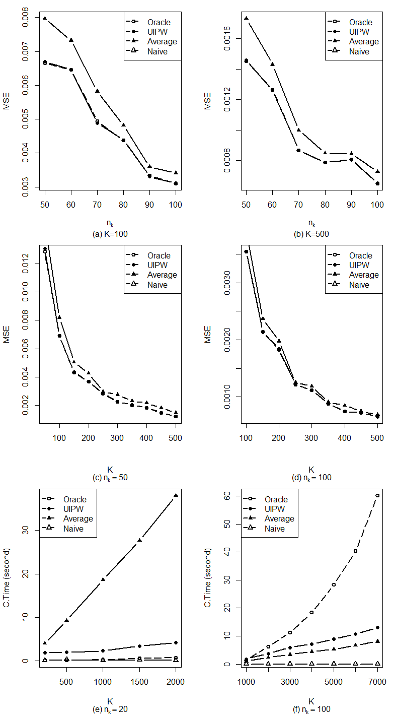
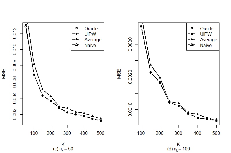
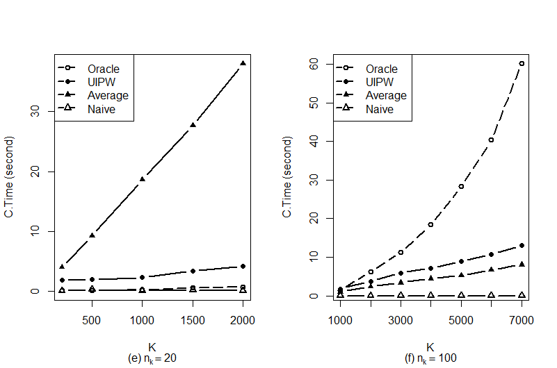
4.1.2 Homoscedastic logistic regression model

We assume $\mathchoice{\hbox{\boldmath$\displaystyle d$}}{\hbox{\boldmath$\textstyle d$}}{\hbox{\boldmath$\scriptstyle d$}}{\hbox{\boldmath$\scriptscriptstyle d$}}_{j}=\{\boldsymbol{\delta}_{j},\mathbf{Y}_{j},\mathbf{X}_{j}\}$, $j=1,\ldots,K$ with $\boldsymbol{\delta}_{j}=(\delta_{1}^{(j)},\ldots,\delta_{n_{j}}^{(j)})^{\top}$ is the indicator vector, $\mathbf{Y}_{j}=(\mathrm{y}_{1}^{(j)},\ldots,\mathrm{y}_{n_{j}}^{(j)})^{\top}$ is a binary response subject to missing at random and $\mathbf{X}_{j}=(\mathrm{x}_{1}^{(j)},\ldots,\mathrm{x}_{n_{j}}^{(j)})^{\top}$ is the covariate vector fully observed, where $\mathrm{y}_{i}^{(j)}\mid\mathrm{x}_{i}^{(j)}$ are independently sampled from a Bernoulli distribution with probability of success $\pi_{j}(\mathbf{X}_{j})=P(\mathbf{Y}_{j}=\mathchoice{\hbox{\boldmath$\displaystyle 1$}}{\hbox{\boldmath$\textstyle 1$}}{\hbox{\boldmath$\scriptstyle 1$}}{\hbox{\boldmath$\scriptscriptstyle 1$}}\mid\mathbf{X}_{j})$. A logistic regression model takes the form:

$$\pi(\mathbf{X}_{j};\boldsymbol{\beta})=\frac{1}{1+e^{-\mathbf{X}_{j}^{\top}\boldsymbol{\beta}}}.$$ (17)

The score function and corresponding negative Hessian matrix for the $j$-th batch of data $\boldsymbol{d}_{j}$ are respectively written as $\mathbf{S}(\boldsymbol{\beta}|\mathchoice{\hbox{\boldmath$\displaystyle d$}}{\hbox{\boldmath$\textstyle d$}}{\hbox{\boldmath$\scriptstyle d$}}{\hbox{\boldmath$\scriptscriptstyle d$}}_{j},\boldsymbol{\alpha})=(1/n_{j})\mathbf{X}_{j}^{\top}\mathbf{D}_{j}(\boldsymbol{\alpha})(\pi_{j}(\mathbf{X}_{j};\boldsymbol{\beta})-\mathbf{Y}_{j})$ and $\mathbf{R}(\boldsymbol{\beta}|\mathchoice{\hbox{\boldmath$\displaystyle d$}}{\hbox{\boldmath$\textstyle d$}}{\hbox{\boldmath$\scriptstyle d$}}{\hbox{\boldmath$\scriptscriptstyle d$}}_{j},\boldsymbol{\alpha})=(1/n_{j})\mathbf{X}_{j}^{\top}\mathbf{Q}_{j}(\boldsymbol{\alpha,\boldsymbol{\beta}})\mathbf{X}_{j}$, where

$$\mathbf{D}_{j}(\boldsymbol{\alpha}) =\mbox{diag}\bigg{(}\frac{\delta_{i}}{\pi(\mathrm{x}_{i}^{(j)};\boldsymbol{\alpha})}\bigg{)},i=1,\ldots,n_{j},$$

$$\mathbf{Q}_{j}(\boldsymbol{\alpha},\boldsymbol{\beta}) =\mbox{diag}\bigg{(}\frac{\delta_{i}}{\pi(\mathrm{x}_{i}^{(j)};\boldsymbol{\alpha})}\pi_{j}(\mathbf{X}_{j};\boldsymbol{\beta})(1-\pi_{j}(\mathbf{X}_{j};\boldsymbol{\beta}))\bigg{)},i=1,\ldots,n_{j}.$$

In this example, when the $j$-th batch of data arrives, we consider the following logistic regression model:

$$\pi(\mathbf{X}_{j};\boldsymbol{\beta}^{0})=\frac{1}{1+exp(-(0.5\mathrm{x}_{i1}^{(j)}+0.5\mathrm{x}_{i2}^{(j)}+\mathrm{x}_{i3}^{(j)}+\mathrm{x}_{i4}^{(j)}))},\quad i\in\mathchoice{\hbox{\boldmath$\displaystyle i$}}{\hbox{\boldmath$\textstyle i$}}{\hbox{\boldmath$\scriptstyle i$}}{\hbox{\boldmath$\scriptscriptstyle i$}}_{j}\cap\mathchoice{\hbox{\boldmath$\displaystyle O$}}{\hbox{\boldmath$\textstyle O$}}{\hbox{\boldmath$\scriptstyle O$}}{\hbox{\boldmath$\scriptscriptstyle O$}},$$ (18)

where $\mathrm{x}_{\cdot t}^{(j)}\sim U(0,1),t=1,2$, $\mathrm{x}_{\cdot t}^{(j)}\sim N(0,1),t=3,4$, and $\boldsymbol{\beta}^{0}=(0.5,0.5,1,1)$. The propensity function is set to be:

$$\pi_{0}(\mathbf{X}_{j};\boldsymbol{\alpha}^{0})=\frac{1}{1+exp(-(0.5\mathrm{x}_{i1}^{(j)}+\mathrm{x}_{i2}^{(j)}+1.5\mathrm{x}_{i3}^{(j)}+0.5\mathrm{x}_{i4}^{(j)}))},\quad i=1,\ldots,n_{j}$$

The simulation results are reported in Table 3 and Figure 2. We have the following findings:

• Mean squared error. Under the criterion of MSE, in Scenario 1, as shown in Table 3, the oracle estimator and our UIPW estimator are more robust to the varing of $K$ than the simple average IPW estimator. In Scenario 2, Figure 2 (a)-(d) implies that the MSE of our UIPW estimator decreases with the increase of $n_{k}$ or $K$, and moreover, our UIPW estimator is significantly superior to the simple average IPW estimator and has similar behavior to the oracle estimator.

• Computation time. Under the criterion of C.Time, the naive estimator takes the least C.Time beacuse it only uses the current data. In Scenario 1, when $N_{k}$ is fixed, Table 3 indicates that when the batch size is as small as $n_{k}=50$, as we said before, the C.Times of the simple average IPW estimator and the naive IPW estimator are larger due to the low convergence rate of the SGD algorithm. In Scenario 2, when $n_{k}$ is small, Figure 2 (e) implies that the simple average estimator takes the most C.Time and our UIPW estimator takes more C.Time than the oracle estimator. However, setting a large $n_{k}$, as shown in Figure 2 (f), the simple average IPW estimator still takes the most C.Time, but the C.Time of the oracle estimator increases rapidly with the increase of $K$, and gradually exceeds that of our UIPW estimator.

Table 3: The MSE and computation time are summarized over 200 replication, under the setting of $N_{K}=100,000$ and $p=4$ for the logistic regression model (17) with batch size $n_{k}$ from 50 to 2000.

	$K=50$, $n_{k}=2000$
	Oracle	UIPW	Average	Naive
MSE	3.39$\times$$10^{-3}$	3.39$\times$$10^{-3}$	5.53$\times$$10^{-3}$	1.20$\times$$10^{-1}$
C.Time(s)	0.39	20.98	24.12	0.47
	$K=100$, $n_{k}=1000$
	Oracle	UIPW	Average	Naive
MSE	3.91$\times$$10^{-3}$	3.89$\times$$10^{-3}$	6.25$\times$$10^{-3}$	4.16$\times$$10^{-1}$
C.Time(s)	0.31	9.43	11.5	0.11
	$K=200$, $n_{k}=500$
	Oracle	UIPW	Average	Naive
MSE	4.33$\times$$10^{-3}$	4.28$\times$$10^{-3}$	1.31$\times$$10^{-2}$	7.65$\times$$10^{-1}$
C.Time(s)	0.73	5.58	7.98	0.03
	$K=500$, $n_{k}=200$
	Oracle	UIPW	Average	Naive
MSE	5.03$\times$$10^{-3}$	4.93$\times$$10^{-3}$	5.14$\times$$10^{-2}$	2.11
C.Time(s)	1.47	3.02	4.88	0.01
	$K=1000$, $n_{k}=100$
	Oracle	UIPW	Average	Naive
MSE	5.22$\times$$10^{-3}$	5.04$\times$$10^{-3}$	1.9$\times$$10^{-1}$	5.52
C.Time(s)	1.61	2.55	5.52	0.01
	$K=2000$, $n_{k}=50$
	Oracle	UIPW	Average	Naive
MSE	1.24$\times$$10^{-2}$	1.27$\times$$10^{-2}$	9.65$\times$$10^{-2}$	3.64
C.Time(s)	3.57	3.83	48.4	0.075

Figure 2: The MSE and computation time in the logistic regression model (17). Note that the MSE of the naive estimator is not depicted in (a), (b), (c) and (d) because it is out of the designed figures.

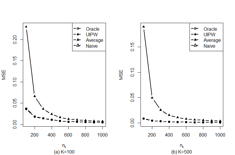
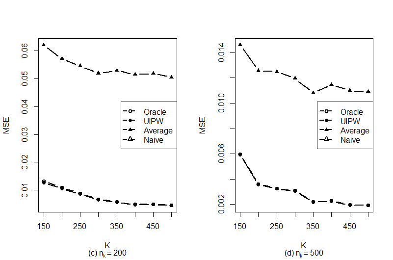
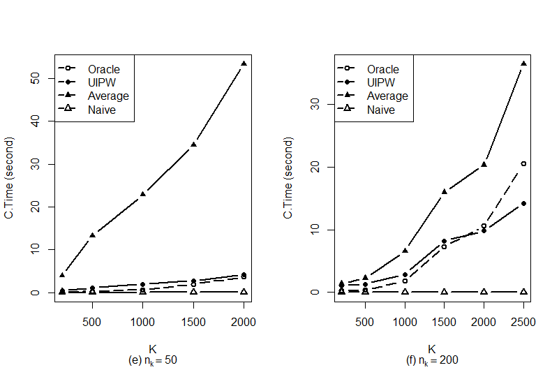
4.1.3 Heteroscedastic logistic regression model

We consider a logistic regression between a binary outcome $\mathbf{Y}$ and an exposure $\mathbf{X}$, controlling for a confounding variable $\mathbf{Z}$. We assume $\mathchoice{\hbox{\boldmath$\displaystyle d$}}{\hbox{\boldmath$\textstyle d$}}{\hbox{\boldmath$\scriptstyle d$}}{\hbox{\boldmath$\scriptscriptstyle d$}}_{j}=\{\boldsymbol{\delta}_{j},\mathbf{Y}_{j},\mathbf{X}_{j},\mathbf{Z}_{j}\}$, $j=1,\ldots,K$ with $\boldsymbol{\delta}_{j}=(\delta_{1}^{(j)},\ldots,\delta_{n_{j}}^{(j)})^{\top}$ is the indicator vector, $\mathbf{Y}_{j}=(\mathrm{y}_{1}^{(j)},\ldots,\mathrm{y}_{n_{j}}^{(j)})^{\top}$ is a binary response subject to missing at random, $\mathbf{X}_{j}=(\mathrm{x}_{1}^{(j)},\ldots,\mathrm{x}_{n_{j}}^{(j)})^{\top}$ and $\mathbf{Z}_{j}=(\mathrm{z}_{1}^{(j)},\ldots,\mathrm{z}_{n_{j}}^{(j)})^{\top}$ are the covariates fully observed, It is assumed that, for the $j$-th batch of data,

$$\text{logit}\{P(\mathbf{Y}_{j}=\boldsymbol{1}\mid\mathbf{X}_{j},\mathbf{Z}_{j})\}=\mathbf{X}_{j}^{\top}\boldsymbol{\beta}+\mathbf{Z}_{j}^{\top}\boldsymbol{\gamma}_{j},$$ (19)

where $\boldsymbol{\gamma}_{j}=(\gamma_{1j},\gamma_{2j})^{\top}$ is the nuisance parameter. We set the true value of $\boldsymbol{\beta}=(0.5,0.5)$. The nuisance parameters $\gamma_{1j}$ and $\gamma_{2j}$ are generated from the uniform distributions $U(-1,1)$ and $U(-2,2)$, respectively. We generate $\mathbf{X}_{j}\sim U(0,1)$ and $\mathbf{Z}_{j}\sim N(\mathbf{X}_{j}-0.3,1)$. The propensity function is set to be:

$$\pi_{0}(\mathbf{X}_{j};\boldsymbol{\alpha}^{0})=\frac{1}{1+\exp(-(0.5\mathrm{x}_{i1}^{(j)}+\mathrm{x}_{i2}^{(j)}))},$$

where $\boldsymbol{\alpha}^{0}=(0.5,1)$. The simulation results are showed in Table 4 and Figure 3. We have the following findings:

• Under the criterion of MSE, in Scenario 1, Table 4 indicates that the MSE of our EUIPW estimator is close to that of the oracle estimator, while the MSE of the simple average IPW estimator is large. In Scenario 2, when $n_{k}$ or $K$ increases, Figure 3 implies that our EUIPW estimator always exhibits similar performances to the oracle estimator. Both of their MSEs tend to decline, but the decline process is not stable.

• Under the criterion of C.Time, as shown in Table 4, the oracle estimator takes the most C.Time because of the computation of the matrix inverse in (13), hence our EUIPW estimator shows clear advantages.

Table 4: The MSE and computation time are summarized over 200 replication, under the setting of $N_{K}=20,000$ and $d=6,p=2,q=2$ for the logistic regression model (19) with batch size $n_{k}$ from 40 to 100.

	$K=40$, $n_{k}=500$
	Oracle	EUIPW	Average	Naive
MSE	3.98$\times$$10^{-3}$	4.16$\times$$10^{-3}$	4.22$\times$$10^{-3}$	1.08$\times$$10^{-1}$
C.Time(s)	129.99	4.31	2.7	0.09
	$K=50$, $n_{k}=400$
	Oracle	EUIPW	Average	Naive
MSE	5.24$\times$$10^{-3}$	5.31$\times$$10^{-3}$	5.72$\times$$10^{-3}$	3.2$\times$$10^{-1}$
C.Time(s)	115.13	3.02	2.92	0.08
	$K=80$, $n_{k}=250$
	Oracle	EUIPW	Average	Naive
MSE	7.11$\times$$10^{-3}$	7.28$\times$$10^{-3}$	8.33$\times$$10^{-3}$	4.6$\times$$10^{-1}$
C.Time(s)	142.86	1.68	1.51	0.05
	$K=100$, $n_{k}=200$
	Oracle	EUIPW	Average	Naive
MSE	8.99$\times$$10^{-3}$	9.08$\times$$10^{-3}$	1.03$\times$$10^{-2}$	1.65
C.Time(s)	117	1.4	1.68	0.08

Figure 3: The MSE in the logistic regression model (19). Note that the MSE of the naive estimator is not depicted in (a) and (b) because it is out of the designed figures.

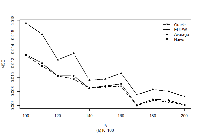
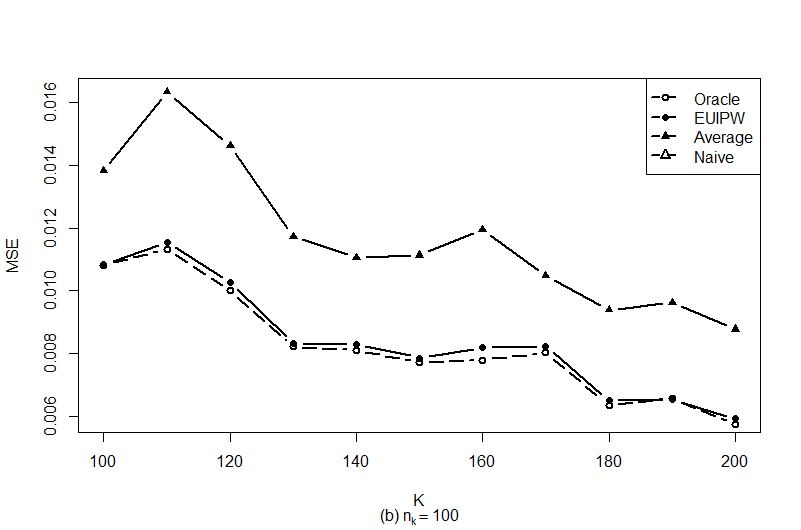
4.2 Real data analysis

We apply the proposed method UIPW to the National Alzheimer’s Coordinating Center (NACC) Uniform Data Set. We choose the age (NACCAGE), diabetes (DIABETES, yes/no), depression or dysphoria (DEPD, yes/no) and Mini-Mental State Exam (NACCMMSE) as covariates according to Chen & Zhou (2011). As introduced by NACC, we determine whether someone has Alzheimer’s disease (AD) based on presumptive etiologic diagnosis of the cognitive disorder (NACCALZD) and cognitive status (NACCUDSD). That is, someone has AD if NACCALZD = 1 and NACCUDSD = 4, otherwise not. Let the response $Y=1$ if someone has AD, otherwise $Y=0$. Our goal is to analyze the relationship between selected covariates and AD.

In this example, the streaming data set were formed by monthly visitor data from the period of 7 years over January 2008 to March 2015, with $K=87$ batches of data and a total simple size $N_{K}=69688$. However, patients may miss a clinic visit or refuse to undergo a clinical examination during the clinic visit, leading to the incomplete responses. According to Chen & Zhou (2011) the MAR mechanism is reasonable. There are 10359 subjects with missing response accounts for 14.8%. Because the response $Y$ is a binary outcome, we utilize (15) and (17) as the regression models. We apply our proposed method to construct updatable sequentially parameter estimates.

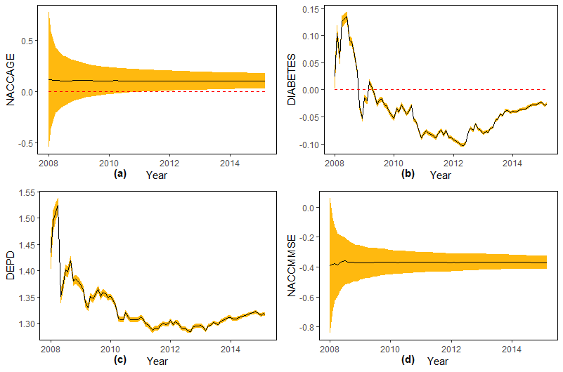
Figure 4: Trace plots for the coefficient estimates and 95% pointwise confidence bands of regression coefficients. Note that the confidence bands in (b) is too narrow to show clearly.

Figure 4 depicts the 95% pointwise confidence bands of all regression coefficients. It is seen that with more batches of data arrived, the confidence bands became narrower. In Figure 4, (a) and (c) show that AD is positively correlated with NACCAGE and DEPD, meaning that older or more depressed or dysphoric people have a higher prevalence. It is interesting to find that the trace plot for the DIABETES shows a downward trend from positive to negative as the sample size increases. This suggests that diabetes now has a positive effect to protect the occurrence of AD. Figure 4 (d) shows that MMSE has a positive effect to protect the occurrence of AD.

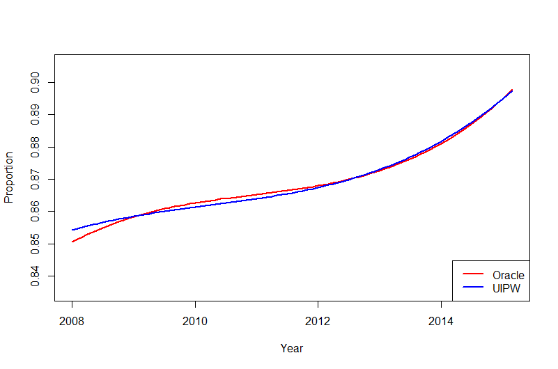
Figure 5: The proportion of correct classifications for the UIPW method and oracle method.

Furthermore, the complete data in the above streaming data set is used to evaluate the UIPW estimator. Figure 5 shows the proportion of correct classifications for the UIPW method and the oracle method when the classification threshold is 0.5. It is seen that the proportion of correct classifications for the UIPW method increases when more data are obtained. To accurately evaluate the performance of the UIPW method and the oracle method as classifiers, we create receiver operating characteristic (ROC) curves using classification probability thresholds between 0 and 1, and then calculate the areas under the ROC curves (AUC). AUC is one of the most important evaluation metrics for measuring the performance of any classification model. It is a performance measurement for a classification problem at various thresholds settings. The larger the value of AUC, the better the effect of classifier. As shown in Table 5, both the AUCs are between 0.85 and 0.95, meaning that both the UIPW method and the oracle method have good performance.

Table 5: The AUCs for the UIPW classifier and the oracle classifier

Method	AUC
UIPW	0.9167
Oracle	0.9173

5 Conclusions and future works

As shown in Introduction, although a large number of statistical methods and computational recipes have been developed to address the challenges of analyzing the models with streaming data sets or missing data separately, the strategy of online updating IPW estimation with missing response in streaming data sets has not been built in the existing literature. To address these issues, we propose the updatable inverse probability weighting (UIPW) estimation via a two-step online updating algorithm in the previous sections. Both the inverse probability weights and the estimator of the parameter of interest can update simultaneously. This is a unified framework because our two-step online updating algorithm can not only deal with the problem concerned in this paper, but also is useful for all models with two types of parameters, one of which is ragarded as the nuisance parameter. Moreover, our UIPW estimator overcomes the memory constraint and is adaptive to the situation where streaming data sets arrive fast and perpetually. Both the proposed statistical methodology and the computational algorithms have been justified theoretically and examined numerically in the setting of GLMs. Summary statistics involved in our proposed method have been verified asymptotically equivalent to the classical sufficient statistic.

In order to extend the UIPW estimation under heterogeneous conditions, motivated by theories of efficient score, the efficient score function is constructed and then the efficient updatable inverse probability weighted (EUIPW) estimation is established. Through the simulation study in Section 4, it is demonstrated that EUIPW estimation is much better than the competitors.

The research can be further improved from the following aspects. Firstly, this paper mainly focused on the parametric model, for the nonparametric model, we will encounter new challenges such as the curse of dimensionality and the bandwidth selection. Secondly, it is natural to think of constructing the updatable imputation method. In the offline framework, most of the imputation methods impute missing response by estimating the conditional expectation of $Y$ given $X$ or conditional density of $Y$ given $X$. However, in the online framework, it is difficult to derive the updatable estimator of the conditional expectation of $Y$ given $X$ or conditional density of $Y$ given $X$ when we don’t store the historical data. Wellenzohn et al. (2017) proposed Top-k Case Matching (TKCM) to impute missing values in streams of time series data. But TKCM defines for each time series a set of reference time series and exploits similar historical situations in the reference time series for the imputation. However, we focus on streaming data sets without any reference streaming data sets. Furthermore, the application of augmented IPW method in streaming data sets can be researched. Thirdly, Taylor et al. (2022) researched the transfer learning when the distributions of $k$-th batch of data and $(k+1)$-th batch of data are the same in some aspects of distribution. This is instructive for us to further study UIPW estimation for the heterogeneous scenario. These are interesting issues and worthy of further investigation in the future.

6 Acknowledgements

The research was supported by the National Key R&D Program of China (grant No. 2018YFA0703900), the National Natural Science Foundation of China (grant No. 11971265) and the National Statistical Science Research Project (grant No. 2022LD03).

Appendix A

A.1. Proof of Theorem 2

Assume that conditions C1-C7 given in Section 2.2 hold. When the $k$-th batch of data arrives, the oracle estimator $\hat{\boldsymbol{\beta}}_{N_{k}}^{*}$ is the solution of

$$\sum_{j=1}^{k}\mathbf{S}(\boldsymbol{\beta}|\mathchoice{\hbox{\boldmath$\displaystyle d$}}{\hbox{\boldmath$\textstyle d$}}{\hbox{\boldmath$\scriptstyle d$}}{\hbox{\boldmath$\scriptscriptstyle d$}}_{j},\boldsymbol{\alpha}_{N_{k}}^{*})=\mathchoice{\hbox{\boldmath$\displaystyle 0$}}{\hbox{\boldmath$\textstyle 0$}}{\hbox{\boldmath$\scriptstyle 0$}}{\hbox{\boldmath$\scriptscriptstyle 0$}},$$

where $\boldsymbol{\alpha}_{N_{k}}^{*}=\underset{\boldsymbol{\alpha}\in\mathbb{R}^{p}}{\arg\max}\sum_{j=1}^{k}\sum_{i\in\mathchoice{\hbox{\boldmath$\displaystyle i$}}{\hbox{\boldmath$\textstyle i$}}{\hbox{\boldmath$\scriptstyle i$}}{\hbox{\boldmath$\scriptscriptstyle i$}}_{j}}\log\bigg{\{}\pi(X_{i};\boldsymbol{\alpha})^{\delta_{i}}\big{[}1-\pi(X_{i};\boldsymbol{\alpha})\big{]}^{(1-\delta_{i})}\bigg{\}}$.

Let $\boldsymbol{\beta}^{0}$ be the true value of the parameter $\boldsymbol{\beta}$ and $\hat{\boldsymbol{\beta}}_{k}$ be the updatable estimator. For the first batch of data $\mathchoice{\hbox{\boldmath$\displaystyle d$}}{\hbox{\boldmath$\textstyle d$}}{\hbox{\boldmath$\scriptstyle d$}}{\hbox{\boldmath$\scriptscriptstyle d$}}_{1}$, we have $\hat{\boldsymbol{\beta}}_{1}=\hat{\boldsymbol{\beta}}_{N_{1}}^{*}$. Next we prove the consistency of $\hat{\boldsymbol{\beta}}_{k}$ when $k\geq 2$ by the method of induction.

Define a function

$$\begin{split}g_{k}(\boldsymbol{\beta})=\frac{1}{N_{k}}\sum_{j=1}^{k-1}\mathbf{L}_{1}(\hat{\boldsymbol{\beta}}_{j}|\mathchoice{\hbox{\boldmath$\displaystyle d$}}{\hbox{\boldmath$\textstyle d$}}{\hbox{\boldmath$\scriptstyle d$}}{\hbox{\boldmath$\scriptscriptstyle d$}}_{j},\hat{\boldsymbol{\alpha}}_{j})(\hat{\boldsymbol{\alpha}}_{k}-\hat{\boldsymbol{\alpha}}_{k-1})+\frac{1}{N_{k}}\sum_{j=1}^{k-1}\mathbf{L}_{2}(\hat{\boldsymbol{\beta}}_{j}|\mathchoice{\hbox{\boldmath$\displaystyle d$}}{\hbox{\boldmath$\textstyle d$}}{\hbox{\boldmath$\scriptstyle d$}}{\hbox{\boldmath$\scriptscriptstyle d$}}_{j},\hat{\boldsymbol{\alpha}}_{j})(\boldsymbol{\beta}-\hat{\boldsymbol{\beta}}_{k-1})\\ +\frac{1}{N_{k}}\mathbf{S}(\boldsymbol{\beta}|\mathchoice{\hbox{\boldmath$\displaystyle d$}}{\hbox{\boldmath$\textstyle d$}}{\hbox{\boldmath$\scriptstyle d$}}{\hbox{\boldmath$\scriptscriptstyle d$}}_{k},\hat{\boldsymbol{\alpha}}_{k}).\end{split}$$ (20)

According to equation (7), the updatable estimator $\hat{\boldsymbol{\beta}}_{k}$ satisfies

$$g_{k}(\hat{\boldsymbol{\beta}}_{k})=0.$$ (21)

When $\hat{\boldsymbol{\beta}}_{k-1}$ is consistent, we have

$$\begin{split}g_{k}(\boldsymbol{\beta}^{0})=\frac{1}{N_{k}}\sum_{j=1}^{k-1}\mathbf{L}_{1}(\hat{\boldsymbol{\beta}}_{j}|\mathchoice{\hbox{\boldmath$\displaystyle d$}}{\hbox{\boldmath$\textstyle d$}}{\hbox{\boldmath$\scriptstyle d$}}{\hbox{\boldmath$\scriptscriptstyle d$}}_{j},\hat{\boldsymbol{\alpha}}_{j})(\hat{\boldsymbol{\alpha}}_{k}-\hat{\boldsymbol{\alpha}}_{k-1})+\frac{1}{N_{k}}\sum_{j=1}^{k-1}\mathbf{L}_{2}(\hat{\boldsymbol{\beta}}_{j}|\mathchoice{\hbox{\boldmath$\displaystyle d$}}{\hbox{\boldmath$\textstyle d$}}{\hbox{\boldmath$\scriptstyle d$}}{\hbox{\boldmath$\scriptscriptstyle d$}}_{j},\hat{\boldsymbol{\alpha}}_{j})(\boldsymbol{\beta}^{0}-\hat{\boldsymbol{\beta}}_{k-1})\\ +\frac{1}{N_{k}}\mathbf{S}(\boldsymbol{\beta}^{0}|\mathchoice{\hbox{\boldmath$\displaystyle d$}}{\hbox{\boldmath$\textstyle d$}}{\hbox{\boldmath$\scriptstyle d$}}{\hbox{\boldmath$\scriptscriptstyle d$}}_{k},\hat{\boldsymbol{\alpha}}_{k})=o_{p}(1).\end{split}$$ (22)

Taking the difference between equations (22) and (21), we attain

$$\begin{split}g_{k}(\boldsymbol{\beta}^{0})-g_{k}(\hat{\boldsymbol{\beta}}_{k})=\frac{1}{N_{k}}\sum_{j=1}^{k-1}\mathbf{L}_{2}(\hat{\boldsymbol{\beta}}_{j}|\mathchoice{\hbox{\boldmath$\displaystyle d$}}{\hbox{\boldmath$\textstyle d$}}{\hbox{\boldmath$\scriptstyle d$}}{\hbox{\boldmath$\scriptscriptstyle d$}}_{j},\hat{\boldsymbol{\alpha}}_{j})(\boldsymbol{\beta}^{0}-\hat{\boldsymbol{\beta}}_{k})-\frac{1}{N_{k}}\mathbf{S}(\hat{\boldsymbol{\beta}}_{k}|\mathchoice{\hbox{\boldmath$\displaystyle d$}}{\hbox{\boldmath$\textstyle d$}}{\hbox{\boldmath$\scriptstyle d$}}{\hbox{\boldmath$\scriptscriptstyle d$}}_{k},\hat{\boldsymbol{\alpha}}_{k})\\ +\frac{1}{N_{k}}\mathbf{S}(\boldsymbol{\beta}^{0}|\mathchoice{\hbox{\boldmath$\displaystyle d$}}{\hbox{\boldmath$\textstyle d$}}{\hbox{\boldmath$\scriptstyle d$}}{\hbox{\boldmath$\scriptscriptstyle d$}}_{k},\hat{\boldsymbol{\alpha}}_{k})=o_{p}(1).\end{split}$$ (23)

Taking the first-order Taylor series expansion of $\mathbf{S}(\hat{\boldsymbol{\beta}}_{k}|\mathchoice{\hbox{\boldmath$\displaystyle d$}}{\hbox{\boldmath$\textstyle d$}}{\hbox{\boldmath$\scriptstyle d$}}{\hbox{\boldmath$\scriptscriptstyle d$}}_{k},\hat{\boldsymbol{\alpha}}_{k})$ in equation (23) around $\boldsymbol{\beta}^{0}$, we have

$$\begin{split}\mathbf{S}(\hat{\boldsymbol{\beta}}_{k}|\mathchoice{\hbox{\boldmath$\displaystyle d$}}{\hbox{\boldmath$\textstyle d$}}{\hbox{\boldmath$\scriptstyle d$}}{\hbox{\boldmath$\scriptscriptstyle d$}}_{k},\hat{\boldsymbol{\alpha}}_{k})=\mathbf{S}(\boldsymbol{\beta}^{0}|\mathchoice{\hbox{\boldmath$\displaystyle d$}}{\hbox{\boldmath$\textstyle d$}}{\hbox{\boldmath$\scriptstyle d$}}{\hbox{\boldmath$\scriptscriptstyle d$}}_{k},\hat{\boldsymbol{\alpha}}_{k})+\bigg{[}\mathbf{R}_{\boldsymbol{\beta}}(\boldsymbol{\beta}^{0}|\mathchoice{\hbox{\boldmath$\displaystyle d$}}{\hbox{\boldmath$\textstyle d$}}{\hbox{\boldmath$\scriptstyle d$}}{\hbox{\boldmath$\scriptscriptstyle d$}}_{k},\hat{\boldsymbol{\alpha}}_{k})-\mathbf{R}_{\boldsymbol{\beta}}(\boldsymbol{\beta}^{0}|\mathchoice{\hbox{\boldmath$\displaystyle d$}}{\hbox{\boldmath$\textstyle d$}}{\hbox{\boldmath$\scriptstyle d$}}{\hbox{\boldmath$\scriptscriptstyle d$}}_{k},\hat{\boldsymbol{\alpha}}_{k})\\ +\mathbf{R}_{\boldsymbol{\beta}}(\boldsymbol{\phi}_{k}|\mathchoice{\hbox{\boldmath$\displaystyle d$}}{\hbox{\boldmath$\textstyle d$}}{\hbox{\boldmath$\scriptstyle d$}}{\hbox{\boldmath$\scriptscriptstyle d$}}_{k},\hat{\boldsymbol{\alpha}}_{k})\bigg{]}(\hat{\boldsymbol{\beta}}_{k}-\boldsymbol{\beta}^{0}),\end{split}$$ (24)

where $\boldsymbol{\phi}_{k}$ lies in between $\hat{\boldsymbol{\beta}}_{k}$ and $\boldsymbol{\beta}^{0}$. By the Lipschitz continuity in condition C7, there exists $\boldsymbol{C}(\boldsymbol{d}_{k})\textgreater 0$ such that

$$\parallel\mathbf{R}_{\boldsymbol{\beta}}(\boldsymbol{\phi}_{k}|\boldsymbol{d}_{k},\hat{\boldsymbol{\alpha}}_{k},)-\mathbf{R}_{\boldsymbol{\beta}}(\boldsymbol{\beta}^{0}|\boldsymbol{d}_{k},\hat{\boldsymbol{\alpha}}_{k},)\parallel\leq\boldsymbol{C}(\boldsymbol{d}_{k})\parallel\boldsymbol{\phi}_{k}-\boldsymbol{\beta}^{0}\parallel\leq\boldsymbol{C}(\boldsymbol{d}_{k})\parallel\hat{\boldsymbol{\beta}}_{k}-\boldsymbol{\beta}^{0}\parallel.$$ (25)

Then we can rewrite equation (24) as

$$\mathbf{S}(\hat{\boldsymbol{\beta}}_{k}|\mathchoice{\hbox{\boldmath$\displaystyle d$}}{\hbox{\boldmath$\textstyle d$}}{\hbox{\boldmath$\scriptstyle d$}}{\hbox{\boldmath$\scriptscriptstyle d$}}_{k},\hat{\boldsymbol{\alpha}}_{k})=\mathbf{S}(\boldsymbol{\beta}^{0}|\mathchoice{\hbox{\boldmath$\displaystyle d$}}{\hbox{\boldmath$\textstyle d$}}{\hbox{\boldmath$\scriptstyle d$}}{\hbox{\boldmath$\scriptscriptstyle d$}}_{k},\hat{\boldsymbol{\alpha}}_{k})+\mathbf{R}_{\boldsymbol{\beta}}(\boldsymbol{\beta}^{0}|\mathchoice{\hbox{\boldmath$\displaystyle d$}}{\hbox{\boldmath$\textstyle d$}}{\hbox{\boldmath$\scriptstyle d$}}{\hbox{\boldmath$\scriptscriptstyle d$}}_{k},\hat{\boldsymbol{\alpha}}_{k})(\hat{\boldsymbol{\beta}}_{k}-\boldsymbol{\beta}^{0})+O_{p}(n_{k}\parallel\hat{\boldsymbol{\beta}}_{k}-\boldsymbol{\beta}^{0}\parallel^{2}).$$ (26)

Combining equations (23) and (26) yields

$$\begin{split}g_{k}(\boldsymbol{\beta}^{0})-g_{k}(\hat{\boldsymbol{\beta}}_{k})=\frac{1}{N_{k}}\bigg{[}\sum_{j=1}^{k-1}\mathbf{L}_{2}(\hat{\boldsymbol{\beta}}_{j}|\mathchoice{\hbox{\boldmath$\displaystyle d$}}{\hbox{\boldmath$\textstyle d$}}{\hbox{\boldmath$\scriptstyle d$}}{\hbox{\boldmath$\scriptscriptstyle d$}}_{j},\hat{\boldsymbol{\alpha}}_{j})+\mathbf{R}_{\boldsymbol{\beta}}(\boldsymbol{\beta}^{0}|\mathchoice{\hbox{\boldmath$\displaystyle d$}}{\hbox{\boldmath$\textstyle d$}}{\hbox{\boldmath$\scriptstyle d$}}{\hbox{\boldmath$\scriptscriptstyle d$}}_{k},\hat{\boldsymbol{\alpha}}_{k})\bigg{]}(\hat{\boldsymbol{\beta}}_{0}-\hat{\boldsymbol{\beta}}_{k})\\ +O_{p}(\frac{n_{k}}{N_{k}}\parallel\hat{\boldsymbol{\beta}}_{k}-\boldsymbol{\beta}^{0}\parallel^{2})=o_{p}(1).\end{split}$$ (27)

We know that $\hat{\boldsymbol{\alpha}}_{j}$ is consistent for $j=1,\ldots,k$. Therefore, by conditions C5, $\frac{1}{N_{k}}[\sum_{j=1}^{k-1}\mathbf{L}_{2}(\hat{\boldsymbol{\beta}}_{j}|\mathchoice{\hbox{\boldmath$\displaystyle d$}}{\hbox{\boldmath$\textstyle d$}}{\hbox{\boldmath$\scriptstyle d$}}{\hbox{\boldmath$\scriptscriptstyle d$}}_{j},\hat{\boldsymbol{\alpha}}_{j})+\mathbf{R}_{\boldsymbol{\beta}}(\boldsymbol{\beta}^{0}|\mathchoice{\hbox{\boldmath$\displaystyle d$}}{\hbox{\boldmath$\textstyle d$}}{\hbox{\boldmath$\scriptstyle d$}}{\hbox{\boldmath$\scriptscriptstyle d$}}_{k},\hat{\boldsymbol{\alpha}}_{k})]$ is positive definite. Under the assumption $\hat{\boldsymbol{\beta}}_{j}$ is consistent for $j=1,\ldots,k-1$. It follows that $\hat{\boldsymbol{\beta}}_{k}-\boldsymbol{\beta}^{0}\overset{P}{\rightarrow}0$, as $N_{k}\rightarrow\infty$.

A.2. Proof of Theorem 3

(a) When $k=1$, that is, for the first batch of data $\mathchoice{\hbox{\boldmath$\displaystyle d$}}{\hbox{\boldmath$\textstyle d$}}{\hbox{\boldmath$\scriptstyle d$}}{\hbox{\boldmath$\scriptscriptstyle d$}}_{1}$, $n_{1}=N_{1}$, the oracle estimator $\hat{\boldsymbol{\beta}}_{N_{1}}^{*}=\hat{\boldsymbol{\beta}}_{1}$ satisfies $(1/N_{1})\mathbf{S}(\hat{\boldsymbol{\beta}}_{1}|\boldsymbol{d}_{1},\hat{\boldsymbol{\alpha}}_{1})=0$ and $\sqrt{N_{1}}(\hat{\boldsymbol{\beta}}_{1}-\boldsymbol{\beta}^{0})\overset{d}{\rightarrow}N(0,\boldsymbol{\Sigma}^{0})$, as $N_{1}=n_{1}\rightarrow\infty$. Taking the first-order Taylor series expansion of $\mathbf{S}(\boldsymbol{\beta}^{0}|\mathchoice{\hbox{\boldmath$\displaystyle d$}}{\hbox{\boldmath$\textstyle d$}}{\hbox{\boldmath$\scriptstyle d$}}{\hbox{\boldmath$\scriptscriptstyle d$}}_{1},\hat{\boldsymbol{\alpha}}_{1})$ around $\hat{\boldsymbol{\beta}}_{1}$, we have

$$\frac{1}{N_{1}}\mathbf{S}(\boldsymbol{\beta}^{0}|\boldsymbol{d}_{1},\hat{\boldsymbol{\alpha}}_{1})=\frac{1}{N_{1}}\mathbf{R}_{\boldsymbol{\beta}}(\hat{\boldsymbol{\beta}}_{1}|\boldsymbol{d}_{1},\hat{\boldsymbol{\alpha}}_{1})(\boldsymbol{\beta}^{0}-\hat{\boldsymbol{\beta}}_{1})+O_{p}(\frac{n_{1}}{N_{1}}\parallel\hat{\boldsymbol{\beta}}_{1}-\boldsymbol{\beta}^{0}\parallel^{2}).$$ (28)

(b)When $k\geq 2$, considering updating $\hat{\boldsymbol{\beta}}_{k-1}$ to $\hat{\boldsymbol{\beta}}_{k}$. The oracle estimator $\hat{\boldsymbol{\beta}}_{N_{k}}^{*}$ satisfies $(1/N_{k})\sum_{j=1}^{k}\mathbf{S}(\hat{\boldsymbol{\beta}}_{N_{k}}^{*}|\boldsymbol{d}_{j},\hat{\boldsymbol{\alpha}}_{N_{k}}^{*})=0$. According to (26)

$$\begin{split}\frac{1}{N_{k}}\sum_{j=1}^{k}\mathbf{S}(\boldsymbol{\beta}^{0}|\boldsymbol{d}_{j},\hat{\boldsymbol{\alpha}}_{N_{k}}^{*})+\frac{1}{N_{k}}\sum_{j=1}^{k}\mathbf{R}_{\boldsymbol{\beta}}(\boldsymbol{\beta}^{0}|\boldsymbol{d}_{j},\hat{\boldsymbol{\alpha}}_{N_{k}}^{*})(\hat{\boldsymbol{\beta}}_{N_{k}}^{*}-\boldsymbol{\beta}^{0})\\ +O_{p}(\parallel\hat{\boldsymbol{\beta}}_{N_{k}}^{*}-\boldsymbol{\beta}^{0}\parallel^{2})=\boldsymbol{0}.\end{split}$$ (29)

According to equations (20), (21) and (27), we know that

$$g_{k}(\boldsymbol{\beta}^{0})= \frac{1}{N_{k}}\sum_{j=1}^{k-1}\mathbf{L}_{1}(\hat{\boldsymbol{\beta}}_{j}|\mathchoice{\hbox{\boldmath$\displaystyle d$}}{\hbox{\boldmath$\textstyle d$}}{\hbox{\boldmath$\scriptstyle d$}}{\hbox{\boldmath$\scriptscriptstyle d$}}_{j},\hat{\boldsymbol{\alpha}}_{j})(\hat{\boldsymbol{\alpha}}_{k}-\hat{\boldsymbol{\alpha}}_{k-1})+\frac{1}{N_{k}}\sum_{j=1}^{k-1}\mathbf{L}_{2}(\hat{\boldsymbol{\beta}}_{j}|\mathchoice{\hbox{\boldmath$\displaystyle d$}}{\hbox{\boldmath$\textstyle d$}}{\hbox{\boldmath$\scriptstyle d$}}{\hbox{\boldmath$\scriptscriptstyle d$}}_{j},\hat{\boldsymbol{\alpha}}_{j})(\boldsymbol{\beta}^{0}-\hat{\boldsymbol{\beta}}_{k-1})$$

$$+\frac{1}{N_{k}}\mathbf{S}(\boldsymbol{\beta}^{0}|\mathchoice{\hbox{\boldmath$\displaystyle d$}}{\hbox{\boldmath$\textstyle d$}}{\hbox{\boldmath$\scriptstyle d$}}{\hbox{\boldmath$\scriptscriptstyle d$}}_{k},\hat{\boldsymbol{\alpha}}_{k})$$

$$= \frac{1}{N_{k}}\bigg{[}\sum_{j=1}^{k-1}\mathbf{L}_{2}(\hat{\boldsymbol{\beta}}_{j}|\mathchoice{\hbox{\boldmath$\displaystyle d$}}{\hbox{\boldmath$\textstyle d$}}{\hbox{\boldmath$\scriptstyle d$}}{\hbox{\boldmath$\scriptscriptstyle d$}}_{j},\hat{\boldsymbol{\alpha}}_{j})+\mathbf{R}_{\boldsymbol{\beta}}(\boldsymbol{\beta}^{0}|\mathchoice{\hbox{\boldmath$\displaystyle d$}}{\hbox{\boldmath$\textstyle d$}}{\hbox{\boldmath$\scriptstyle d$}}{\hbox{\boldmath$\scriptscriptstyle d$}}_{k},\hat{\boldsymbol{\alpha}}_{k})\bigg{]}(\hat{\boldsymbol{\beta}}_{0}-\hat{\boldsymbol{\beta}}_{k})$$

$$+O_{p}(\frac{n_{k}}{N_{k}}\parallel\hat{\boldsymbol{\beta}}_{k}-\boldsymbol{\beta}^{0}\parallel^{2})=o_{p}(1).$$

It follows that

$$\begin{split}&\frac{1}{N_{k}}\bigg{[}\sum_{j=1}^{k-1}\mathbf{L}_{2}(\hat{\boldsymbol{\beta}}_{j}|\mathchoice{\hbox{\boldmath$\displaystyle d$}}{\hbox{\boldmath$\textstyle d$}}{\hbox{\boldmath$\scriptstyle d$}}{\hbox{\boldmath$\scriptscriptstyle d$}}_{j},\hat{\boldsymbol{\alpha}}_{j})+\mathbf{R}_{\boldsymbol{\beta}}(\boldsymbol{\beta}^{0}|\mathchoice{\hbox{\boldmath$\displaystyle d$}}{\hbox{\boldmath$\textstyle d$}}{\hbox{\boldmath$\scriptstyle d$}}{\hbox{\boldmath$\scriptscriptstyle d$}}_{k},\hat{\boldsymbol{\alpha}}_{k})\bigg{]}(\hat{\boldsymbol{\beta}}_{k}-\boldsymbol{\beta}^{0})+\frac{1}{N_{k}}\sum_{j=1}^{k-1}\mathbf{L}_{2}(\hat{\boldsymbol{\beta}}_{j}|\mathchoice{\hbox{\boldmath$\displaystyle d$}}{\hbox{\boldmath$\textstyle d$}}{\hbox{\boldmath$\scriptstyle d$}}{\hbox{\boldmath$\scriptscriptstyle d$}}_{j},\hat{\boldsymbol{\alpha}}_{j})\\ &\times(\boldsymbol{\beta}^{0}-\hat{\boldsymbol{\beta}}_{k-1})+\frac{1}{N_{k}}\mathbf{S}(\boldsymbol{\beta}^{0}|\mathchoice{\hbox{\boldmath$\displaystyle d$}}{\hbox{\boldmath$\textstyle d$}}{\hbox{\boldmath$\scriptstyle d$}}{\hbox{\boldmath$\scriptscriptstyle d$}}_{k},\hat{\boldsymbol{\alpha}}_{k})+O_{p}(\frac{n_{k}}{N_{k}}\parallel\hat{\boldsymbol{\beta}}_{k}-\boldsymbol{\beta}^{0}\parallel^{2})+o_{p}(1)=\mathchoice{\hbox{\boldmath$\displaystyle 0$}}{\hbox{\boldmath$\textstyle 0$}}{\hbox{\boldmath$\scriptstyle 0$}}{\hbox{\boldmath$\scriptscriptstyle 0$}}.\end{split}$$ (30)

Similarly to equation (28), at the $(k-1)$-th batch of data, it is easy to show that

$$\begin{split}\frac{1}{N_{k-1}}\sum_{j=1}^{k-1}\mathbf{S}(\boldsymbol{\beta}^{0}|\boldsymbol{d}_{j},\hat{\boldsymbol{\alpha}}_{k-1})&=\frac{1}{N_{k-1}}\sum_{j=1}^{k-1}\mathbf{S}(\boldsymbol{\beta}^{0}|\boldsymbol{d}_{j},\hat{\boldsymbol{\alpha}}_{k})+o_{p}(1)\\ &=\frac{1}{N_{k-1}}\sum_{j=1}^{k-1}\mathbf{L}_{2}(\hat{\boldsymbol{\beta}}_{j}|\boldsymbol{d}_{j},\hat{\boldsymbol{\alpha}}_{j})(\boldsymbol{\beta}^{0}-\hat{\boldsymbol{\beta}}_{k-1})\\ &+O_{p}(\sum_{j=1}^{k-1}\frac{n_{j}}{N_{k-1}}\parallel\hat{\boldsymbol{\beta}}_{j}-\boldsymbol{\beta}^{0}\parallel^{2})+o_{p}(1).\end{split}$$ (31)

Plugging equation (31) into equation (30), we obtain

$$\begin{split}&\frac{1}{N_{k}}\sum_{j=1}^{k}\mathbf{S}(\boldsymbol{\beta}^{0}|\boldsymbol{d}_{j},\hat{\boldsymbol{\alpha}}_{k})+\frac{1}{N_{k}}\bigg{\{}\sum_{j=1}^{k-1}\mathbf{L}_{2}(\hat{\boldsymbol{\beta}}_{j}|\boldsymbol{d}_{j},\hat{\boldsymbol{\alpha}}_{j})+\mathbf{R}_{\boldsymbol{\beta}}(\boldsymbol{\beta}^{0}|\boldsymbol{d}_{k},\hat{\boldsymbol{\alpha}}_{k})\bigg{\}}(\hat{\boldsymbol{\beta}}_{k}-\boldsymbol{\beta}^{0})\\ &+\frac{1}{N_{k}}\sum_{j=1}^{k-1}\mathbf{L}_{1}(\hat{\boldsymbol{\beta}}_{j}|\mathchoice{\hbox{\boldmath$\displaystyle d$}}{\hbox{\boldmath$\textstyle d$}}{\hbox{\boldmath$\scriptstyle d$}}{\hbox{\boldmath$\scriptscriptstyle d$}}_{j},\hat{\boldsymbol{\alpha}}_{j})(\hat{\boldsymbol{\alpha}}_{k}-\hat{\boldsymbol{\alpha}}_{k-1})+O_{p}(\sum_{j=1}^{k}\frac{n_{j}}{N_{k}}\parallel\hat{\boldsymbol{\beta}}_{j}-\boldsymbol{\beta}^{0}\parallel^{2})=\boldsymbol{0}.\end{split}$$ (32)

According to Lemma 1 and Theorem 2, $\hat{\boldsymbol{\alpha}}_{j}$ are consistent for $j=1,\ldots,k$ and $\hat{\boldsymbol{\beta}}_{j}$ are consistent for $j=1,\ldots,k-1$. Then, by condition C7, the continuous mapping theorem implies that

$$\begin{split}\frac{1}{N_{k}}\sum_{j=1}^{k}\mathbf{S}(\boldsymbol{\beta}^{0}|\boldsymbol{d}_{j},\hat{\boldsymbol{\alpha}}_{k})+\frac{1}{N_{k}}\sum_{j=1}^{k}\mathbf{R}_{\boldsymbol{\beta}}(\boldsymbol{\beta}^{0}|\boldsymbol{d}_{j},\hat{\boldsymbol{\alpha}}_{j})(\hat{\boldsymbol{\beta}}_{k}-\boldsymbol{\beta}^{0})\\ +O_{p}(\sum_{j=1}^{k}\frac{n_{j}}{N_{k}}\parallel\hat{\boldsymbol{\beta}}_{j}-\boldsymbol{\beta}^{0}\parallel^{2})=\boldsymbol{0}.\end{split}$$ (33)

By condition C5, $\mathcal{I}^{-1}_{N_{k}}(\boldsymbol{\beta}^{0})$ exists, and thus the central limit theorem implies that

$$\sqrt{N_{k}}(\hat{\boldsymbol{\beta}}_{k}-\boldsymbol{\beta}^{0})=\{-\frac{1}{N_{k}}\sum_{j=1}^{k}\mathbf{R}_{\boldsymbol{\beta}}(\boldsymbol{\beta}^{0}|\boldsymbol{d}_{j},\hat{\boldsymbol{\alpha}}_{j})\}^{-1}\frac{1}{\sqrt{N_{k}}}\sum_{j=1}^{k}\mathbf{S}(\boldsymbol{\beta}^{0}|\boldsymbol{d}_{j},\hat{\boldsymbol{\alpha}}_{k})+o_{p}(1).$$ (34)

Taking the first-order Taylor series expansion of $\mathbf{S}(\boldsymbol{\beta}^{0}|\boldsymbol{d}_{j},\hat{\boldsymbol{\alpha}}_{k})$ around $\boldsymbol{\alpha}^{0}$ in (34), we obtain

$$\begin{split}\sqrt{N_{k}}(\hat{\boldsymbol{\beta}}_{k}-\boldsymbol{\beta}^{0})=\bigg{\{}-\frac{1}{N_{k}}\sum_{j=1}^{k}\mathbf{R}_{\boldsymbol{\beta}}(\boldsymbol{\beta}^{0}|\boldsymbol{d}_{j},\hat{\boldsymbol{\alpha}}_{j})\bigg{\}}^{-1}\bigg{\{}\frac{1}{\sqrt{N_{k}}}\sum_{j=1}^{k}\mathbf{S}(\boldsymbol{\beta}^{0}|\boldsymbol{d}_{j},\boldsymbol{\alpha}^{0})\\ +\big{[}\frac{1}{N_{k}}\sum_{j=1}^{k}\mathbf{R}_{\boldsymbol{\alpha}}(\boldsymbol{\beta}^{0}|\boldsymbol{d}_{j},\boldsymbol{\psi}_{k})\sqrt{N_{k}}(\hat{\boldsymbol{\alpha}}_{k}-\boldsymbol{\alpha}^{0})\big{]}\bigg{\}}+o_{p}(1).\end{split}$$ (35)

where $\boldsymbol{\psi}_{k}$ lies in between $\hat{\boldsymbol{\alpha}}_{k}$ and $\boldsymbol{\alpha}^{0}$. According to the asymptotic normality of $\hat{\boldsymbol{\alpha}}_{k}$, we can get

$$\sqrt{N_{k}}(\hat{\boldsymbol{\alpha}}_{k}-\boldsymbol{\alpha}^{0})=\frac{1}{\sqrt{N_{k}}}\sum_{j=1}^{k}\bigg{\{}E\big{[}V(\delta;X,\boldsymbol{\alpha}^{0})V(\delta;X,\boldsymbol{\alpha}^{0})^{\top}\big{]}\bigg{\}}^{-1}\mathbf{V}(\boldsymbol{\delta}_{j};\mathbf{X}_{j},\boldsymbol{\alpha}^{0})+o_{p}(1)$$ (36)

Substituting (36) into (35) gives

$$\begin{split}&\sqrt{N_{k}}(\hat{\boldsymbol{\beta}}_{k}-\boldsymbol{\beta}_{0})=\bigg{\{}-\frac{1}{N_{k}}\sum_{j=1}^{k}\mathbf{R}_{\boldsymbol{\beta}}(\boldsymbol{\beta}^{0}|\boldsymbol{d}_{j},\hat{\boldsymbol{\alpha}}_{j})\bigg{\}}^{-1}\frac{1}{\sqrt{N_{k}}}\sum_{j=1}^{k}\bigg{\{}\mathbf{S}(\boldsymbol{\beta}^{0}|\boldsymbol{d}_{j},\boldsymbol{\alpha}^{0})\\ &+E\big{[}R_{\boldsymbol{\alpha}}(\boldsymbol{\beta}^{0}|W,\boldsymbol{\alpha}^{0})\big{]}\bigg{\{}E\big{[}V(\delta;X,\boldsymbol{\alpha}^{0})V(\delta;X,\boldsymbol{\alpha}^{0})^{\top}\big{]}\bigg{\}}^{-1}\mathbf{V}(\boldsymbol{\delta}_{j};\mathbf{X}_{j},\boldsymbol{\alpha}^{0})\bigg{\}}+o_{p}(1),\end{split}$$ (37)

where $R_{\boldsymbol{\alpha}}(\boldsymbol{\beta}^{0}|W,\boldsymbol{\alpha}^{0})$ is the derivative of $S(\boldsymbol{\beta}^{0}|W,\boldsymbol{\alpha}^{0})$ with respect to $\boldsymbol{\alpha}$. In addition, for the observed data $W$, we have

$$E\big{[}S(\boldsymbol{\beta}|W,\boldsymbol{\alpha})\big{]}=\int S(\boldsymbol{\beta}|W,\boldsymbol{\alpha})p(W;\boldsymbol{\beta},\boldsymbol{\alpha})dW=0,$$ (38)

where $p(W;\boldsymbol{\beta},\boldsymbol{\alpha})$ is the joint distribution function. Taking the derivative of equation (38)

$$\begin{split}\frac{\partial}{\partial\boldsymbol{\alpha}}E[S(\boldsymbol{\beta}|W,\boldsymbol{\alpha})]&=\int\frac{\partial}{\partial\boldsymbol{\alpha}}S(\boldsymbol{\beta}|W,\boldsymbol{\alpha})p(W;\boldsymbol{\beta},\boldsymbol{\alpha})dW+\int S(\boldsymbol{\beta}|W,\boldsymbol{\alpha})\frac{\partial}{\partial\boldsymbol{\alpha}}p(W;\boldsymbol{\beta},\boldsymbol{\alpha})dW\\ &=E[R_{\boldsymbol{\alpha}}(\boldsymbol{\beta}|W,\boldsymbol{\alpha})]+\int S(\boldsymbol{\beta}|W,\boldsymbol{\alpha})\frac{\frac{\partial}{\partial\boldsymbol{\alpha}}p(W;\boldsymbol{\beta},\boldsymbol{\alpha})}{p(W;\boldsymbol{\beta},\boldsymbol{\alpha})}p(W;\boldsymbol{\beta},\boldsymbol{\alpha})dW\\ &=E[R_{\boldsymbol{\alpha}}(\boldsymbol{\beta}|W,\boldsymbol{\alpha})]+E[S(\boldsymbol{\beta}|W,\boldsymbol{\alpha})V(\delta;X,\boldsymbol{\alpha})]=0.\end{split}$$ (39)

By the weak law of large numbers and the consistency of $\hat{\boldsymbol{\alpha}}_{j}$ for $j=1,\ldots,k$, we have $(1/N_{k})\sum_{j=1}^{K}\mathbf{R}_{\boldsymbol{\beta}}(\boldsymbol{\beta}^{0}|\mathchoice{\hbox{\boldmath$\displaystyle d$}}{\hbox{\boldmath$\textstyle d$}}{\hbox{\boldmath$\scriptstyle d$}}{\hbox{\boldmath$\scriptscriptstyle d$}}_{j},\hat{\boldsymbol{\alpha}}_{j})\overset{P}{\rightarrow}E\left\{R_{\boldsymbol{\beta}}(\boldsymbol{\beta}|W,\boldsymbol{\alpha})\right\}$, where $R_{\boldsymbol{\beta}}(\boldsymbol{\beta}^{0}|W,\boldsymbol{\alpha}^{0})=\nabla_{\boldsymbol{\beta}}S(\boldsymbol{\beta}^{0}|W,\boldsymbol{\alpha}^{0})$ is the derivative of $S(\boldsymbol{\beta}^{0}|W,\boldsymbol{\alpha}^{0})$ with respect to $\boldsymbol{\beta}$. Combining equations (37) and (39), the central limit theorem implies that

$$\begin{split}\sqrt{N_{k}}(\hat{\boldsymbol{\beta}}_{k}-\boldsymbol{\beta}^{0})\overset{d}{\rightarrow}N\bigg{(}0,\bigg{\{}E\big{[}R_{\boldsymbol{\beta}}(\boldsymbol{\beta}^{0}|W,\boldsymbol{\alpha}^{0})\big{]}\bigg{\}}^{-1}Var\bigg{\{}S(\boldsymbol{\beta}^{0}|W,\boldsymbol{\alpha}^{0})-J(\boldsymbol{\beta}^{0},\boldsymbol{\alpha}^{0})\bigg{\}}\\ \times\bigg{\{}E\big{[}R_{\boldsymbol{\beta}}(\boldsymbol{\beta}^{0}|W,\boldsymbol{\alpha}^{0})\big{]}\bigg{\}}^{-1^{\top}}\bigg{)},\text{ as }N_{k}\rightarrow\infty.\end{split}$$

It is easy to get that

$$E\left[R_{\boldsymbol{\beta}}(\boldsymbol{\beta}^{0}|W,\boldsymbol{\alpha}^{0})\right]=E\left[X\left(v(\mu)g_{\mu}^{2}(\mu)\right)^{-1}X^{\top}\right].$$

References

- [1] Liang, F., Cheng, Y., Song, Q., Park, J., & Yang, P. (2013). A Resampling-Based Stochastic Approximation Method for Analysis of Large Geostatistical Data. Journal of the American Statistical Association, 108(501), 325–339.
- [2] Kleiner, A., Talwalkar, A., Sarkar, P., & Jordan, M. I. (2014). A scalable bootstrap for massive data. Journal of the Royal Statistical Society: Series B (Statistical Methodology), 76(4), 795–816.
- [3] Ping, M., Mahoney, M., Michael, W., & Yu, B. (2015). A Statistical Perspective on Algorithmic Leveraging. Journal of Machine Learing Research, 16, 861-911.
- [4] Lin, N., & Xi, R. (2011). Aggregated estimating equation estimation. Statistics and Its Interface, 4(1), 73–83.
- [5] Scott, S. L., Blocker, A. W., Bonassi, F. V., Chipman, H. A., George, E. I., & McCulloch, R. E. (2016). Bayes and big data: the consensus Monte Carlo algorithm. International Journal of Management Science and Engineering Management, 11(2), 78–88.
- [6] Chen, X., & Xie, M. G. (2014). A split-and-conquer approach for analysis of extraordinarily large data. Statistica Sinica, 24(4), 1655-1684.
- [7] Song, Q., & Liang, F. (2014). A split‐and‐merge Bayesian variable selection approach for ultrahigh dimensional regression. Journal of the Royal Statistical Society: Series B (Statistical Methodology), 77(5), 947–972.
- [8] Pillonetto, G., Schenato, L., & Varagnolo, D. (2019). Distributed Multi-Agent Gaussian Regression via Finite-Dimensional Approximations. IEEE Transactions on Pattern Analysis and Machine Intelligence, 41(9), 2098–2111.
- [9] Schifano, E. D., Wu, J., Wang, C., Yan, J., & Chen, M. H. (2016). Online Updating of Statistical Inference in the Big Data Setting. Technometrics, 58(3), 393–403.
- [10] Wang, C., Chen, M. H., Wu, J., Yan, J., Zhang, Y., & Schifano, E. (2017). Online updating method with new variables for big data streams. Canadian Journal of Statistics, 46(1), 123–146.
- [11] Xue, Y., Wang, H., Yan, J., & Schifano, E. D. (2019). An online updating approach for testing the proportional hazards assumption with streams of survival data. Biometrics, 76(1), 171–182.
- [12] Lin, L. & Zhang, R. U. (2002). Three Methods of Empirical Euclidean Likelihood for Two Sample and Their Comparison. Chinese Journal of Applied Probability and Statistics, 18(4), 393-399.
- [13] Luo, L., & Song, P. X. K. (2020). Renewable estimation and incremental inference in generalized linear models with streaming data sets. Journal of the Royal Statistical Society: Series B (Statistical Methodology), 82(1), 69–97.
- [14] Robbins, H., & Monro, S. (1951). A Stochastic Approximation Method. The Annals of Mathematical Statistics, 22(3), 400–407.
- [15] Toulis, P., Rennie, J. & Airoldi, E. M. (2014). Statistical analysis of stochastic gradient methods for generalized linear models. International Conference on Machine Learning, 32, 667–675.
- [16] Bordes, A., Bottou, L. & Gallinari, P. (2009). SGD-QN: Careful Quasi-Newton Stochastic Gradient Descent. Journal of Machine Learning Research, 10, 1737-1754.
- [17] Amari, S.-I., Park, H. & Fukumizu, K. (2000). Adaptive method of realizing natural gradient learning for multilayer perceptrons. Neurl Computn, 12(6), 1399–1409.
- [18] Chen, H., Lu, W., & Song, R. (2021). Statistical Inference for Online Decision Making via Stochastic Gradient Descent. Journal of the American Statistical Association, 116(534), 708–719.
- [19] Zhu, Z., Wang, T., & Samworth, R. J. (2019). High-Dimensional Principal Component Analysis with Heterogeneous Missingness. arXiv:1906.12125.
- [20] Rubin, D. B. (1987). Multiple Imputation for Nonresponse in Surveys. New York: Wiley.
- [21] Rubin, D. B. (1996). Multiple imputation after 18+ years. Journal of the American Statistical Association, 91(434), 473–489.
- [22] Horvitz, D. G. & Thompson, D. J. (1952). A generalization of sampling without replacement from a finite universe. Journal of the American Statistical Association, 47(260), 663–685.
- [23] Robins, J. M., Rotnitzky, A., & Zhao, L. P. (1994). Estimation of Regression Coefficients When Some Regressors are not Always Observed. Journal of the American Statistical Association, 89(427), 846–866.
- [24] Wang, Q. (2008). Probability density estimation with data missing at random when covariables are present. Journal of Statistical Planning and Inference. 138(3), 568-587.
- [25] Hu, Z., Follmann, D. A., Qin, J. (2010). Semiparametric dimension reduction estimation for mean response with missing data. Biometrika, 97(2), 305–319.
- [26] Hu, Z., Follmann, D. A., Qin, J. (2012). Semiparametric double balancing score estimation for incomplete data with ignorable missingness. Journal of the American Statistical Association, 107(497), 247–257.
- [27] Wang, R., Su, M., & Wang, Q. (2021). Distributed nonparametric regression imputation for missing response problems with large-scale data. arXiv:2106.02475.
- [28] Wang, Q. (2007). M-estimators based on inverse probability weighted estimating equations with response missing at random. Communications in Statistics-Theory and Methods. 36(6), 1091-1103.
- [29] Syavasya, C., & Lakshmi, M. A. (2022). Adaptive deep incremental learning — assisted missing data imputation for streaming data. Journal of Interconnection Networks, 22(Supp02).
- [30] Wellenzohn, K., Böhlen, M. H., Dignös, A., Gamper, J., & Mitterer, H. (2017). Continuous imputation of missing values in streams of pattern-determining time series. International Conference on Extending Database Technology, 330-341.
- [31] Peng, T., Sellami S. & Boucelma, O. (2019). IoT data imputation with incremental multiple linear regression. Open Journal of Internet Of Things (OJIOT), 5(1), 69-79.
- [32] McCullagh, P. & Nelder, J. (1983). Generalized Linear Models. London: Chapman and Hall.
- [33] Rubin, D. B. (1976). Inference and missing data. Biometrika, 63(3), 581–592.
- [34] Lehmann, E. L. (1983). Theory of point estimation. Pacific Grove (CA): Wadsworth and Brooks/Cole.
- [35] Duan, R., Ning, Y., & Chen, Y. (2021). Heterogeneity-aware and communication-efficient distributed statistical inference. Biometrika, 109(1), 67–83.
- [36] van der Vaart, A. W. (1998). Asymptotic Statistics. Cambridge Series in Statistical and Probabilistic Mathematics. Cambridge: Cambridge University Press.
- [37] Chen, B., & Zhou, X. H. (2011). Doubly Robust Estimates for Binary Longitudinal Data Analysis with Missing Response and Missing Covariates. Biometrics, 67(3), 830–842.
- [38] Taylor, J. M. G., Choi, K., & Han, P. (2022). Data integration: exploiting ratios of parameter estimates from a reduced external model. Biometrika.