Optimal Sequential Decision-Making in Geosteering: A Reinforcement Learning Approach

Abstract

Trajectory adjustment decisions throughout the drilling process, called geosteering, affect subsequent choices and information gathering, thus resulting in a coupled sequential decision problem. Previous works on applying decision optimization methods in geosteering rely on greedy optimization or Approximate Dynamic Programming (ADP). Either decision optimization method requires explicit uncertainty and objective function models, making developing decision optimization methods for complex and realistic geosteering environments challenging to impossible. We use the Deep Q-Network (DQN) method, a model-free reinforcement learning (RL) method that learns directly from the decision environment, to optimize geosteering decisions. The expensive computations for RL are handled during the offline training stage. Evaluating DQN needed for real-time decision support takes milliseconds and is faster than the traditional alternatives. Moreover, for two previously published synthetic geosteering scenarios, our results show that RL achieves high-quality outcomes comparable to the quasi-optimal ADP. Yet, the model-free nature of RL means that by replacing the training environment, we can extend it to problems where the solution to ADP is prohibitively expensive to compute. This flexibility will allow applying it to more complex environments and make hybrid versions trained with real data in the future.

[uis]organization=University of Stavanger,addressline=Kjell Arholms gate 41, city=Stavanger, postcode=4021, country=Norway

[norce]organization=NORCE Norwegian Research Centre,addressline=Nygårdsgaten 112, city=Bergen, postcode=5008, country=Norway

Reinforcement learning approach for geosteering decision-making problem

Cost-efficient method with comparable results to approximate dynamic programming

Model-free method; allows for solving more complex geosteering environments

1 Introduction

Geosteering operations involve a series of important decisions made by a geosteering team (GST) throughout the drilling process. These decisions influence both the immediate and future outcomes. As the GST receives new logging-while-drilling (LWD) data, they are constantly engaged in decision-making. This dynamic nature of geosteering operations formally establishes them as sequential decision problems (Kullawan et al., 2016b, 2018; Alyaev et al., 2019, 2021). Markov Decision Process (MDP) is a widely used framework that can effectively model and represent sequential decision problems. MDP framework provides a formalized approach for modeling the sequential nature of decision-making, which considers several elements of the problem, including the objectives, the alternatives, and the available information. These elements are important if the GST seeks high-quality decision-making that increases the chances of optimally landing the well.

In recent years, several publications have attempted to produce a decision optimization method specifically tailored for geosteering environments. Chen et al. (2014) introduced an automated workflow for proactive (greedy) geosteering combined with continuous updating of the geological model using the ensemble Kalman Filter. Kullawan et al. (2016a) proposed a decision optimization method that integrates the Bayesian framework with a multi-objectives, decision-driven approach to geosteering. Kullawan et al. (2018) combined the Bayesian framework with Discretized Stochastic Dynamic Programming (DSDP), an Approximate Dynamic Programming (ADP) method, to support directional changes in geosteering operations. Alyaev et al. (2019) developed a decision support method that combines the ensemble Kalman filter to sequentially update the geological model realization and an ADP method to solve multi-target geosteering cases. Kristoffersen et al. (2021) proposed to use an evolutionary algorithm to include the effect of Geosteering during well planning.

The decision support methods mentioned in the previous paragraph are common in that they often require a complete model of the environment (or environment model), which can be difficult or impossible to develop in complex and uncertain environments like geosteering. A model-free method like reinforcement learning (RL) may be more suitable in such cases. RL is a type of machine learning that allows understanding of the problem to be built up over time through trial-and-error (Sutton and Barto, 2018). In RL, a decision-making agent interacts with an environment, receiving rewards or penalties based on its actions, to learn an optimal policy for achieving a desired goal. By allowing the agent to learn from experience rather than relying on a pre-defined environment model, reinforcement learning can enable a more flexible decision support method that is better suited to the geosteering context.

In oil and gas fields, RL has mainly been used for strategic decision-making problems, in which the problems have a fairly long time window in finding the decisions. Several recent publications have used RL to optimize strategic problems in the oil and gas field. Dixit and ElSheikh (2022) showed using RL for stochastic optimal well control to determine the optimal valve openings. Nasir and Durlofsky (2022) compared the traditional closed-loop reservoir management to the reinforcement learning method in determining the optimal bottom-hole pressures of existing wells. He et al. (2022) proposed an RL method for generalizable field development optimization scenarios. All of these works have reached identical conclusions, in which the decision-making policy produced by RL can be directly applied to new scenarios within the range of applicability.

Recently, a synthetic study (Liu et al., 2018) showed the applicability of RL in well-placement optimization. In this work, we aim to show the effectiveness of RL by applying it to two published geosteering contexts: Kullawan et al. (2016a) and Kullawan et al. (2018). In contrast to greedy optimization and ADP methods used in these setups, which needed an explicit environment model, RL can learn directly from the geosteering contexts without needing a pre-defined model. The flexibility of RL allows us to extend it to new geosteering scenarios with minimum modifications.

Furthermore, instead of using a Bayesian framework like the previous decision support methods, we use the inputs to the Bayesian framework as the basis for our decision-making process. This method is made possible because the input data is similar in type to the output data. As a result, the computational costs are significantly reduced, as we do not need to model the probabilistic behavior of the environment explicitly. Additionally, given any available scenario, we also show that RL can provide optimized steering decisions. It eliminates the need for training simulations for each scenario and thus reduces overall computation costs.

Finally, we show that RL outperforms greedy optimization used in Kullawan et al. (2016a) and yields comparable results to the ADP used in Kullawan et al. (2018). Our results show that RL can provide near-optimal decision-making policies for geosteering scenarios while being flexible, robust, and computationally efficient.

The following 4 sections follow this introduction section. The first section introduces the Markov Decision Process (MDP) and the Bellman equations, emphasizing their importance as the basis for each decision optimization method used in the study. The second section provides a detailed explanation of each method and its relationship to the Bellman equation. This section also discusses how RL model is constructed, trained, and evaluated. The third section presents two examples used to compare and measure the performance of RL to greedy optimization and ADP methods. Finally, the last section concludes the study, summarizing the results and their implications.

2 Markov Decision Process

In this section, we delve into the fundamental concept of the Markov Decision Process (MDP) and the Bellman equation and their significance as the basis of decision optimization methods.

The Markov Decision Process (MDP) is a class of stochastic sequential decision processes used to model decision-making problems in discrete, stochastic, and sequential domains (Puterman, 1990). MDP includes 5 important elements: (1) T, a set of time points when decisions can be made; (2) S, a finite state space; (3) A, a finite action space; (4) P, a collection of transition probabilities; and (5) R, a real-valued reward function. The Markov property is a fundamental assumption of the MDP and requires that state transitions only depend on the state and action at the current time step and are independent of all past states and actions.

The Markov property enables the use of the Bellman equation, which provides a recursive relationship between the value function of a state function and its successor states. Sutton and Barto (2018) used the following equation to describe the nature of this relationship:

$$V_{\pi}(s)=\sum_{a}\pi(a|s)\cdot\sum_{s^{\prime},r}p(s^{\prime},r|s,a)[r+\gamma V_{\pi}(s^{\prime})].$$ (1)

Equation 1 describes the expected value of being in state $s$ while following policy $\pi$, which is known as the Bellman equation for the state-value function, denoted by $V_{\pi}(s)$. This equation recursively breaks down the computation into two parts: the immediate reward $r$ and the discounted value of the successor state, $\gamma v_{\pi}(s^{\prime})$. The discount factor, $\gamma$, whose value should be between 0 and 1, is a parameter used in MDP to balance the value of immediate rewards against those that may be obtained in the future. The policy, denoted by $\pi(a|s)$, represents the probability of taking action $a$ in state $s$. Finally, $p(s^{\prime},r|s,a)$, sometimes referred to as transition probabilities, represents the probability of transitioning from state $s$ to state $s^{\prime}$ and receiving reward $r$ when taking action $a$.

Sutton and Barto (2018) described another essential concept in the MDP, the action-value (Q-value) function, denoted by $Q_{\pi}(s,a)$. It represents the expected cumulative reward obtained by taking action $a$ in state $s$ under policy $\pi$:

$$Q_{\pi}(s,a)=\sum_{s^{\prime},r}p(s^{\prime},r|s,a)[r+\gamma V_{\pi}(s^{\prime})].$$ (2)

The Q-value function helps determine which actions to take in each state to maximize the cumulative reward, as it allows us to compare the expected cumulative reward of each possible action in a given state.

3 Decision Optimization Methods

This section investigates three decision optimization methods applied in this study: greedy optimization, Approximate Dynamic Programming (ADP), and Reinforcement Learning (RL). Solving MDP using different decision optimization methods may require different Bellman equation formulations for the action-value (Q-value) function, as each method uses its unique approach to solve the equation. We will reformulate the equation for each method, highlighting differences and enabling a comparative analysis of their effectiveness in optimizing geosteering decision-making problems.

3.1 Greedy Optimization

The greedy optimization, also known as myopic, is a decision-making strategy that relies solely on current knowledge and does not consider any predictive analysis of the potential impact of present decisions on future outcomes (Powell, 2009). In the context of the Bellman equation, greedy optimization sets the discount factor $\gamma$ to 0 since future rewards are not considered in the decision-making process. Thus, we can reformulate Equation 2 as:

$$Q(s,a)=\sum_{s^{\prime},r}p(s^{\prime},r|s,a)\cdot r$$ (3)

where the Q-value function only considers the immediate reward $r$ obtained by taking action $a$ in state $s$.

Kullawan et al. (2016a) proposed a decision-driven method that integrates the Bayesian framework to address multi-criteria geosteering decisions. Their method updated uncertainties ahead of the sensor location based on real-time measurements and considered only those relevant to the current decision-making stage to make decisions. Equation 3 presents the value function used by the method, which emphasizes immediate uncertainties and rewards to guide decision-making. The method follows greedy optimization, which does not take into account future learning and decision-making, and generally leads to locally optimal choices (Kullawan et al., 2016b). Additionally, it also leads to lower value creation than possible.

3.2 Approximate Dynamic Programming

Dynamic Programming (DP) is an optimization technique that aims to find optimal solutions for sequential decision problems by considering a sequence of decisions and information, as proposed by Bellman (1966). The important element behind DP is the Bellman equation which incorporates a discount factor to weigh immediate and future rewards. This factor enables DP to evaluate the long-term consequences of each alternative and select the globally optimal decision at each decision stage. As a result, DP is more computationally demanding than the greedy optimization. In DP, the full form of Equation 2 is used.

DP and the Bellman equation have been applied successfully in sequential decision problems across various fields (Wang et al., 2015; Zaccone et al., 2018; Bahlawan et al., 2019). However, applying these techniques to geosteering scenarios requires addressing several challenges. One of the primary challenges is the representation of uncertainty in geosteering, which is often continuous and challenging to handle with discrete methods. Stochastic Dynamic Programming (SDP) is a traditional method for addressing this challenge, but it may still require significant computational resources for real-time geosteering operations (Kullawan et al., 2016b).

Another challenge in applying DP to geosteering is the absence of an explicit model of the subsurface or transition probabilities $p(s^{\prime},r|s,a)$, which is necessary for the Bellman equation. To address this issue, Kullawan et al. (2018) proposed an Approximate Dynamic Programming (ADP) called the Discretized Stochastic Dynamic Programming (DSDP) method, which approximates transition probabilities by discretizing the state space and using Monte Carlo sampling to assign state-to-state transition probabilities. The DSDP offers an alternative that can produce a quasi-optimal solution to DP. We define quasi-optimal as the optimal solution for the discretized version of the problem, which the DSDP can find with a significant reduction in computational cost. Moreover, the method is readily adapted to various geosteering scenarios with minimal modifications (Kullawan et al., 2018).

Despite its advantages, the DSDP is still a dynamic programming method that is susceptible to the curse of dimensionality. It has only been tested on simple geosteering scenarios with a limited number of state space discretizations. Therefore, exploring more suitable decision-making optimization methods for geosteering scenarios is important. The following section presents a reinforcement learning method that can potentially provide comparable geosteering decisions with significantly lower long-term computational costs than the DSDP.

3.3 Reinforcement Learning

Reinforcement Learning (RL) refers to an optimization method for understanding and automating sequential decision-making (Sutton and Barto, 2018). It involves a decision-making agent that learns an optimal policy in an unpredictable and complex environment. Unlike supervised learning methods, RL focuses on unsupervised and direct interactions between the agent and the environment. The agent interacts with the environment in an MDP system by receiving state $s_{t}$ and reward $r_{t}$ at each time step $t$ before performing action $a_{t}$ accordingly. The environment then transitions to a new state $s_{t+1}$ and emits a reward $r_{t+1}$ (time step increases after every interaction with the environment) in response to the action taken. The agent learns from experience and continuously adapts its policy to maximize the cumulative reward. Figure 1 visually represents the interaction between an RL decision-making agent and its environment.

Figure 1: RL agent interaction with an environment, inspired by Sutton and Barto (2018). In an MDP system, a decision-making agent interacts with an environment by receiving state $s_{t}$ and reward $r_{t}$ inputs, taking action $a_{t}$, and receiving feedback $s_{t+1}$ and $r_{t+1}$ in response. The agent continually learns from experience to improve its policy and maximize its cumulative reward over time.

.

3.3.1 Q-learning

This work focuses on model-free reinforcement learning, which can be further divided into action-value-based and policy-optimization-based methods (Sutton and Barto, 2018). We work with the Q-learning method, an action-value-based method that uses an equation known as the Q-value update rule to iteratively update the Q-value based on the agent’s interaction with the environment.

The Q-value update rule is as follows:

$$Q(s_{t},a_{t})\leftarrow Q(s_{t},a_{t})+\alpha[r_{t+1}+\gamma max_{a^{\prime}}Q(s_{t+1},a^{\prime})-Q(s_{t},a_{t})].$$ (4)

Here, $Q(s_{t},a_{t})$ represents the current Q-value of performing action $a_{t}$ in state $s_{t}$. The Q-value is updated based on the immediate reward $r_{t+1}$, the maximum Q-value among all possible actions in the next state $max_{a^{\prime}}Q(s_{t+1},a^{\prime})$, and the current Q-value. The Q-value update rule does not depend on the policy being followed. It solely relies on the maximum Q-value rather than a Q-value of following a specific action to update the Q-value function.

The learning rate $\alpha$ controls the step size of the update, while the discount factor $\gamma$ determines the importance of the next state value. Like the DSDP, Q-learning allows for a more flexible discount factor value, which can be adjusted between 0 and 1, depending on the currently faced context.

The main difference between Q-learning, greedy optimization, and DSDP lies in the information they use to calculate the Q-values. The Bellman equation (Equation 2) assumes that the decision-making agent has complete knowledge of the environment dynamics, or the transition probabilities $p(s^{\prime},r|s,a)$, and uses this information to calculate the Q-values. On the other hand, Q-learning does not require complete knowledge of the environment dynamics, and as a result, Equation 4 does not include the term for transition probabilities. Instead, Q-learning relies on a sequence of experiences to update the Q-values.

The method follows an $\epsilon$-greedy decision-making policy to balance exploration and exploitation trade-offs. With this policy, the agent selects a random action with probability $\epsilon$ and the action corresponding to the maximum Q-value with probability 1-$\epsilon$. This method ensures that the agent explores sufficient experiences at the beginning of training before exploiting the maximum Q-values. As training progresses, $\epsilon$ is gradually decreased to a nonzero minimum value $\epsilon_{min}$, which allows the agent to continue exploring even in later stages of training. Choosing an appropriate value for $\epsilon$ is important to achieving the desired level of exploration and exploitation based on the problem domain.

3.3.2 Deep Q-Network (DQN)

Q-learning continuously updates all Q-values until convergence (Sutton and Barto, 2018), which may not be practical for large-scale problems, especially those with continuous state spaces. The Deep Q-Network (DQN) was developed to overcome this limitation. DQN approximates Q-values using a deep neural network, the Q-network, which is trained to minimize a loss function that penalizes the difference between the predicted and target Q-values.

The loss function in the DQN implementation is described as follows:

$$L(\theta)=[y_{t}-Q(s_{t},a_{t};\theta_{t})]^{2}$$ (5)

where $y_{t}$ is the target Q-value and $Q(s_{t},a_{t};\theta_{t})$ is the predicted Q-value. The Q-network is trained using stochastic gradient descent to update the weights of the network $\theta_{t}$ at each time-step $t$, ultimately leading to a better approximation of the Q-values. Mnih et al. (2015) demonstrates the effectiveness of DQN for solving complex, high-dimensional reinforcement learning problems by showing that the DQN agent can outperform professional humans on a range of Atari games.

Incorporating a deep neural network into a reinforcement learning environment introduces the possibility of unstable or divergent learning (Tsitsiklis and Van Roy, 1997). It can be attributed to two primary causes, the correlations between sequences of experiences, $e_{t}=(s_{t},a_{t},r_{t+1},s_{t+1})$, that may lead to highly correlated data distribution and the correlations between action-value and target-value (Mnih et al., 2015).

To address the first cause, DQN uses experience replay, which involves storing the experience at each time step in a memory data set, $D_{t}={e_{1},...,e_{t}}$, and uniformly sampling a minibatch of experience $b\sim U(D)$ from the memory data set to update the Q-network weights using the samples. The second issue is addressed by introducing a separate network, the target network $\hat{Q}$, with weight parameters $\theta^{-}$. While the initial network weight parameter $\theta$ is updated at each iteration, the target network weight parameter $\theta^{-}$ is updated every $C$ iteration step by cloning the weight parameters of the initial network. Thus, the target-value in Equation 5 becomes:

$$y_{t}=r_{t+1}+\gamma max_{a^{\prime}}\hat{Q}(s_{t+1},a^{\prime};\theta_{t}^{-}).$$ (6)

DQN is currently limited to solving problems with a discrete action space consisting of a finite set of possible actions. Each action is typically assigned a unique identifier (e.g., ”one,” ”two”) or index (e.g., ”0,” ”1”). This differs from the continuous action space, where an action is selected from a certain distribution. To tackle problems with continuous action spaces, another branch of RL called the policy optimization-based method is needed.

To apply DQN to geosteering decision-making contexts, it is necessary to ensure that the action space is discrete. While this limitation may seem restrictive, it does not diminish the value of DQN compared to greedy optimization and DSDP, which are likewise confined to discrete action space problems. On the other hand, DQN offers an advantage over DSDP due to its more straightforward implementation. As illustrated in Figure 1, the RL agent (or DQN agent) is independent of its environment, enabling the same agent to be trained across multiple contexts without altering the method.

Table 1 summarizes the differences between the sequential decision-making optimization methods described in this study.

Table 1: Comparison of sequential decision-making optimization methods

Algorithms	Type	Future Information	Action Space	State Space
Greedy*	Model-based	Not considered	Discrete	Discrete
DSDP	Model-based	Fully considered	Discrete	Discrete
Q-learning	Model-free	Implicitly Considered	Discrete	Discrete
DQN	Model-free	Implicitly Considered	Discrete	Discrete and Continuous

• *Greedy optimization as described and used in Kullawan et al. (2016a)

3.3.3 Model Architecture

The model uses a deep neural network to estimate the Q-value for a given state-action pair. Logically, the network takes the state-action pair as input and produces the approximate Q-value as output. However, the $\epsilon$-greedy policy used in the method requires comparing the Q-values of all available actions in a state, resulting in a linear increase in cost as the number of possible actions increases. To address this issue, Mnih et al. (2015) proposes an alternate network design that uses the state representation as input and outputs the Q-value for each action, allowing for a single forward pass to estimate the Q-value of a given state.

In this study, we use PyTorch (Paszke et al., 2019) to define our neural network architecture and train the model. We choose a relatively simple two-hidden-layer deep neural network instead of fully using the proposed design, which uses convolutional hidden layers to capture images as its input. Our network consists of two hidden fully-connected linear layers with a ReLU activation function, with the first and second hidden layers containing 128 and 64 rectifier units, respectively. The input and output layers will vary between examples/environments, which will be elaborated on in a subsequent section. It is noteworthy that modifying the inputs and outputs does not affect DQN as it only requires the number of states and actions to initialize the neural network. Figure 2 illustrates the general network architecture used in the study.

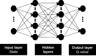
Figure 2: General neural network architecture used in the study. The neural network architecture consists of two hidden layers that take the state representation as inputs and outputs the Q-values for each available action.

3.3.4 General Training and Evaluation

To ensure an unbiased comparison with greedy optimization and DSDP, we train the RL agent using a simulated environment based on the geosteering settings mentioned in each journal. Figure 3 shows an example of the simulated environment. We train the RL agent using 51 different random seeds. We evaluate the performance of each trained agent by generating 1000 subsurface realizations from the same distributions used during training. We then compute the median of the average reward obtained by the 51 trained agents. We name this median as ”RL-Robust.” RL-Robust is calculated as follows:

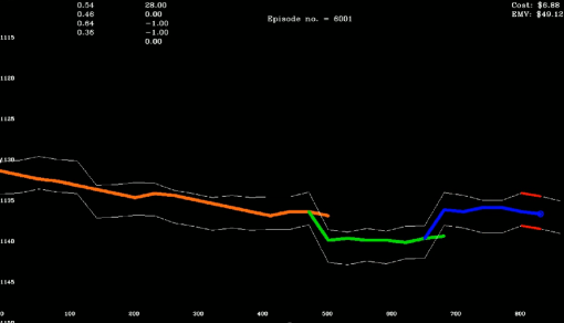
Figure 3: Illustration of the simulated environment used in the study, taken from the second example. The white lines represent the reservoir boundaries, and the colored lines represent the well trajectories. The changes in color represent sidetracks. The state representation at each step is shown on the top left-hand side, and the corresponding objective function values are displayed on the top right. The number of episodes is shown on the top middle side. The horizontal and vertical axes show the horizontal distance and the current depth in meters, respectively.

$$r_{RL}=\mathrm{Median}\left(\bar{r}_{1},\bar{r}_{2},\ldots,\bar{r}_{m}\right)$$ (7)

$$\bar{r}=\frac{\sum_{i=1}^{n}r_{i}}{n}$$ (8)

where $m$ equals to 51 and $\bar{r}$ is the average reward out of $n=1000$ subsurface realizations. In the second example, we introduce another term called the ”RL-Best,” which considers only the best average reward out of 51 trained agents. We will then compare RL results to the average reward obtained by greedy optimization and DSDP.

4 Numerical Example

In this section, we show the application of RL by studying two examples from published journals. Specifically, we analyze the studies did by Kullawan et al. in 2014 and 2018 and show how RL can optimize decision-making in complex and uncertain environments. We compare the results of RL to those obtained using greedy optimization and DSDP. By comparing these results, we can gain valuable insights into the abilities of RL to generate near-optimal decision guidance and objective results.

4.1 First Example

This subsection presents the application of RL to the geosteering environment, which is proposed by Kullawan et al. (2016a). The geosteering scenario involves drilling a horizontal well in a three-layered model with non-uniform reservoir thickness and quality. The reservoir consists of a sand layer sandwiched between shale layers and is divided into two permeability zones: a high-quality zone in the top 40 percent of the reservoir and a low-quality zone comprising the remaining 60 percent.

Given the non-uniform thickness of the reservoir, primary uncertainties in this geosteering example are the depths of the top and bottom reservoir boundaries. Signals are received from the sensor, which is located at or behind the bit, and these signals are used to determine the distance to the boundaries (at or behind the bit). These distances are then, in turn, used to update uncertainties about boundary locations ahead of the bit using a Bayesian framework. The framework assumes that the signals are accurate.

The reservoir boundaries are discretized into $N$ points. Steering decisions are made by adjusting the well inclination at every $n$ discretization point, where the change in inclination at each decision stage is restricted to no more than $5^{o}$. At each decision stage, there are 11 alternatives for inclination adjustment, ranging from $-5^{o}$ to $5^{o}$ in increments of $1^{o}$. The minimum curvature method is used to calculate the trajectory of the well at each discretization point based on the chosen inclination change.

Figure 4 shows the geosteering environment as described above. The blue line represents the well trajectory drilled in the three-layered model. The red dashed line indicates the boundary between the high-quality and low-quality reservoir zones. Decisions are made at every $n=10$ discretization point to determine the path of the well. The thickness of the reservoir varies at each discretization point, denoted by $h$. The distances from the well to the upper and lower reservoir boundaries are denoted by $DTUB$ and $DTLB$, respectively, so $h=DTUB+DTLB$. In addition, $DTHQ$ denotes the distance from the well to the high-quality zone.

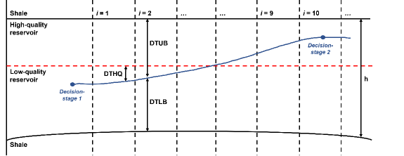
Figure 4: Illustration of the geosteering scenario, a remake based on Kullawan et al. (2016a). At every n = 10 discretization points, decisions are made to determine the well trajectory. The blue line represents the well path, while the red dashed line denotes the boundary between high and low-quality reservoir zones. The thickness of the reservoir at each discretization point is represented by $h$, while $DTUB$ and $DTLB$ denote the distances from the well to the upper and lower reservoir boundaries, respectively. Additionally, $DTHQ$ denotes the distances from the well to the high-quality zone.

The primary objective of the example is to optimize the reward function by maximizing the length of the well in the high-quality reservoir zone while at the same time avoiding reservoir exit. Two reward functions are defined for this purpose. The first reward function, $r_{1,i}$ at discretization point $i$, is:

$$r_{1,i}=14.654x_{i}^{3}-17.778x_{i}^{2}+7.2252x_{i}$$ (9)

where $x_{i}$ is the distance between the well and the nearest reservoir boundary, min($DTUB,DTLB$), normalized by the reservoir thickness $h_{i}$. The function takes its maximum value (1) when the well is placed in the middle of the reservoir ($x_{i}=0.5$). The second objective, $r_{2,i}$ at discretization point $i$, is:

$$r_{2,i}=-2\times 10^{-5}y_{i}^{2}+0.009y_{i}.$$ (10)

Here, $y_{i}$ represents the permeability of the zone, and the equation is constructed for a scenario where the maximum permeability is 200 mD, which results in a value of 1 for $y_{i}=200$.

The decision context described by Equations 9 and 10 is multi-objective with two conflicting objectives. Equation 9 indicates that placing the well in the center of the reservoir minimizes the risk of exiting the reservoir, while Equation 10 suggests that the well should be positioned in the high-quality zone to maximize its value. However, positioning the well in the high-quality zone increases the risk of drilling into the upper shale layer, which goes against the primary objective.

We thus apply a common multi-objective (Bratvold et al., 2010) decision analytic approach where the objectives are weighted. This entails computing the weighted overall reward for each of the 11 alternatives. The weighted overall reward, $r_{j}$, at decision stage $j$, is:

$$r_{j}=w_{1}\sum_{i=n*(j-1)}^{n*j-1}r_{1,i}+w_{2}\sum_{i=n*(j-1)}^{n*j-1}r_{2,i}.$$ (11)

Here, $w_{1}$ and $w_{2}$ denote the weights assigned to the two objectives, and $r_{1,i}$ and $r_{2,i}$ represent the computed reward for the $i^{th}$ discretization point for the two objectives, respectively. With $w_{1}+w_{2}=1$, the maximum value of $r_{j}$ is $n=10$.

4.1.1 RL Setting

In order to use RL method for sequential decision-making, we need to define parameters such as the action space, reward function, and state space based on the geosteering scenario. These parameters are needed for the RL agent to learn and find the optimal strategy for the scenario.

Action space. The geosteerers are engaged in decision-making to place the well optimally. They will make decisions, each with a set of alternatives, consisting of 11 discrete values ranging from -$5^{o}$ to $5^{o}$ at each decision stage. As a result, the neural network has 11 output nodes in this scenario, corresponding to the available actions that the RL agent can take.

Reward function. One of the objectives in Kullawan et al. (2016a) was to study the effect of alternative weights for each objective on the final well placement rather than the reward function. However, the RL agent is trained to maximize the reward function defined in Equation 11 for every available scenario. We compare greedy optimization and RL based on their reward function to ensure consistent training and evaluation. We use $N=100$ discretization points, and have 10 decision stages. Thus, the maximum reward for a single geosteering equals to $n*10=100$.

State space. We need to specify a state space relevant to the reward function to ensure that the RL agent has the necessary information to optimize geosteering decisions. Specifically, we provide the RL agent with $n+1$ pieces of information for reservoir thickness and the vertical distances to the reservoir boundaries and high-quality zone, with the $n$ pieces representing posterior updates ahead of the sensor location and the $+1$ piece representing the sensor reading at the current decision stage. In addition, the RL agent receives another 5 pieces of information. These include the horizontal distance from the starting point, the inclination assigned to the current discretization point, the quality of the reservoir, and the weights associated with each objective. With $n=10$ or 10 points between each decision stage, the RL agent receives 49 state information inputs, consisting of 40 posterior information pieces, 4 sensor readings, and the 5 complementary information pieces mentioned above. This configuration is referred to as ”RL-Posterior.”

In an alternative method, the Bayesian framework and posterior updates are not used. Instead, the RL agent receives sensor readings from $n$ discretization points behind the sensor location, while other complementary information is identical in both methods. This method can help us show the capacity of RL (DQN) to optimize the problem by implicitly predicting the boundaries ahead of the sensor location without the need for potentially costly Bayesian computations. This configuration is referred to as ”RL-Sensor.”

The state representation of both RL agents is summarized in Table 2. The first two rows correspond to the $n+1$ information described earlier. However, the important distinction lies in the subscript notation of the information. For the RL-Posterior method, the information range from the sensor location $i$ to $n$ discretization points ahead, while for the RL-Sensor method, the information starts from $n$ discretization points behind the sensor location $i$. The remaining information, including $Inc_{i}$ representing the inclination at the current point, $i$ denoting the current discretization point (or equivalently, the horizontal distance from the starting point), $y$ representing the reservoir quality, and $w_{1}$ and $w_{2}$ denoting the weights of each objective, remain consistent across both agents.

Table 2: Comparison of the state representations of the two RL methods

Model	State Representation
RL-Posterior	{$DTUB_{i}$,…, $DTUB_{i+n}$, $DTLB_{i}$,…, $DTLB_{i+n}$, $DTHQ_{i}$,…, $DTHQ_{i+n}$, $h_{i}$,…, $h_{i+n}$, $Inc_{i}$, $i$, $y$, $w_{1}$, $w_{2}$}
RL-Sensor	{$DTUB_{i-n}$,…, $DTUB_{i}$, $DTLB_{i-n}$,…, $DTLB_{i}$, $DTHQ_{i-n}$,…, $DTHQ_{i}$, $h_{i-n}$,…, $h_{i}$, $Inc_{i}$, $i$, $y$, $w_{1}$, $w_{2}$}

4.1.2 Training Results

Following Kullawan et al. (2016a), we split the example into two scenarios based on the reservoir quality disparity between the two zones. We train the RL agent to optimize both scenarios simultaneously to avoid the need to train the RL agent multiple times. It could also show the generalizability of the resulting decision-making policy.

Figure 5 visually shows the outcomes of training a single seed of the two RL methods: the RL-Posterior and RL-Sensor, in the first example. The red lines represent the RL-Posterior method, while the blue lines represent the RL-Sensor method. The figure presents the evolution of the percentage of each individual objective, specifically the reservoir contact and the high-quality zone percentages, alongside the rewards obtained during the geosteering operation. The figure is constructed by taking the average of the numbers (percentages and rewards) obtained during the last 100 training episodes. This approach provides a smoothed representation of the performance of an RL decision-making agent and helps mitigate the effects of short-term fluctuations.

Both RL agents gradually improve their decision-making policies throughout the training, as seen by the overall increase in all objectives and rewards. The reservoir contact objective, which initially stands at less than 40 percent during the early stage of training, improves significantly for both agents, reaching approximately 90 percent by the end of the training. Additionally, both agents increase the high-quality zone percentage from 20 percent to approximately 60 percent after the training sequence.

Regarding the rewards, it is important to address the presence of large negative values observed at the beginning of the training. These values are caused by the reward function associated with the first objective. The reward function assigns a large negative number when the well trajectory is significantly distant from the target zone, resulting in the noticeable negative values shown in the figure. However, as the RL agent learns from experience, the rewards gradually increase and remain above zero when the training sequence ends.

While the difference between the two agents may appear negligible at first glance, closer examination reveals a slight advantage for the RL-Sensor method regarding the high-quality zone objective. It is important to note that the figure shown is based on a single training seed, and a more comprehensive comparison will be done in the subsequent section. In that section, the performance of all training seeds will be averaged, providing a more robust comparison of the relative performance between the RL agents.

Another important aspect is the computational cost of training a single seed. The RL-Posterior method requires approximately 2500 seconds to complete the training sequence, whereas the RL-Sensor method completes the training in a significantly shorter time, around 500 seconds. This substantial difference in training duration is caused by the utilization of the Bayesian framework in the RL-Posterior method, which introduces additional computational costs. On the other hand, the RL-Sensor method, which does not rely on the Bayesian framework, offers a more computationally efficient alternative.

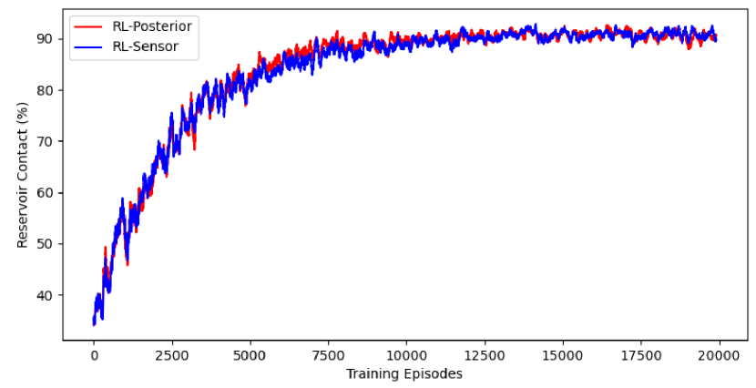
(a) Reservoir Contact

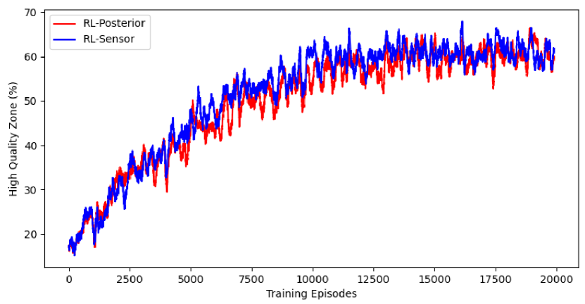
(b) High Quality Zone

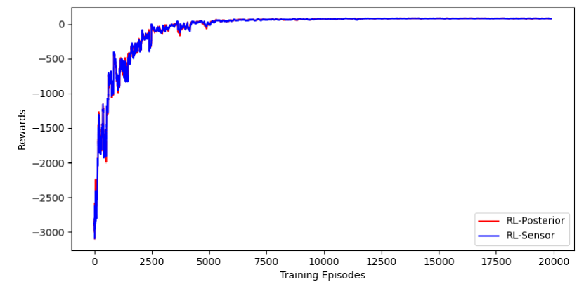
(c) Rewards

Figure 5: Evolution of individual objectives (reservoir contact and high-quality zone percentages) and the overall rewards of two RL agents during training. The red lines represent the RL-Posterior method, while the blue lines represent the RL-Sensor method. The figure reflects the average from the last 100 training episodes.

4.1.3 Evaluation Results

We generate 1000 different reservoir realizations for evaluation purposes, ensuring that the results represent various scenarios described below. This subsection presents the results of the first study, while the subsequent subsection will focus on discussing those results in more detail.

Scenario 1. The permeability of the high-quality zone is 200 mD, whereas the permeability of the low-quality zone is 100 mD. There is a distinction in quality, although it is not substantial. Consequently, the first objective is assigned a greater weight, with $w_{1}=0.67$ and $w_{2}=0.33$.

Table 3: Scenario 1 - Average results for greedy optimization and Median results for both RL-agents

Methods	Rewards	Reservoir contact (%)	High quality (%)
Greedy	71.44	87.90	43.00
RL-Posterior*	85.25	92.86	44.06
RL-Sensor*	85.79	92.86	46.77

• *RL-Robust

Table 3 presents the results of greedy optimization and two RL methods, RL-Posterior and RL-Sensor. The median reward of the RL-Posterior method is 85.25 out of 100, representing a significant improvement of 19.34 percent over the greedy optimization. Meanwhile, the RL-Sensor method achieves a slightly higher median reward of 85.79. Furthermore, both RL agents yield better well placement by achieving higher figures on both objectives.

Scenario 2. The permeability of the high-quality zone is 200 mD, while the permeability of the low-quality zone is 20 mD. Given the more substantial difference in quality compared to scenario 1, it is important to position the well in the top portion of the reservoir. Therefore, the weight for the second objective is greater than in the first objective, with $w_{1}=0.41$ and $w_{2}=0.59$.

Table 4: Scenario 2 - Average results for greedy optimization and Median results for both RL-agents

Methods	Rewards	Reservoir contact (%)	High quality (%)
Greedy	55.57	82.50	53.20
RL-Posterior*	73.76	89.85	65.62
RL-Sensor*	74.21	88.65	70.22

• *RL-Robust

Table 4 presents the average results of greedy optimization and median results of both RL configurations in scenario 2. Similar to scenario 1, the RL-Posterior and RL-Sensor methods outperform greedy optimization in all three metrics, with higher rewards, reservoir contact percentage, and high-quality percentage.

The primary objective in this scenario is to position the well inside the high-quality zone. As a result, the well is placed closer to the upper reservoir borders, which increases the probability of exiting the reservoir, leading to a relatively low reward from the first reward function. Furthermore, the low-quality zone in scenario 2 has a lower permeability value than in scenario 1, reducing the overall reward of scenario 2. Nevertheless, the table illustrates that RL has higher value in scenario 2 than in scenario 1, with a 32.74 percent increase for the RL-Posterior method and a 33.55 percent increase for the RL-Sensor method.

4.1.4 Discussion

The RL methods used in this study yield significantly better results than greedy optimization. The superior performance of the RL methods is attributed to their ability to learn from experience and explore different strategies to maximize the reward. By contrast, greedy optimization only considers the immediate reward and does not consider future decisions and future learning.

The results also show that the RL-Sensor method consistently outperforms the RL-Posterior method in terms of median reward across all scenarios. Although the difference in performance is insignificant, it is consistent, and the RL-Sensor method achieves the results without requiring posterior updates, suggesting that it can implicitly anticipate reservoir boundaries using the sensor readings behind the sensor location. One plausible explanation for the observed difference is that the posterior updates derived from the Bayesian framework might contain inaccuracies and errors. Although the implicit predictions from RL can also suffer from similar issues, the superior performance of the RL-Sensor method implies that the implicit predictions provide more accurate approximations compared to the posterior updates.

Moreover, eliminating the Bayesian framework in the RL-Sensor method reduces the training time for a single seed from 2500 to 500 seconds while still achieving superior results. With a computational cost that is 5 times cheaper, the RL-Sensor method remains the superior method even when its results are slightly worse than those of the RL-Posterior method. Therefore, we exclusively use the RL-Sensor method for the second example described in the following subsection.

4.2 Second Example

In this section, we show the application of the RL-Sensor method to an example previously shown by Kullawan et al. (2018). Their study used greedy optimization and DSDP to optimize a geosteering scenario in thin and faulted reservoirs. The geosteering context for this example is similar to the first example, where a horizontal well is drilled in a three-layered reservoir model consisting of a sand reservoir sandwiched between shale layers.

The example considers a constant reservoir thickness and uniform quality, reducing uncertainties in this case to the depths of the upper reservoir boundary and the location and displacement of faults. The prior knowledge of the depth of boundaries is combined with fault information, such as the number of faults, expected fault displacement, and possible fault location. As in the first example, Kullawan et al. (2018) uses a Bayesian framework to update the combined prior information based on real-time sensor data. Additionally, the study assumes that the real-time information is accurate.

We use the same prior geomodel and fault uncertainty parameters as Kullawan et al. (2018), shown in Figure 6. The reservoir boundaries are discretized into 30 points ($N=30$) spaced 30 meters apart, with solid black lines indicating the expected upper and lower boundaries of the reservoir. Green dashed lines represent potential fault displacements, with uncertainty modeled using a normal distribution. Red dashed lines indicate possible fault locations, with uncertainty modeled using discrete uniform distributions. For instance, the first fault has an estimated displacement of 3 meters, with a standard deviation of 1 meter, and may be located 120 meters, 150 meters, or 180 meters from the first discretization point.

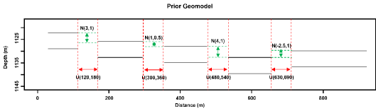
Figure 6: Illustration of prior geomodel and fault uncertainties remade based on Kullawan et al. (2018). The expected upper and lower boundaries are shown as solid black lines. Uncertainty in potential fault displacements is represented by green dashed lines, modeled using a normal distribution. Uncertainty in possible fault locations is represented by red dashed lines, modeled using discrete uniform distributions.

In this geosteering setting, there are 29 decision stages, and steering decisions are made at every discretization point ($n=1$) by directly modifying the well depth without using the minimum curvature method. At each decision stage $j$, 5 options are available for altering the well depth, ranging from $-0.5$-m TVD to $0.5$-m TVD with a $0.25$-m TVD increase. Additionally, sidetracking can be done if the well exits the reservoir after deciding to modify or maintain the well depth. We refer to it as the default setup, where a steering decision is followed by a sidetrack decision. Sidetracking can ensure that the well is drilled towards the center of the boundary. However, it incurs additional costs. In other words, sidetracking represents a trade-off between future gain and present increased expense.

Figure 7 illustrates how each alternative changes the well depth at each decision node. In this example, the blue line represents the well trajectory, which has exited the reservoir boundaries, represented by the black lines. When making a steering decision, the decision maker can adjust the well depth using any of the 5 alternatives represented by the blue arrows. On the other hand, if the decision maker chooses to execute a sidetrack, the well is taken back to the previous decision stage and drilled directly to the middle of the reservoir boundaries for the next decision stage, as shown by the red line and arrows. The blue dashed line in the figure indicates that the previous well trajectory is discarded as if it had never been drilled.

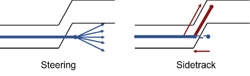
Figure 7: Illustration of alternatives from the second example. The blue line represents the well trajectory, while the black lines represent the reservoir boundaries. The decision maker can make a steering decision using the 5 alternatives represented by the blue arrows. If the sidetrack is chosen, the well is taken back to the previous decision stage and drilled directly to the middle of the reservoir boundaries for the next decision stage, as shown by the red line and arrows.

In this example, we aim to optimize the reward of a geosteering project by maximizing reservoir contact and minimizing operating costs. To this end, the setting uses a reward function $r_{j}$ that combines the values $v_{j}$ and operating costs $c_{j}$ at each decision stage $j$. Specifically, $r_{j}$ is defined as:

$$r_{j}=v_{j}-c_{j}.$$ (12)

Here, $v_{j}$ represents the value given the location of the well, which is equal to the production value $v_{prod}$ if the well is located within the reservoir and 0 otherwise. The operating cost $c_{j}$ is the sum of the drilling cost $c_{d}$, and the sidetrack cost $c_{ST}$ if sidetracking is done. We use values of $v_{prod}$ ranging from 0.5 to 4.0, with $c_{d}$ and $c_{ST}$ held constant at 0.0625 and 2.567, respectively. Consequently, for 29 decision stages, the maximum value of a geosteering project is $29\cdot v_{prod}$, and the minimum operating cost is $29\cdot c_{d}=1.81$.

4.2.1 RL Setting

As in the first example, we need to specify the following three parameters from the geosteering scenario to use RL for sequential decision-making:

Action space. In the default setup, there are two decision nodes in one decision stage: the first for modifying the drill bit depth and the second for performing a sidetrack. However, this configuration can lead to sub-optimal results for specific scenarios when we use RL. For example, when the value $v_{prod}$ is less than the sidetrack cost $c_{ST}$, an RL decision-making agent using two decision nodes may follow a greedy decision-making policy and decline to do a sidetrack. Conversely, when $v_{prod}$ exceeds $c_{ST}$, the agent will always choose to sidetrack, irrespective of the actual value of the well. Thus, using two decision nodes could limit the ability of the RL agent to make optimal decisions regarding sidetracking.

To address this issue, we adapt the action space to include a single decision node with 6 alternatives, 5 of which correspond to adjustments in the drill bit depth, while the sixth alternative is for performing a sidetrack. As a result, the neural network for the second scenario contains 6 output nodes.

However, this modification introduces another issue where the sidetrack alternative is consistently available, whereas in the default setup, the sidetrack option is restricted when the drill bit is already within the reservoir. To address this issue, we temporarily force the RL agent to disregard the sidetrack alternative when it is unnecessary. On the other hand, if the drill bit exits the reservoir, every alternative is available for the RL agent. Hence, it can either execute a sidetrack or continue making steering decisions for the subsequent decision stages. This approach enables the agent to make appropriate decisions based on the current location of the drill bit. As a result, we can evaluate the ability of the RL agent to handle both steering and sidetrack decisions effectively.

Reward function. The reward function used in the RL configuration remains unchanged and is the same as the default setting, as shown in Equation 12. Thus, the RL agent receives a reward $r_{j}$ after each decision stage. Moreover, we did not alter the evaluation method since the default setting already used a consistent approach that compared the performance of different methods based on their total reward function, which is defined as the sum of rewards over all decision stages, i.e., $\sum r_{j}$.

State space. As the second example assumes a constant reservoir thickness and homogeneous reservoir quality, the RL-Sensor method requires less information about the reservoir than in the first. We provide an RL decision-making agent $n+1$ information on vertical distances between the well trajectory and reservoir boundaries. Additionally, with the inclusion of faults and sidetracks in the geosteering setting, we also inform the agent about the possible zone and the expected displacement of the subsequent fault.

Furthermore, it is important for the agent to know whether the well trajectory is inside or outside the reservoir. We also inform the agent about its horizontal distance from the initial point and the value of the current geosteering project. Consequently, the RL-Sensor method gathers 9 pieces of information at each decision stage, which serve as inputs for the neural network.

4.2.2 Training Results

Figure 8 illustrates the training outcomes of the RL-Sensor method in the second example. The training for a single seed requires approximately 20 minutes. Similar to the first example, the figure presents the evolution of individual objectives, specifically the reservoir contact and the operating cost, alongside the overall rewards obtained during the geosteering operation. The figure is also constructed by taking the average obtained during the last 100 training steps. Moreover, the training also considers the number of scenarios the example has. The scenario in this example depends on the production value $v_{prod}$ that ranges from 0.5 to 4.

The figure illustrates the evolution of the RL-sensor method decision-making policy. Over time, the RL-Sensor method improves the reservoir contact from an initial percentage of 65 to approximately 90 percent. Simultaneously, it reduces the operating cost from a starting cost of 8 to around 3, which correlates with decreased sidetrack operations. In other words, the RL-Sensor method gradually learns to make a better steering decision, reducing the need for frequent sidetrack operations.

The evolution of the average rewards shows a higher fluctuation level than in the previous example. This increased variability is primarily attributed to the influence of the production value, $v_{prod}$, which is determined by the random sampling procedures used during the training sequence. For instance, when $v_{prod}$ is set to 0.5, the maximum reward attainable by a decision-making agent in a single training episode is $29\times 0.5-1.81=12.69$. Conversely, when $v_{prod}$ equals 4, the maximum achievable reward becomes $29\times 4-1.81=114.19$, approximately 10 times larger than the other scenario.

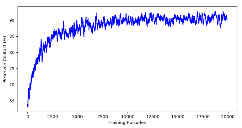
(a) Reservoir Contact

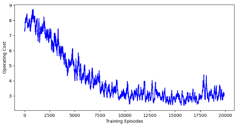
(b) Operating Cost

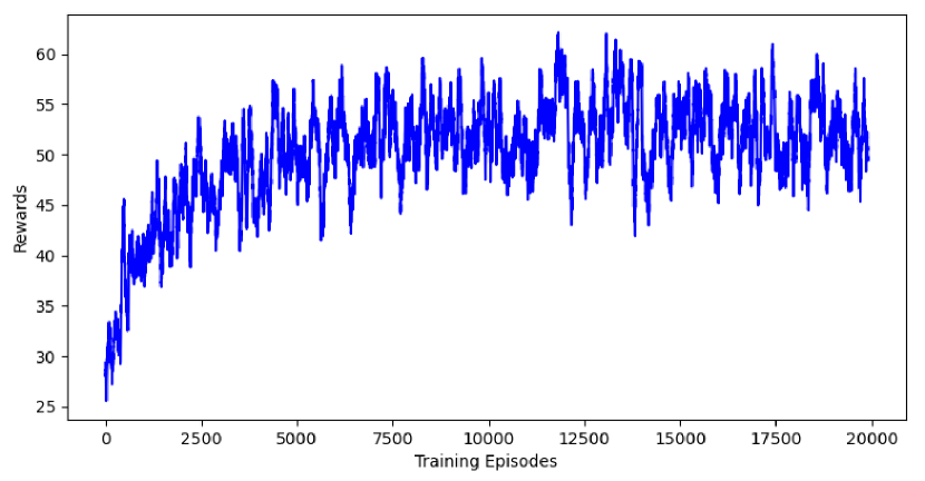
(c) Rewards

Figure 8: Evolution of individual objectives (reservoir contact and operating costs) and the overall rewards of the RL-Sensor method during training. The figure reflects the average from the last 100 training episodes

4.2.3 Evaluation Results

We run 1000 simulations of the geomodel shown in Figure 6 to evaluate the performance of different methods by studying the impact of varying $v_{prod}$ values on the rewards, reservoir contact, and operating cost. This subsection presents the results, while the subsequent subsection will provide a discussion and analysis of the results.

Scenario 1. $v_{prod}=0.5$, resulting in a very expensive sidetrack cost and making sidetrack decisions less favorable than steering decisions ($v_{prod}<<<c_{ST}$). Table 5 shows the rewards, reservoir contact, and operating cost of all three methods for scenario 1.

Table 5: Scenario 1 - Results for Greedy Optimization, DSDP, RL-Sensor Robust, and RL-Sensor Best

Methods	Rewards	Reservoir contact (%)	Operating Cost
Greedy	8.33	69.94	1.81
DSDP	11.40	92.47	2.01
RL-Sensor	11.50	91.80	1.81
RL-Sensor Best	11.72	93.37	1.82

At $v_{prod}=0.5$, greedy optimization never chooses to do a sidetrack, as suggested by its minimum operating cost of 1.81. It achieves the lowest average reservoir contact of 69.94 percent and, unsurprisingly, the lowest average reward among the other methods, at 8.33. On the other hand, the DSDP achieves a significantly higher reservoir contact of 92.47 percent compared to greedy optimization.

The RL-Sensor method achieves a high reservoir contact of 91.80 percent while maintaining a minimal cost of operation. In this scenario, the RL-Sensor decision-making policy is similar to greedy optimization in that it does not do sidetrack operations and relies only on steering decisions. Despite not performing any sidetracks, the results show that the RL-Sensor method, with a median reward of 11.50, slightly outperforms the DSDP. We also include RL-Sensor Best, and it further outperforms the DSDP with a reservoir contact percentage of 93.37 and a median reward of 11.72.

Scenario 2. $v_{prod}=2$, which is still slightly lower than the sidetrack cost ($v_{prod}<c_{ST}$). Table 6 shows the rewards, reservoir contact, and operating cost of all three methods for scenario 2.

Table 6: Scenario 2 - Results for Greedy Optimization, DSDP, RL-Sensor Robust, and RL-Sensor Best

Methods	Rewards	Reservoir contact (%)	Operating Cost
Greedy	38.76	69.96	1.81
DSDP	51.93	95.02	3.18
RL-Sensor	52.31	96.54	3.68
RL-Sensor Best	52.90	96.17	2.87

The decision-making policy of greedy optimization remains the same at $v_{prod}$ = 2 as the production value is still below the sidetrack cost. As a result, greedy optimization still achieves the minimum operating cost with no improvement in reservoir contact. Similar to the first scenario, its average reward is the lowest among all methods at 38.76. On the other hand, the DSDP performs more sidetrack operations than in the previous scenario, resulting in a higher cost. However, this method achieves an average reward of 51.93, considerably better than greedy optimization.

Like the DSDP, the RL-Sensor method incurs a higher operating cost than in scenario 1 due to performing more sidetrack operations. Specifically, the decision-making policy of the RL-Sensor method leads to an operating cost of 3.68 while achieving a high reservoir contact of 96.54 percent. These results show the ability of the RL-Sensor method to strike a balance between maximizing reservoir contact and minimizing operating cost, even when the production value is still below the sidetrack cost. Compared to the DSDP, the RL-Sensor method yields a slightly higher median reward of 52.31. The RL-Sensor Best outperforms all other methods, achieving the highest average reward of 52.90 with a reservoir contact of 96.17 percent and an operating cost of 2.87.

Scenario 3. $v_{prod}=4$, resulting in a very cheap sidetrack cost and making it, when available, more favorable than steering decisions ($v_{prod}>>>c_{ST}$). Table 7 shows the rewards, reservoir contact, and operating cost of all three methods for scenario 3.

Table 7: Scenario 3 - Results for Greedy Optimization, DSDP, RL-Sensor Robust, and RL-Sensor Best

Methods	Rewards	Reservoir contact (%)	Operating Cost
Greedy	104.44	98.26	9.54
DSDP	107.73	98.26	6.25
RL-Sensor	107.46	97.64	5.80
RL-Sensor Best	109.10	96.83	3.23

At $v_{prod}=4$, greedy optimization maximizes immediate reward by performing a sidetrack whenever the well exits the reservoir, resulting in 98.26 percent reservoir contact. However, this strategy comes at a significant increase in operating costs. On the other hand, the DSDP reaches the same reservoir contact with fewer sidetracks, resulting in a higher average reward of 107.73 compared to 104.4 for greedy optimization.

The RL-Sensor method achieves a reservoir contact of 97.64 percent but at a lower operating cost than the other methods. Its average reward of 107.46 is only 0.25 lower than the DSDP. However, this is the only scenario where the RL-Sensor method cannot outperform the DSDP, which occurs when the DSDP provides the least additional value over greedy optimization. Nonetheless, the RL-Sensor Best achieves the highest reward among all methods, with a reservoir contact of 96.83 percent and an operating cost of 3.23.

4.2.4 Discussion

The results from the second example provide additional evidence supporting our results that the RL-Sensor method outperforms greedy optimization. This example effectively demonstrates the divergence in decision-making between the two methods. The greedy optimization makes sidetrack decisions based solely on the value of $v_{prod}$, whereby if it is lower than $v_{ST}$, greedy optimization always chooses to forego the sidetrack. On the other hand, greedy optimization always chooses to sidetrack if $v_{prod}$ is higher than $v_{ST}$. On the other hand, the sidetrack and overall decision-making policy of the RL-Sensor method consider future values, leading to substantially higher rewards.

The results from all studied scenarios also indicate that the performance of the RL-Sensor method is comparable to that of the DSDP, which is considered the quasi-optimal solution to the dynamic programming. In several cases, the RL agent even outperforms the DSDP. One possible explanation is that RL does not require discretization, unlike the DSDP, which may lead to better performance. The absence of discretization in RL may enable it to achieve more accurate results by avoiding information loss during the discretization process.

It is worth noting that there is one scenario where the RL-Sensor method does not outperform the DSDP, although the difference is not statistically significant. This scenario is where $v_{prod}$ is higher than $v_{ST}$, leading to a preference for sidetracking over steering if the well exits the reservoir. One plausible explanation is that sidetracking allows to adjust the well trajectory by returning it to the center of the boundaries, thus mitigating the effects of information loss caused by discretization.

In addition to comparable performance, the RL agent substantially reduces long-term computational costs compared to the DSDP. Specifically, after training for approximately 20 minutes, the RL agent can evaluate 1000 reservoir realizations in less than 10 seconds. On the other hand, the current discretization setup requires the DSDP to evaluate one realization in 15-20 seconds. The DSDP would take 4-5 hours to evaluate the same number of reservoir realizations. These results suggest that RL may produce a more computationally cost-efficient solution to the geosteering scenario than the DSDP.

5 Conclusions

This study introduces and illustrates the application of reinforcement learning (RL) as a flexible, robust, and computationally efficient sequential decision-making tool in two distinct geosteering environments.

The results from the first example indicate that RL-Posterior method suggests decisions that lead to significantly improved value function results compared with greedy optimization, with a 19 to 33 percent increase depending on the scenario. In addition to the RL-Posterior method, we introduce an alternative method called the RL-Sensor method. The RL-Sensor method ignores the posterior updates and relies on the inputs to the Bayesian framework. The RL-Sensor method offers slightly better rewards than the RL-Posterior method while significantly reducing the computational cost. Specifically, the computation time is reduced from 2500 seconds to 500 seconds.

Our results from the second example show that RL provides comparable rewards to the DSDP, which we define as the quasi-optimal solution to dynamic programming. Notably, RL achieves these results with significantly less computational cost. Specifically, the computation time for training an RL decision-making agent and evaluating 1000 geomodel realizations is approximately 20 minutes (training) + 10 seconds (evaluating). On the other hand, the DSDP requires 15 to 20 seconds for each realization, resulting in approximately 4-5 hours to evaluate 1000 realizations. These results suggest that RL is a promising alternative to the DSDP for optimizing geosteering decision-making problems where computational efficiency is important.

We also highlight the ease of implementing RL method, which is independent of the environment. The challenge lies in defining the appropriate state representation to optimize the reward function for each environment. As shown in our study, certain information may be relevant in one setting but not another. For instance, inclination is included as one of the states in the first environment but not in the second. Overall, the results show the flexibility and potential of RL-based methods in optimizing complex geosteering decision-making problems in various environments.

Our study assumes that the primary source of uncertainty in both environments is the reservoir boundaries and that there are no errors in the sensor readings. In reality, geosteering decisions are made in the face of multiple uncertainties, and sensor readings have different levels of precision. To address this limitation, future studies could explore the ability of RL in providing an efficient and robust geosteering decision-making strategy under any number of uncertainties and can also deal with sensor reading errors. This would provide a more realistic evaluation of the performance of RL method and its potential for decision optimization in practical applications.

Declaration of generative AI and AI-assisted technologies in the writing process

During the preparation of this work, the author(s) used ChatGPT in order to improve the readability. After using this tool/service, the author(s) reviewed and edited the content as needed and take(s) full responsibility for the content of the publication.

References

- Alyaev et al. (2021) Alyaev, S., Ivanova, S., Holsaeter, A., Bratvold, R.B., Bendiksen, M., 2021. An interactive sequential-decision benchmark from geosteering. Applied Computing and Geosciences 12, 100072. doi:https://doi.org/10.1016/j.acags.2021.100072.
- Alyaev et al. (2019) Alyaev, S., Suter, E., Bratvold, R.B., Hong, A., Luo, X., Fossum, K., 2019. A decision support system for multi-target geosteering. Journal of Petroleum Science and Engineering 183, 106381. doi:https://doi.org/10.1016/j.petrol.2019.106381.
- Bahlawan et al. (2019) Bahlawan, H., Morini, M., Pinelli, M., Spina, P.R., 2019. Dynamic programming based methodology for the optimization of the sizing and operation of hybrid energy plants. Applied Thermal Engineering 160, 113967. doi:https://doi.org/10.1016/j.applthermaleng.2019.113967.
- Bellman (1966) Bellman, R., 1966. Dynamic programming. Science 153, 34–37. doi:10.1126/science.153.3731.34.
- Bratvold et al. (2010) Bratvold, R., Begg, S., of Petroleum Engineers (U.S.), S., 2010. Making Good Decisions. Society of Petroleum Engineers. URL: https://books.google.co.id/books?id=d1kbkgAACAAJ.
- Chen et al. (2014) Chen, Y., Lorentzen, R.J., Vefring, E.H., 2014. Optimization of Well Trajectory Under Uncertainty for Proactive Geosteering. SPE Journal 20, 368–383. doi:10.2118/172497-PA.
- Dixit and ElSheikh (2022) Dixit, A., ElSheikh, A.H., 2022. Stochastic optimal well control in subsurface reservoirs using reinforcement learning. Engineering Applications of Artificial Intelligence 114, 105106. doi:10.1016/j.engappai.2022.105106.
- He et al. (2022) He, J., Tang, M., Hu, C., Tanaka, S., Wang, K., Wen, X.H., Nasir, Y., 2022. Deep Reinforcement Learning for Generalizable Field Development Optimization. SPE Journal 27, 226–245. doi:10.2118/203951-PA.
- Kristoffersen et al. (2021) Kristoffersen, B.S., Silva, T.L., Bellout, M.C., Berg, C.F., 2021. Efficient well placement optimization under uncertainty using a virtual drilling procedure. Computational Geosciences 26, 739–756. doi:10.1007/s10596-021-10097-4.
- Kullawan et al. (2016a) Kullawan, K., Bratvold, R., Bickel, J., 2016a. Value creation with multi-criteria decision making in geosteering operations. SPE Hydrocarbon Economics and Evaluation Symposium doi:10.2118/169849-MS.
- Kullawan et al. (2018) Kullawan, K., Bratvold, R., Bickel, J., 2018. Sequential geosteering decisions for optimization of real-time well placement. Journal of Petroleum Science and Engineering 165, 90–104. doi:https://doi.org/10.1016/j.petrol.2018.01.068.
- Kullawan et al. (2016b) Kullawan, K., Bratvold, R.B., Nieto, C.M., 2016b. Decision-Oriented Geosteering and the Value of Look-Ahead Information: A Case-Based Study. SPE Journal 22, 767–782. doi:10.2118/184392-PA.
- Liu et al. (2018) Liu, H., Zhu, D., Liu, Y., Du, A., Chen, D., Ye, Z., 2018. A reinforcement learning based 3d guided drilling method: Beyond ground control, in: Proceedings of the 2018 VII International Conference on Network, Communication and Computing, Association for Computing Machinery, New York, NY, USA. p. 44–48. doi:10.1145/3301326.3301374.
- Mnih et al. (2015) Mnih, V., Kavukcuoglu, K., Silver, D., Rusu, A.A., Veness, J., Bellemare, M.G., Graves, A., Riedmiller, M., Fidjeland, A.K., Ostrovski, G., Petersen, S., Beattie, C., Sadik, A., Antonoglou, I., King, H., Kumaran, D., Wierstra, D., Legg, S., Hassabis, D., 2015. Human-level control through deep reinforcement learning. Nature 518, 529–533. doi:https://doi.org/10.1038/nature14236.
- Nasir and Durlofsky (2022) Nasir, Y., Durlofsky, L.J., 2022. Deep reinforcement learning for optimal well control in subsurface systems with uncertain geology. arXiv preprint doi:10.48550/ARXIV.2203.13375.
- Paszke et al. (2019) Paszke, A., Gross, S., Massa, F., Lerer, A., Bradbury, J., Chanan, G., Killeen, T., Lin, Z., Gimelshein, N., Antiga, L., Desmaison, A., Kopf, A., Yang, E., DeVito, Z., Raison, M., Tejani, A., Chilamkurthy, S., Steiner, B., Fang, L., Bai, J., Chintala, S., 2019. Pytorch: An imperative style, high-performance deep learning library, in: Advances in Neural Information Processing Systems 32. Curran Associates, Inc., pp. 8024–8035.
- Powell (2009) Powell, W.B., 2009. What you should know about approximate dynamic programming. Nav. Res. Logist. 56, 239–249. doi:https://doi.org/10.1002/nav.20347.
- Puterman (1990) Puterman, M.L., 1990. Chapter 8 markov decision processes, in: Stochastic Models. Elsevier. volume 2 of Handbooks in Operations Research and Management Science, pp. 331–434. doi:https://doi.org/10.1016/S0927-0507(05)80172-0.
- Sutton and Barto (2018) Sutton, R.S., Barto, A.G., 2018. Reinforcement Learning: An Introduction. A Bradford Book, Cambridge, MA, USA.
- Tsitsiklis and Van Roy (1997) Tsitsiklis, J., Van Roy, B., 1997. An analysis of temporal-difference learning with function approximation. IEEE Transactions on Automatic Control 42, 674–690. doi:10.1109/9.580874.
- Wang et al. (2015) Wang, X., He, H., Sun, F., Zhang, J., 2015. Application study on the dynamic programming algorithm for energy management of plug-in hybrid electric vehicles. Energies 8, 3225–3244. doi:10.3390/en8043225.
- Zaccone et al. (2018) Zaccone, R., Ottaviani, E., Figari, M., Altosole, M., 2018. Ship voyage optimization for safe and energy-efficient navigation: A dynamic programming approach. Ocean Engineering 153, 215–224. doi:https://doi.org/10.1016/j.oceaneng.2018.01.100.