Binary Quantification and Dataset Shift:
An Experimental Investigation

Abstract

Quantification is the supervised learning task that consists of training predictors of the class prevalence values of sets of unlabelled data, and is of special interest when the labelled data on which the predictor has been trained and the unlabelled data are not IID, i.e., suffer from dataset shift. To date, quantification methods have mostly been tested only on a special case of dataset shift, i.e., prior probability shift; the relationship between quantification and other types of dataset shift remains, by and large, unexplored. In this work we carry out an experimental analysis of how current quantification algorithms behave under different types of dataset shift, in order to identify limitations of current approaches and hopefully pave the way for the development of more broadly applicable methods. We do this by proposing a fine-grained taxonomy of types of dataset shift, by establishing protocols for the generation of datasets affected by these types of shift, and by testing existing quantification methods on the datasets thus generated. One finding that results from this investigation is that many existing quantification methods that had been found robust to prior probability shift are not necessarily robust to other types of dataset shift. A second finding is that no existing quantification method seems to be robust enough to dealing with all the types of dataset shift we simulate in our experiments. The code needed to reproduce all our experiments is publicly available at https://github.com/pglez82/quant_datasetshift.

1 Introduction

Quantification (variously called learning to quantify, or class prior estimation, or class distribution estimation – see (Esuli et al., 2023; González et al., 2017) for overviews) is a supervised learning task concerned with estimating the prevalence values (or relative frequencies, or prior probabilities) of the classes in a sample of unlabelled datapoints, using a predictive model (the quantifier) trained on labelled datapoints.

A straightforward solution to the quantification problem can be obtained by (i) using a classifier to issue label predictions for the unlabelled datapoints in the sample, (ii) counting how many datapoints have been attributed to each class, and (iii) reporting the relative frequencies. This method is typically known as Classify and Count (CC). However, unless the classifier is a perfect one, CC is known to deliver suboptimal solutions (Forman, 2005). One reason (but not the only one) is that CC tends to inherit the bias of the classifier; for example, in binary quantification problems (i.e., when there are only two mutually exclusive classes), if the classifier has a tendency to produce more (resp., fewer) false positives than false negatives, CC tends to overestimate (resp., underestimate) the prevalence of the positive class.

Since the term “quantification” was coined by Forman (2005), quantification has come to be recognised as a task in its own right and is, by now, no longer considered as a mere by-product of classification. Quantification finds applications in many areas whose primary focus is the analysis of data at the aggregate level (rather at the level of the individual datapoint), such as market research (Esuli and Sebastiani, 2010), the social sciences (Hopkins and King, 2010), ecological modelling (Beijbom et al., 2015), and epidemiology (King and Lu, 2008), among many others.

A common trait of all these applications is that all of them emerge from the need to monitor evolving class distributions, i.e., situations in which the class distribution of the unlabelled data may differ from the one of the training data. In other words, these situations are characterised by a type of dataset shift (Moreno-Torres et al., 2012; Quiñonero-Candela et al., 2009), i.e., the phenomenon according to which, in a supervised learning context, the training data and the unlabelled data are not IID. Dataset shift comes in different flavours; the ones that have mostly been discussed in the literature are (i) prior probability shift, which has to do with changes in the class prevalence values; (ii) covariate shift, which concerns changes in the distribution of the covariates (i.e., features); and (iii) concept shift, which has to do with changes in the functional relationship between covariates and classes. We provide more formal definitions of dataset shift and its subtypes in the sections to come.

Since quantification aims at estimating class prevalence, most experimental evaluations of quantification systems (see, e.g., (Barranquero et al., 2015; Bella et al., 2010; Esuli et al., 2018; Forman, 2008; Hassan et al., 2020; Milli et al., 2013; Moreo and Sebastiani, 2022; Pérez-Gállego et al., 2019; Schumacher et al., 2021)) have focused on situations characterised by prior probability shift, while the other two types of shift mentioned above have not received comparable attention. A question then naturally arises: How do existing quantification methods fare when confronted with types of dataset shift other than prior probability shift?

This paper offers a systematic exploration of the performance of existing quantification methods under different types of dataset shift. To this aim we first propose a fine-grained taxonomy of dataset shift types; in particular, we pay special attention to the case of covariate shift, and identify variants of it (mostly having to do with additional changes in the priors) that we contend to be of special relevance in quantification endeavours, and that are understudied. We then follow an empirical approach, devising specific experimental protocols for simulating all the types of dataset shift that we have identified, at various degrees of intensity and in a tightly controlled manner. Using the experimental setups generated by means of these protocols, we then test a number of existing quantification methods; here, the ultimate goal we pursue is to better understand the relative merits and limitations of existing quantification algorithms, to understand the conditions under which they tend to perform well, and to identify the situations in which they instead tend to generate unreliable predictions.

The rest of this paper is organised as follows. In Section 2, we discuss previous work on establishing protocols to recreate different types of dataset shift, with special attention to work done in the quantification arena, and the (still scarce) work aimed at drawing connections between quantification and different types of dataset shift. In Section 3, we illustrate our notation and provide definitions of relevant concepts and of the quantification methods we use in this study. Section 4 goes on by introducing formal definitions of the types of shift we investigate. Section 5 illustrates the experimental protocols we propose for simulating the above types of shift, and discusses the results we have obtained by generating datasets via these protocols and using them for testing quantification systems. Section 6 wraps up, summarising our main findings and also pointing to interesting directions for future work.

2 Related Work

Since quantification targets the estimation of class frequencies, it is fairly natural that prior probability shift has been, in the related literature, the dominant type of dataset shift on which the robustness of quantification methods has been tested. Indeed, when Forman (2005) first proposed (along with novel quantification methods) to consider quantification as a task in its own right (and proposed “quantification” as the name for this task), he also proposed an experimental protocol for testing quantification systems. This protocol consisted of generating a number of test samples, to be used for evaluating a quantification method, characterised by prior probability shift. Given a dataset consisting of a set $L$ of labelled datapoints and a set $U$ of unlabelled datapoints (both with binary labels), the protocol consists of drawing from $U$ a number of test samples each characterised by a prevalence value (of the “positive class”) lying on a predefined grid (say, $G=[0.00,0.05,\ldots,0.95,1.00]$). This protocol has come to be known as the “artificial prevalence protocol” (APP), and has since been at the heart of most empirical evaluations conducted in the quantification literature; see, e.g., (Bella et al., 2010; Barranquero et al., 2015; Schumacher et al., 2021; Moreo et al., 2021; Moreo and Sebastiani, 2022). Actually, the protocol proposed by Forman (2005) also simulates different prevalence values in the training set, drawing from $L$ a number of training samples characterised by prevalence values lying on grid $G$. In such a way, by systematically varying both the training prevalence and the test prevalence of the positive class across the entire grid, one could subject a quantification method to the widest possible range of scenarios characterised by prior probability shift. Some empirical evaluations conducted nowadays only extract test samples from $U$, while others extract training samples from $L$ and test samples from $U$.

The APP has sometimes been criticised (see e.g., (Esuli and Sebastiani, 2015; Hassan et al., 2021)) for generating training-test sample pairs exhibiting “unrealistic” or “implausible” class prevalence values and/or degrees of prior probability shift. For instance, Esuli and Sebastiani (2015) and González et al. (2019) indeed renounce to using the APP in favour of using datasets containing a large amount of timestamped test datapoints, which allows splitting the test data into sizeable enough, temporally coherent chunks, in which the class prevalence values naturally fluctuate over time. However, this practice is rarely used in the literature, since it has to overcome at least three important obstacles: (i) the amount of test samples thus available is often too limited to allow statistically significant conclusions, (ii) datasets with the above characteristics are rare (and expensive to create, if not available), and (iii) the degree of shift which the quantifiers must confront is (as in (Esuli and Sebastiani, 2015)) sometimes limited.

Conversely, the other two types of shift that we have mentioned above (covariate shift and concept shift) have received essentially no attention in the quantification literature. An exception to this includes the theoretical analysis performed in (Tasche, 2022, 2023), and the work on classifier calibration of Card and Smith (2018), both of them having to do with covariate shift. More in general, we are unaware of the existence of specific evaluation protocols for quantification, or quantification methods, that explicitly address covariate shift or concept shift.

Some discussion of protocols for simulating different kinds of prior probability shift can be found in the work of Lipton et al. (2018), who propose protocols for generating prior probability shift in multiclass datasets. They propose protocols for addressing “knock-out shift”, which they define as the shift generated by subsampling a specific class out of the $n$ classes; “tweak-one shift”, that generates samples in which a specific class out of the $n$ classes has a predefined prevalence value while the rest of the probability mass is evenly distributed across the remaining classes; and “Dirichlet shift”, in which a distribution $P(Y)$ across the classes is picked from a Dirichlet distribution with concentration parameter $\alpha$, after which samples are drawn according to $P(Y)$. Other works (Azizzadenesheli et al., 2019; Rabanser et al., 2019; Alexandari et al., 2020) have come to subsequently adopt these protocols. We do not explore “knock-out shift” nor “tweak-one shift” since these sample generation protocols are only meaningful in the multiclass regime, and since we here address the binary case only. The protocol we end up adopting (the APP) is similar in spirit to the “Dirichlet shift” protocol (i.e., both are designed to cover the entire spectrum of legitimate prevalence values), although the APP allows for a tighter control on the test prevalence values being generated.

Using image datasets for their experiments, Rabanser et al. (2019) bring into play (and define protocols for) other types of shift having to do with covariate shift, such as “adversarial shift”, in which a fraction of the unlabelled samples are adversarial samples (i.e., images that have been manipulated with the aim of confounding a neural model, by means of modifications that are imperceptible to the human eye); “image shift”, in which the unlabelled images result from the application of a series of random transformations (rotation, translation, zoom-in); “Gaussian noise shift”, in which Gaussian noise affects a fraction of the unlabelled images; and combinations of all these. We do not explore these types of shift since they are specific to the world of images and computer vision.

Dataset shift has been widely studied in the field of classification in order to support the development of models robust to the presence of shift. In the machine learning literature this problem is also known as domain adaptation. For instance, the combination of covariate shift and prior probability shift has recently been studied by Chen et al. (2022), who focus on detecting the presence of shift in the data and on predicting classifier performance on non-IID (a.k.a. “out-of-distribution”) unlabelled data. This and other similar works are mostly concerned with improving the performance of a classifier on non-IID unlabelled data (a concern that goes back at least to (Saerens et al., 2002; Vucetic and Obradovic, 2001), and that has given rise to works such as (Alaíz-Rodríguez et al., 2011; Bickel et al., 2009; Chan and Ng, 2006)); in these works, estimating class prevalence in non-IID unlabelled data is merely an intermediate step for calculating the class weights needed for adapting the classifier to these data, and not a primary concern in itself.

As a final note, we should mention that, despite several efforts for unifying the terminology related to dataset shift (see (Moreno-Torres et al., 2012) for an example), this terminology is still somewhat confusing. For example, prior probability shift (Storkey, 2009) is sometimes called “distribution drift” (Moreo and Sebastiani, 2022), “class-distribution shift” (Beijbom et al., 2015), “class-prior change” (du Plessis and Sugiyama, 2012; Iyer et al., 2014), “global drift” Hofer and Krempl (2012), “target shift” (Zhang et al., 2013; Nguyen et al., 2015), “label shift” (Lipton et al., 2018; Azizzadenesheli et al., 2019; Rabanser et al., 2019; Alexandari et al., 2020), or “prior shift” (Šipka et al., 2022). The terms “shift” and “drift” are often used interchangeably (in this paper we will stick to the former), although some authors (e.g., Souza et al. (2020)) establish a difference between “concept shift” and “concept drift”; in Section 4.3 we will precisely define what we mean by concept shift. Note also that, until recently, most works in the quantification literature hardly even mentioned (any type of) “shift” or “drift” (despite using an experimental protocol that recreated prior probability shift), certainly due to the fact that the awareness of dataset shift and the problems it entails has become widespread only in recent years.

3 Preliminaries

3.1 Notation and Definitions

In this paper we restrict our attention to the case of binary quantification, and adopt the following notation. By $\mathbf{x}$ we indicate a datapoint drawn from a domain $\mathcal{X}$. By $y$ we indicate a class drawn from a set $\mathcal{Y}=\{0,1\}$, which we call the classification scheme (or codeframe), and by $\overline{y}$ we indicate the complement of $y$ in $\mathcal{Y}$. Without loss of generality, we assume 0 to represent the “negative” class and 1 to represent the “positive” class. By $L$ we denote a collection of $k$ labelled datapoints $\{(\mathbf{x}_{i},y_{i})\}_{i=1}^{k}$, where $\mathbf{x}_{i}\in\mathcal{X}$ is a datapoint and $y_{i}\in\mathcal{Y}$ is a class label, that we use for training purposes. By $U$ we instead denote a collection $\{(\mathbf{x}^{\prime}_{i},y^{\prime}_{i})\}_{i=1}^{k^{\prime}}$ of $k^{\prime}$ unlabelled datapoints, i.e., datapoints $\mathbf{x}^{\prime}_{i}$ whose label $y^{\prime}_{i}$ is unknown, that we typically use for testing purposes. We hereafter refer to $L$ and $U$ as “the training set” and “the test set”, respectively.

We use symbol $\sigma$ to denote a sample, i.e., a non-empty set of (labelled or unlabelled) datapoints from $\mathcal{X}$. We use $p_{\sigma}(y)$ to denote the (true) prevalence of class $y$ in sample $\sigma$ (i.e., the fraction of items in $\sigma$ that belong to $y$), and we use $\hat{p}_{\sigma}^{q}(y)$ to denote the estimate of $p_{\sigma}(y)$ as computed by a quantification method $q$; note that $p_{\sigma}(y)$ is just a shorthand of $P(Y=y\ |\ \mathbf{x}\in\sigma)$, where $P$ indicates probability and $Y$ is a random variable that ranges on $\mathcal{Y}$. Since in the binary case it holds that $p_{\sigma}(y)=1-p_{\sigma}(\overline{y})$, binary quantification reduces to estimating the prevalence of the positive class only. Throughout this paper we will simply write $p_{\sigma}$ instead of $p_{\sigma}(1)$, i.e., as a shortcut for the true prevalence of the positive class in sample $\sigma$; similarly, we will shorten $\hat{p}_{\sigma}(1)$ as $\hat{p}_{\sigma}$.

We define a binary quantifier as a function $q:2^{\mathcal{X}}\rightarrow[0,1]$, i.e., one that acts as a predictor of the prevalence $p_{\sigma}$ of the positive class in sample $\sigma$. Quantifiers are generated by means of an inductive learning algorithm trained on $L$. We take a (binary) hard classifier to be a function $h:\mathcal{X}\rightarrow\mathcal{Y}$, i.e., a predictor of the class label of a datapoint $\mathbf{x}\in\mathcal{X}$ which returns $1$ if $h$ predicts $\mathbf{x}$ to belong to the positive class and $0$ otherwise. Classifier $h$ is trained by means of an inductive learning algorithm that uses a set $L$ of labelled datapoints, and usually returns crisp decisions by thresholding the output of an underlying real-valued decision function $f$ whose internal parameters have been tuned to fit the training data. Likewise, we take a (binary) soft classifier to be a function $s:\mathcal{X}\rightarrow[0,1]$, i.e., a function mapping a datapoint $\mathbf{x}$ into a posterior probability $s(\mathbf{x})\equiv P(Y=1|X=\mathbf{x})$ and represents the probability that $s$ subjectively attributes to the fact that $\mathbf{x}$ belongs to the positive class. Classifier $s$ is either trained on $L$ by a probabilistic inductive algorithm, or obtained by calibrating a (possibly non-probabilistic) classifier $s^{\prime}$ also trained on $L$.

We take an evaluation measure for binary quantification to be a real-valued function $D:[0,1]\times[0,1]\rightarrow\mathbb{R}$ which measures the amount of discrepancy between the true distribution and the predicted distribution of $\mathcal{Y}$ in $\sigma$; higher values of $D$ represent higher discrepancy, and the distributions are represented (since we are in the binary case) by the prevalence values of the positive class. In the quantification literature, these measures are typically divergences, i.e., functions that, given two distributions $p^{\prime}$, $p^{\prime\prime}$, satisfy (i) $D(p^{\prime},p^{\prime\prime})\geq 0$, and (ii) $D(p^{\prime},p^{\prime\prime})=0$ if and only if $p^{\prime}=p^{\prime\prime}$. By $D(p_{\sigma},\hat{p}_{\sigma}^{q})$ we thus denote the divergence between the true class distribution in sample $\sigma$ and the estimate of this distribution returned by binary quantifier $q$.

3.2 The IID Assumption, Dataset Shift, and Quantification

One of the main reasons why we study quantification is the fact that most scenarios in which estimating class prevalence values via supervised learning is of interest, violate the IID assumption, i.e., the fundamental assumption (that most machine learning endeavours are based on) according to which the labelled datapoints used for training and the unlabelled datapoints we want to issue predictions for, are assumed to be drawn independently and identically from the same (unknown) distribution. If the IID assumption were not violated, the supervised class prevalence estimation problem would admit a trivial solution, consisting of returning, as the estimated prevalence $\hat{p}_{\sigma}^{q}$ for any sample $\sigma$ of unlabelled datapoints, the true prevalence $p_{L}$ that characterises the training set, since both $L$ and $\sigma$ would be expected to display the same prevalence values. This “method” is called, in the quantification literature, the maximum likelihood prevalence estimator (MLPE), and is considered a trivial baseline that any genuine quantification system is expected to beat in situations characterised by dataset shift.

We will thus assume the existence of two unknown joint probability distributions $P_{L}(X,Y)$ and $P_{U}(X,Y)$ such that $P_{L}(X,Y)\neq P_{U}(X,Y)$ (the dataset shift assumption). The ways in which the training distribution and the test distribution may differ, and the effect these differences can have on the performance of quantification systems, will be the main subject of the following sections.

3.3 Quantification Methods

The six quantification methods that we use in the experiments of Section 5 are the following.

Classify and Count (CC), already hinted at in the introduction, is the naïve quantification method, and the one that is used as a baseline that all genuine quantification methods are supposed to beat. Given a hard classifier $h$ and a sample $\sigma$, CC is formally defined as

$$\begin{split}\hat{p}_{\sigma}^{\mathrm{CC}}=\frac{1}{|\sigma|}\sum_{\mathbf{x}\in\sigma}h(\mathbf{x})\end{split}$$ (2)

In other words, the prevalence of the positive class is estimated by classifying all the unlabelled datapoints, counting the number of datapoints that have been assigned to the positive class, and dividing the result by the total number of datapoints in the sample.

The Adjusted Classify and Count (ACC) method (see (Forman, 2008)) attempts to correct the estimates returned by CC by relying on the law of total probability, according to which, for any $\mathbf{x}\in\mathcal{X}$, it holds that

$$P(h(\mathbf{x})=1) =P(h(\mathbf{x})=1|Y=1)\cdot p+P(h(\mathbf{x})=1|Y=0)\cdot(1-p)$$ (3)

which can be more conveniently rewritten as

$$\begin{split}\hat{p}_{\sigma}^{\mathrm{CC}}\ &=\ \operatorname{tpr}_{h}\cdot p_{\sigma}+\operatorname{fpr}_{h}\cdot(1-p_{\sigma})\end{split}$$ (4)

where $\operatorname{tpr}_{h}$ and $\operatorname{fpr}_{h}$ are the true positive rate and the false positive rate, respectively, that $h$ has on samples of unseen datapoints. From Equation 4 we can obtain

$$p_{\sigma}=\frac{\hat{p}_{\sigma}^{\operatorname{CC}}-\operatorname{fpr}_{h}}{\operatorname{tpr}_{h}-\operatorname{fpr}_{h}}$$ (5)

The values of $\operatorname{tpr}_{h}$ and $\operatorname{fpr}_{h}$ are unknown, but their estimates $\hat{\operatorname{tpr}}_{h}$ and $\hat{\operatorname{fpr}}_{h}$ can be obtained by performing $k$-fold cross-validation on the training set $L$, or by using a held-out validation set. The ACC method thus consists of estimating $p_{\sigma}$ by plugging the estimates of tpr and fpr into Equation 5, to obtain

$$\hat{p}_{\sigma}^{\operatorname{ACC}}=\frac{\hat{p}_{\sigma}^{\operatorname{CC}}-\hat{\operatorname{fpr}}_{h}}{\hat{\operatorname{tpr}}_{h}-\hat{\operatorname{fpr}}_{h}}$$ (6)

While CC and ACC rely on the crisp counts returned by a hard classifier $h$, it is possible to define variants of them that use instead the expected counts computed from the posterior probabilities returned by a calibrated probabilistic classifier $s$ (Bella et al., 2010). This is the core idea behind Probabilistic Classify and Count (PCC) and Probabilistic Adjusted Classify and Count (PACC). PCC is defined as

$$\begin{split}\hat{p}_{\sigma}^{\mathrm{PCC}}&=\frac{1}{|\sigma|}\sum_{\mathbf{x}\in\sigma}s(\mathbf{x})\\ &=\frac{1}{|\sigma|}\sum_{\mathbf{x}\in\sigma}P(Y=1|\mathbf{x})\end{split}$$ (7)

while PACC is defined as

$$\hat{p}_{\sigma}^{\operatorname{PACC}}=\frac{\hat{p}_{\sigma}^{\operatorname{PCC}}-\hat{\operatorname{fpr}}_{s}}{\hat{\operatorname{tpr}}_{s}-\hat{\operatorname{fpr}}_{s}}$$ (8)

Equation 8 is identical to Equation 6, but for the fact that the estimate $\hat{p}_{\sigma}^{\operatorname{CC}}$ is replaced with the estimate $\hat{p}_{\sigma}^{\operatorname{PCC}}$, and for the fact that the true positive rate and the false positive rate of the probabilistic classifier $s$ (i.e., the rates computed as expectations using the posterior probabilities) are used in place of their crisp counterparts.

Distribution y-Similarity (DyS) (Maletzke et al., 2019) is instead a generalisation of the HDy quantification method of González-Castro et al. (2013). HDy is a probabilistic binary quantification method that views quantification as the problem of minimising the divergence (measured in terms of the Hellinger Distance, from which the name of the method derives) between two distributions of posterior probabilities returned by a soft classifier $s$, one coming from the unlabelled examples and the other coming from a validation set. HDy looks for the mixture parameter $\alpha$ (since we are considering a mixture of two distributions, one of examples of the positive class and one of examples of the negative class) that best fits the validation distribution to the unlabelled distribution, and returns $\alpha$ as the estimated prevalence of the positive class. Here, robustness to distribution shift is achieved by the analysis of the distribution of the posterior probabilities in the unlabelled set, that reveals how conditions have changed with respect to the training data. DyS generalises HDy by viewing the divergence function to be used as a parameter.

A further, very popular aggregative quantification method is the one proposed by Saerens et al. (2002) and often called SLD, from the names of its proposers. SLD was the best performer in a recent data challenge devoted to quantification (Esuli et al., 2022), and consists of training a (calibrated) soft classifier and then using expectation maximisation (Dempster et al., 1977) (i) to tune the posterior probabilities that the classifier returns, and (ii) to re-estimate the prevalence of the positive class in the unlabelled set. Steps (i) and (ii) are carried out in an iterative, mutually recursive way, until convergence (when the estimated prior gets fairly close to the mean of the recalibrated posteriors).

4 Types of Dataset Shift

Any joint probability distribution $P(X,Y)$ can be factorised, alternatively and equivalently, as:

• $P(X,Y)=P(X|Y)P(Y)$, in which the marginal distribution $P(Y)$ is the distribution of the class labels, and the conditional distribution $P(X|Y)$ is the class-conditional distribution of the covariates. This factorization is convenient in anti-causal learning (i.e., when predicting causes from effects)  (Schölkopf et al., 2012), i.e., in problems of type $Y\rightarrow X$  (Fawcett and Flach, 2005).

• $P(X,Y)=P(Y|X)P(X)$, in which the marginal distribution $P(X)$ is the distribution of the covariates and the conditional distribution $P(Y|X)$ is the distribution of the labels conditional on the covariates. This factorization is convenient in causal learning (i.e., when predicting effects from causes) (Schölkopf et al., 2012), i.e., in problems of type $X\rightarrow Y$ (Fawcett and Flach, 2005).

Which of these four ingredients (i.e., $P(X)$, $P(Y)$, $P(X|Y)$, $P(Y|X)$) change or remain the same across $L$ and $U$, gives rise to different types of shift, as discussed in (Storkey, 2009; Moreno-Torres et al., 2012). In this section we turn to describing the types of shift that we consider in this study. To this aim, also recalling that the related terminology is sometimes confusing in this respect (as also noticed by Moreno-Torres et al. (2012)), we clearly define each type of shift that we consider.

When training a model, using our labelled data, to issue predictions about unlabelled data, we expect some relevant general conditions to be invariant across the training distribution and the unlabelled distribution, since otherwise the problem would be unlearnable. In Table 1, we list the three main types of dataset shift that have been discussed in the literature. For each such type, we indicate which distributions are assumed (according to general consensus in the field) to vary across $L$ and $U$, and which others are assumed to remain constant. In the following sections, we will thoroughly discuss the relationships between these three types of shift and quantification.

	$P(X)$	$P(Y)$	$P(X|Y)$	$P(Y|X)$	Section
Prior probability shift		$\neq$	=		§4.1
Covariate shift	$\neq$			=	§4.2
Concept shift			$\neq$	$\neq$	§4.3

Table 1: Main types of dataset shift discussed in the literature. For the type of dataset shift on the row, symbol “$\neq$” indicates that the distribution on the column is assumed to change across $L$ and $U$, while symbol $=$ indicates that the distribution is assumed to remain invariant. The last column indicates the section of the present paper where this type of shift is discussed in detail.

It is immediate to note from Table 1 that, for any given type of shift, there are some distributions (corresponding to the blank cells in the table – e.g., $P(X)$ for prior probability shift) for which it is not specified if they change or not across $L$ and $U$; indeed, concerning what happens in these cases, the literature is often silent. In the next sections, we will try to fill these gaps. We will identify applicatively interesting subtypes of dataset shift based on different ways to fill the blank cells of Table 1, and will propose experimental protocols that recreate them in order for quantification systems to be tested under those conditions.

4.1 Prior Probability Shift

Prior probability shift (see Figure 1 for a graphical example) describes a situation in which (a) there is a change in the distribution $P(Y)$ of the class labels (i.e., $P_{L}(Y)\neq P_{U}(Y)$) while (b) the class-conditional distribution of the covariates remains constant (i.e., $P_{L}(X|Y)=P_{U}(X|Y)$).

In this type of shift, no further assumption is usually made as to whether the distribution $P(X)$ of the covariates and the conditional distribution $P(Y|X)$ change or not across $L$ and $U$. Notwithstanding this, it is reasonable to think that the change in $P(Y)$ indeed causes a variation in $P(X)$, i.e., that $P_{L}(X)\not=P_{U}(X)$; if this were not the case, the class-conditional distributions $P(X|Y=1)$ and $P(X|Y=0)$ would be indistinguishable, i.e., the problem would not be learnable. We will thus assume that prior probability shift does indeed imply a change in $P(X)$ across $L$ and $U$. The following is an example of this scenario.

Example 1

Assume our application is one of handwritten digit recognition. Here, the classes are all the possible types of digits and the covariates are features of the handwritten realizations of these digits. Assume our training data are (labelled) handwritten digits in the decimal system (digits from 0 to 9) while our unlabelled data are handwritten digits in the binary system (0 or 1); assume also that all other properties of the data (e.g., authors of these handwritings, etc.) are the same as in the training data. In this scenario, it is the case that $P_{L}(Y)\neq P_{U}(Y)$ (since, e.g., the prevalence values in $U$ of the digits from 2 to 9 are all equal to 0, unlike in $L$), and it is the case that $P_{L}(X|Y)=P_{U}(X|Y)$ (since the 0’s and 1’s in the unlabelled data look the same as the 0’s and 1’s in the training data). Therefore, this is an example of prior probability shift. Note that it is also the case that $P_{L}(X)\not=P_{U}(X)$, since in $P_{U}(X)$ the values of the covariates are just those typical of 0’s and 1’s, unlike in $P_{L}(Y)$, and it is also the case that $P_{L}(Y|X)=P_{U}(Y|X)$, since nothing in the functional relationship between $X$ and $Y$ has changed. ∎

Concerning the issue of whether, in prior probability shift, the posterior distribution $P(Y|X)$ is invariant or not across $L$ and $U$, it seems, at first glance, sensible to assume that it indeed is, i.e., $P_{L}(Y|X)=P_{U}(Y|X)$, since there is nothing in prior probability shift that implies a change in the functional relationship between $X$ and $Y$ (in the binary case: in what being a member of the positive class or of the negative class actually means). However, it turns out that a change in the priors has an impact on the a posteriori distribution of the response variable $Y$, i.e., that $P_{L}(Y|X)\neq P_{U}(Y|X)$. This is indeed the reason why the posterior probabilities issued by a probabilistic classifier $s$ (which has been trained and calibrated for the training distribution) would need to be recalibrated for the target distribution before attempting to estimate $P_{U}(Y)$ as $\frac{1}{|U|}\sum_{\mathbf{x}\in U}s(\mathbf{x})$. This is exactly the rationale behind the SLD method proposed by Saerens et al. (2002). Following this assumption, prior probability shift is defined as in Row 1 of Table 2.

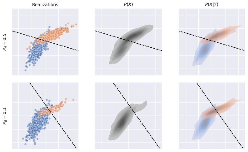
Figure 1: Example of prior probability shift generated with synthetic data using a normal distribution for each class. Scenario $A$ (1st row): original data distribution, in which the positive class (orange) and the negative class (blue) have the same prevalence, i.e., $p_{A}=0.5$. Scenario $B$ (2nd row): with respect to Scenario $A$ there is a shift in the prevalence such that $p_{B}=0.1$. Dashed lines represent linear hypotheses learnt from the corresponding empirical distributions. Note that, although the positive class and the negative class may have not changed in meaning between $A$ and $B$, i.e., $P_{A}(Y|X)=P_{B}(Y|X)$, the posteriors we would obtain by calibrating two soft classifiers trained from the two empirical distributions would likely differ. Note also that $P_{A}(X)\neq P_{B}(X)$ (2nd column) but $P_{A}(X|Y)=P_{B}(X|Y)$ (3rd column).

Prior probability shift is the type of shift which quantification methods have mostly been tested on, and the invariance assumption $P_{L}(X|Y)=P_{U}(X|Y)$ that is made in prior probability shift indeed guarantees that a number of quantification methods work well in these scenarios. In order to show this, let us take ACC as an example. The correction implemented in Equation 6 does not attempt to counter prior probability shift, but attempts to counter classifier bias (indeed, note that this correction is meaningful even in the absence of prior probability shift). This adjustment relies on Equation 4, which depends on two quantities, the tpr and the fpr of classifier $h$, that must be estimated on the training data $L$. Since $h(\mathbf{x})$ is the same for $L$ and $U$, the fact that $P_{L}(X|Y)=P_{U}(X|Y)$ (which is assumed to hold under probability shift) implies that $\hat{\operatorname{tpr}}_{h}=\operatorname{tpr}_{h}$ and $\hat{\operatorname{fpr}}_{h}=\operatorname{fpr}_{h}$. In other words, under prior probability shift ACC works well, since the assumption that the class-conditional distribution $P(X|Y)$ is invariant across $L$ and $U$ guarantees that our estimates of tpr and fpr are good estimates. Similar considerations apply to different quantification methods as well.

Prior probability shift has been widely studied in the quantification literature, both from a theoretical point of view (Tasche, 2017; Fernandes Vaz et al., 2019) and from an empirical point of view (Schumacher et al., 2021). Indeed, note that the artificial prevalence protocol (APP – see Section 2), on which most experimentation of quantification systems has been based, does nothing else than generate a set of samples characterised by prior probability shift with respect to the set from which they have been extracted; the APP recreates the $P_{L}(Y)\neq P_{U}(Y)$ condition by subsampling one of the two classes, and recreates the $P_{L}(X|Y)=P_{U}(X|Y)$ condition by performing this subsampling in a random fashion.

Most of the quantification literature is concerned with ways of devising robust estimators of class prevalence values in the presence of prior probability shift. Tasche (2017) proves that, when $P_{L}(Y)\neq P_{U}(Y)$ and $P_{L}(X|Y)=P_{U}(X|Y)$ (i.e., when we are in the presence of prior probability shift) the method ACC is Fisher-consistent, i.e., the error of ACC tends to zero when the size of the sample increases. Unfortunately, in practice, the condition of an unchanging $P(X|Y)$ is difficult to fulfil or verify.

At this point, it may be worth stressing that not every change in $P(Y)$ can be considered an instance of prior probability shift. Indeed, in Section 4.2 we present different cases of shift in the priors that are not instances of prior probability shift, and that we deem of particular interest for realistic applications of quantification.

4.2 Covariate Shift

Covariate shift (see Figure 3 for a graphical example) describes a situation in which (a) there is a change in the distribution $P(X)$ of the covariates (i.e., $P_{L}(X)\neq P_{U}(X)$), while (b) the distribution of the classes conditional on the covariates remains constant (i.e., $P_{L}(Y|X)=P_{U}(Y|X)$). In this type of shift, no further assumption is usually made as to whether the distribution $P(Y)$ of the classes and the class-conditional distribution $P(X|Y)$ change across $L$ and $U$.

In this paper, we are going to assume that also a change in the class-conditional distribution takes place, i.e., $P_{L}(X|Y)\neq P_{U}(X|Y)$. The rationale of this choice is that, without this assumption, there would be a possible overlap between the notion of prior probability shift and the notion of covariate shift. To see why, imagine a situation in which the positive and the negative examples are numerical univariate data each following a uniform distribution $\mathbf{U}(a,b)$ and $\mathbf{U}(c,d)$, with different parameters $a<b<c<d$. A change in the priors (i.e., $P_{L}(Y)\neq P_{U}(Y)$) would not cause any modification in the class-conditional distribution (i.e., $P_{L}(X|Y)=P_{U}(X|Y)$ would hold). Thus, by definition, this would squarely count as an example of prior probability shift, since these are the same conditions listed in Row 1 of Table 2. However, at the same time, the distribution of the covariates has also changed (i.e., $P_{L}(X)\neq P_{U}(X)$), since $P(X)=\mathbf{U}(a,b)P(Y=1)+\mathbf{U}(c,d)P(Y=0)$ and since the priors have changed, with the posterior distribution $P(Y|X)$ remaining stable across $L$ and $U$. Thus, this would also count as an example of covariate shift; see Figure 2 for a graphical explanation. For this reason, and for the sake of clarity in the exposition, in this work we will break the ambiguity by assuming that covariate shift implies that $P(X|Y)$ is not invariant across $L$ and $U$. As a final observation, note that the conditions of covariate shift are incompatible with a situation in which both $P(Y)$ and $P(X|Y)$ remain invariant. The reason is that $P(X)$ is assumed to change under the covariate shift assumptions, but, since $P(X)=P(X|Y=1)P(Y=1)+P(X|Y=0)P(Y=0)$, the only way in which this condition can hold true comes down to assuming either a change in $P(Y)$ or in $P(X|Y)$.

We will further distinguish between two types of covariate shift, i.e., (i) global covariate shift, in which the changes in the covariates occur globally, i.e., affect the entire population, and (ii) local covariate shift, in which the changes in the covariates occur locally, i.e., only affect certain subregions of the entire population. These two types of covariate shift will be the subject of Sections 4.2.1 and 4.2.2, respectively.

Figure 2: Possible overlap between the notions of prior probability shift and covariate shift, unless we assume that $P_{L}(X|Y)\neq P_{U}(X|Y)$ in covariate shift.

4.2.1 Global Covariate Shift

Global covariate shift occurs when there is an overall change in the representation function. We will study two variants of it that differ in terms of whether $P(Y)$ is invariant or not across $L$ and $U$: global pure covariate shift, in which $P_{L}(Y)=P_{U}(Y)$, and global mixed covariate shift, in which $P_{L}(Y)\neq P_{U}(Y)$ (the name “mixed” of course refers to the fact that there is a change in the distribution of the covariates and in the distribution of the labels). Both scenarios are interesting to test quantification methods on, but the latter is probably even more interesting, since changes in the priors are something that quantification methods are expected to be robust to.

Global pure covariate shift might occur when, for example, a sensor (in charge of generating the covariates) experiences a change (e.g., a partial damage, or a change in the lighting conditions for a camera); in this case, the prevalence values of the classes of interest do not change, but the measurements (covariates) might have been affected.

Global mixed covariate shift might occur when, for example, a quantifier is trained to monitor the proportion of positive opinions on a certain politician on Twitter on a daily basis and, after the quantifier has been deployed to production, there is a change in Twitter’s policy that allows for longer tweets. In this case, there is a variation in $P(X)$, since longer tweets become more likely; there is variation in $P(X|Y)$, since there will likely be longer positive tweets and longer negative tweets; $P(Y|X)$ will remain constant, since a change in the length of tweets does not make positive comments more likely or less likely; and $P(Y)$ can change too (because opinions on politicians do change in time), although not as a result of the change in tweet length.

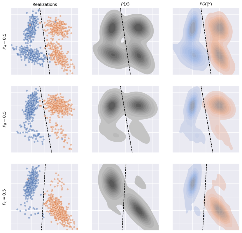
Figure 3: Example of global pure covariate shift generated with synthetic data using a normal distribution for each cluster. Situation $(a)$ (1st row): original data distribution. Each class consists on two clusters of data (for example positive or negative opinions of two different categories: Electronics and Books). Situation $(b)$ (2nd row): there is a shift in the number of opinions of one category, that affects both classes. $P(X)$ changes (see 2nd column) but $P(Y|X)$ remains invariant. Situation $C$ (3rd row), $P(X)$ changes abruptly, affecting the posterior probabilities $s(\mathbf{x})$ that a soft classifier, trained via induction on this scenario, would issue.

By taking into account the underlying conditions of pure covariate shift, it seems pretty clear that PCC (see Section 3.3) would represent the best possible choice. The reason is that PCC computes the estimate of the class prevalence values by relying on the posterior probabilities returned by a soft classifier $s$ (see Equation 7). Inasmuch as these posterior probabilities are reliable enough (i.e., when the soft classifier is well calibrated (Card and Smith, 2018)), the class prevalence values would be well estimated without further manipulations (i.e., there is no need to adjust for possible changes in the priors since, in the pure version, we assume $P(Y)$ has not changed); see Figure 3, 2nd row.

However, in practice, the posterior probabilities returned by $s$ might not align well with the underlying concept of the positive class (the soft classifier $s$ might not be well calibrated for the unlabelled distribution). This might be due to several reasons, but a relevant possibility is due to the inability of the learning device to find good parameters for the classifier. This might happen whenever the hypothesis (i.e., the soft classifier $s$) learnt by means of an inductive learning method (e.g., logistic regression) comes from an empirical distribution in which certain regions of the input space were insufficiently represented during training, and have later become more prevalent during test as a result of a change in $P(X)$; see Figure 2, 3rd row. This situation is certainly problematic, and would lead to a deterioration in performance of most aggregative quantifiers (including PCC). An in-depth theoretical analysis of the implications of pure covariate shift is offered by Tasche (2022), in which the author concludes that in order for PCC to prove resilient to covariate shift, the test distribution should be absolutely continuous with respect to the training distribution. This assumption also restricts the amount of divergence between training and test samples distributions. However, these are theoretical considerations that are hard (if not impossible) to verify in practice.

4.2.2 Local Covariate Shift

Consider a binary problem in which the positive class is a mixture of two (differently parameterised) Gaussians $\mathcal{N}_{1}$ and $\mathcal{N}_{2}$, i.e., that $P(X|Y=1)=\alpha\mathcal{N}_{1}+(1-\alpha)\mathcal{N}_{2}$. Assume there are analogous Gaussians $\mathcal{N}_{3}$ and $\mathcal{N}_{4}$ governing the distribution of negatives; see Figure 4. Assume now that there is a change (say, an increase) in the prevalence of datapoints from $\mathcal{N}_{1}$ leading to an overall change in the priors $P(Y)$. Note that this also implies an overall change in $P(X)$. There is also a change in $P(X|Y=1)$ (therefore, in $P(X|Y)$) since the parameter $\alpha$ of the mixture has changed (it is now more likely to find positive examples from $\mathcal{N}_{1}$). However, the change in the covariates is asymmetric, i.e., $P(X|Y=0)$ has not changed.

Situations like this naturally occur in real scenarios of interest for quantification. For example, in ecological modelling, researchers might be interested in estimating the prevalence of, e.g., different species of plankton in the sea. To do so, they analyse pictures of water samples taken by an automatic optical device, identify individual examplars of plankton, and estimate the prevalence of the different species via a quantifier (González et al., 2019). However, these plankton species are typically grouped, because of their high number, into coarse-grained superclasses (i.e., parent nodes from a taxonomy of classes), which means that no prevalence estimation for the subclasss is attempted. An increase in the prevalence value of one of the (super-)classes is often the consequence of an increase in the prevalence value of only one of its (hidden) subclasses. A similar example may be found in seabed cover mapping for coral reef monitoring (Beijbom et al., 2015); here, ecologists are interested in quantifying the presence of different species in images, often grouping the coral species and algae species into coarser-grained classes.

In contrast to global covariate shift, local covariate shift does not occur due to a variation in the feature representation function (e.g., an alteration of the device in charge of taking measurements, which would impact on the covariates) but due to changes in the priors of (sub-)classes that remain hidden. The most important implication for quantification concerns the fact that this shift would reduce to prior probability shift if the subclasses (the original species in our examples) were observed in place of the superclasses. We will only consider the case in which $P(Y)$ changes, since it is hard to think of any realistic scenario for asymmetric covariate shift in which the class prevalence values remain unaltered. Note also that, in extreme cases, an abrupt change in $P(Y)$ can end up compromising the condition $P_{L}(Y|X)=P_{U}(Y|X)$, for the same reasons why $P(Y|X)$ is altered in prior probability shift. However, under mild conditions, we can assume $P(Y|X)$ does not change, or does not change significantly.

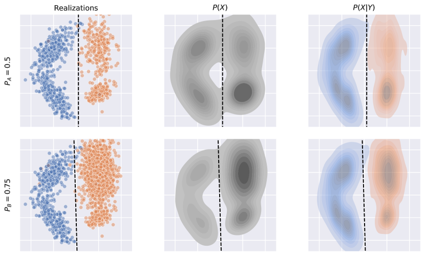
Figure 4: Example of local covariate shift generated with synthetic data using a normal distribution for each cluster. Situation (a) (1st row): original data distribution with two positive (orange) Gaussians $\mathcal{N}_{1}$, $\mathcal{N}_{2}$ and two negative (blue) Gaussians $\mathcal{N}_{3}$, $\mathcal{N}_{4}$. Situation (b) (2nd row): the prevalence of $\mathcal{N}_{1}$ grows.

4.3 Concept Shift

Concept shift arises when the boundaries of the classes change, i.e., when the underlying concepts of interest change across the training and the testing conditions. Concept shift is characterised by a change in the class-conditional distribution $P_{L}(X|Y)\neq P_{U}(X|Y)$, as well as a change in the posterior distribution $P_{L}(Y|X)\neq P_{U}(Y|X)$. Another way of saying this is that there is a change in the functional relationship between the covariates and the class labels; see Figure 5.

Figure 5 depicts a situation in which each of the two classes (say, documents relevant and non relevant, respectively, to a certain user information need) subsumes two subclasses, and one of the subclasses “switches class”, i.e., the documents contained in the subclass were once considered relevant to the information need and are now not relevant any more. Yet another example along these lines could be due to a change in the sensitivity of a response variable. So, for example, a change in the threshold above which the value of a continuous response variable indicates a positive example, is a change in the concept of “being positive”, which implies (i) a change in $P(Y|X)$, since some among the positive examples have now become negative, (ii) a change in $P(X|Y)$, since the positive and negative classes are inevitably distributed differently, and (iii) even a change in $P(Y)$, since the higher the threshold, the fewer the positive examples; however, the above does not imply any change in the marginal distribution $P(X)$.

There are other examples of concept shift which may, instead, lead to a change in $P(X)$ as well. Take, for example, the case of epidemiology (one of the quintessential applications of quantification) in which the spread of a disease (e.g., by a viral infection) is now manifested in the population by means of different symptoms (the covariates) due to a change in the pathogenic source (e.g., a mutation). In this paper, though, we will only be considering instances of concept shift in which the marginal distribution $P(X)$ does not change, since otherwise none of the four distributions of interest ($P(X)$, $P(Y)$, $P(X|Y)$, $P(Y|X)$) would be invariant across $L$ and $U$, which would make the problem essentially unlearnable.

Needless to say, concept shift represents the hardest type of shift for any quantification system (and, more in general, for any inductive inference model), since changes in the concept being modelled are external to the learning procedure, and since there is no possibility of behaving robustly to arbitrary changes in the functional relationship between the covariates and the labels. Attempts to tackle concept shift should inevitably entail a later phase of learning (as in continuous learning) in which the model is informed, possibly by means of new labelled examples, of the changes in the functional relationship between covariates and classes. To date, we are unaware of the existence of quantification methods devised to counter concept shift.

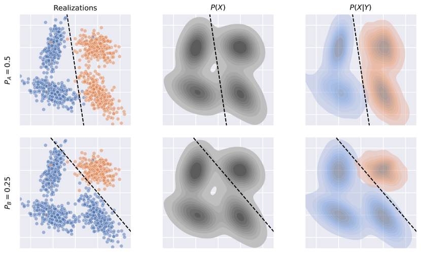
Figure 5: Example of concept shift generated with synthetic data using a normal distribution for each cluster. Situation (a) (1st row): original data distribution. Situation (b) (2nd row): the concept “negative” (blue) has changed in a way that it now encompasses one of the originally “positive” (orange) clusters, thus implying a change in $P(X|Y)$ and in $P(Y|X)$ but not in $P(X)$ (2nd column).

4.4 Recapitulation

In light of the considerations above, in Table 2 we present the specific types of shift that we consider in this paper. Concretely, this comes down to exploring plausible ways of filling out the blank cells of Table 1, which are indicated in grey in Table 2.

	$P(X)$	$P(Y)$	$P(X|Y)$	$P(Y|X)$	Definition	Experiments
Prior probability shift	$\neq$	$\neq$	=	$\neq$	§4.1	§5.3
Global pure covariate shift	$\neq$	=	$\neq$	=	§4.2.1	§5.4
Global mixed covariate shift	$\neq$	$\neq$	$\neq$	=	§4.2.1	§5.4
Local covariate shift	$\neq$	$\neq$	$\neq$	∗=∗	§4.2.2	§5.5
Concept shift	=	$\neq$	$\neq$	$\neq$	§4.3	§5.6

Table 2: The types of shift we consider. Greyed-out cells indicate assumptions we make (and that we discuss and justify in Section 4). Symbol * indicates a condition that can get compromised in extreme situations.

5 Experiments

In this section we describe experiments that we have carried out in which we simulate the different types of dataset shift described in the previous sections. For simplicity, we have simulated all these types of shift by using the same base datasets, which we describe in the following section.

5.1 Datasets

We extract the datasets we use for the experiments from a large crawl of 233.1M Amazon product reviews made available by McAuley et al. (2015); we use different datasets for simulating different types of shift. In order to extract these datasets from this crawl we first remove (a) all product reviews shorter than 200 characters and (b) all product reviews that have not been recognised as “useful” by any users. We concentrate our attention on two merchandise categories, Books and Electronics, since these are the two most populated categories in the corpus; in the next sections these two categories will sometimes be referred to as category $A$ and category $B$.

Every review comes with a (true) label, consisting of the number of stars (according to a “5-star rating”, with 1 star standing for “poor” and 5 stars standing for “excellent”) that the author herself has attributed to the product being reviewed. Note that the classes are ordered, and thus we can define $\mathcal{Y}_{\star}=\{s_{1},s_{2},s_{3},s_{4},s_{5}\}$, with $s_{i}$ meaning “$i$ stars”, and $s_{1}\prec s_{2}\prec s_{3}\prec s_{4}\prec s_{5}$. Since we deal with binary quantification, we exploit this order to generate, at desired “cut points” (i.e., thresholds below which a review is considered negative and above which is considered positive), binary versions of the dataset. We thus define the function “$\operatorname{binarise\_dataset}$”, that takes a dataset labelled according to $\mathcal{Y}_{\star}$ and a cut point $c$, and returns a new version of the dataset labelled according to a binary codeframe $\mathcal{Y}=\{0,1\}$; here, every labelled datapoint $(\mathbf{x},s_{i})$, with $s_{i}\in\mathcal{Y}_{\star}$, is converted into a datapoint $(\mathbf{x},y)$, with $y\in\mathcal{Y}$, such that $y=1$ (the positive class) if $i>c$, or $y=0$ (the negative class) if $i<c$; note that we filter out datapoints for which $i=c$. In the cases in which we want to retain all datapoints labelled with all possible numbers of stars, we simply specify $c$ as a real value intermediate between two integers (e.g., $c=2.5$).

	instances	$\filledstar\smallstar\smallstar\smallstar\smallstar$	$\filledstar\filledstar\smallstar\smallstar\smallstar$	$\filledstar\filledstar\filledstar\smallstar\smallstar$	$\filledstar\filledstar\filledstar\filledstar\smallstar$	$\filledstar\filledstar\filledstar\filledstar\filledstar$
Books	7,813,813	0.093	0.071	0.094	0.160	0.582
Electronics	1,889,965	0.193	0.079	0.093	0.178	0.457

Table 3: Dataset information for categories Books and Electronics, along with the prevalence for each different star rating.

5.2 General Experimental Setup

In all the experiments carried out in this study we fix the size of the training set to 5,000 and the size of each test sample to 500. For a given experiment we evaluate all quantification methods with the same test samples, but different experiments may involve different samples depending on the type of shift being simulated. We run different experiments, each targeting a specific type of dataset shift; within each experiment we simulate the presence, in a systematic and controlled manner, of different degrees of shift. When testing with different degrees of a given type of shift, for every such degree we randomly generate 50 test samples. In order to account for stochastic fluctuations in the results due to the random selection of a particular training set, we repeat each experiment 10 times. We carry out all the experiments by using the QuaPy open-source quantification library (Moreo et al., 2021). All the code for reproducing our experiments is available from a dedicated GitHub repository.

In order to turn raw documents into vectors, as the features we use tfidf-weighted words; we compute idf independently for each experiment by only taking into account the 5,000 training documents selected for that experiment. We only retain the words appearing at least 3 times in the training set, meaning that the number of different words (hence, the number of dimensions in the vector space) can vary across experiments.

As the evaluation measure we use absolute error (AE), since it is one of the most satisfactory (see (Sebastiani, 2020) for a discussion) and frequently used measures in quantification experiments, and since it is very easily interpretable. In the binary case, AE is defined as

$$\operatorname{AE}(p_{\sigma},\hat{p}_{\sigma})=|p_{\sigma}-\hat{p}_{\sigma}|$$ (9)

For each experiment we report the mean absolute error (MAE), where the mean is computed across all the samples with the same degree of shift and all the repetitions thereof. We perform statistical significance tests at different confidence levels in order to check for the differences in performance between the best method (highlighted in boldface in all tables) and all other competing methods. All methods whose scores are not statistically significantly different from the best one, according to a Wilcoxon signed-rank test on paired samples, are marked with a special symbol. We use superscript ${\dagger}$ to indicate that $0.001<$ p-value $<0.05$ (loosely speaking, that the scores are “somewhat similar”), while superscript ${\ddagger}$ indicates that $0.05\leq$ p-value (loosely speaking, that the scores are “very similar”); the absence of any such symbol thus indicates that p-value $\leq 0.001$ (loosely speaking, that the scores are “fairly different”).

All the quantification methods considered in this study are of the aggregative type and are described in Section 3.3. In addition to these methods, we had initially also considered the Sample Mean Matching (SMM) method (Hassan et al., 2020), but we removed this method from the experiments as we found it to be equivalent to the PACC method (we give a formal proof of this equivalence in Appendix A).

For the sake of fairness, underlying all quantification methods we use the same type of classifier. (All the quantification methods we use are aggregative, so all of them use an underlying classifier.) As our classifier of choice we use logistic regression, since it is a well-known classifier which also delivers “soft” predictions and is known to deliver reasonably well-calibrated posterior probabilities (these two characteristics are required for PCC, PACC, DyS, and SLD). We optimise the hyperparameters of the quantifier following Moreo and Sebastiani (2021), i.e., minimising a quantification-oriented loss function (here: MAE) via a quantification-oriented parameter optimisation protocol; we explore the values $C\in\{0.1,1,10,100,100\}$ (where $C$ is the inverse of the regularization strength), and the values class_weight $\in$ $\{\operatorname{Balanced}$, $\operatorname{None}\}$ (where class_weight indicates the relative importance of each class), via grid search. We evaluate each configuration of hyperparameters in terms of MAE over artificially generated samples using a held-out stratified validation set consisting of 40% of the training documents. This means that we optimise each classifier specifically for each quantifier, and the parameters we choose are the ones that best suit this particular quantifier. Once we have chosen the optimal values for the hyperparameters, we retrain the quantifier using the entire training set.

The quantification methods used in this study do not have any additional hyperparameters, except for DyS that has two, i.e., (i) the number of bins used to build the histograms and (ii) the distance function. In this work we fix these values to (i) 10 bins and (ii) the Topsoe distance, since these are the values that gave the best results in the work that originally introduced DyS (Maletzke et al., 2019).

5.3 Prior Probability Shift

5.3.1 Evaluation Protocol

For generating prior probability shift we consider all the reviews from categories Electronics and Books. Algorithm 1 describes the experimental setup for this type of shift. For binarising the dataset we follow the approach described in Section 5.1, using a cut point of $3$. We sample 5,000 training documents from the dataset using prevalence values of the positive class with values ranging from $0$ to $1$, at steps of $0.1$. (Since it is not possible to generate a classifier with no positive examples or no negative examples, we actually replace $p_{L}=0$ and $p_{L}=1$ with $p_{L}=0.02$ and $p_{L}=0.98$, respectively.) We draw test samples from the dataset varying, here too, the prevalence of the positive class using values in $\{0.0,0.1,..,0.9,1.0\}$. In order to give a quantitative indication of the degree of prior probability shift in each experiment, we compute the signed difference $(p_{L}-p_{U})$ rounded to one decimal, resulting in a real value in the range $[-1,1]$; to this respect, note that negative degrees of shift do not indicate an absence of shift, but indicate a presence of shift in which $p_{U}$ is greater than $p_{L}$ (for positive degrees, $p_{U}$ is lower than $p_{L}$).

For this experiment the number of test samples used for evaluation amounts to $11\times 11\times 50\times 10$ = 60,500 for each quantification algorithm we test.

Input: Datasets $A$ and $B$; Quantification learner $Q$

1:$D\leftarrow A\cup B$

2:$D\leftarrow\operatorname{binarise\_dataset}(D,\operatorname{cut\_point}=3)$

3:$\mathcal{L},\;\mathcal{U}\leftarrow\operatorname{split\_stratified(D)}$

4:for 10 repetitions do

5:     for $p^{L}\in\{0.02,0.1,0.2,...,0.8,0.9,0.98\}$ do

6:         /* Generate a sample from $\mathcal{L}$ with prevalence $p^{L}$ */

7:         $L\sim\mathcal{L}$ with $p_{L}=p^{L}$ and $|L|=5000$

8:         /* Use algorithm $Q$ to learn a quantifier $q$ on $L$ */

9:         $q\leftarrow Q.fit(L)$

10:         for 50 repetitions do

11:              /* Generating test samples */

12:              for $p^{U}\in\{0.0,0.1,...,0.9,1.0\}$ do

13:                  $U\sim\mathcal{U}$ with $p_{U}=p^{U}$ and $|U|=500$

14:                  $\hat{p}_{U}^{q}\leftarrow q.\operatorname{quantify}(U)$

15:                  $error\leftarrow\operatorname{AE}(p_{U},\hat{p}_{U}^{q})$                             

Algorithm 1 Protocol for generating prior probability shift.

5.3.2 Results

Table 4 and Figure 6 present the results of the prior probability shift experiments in the form of boxplots (blue boxes), where the outliers are indicated by black dots. In this case the SLD method stands out as the best performer, closely followed by DyS and PACC. These methods perform very well when the degree of shift is moderate, while their performance degrades as this degree increases. On the other hand, CC and PCC are clearly the worst performers; the reason is that, as stated previously, CC and PCC naturally inherit the bias of the underlying classifier, so when the divergence between the distribution they are biased towards (i.e., the training distribution) and the test distribution increases, their performance tends to decrease. These results are in line with previous studies in the quantification literature (e.g., (Maletzke et al., 2019; Schumacher et al., 2021; Moreo et al., 2021; Moreo and Sebastiani, 2022)), most of which has indeed focused on prior probability shift.

	CC	ACC	PCC	PACC	DyS	SLD
-1.0	.737	.000	.548	.001	.063	.001
-0.9	.479	.049	.439	.044	‡.053	.041
-0.8	.355	.088	.352	.077	.045	.049
-0.7	.271	.099	.278	.069	.040	‡.041
-0.6	.213	.094	.216	.054	.032	†.034
-0.5	.166	.086	.162	.042	.028	‡.029
-0.4	.126	.071	.115	.031	†.024	.023
-0.3	.091	.055	.093	.025	.021	.020
-0.2	.064	.041	.085	.023	.019	.017
-0.1	.047	.032	.091	.022	.017	.015
0.0	.035	.026	.111	.017	.016	.014
0.1	.048	.034	.090	.021	.018	.017
0.2	.064	.046	.084	.023	†.019	.018
0.3	.092	.063	.089	.025	.022	.020
0.4	.127	.077	.112	.029	.026	.022
0.5	.167	.089	.160	.036	.030	.024
0.6	.213	.096	.213	.045	.035	.025
0.7	.272	.095	.276	.053	.043	.027
0.8	.355	.081	.351	.058	.053	.030
0.9	.478	.052	.440	.039	.062	.029
1.0	.742	.020	.551	.002	.076	.016

Table 4: Results for prior probability shift experiments in terms of $\operatorname{MAE}$. Each row corresponds to a given degree of shift, measured as $(p_{U}-p_{L})$ (rounded to one decimal).

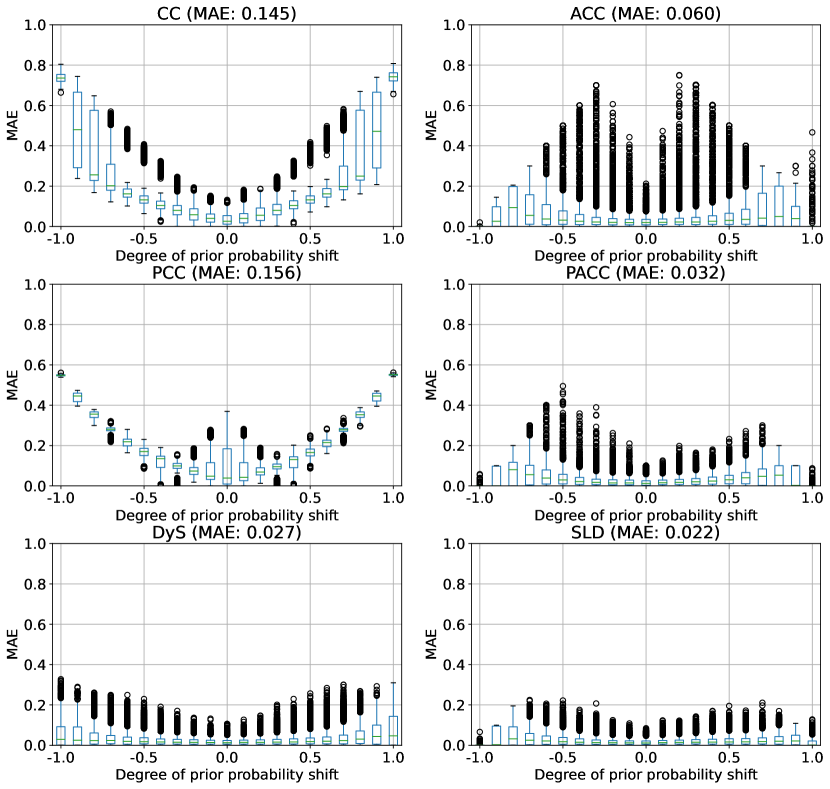
Figure 6: Results obtained for prior probability shift; the error measure is MAE and the degree of shift is computed as $(p_{U}-p_{L})$ (rounded to one decimal).

One interesting observation that emerges from Figure 6 has to do with the stability of the methods. ACC shows a tendency to sporadically yield anomalously high levels of error. Those levels of error correspond to cases in which the training sample is severely imbalanced ($p_{L}=0.02$ or $p_{L}=0.98$). Note that, the correction implemented by Equation 4 may turn unreliable when the estimation of $\operatorname{tpr}$ itself is unreliable (this is likely to occur when the amount of positives is 2%, i.e., when $p_{L}=0.02$) and/or when the estimation of $\operatorname{fpr}$ is unreliable (this is likely to occur when the amount of negatives is 2%, i.e., when $p_{L}=0.98$). Yet another cause might include the instability of the denominator (this happens when $\operatorname{tpr}\approx\operatorname{fpr}$), which could, in turn, require clipping the output in the range $[0,1]$. After analyzing the 100 worst cases, we verified that in 36% of the cases involved clipping, in 46% of the cases the denominator turned out to be smaller than 0.05.

Note that, if these extreme cases were to be removed, the average scores obtained by ACC would not substantially differ from those obtained by other quantification methods such as PACC or DyS.

5.4 Global Covariate Shift

5.4.1 Evaluation Protocol

For generating global covariate shift, we modify the ratio between the documents in category $A$ (Books) and those in category $B$ (Electronics), across the training data and the test samples. We binarise the dataset at a cut point of 3, as described in Section 5.1. We vary the prevalence $\alpha$ of category $A$ (the prevalence of category $B$ is $(1-\alpha)$), in the training data ($\alpha^{L}$) and in the test samples ($\alpha^{U}$), in the range $[0,1]$ with steps of 0.1, thus giving rise to 121 possible combinations. For the sake of a clear exposition, we present the results for different degrees of global covariate shift, measured as the signed difference between $\alpha^{L}$ and $\alpha^{U}$, resulting in a real value in the range $[-1,+1]$. We vary the priors of the positive class using the values $\{0.25,0.50,0.75\}$ in both the training data and the test samples, in order to simulate cases of global pure covariate shift, where $P_{L}(Y)=P_{U}(Y)$, and global mixed covariate shift, where $P_{L}(Y)\neq P_{U}(Y)$. Note that even if the global pure covariate shift scenario is particularly awkward for a quantification setting (since the prevalence of the positive class in the training data coincides with the one in the test data), it is interesting because it shows how quantifiers react just to a mere change in the covariates. Algorithm 2 describes the experimental setup for this type of shift.

For this experiment the number of test samples used for evaluation amounts to $3\times 3\times 11\times 11\times 50\times 10$ = 544,500 for each quantification algorithm we test.

Input: Datasets $A$ and $B$; Quantification algorithm $Q$

1:$A\leftarrow\operatorname{binarise\_dataset}(A,\operatorname{cut\_point=3})$

2:$B\leftarrow\operatorname{binarise\_dataset}(B,\operatorname{cut\_point=3})$

3:$\mathcal{L}_{A},\mathcal{U}_{A}\leftarrow\operatorname{split\_stratified}(A)$

4:$\mathcal{L}_{B},\mathcal{U}_{B}\leftarrow\operatorname{split\_stratified}(B)$

5:for 10 repetitions do

6:     for $p^{L}\in\{0.25,0.50,0.75\}$ do

7:         for $\alpha^{L}\in\{0.0,0.1,...,0.9,1.0\}$ do

8:              /* Generate a training sample $L$ from $\mathcal{L}_{A}$ and $\mathcal{L}_{B}$ with prevalence $p^{L}$

9:                 and a proportion $\alpha^{L}$ of documents from $\mathcal{L}_{A}$ */

10:              $L_{A}\sim\mathcal{L}_{A}$ with $p_{L_{A}}=p^{L}$ and $|L_{A}|=\lceil\alpha^{L}\cdot 5000\rceil$

11:              $L_{B}\sim\mathcal{L}_{B}$ with $p_{L_{B}}=p^{L}$ and $|L_{B}|=\lfloor(1-\alpha^{L})\cdot 5000\rfloor$

12:              $L\leftarrow L_{A}\cup L_{B}$

13:              /* Use quantification algorithm $Q$ to learn a quantifier $q$ on $L$ */

14:              $q\leftarrow Q.fit(L)$

15:              for 50 repetitions do

16:                  /* Generating test samples */

17:                  for $p^{U}\in\{0.25,0.50,0.75\}$ do

18:                       for $\alpha^{U}\in\{0.0,0.1,...,0.9,1.0\}$ do

19:                           $U_{A}\sim\mathcal{U}_{A}$ with $p_{U_{A}}=p^{U}$ and $|U_{A}|=\lceil\alpha^{U}\cdot 500\rceil$

20:                           $U_{B}\sim\mathcal{U}_{B}$ with $p_{U_{B}}=p^{U}$ and $|U_{B}|=\lfloor(1-\alpha^{U})\cdot 500\rfloor$

21:                           $U\leftarrow U_{A}\cup U_{B}$

22:                           $\hat{p}_{U}^{q}\leftarrow q.\operatorname{quantify}(U)$

23:                           $error\leftarrow AE(p_{U},\hat{p}_{U}^{q})$                                                                      

Algorithm 2 Protocol for generating global covariate shift.

5.4.2 Results

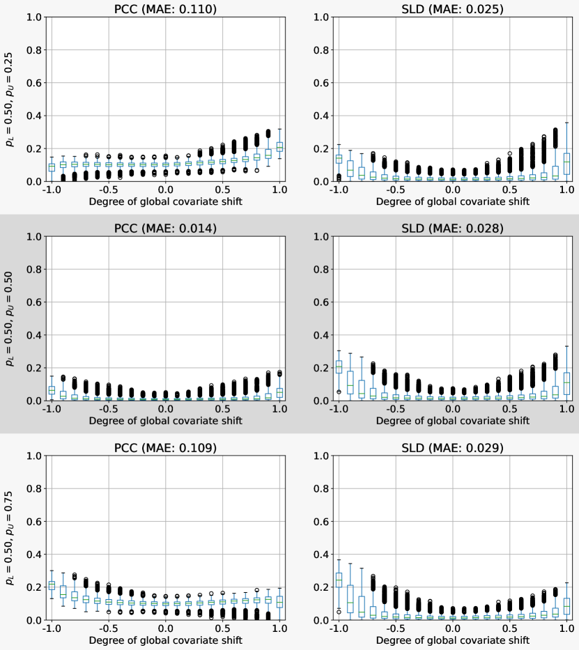
Figure 7: Results for global covariate shift with $p_{L}=0.5$. The error measure is MAE and the degree of covariate shift is computed as $(\alpha^{L}-\alpha^{U})$. Figures with a grey background represent cases of global pure covariate shift, in which $P_{L}(Y)=P_{U}(Y)$.

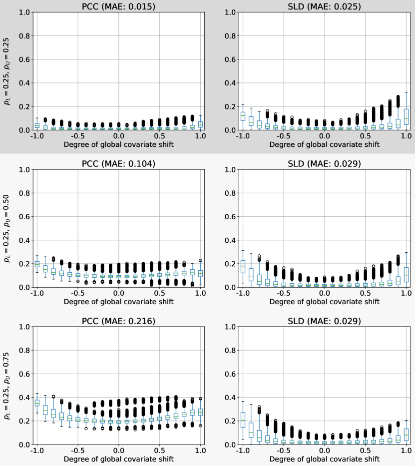
Figure 8: Results for global covariate shift with $p_{L}=0.25$. Error measure is MAE and the degree of covariate shift is computed as $(\alpha^{L}-\alpha^{U})$. Figures with a grey background represent cases of global pure covariate shift, in which $P_{L}(Y)=P_{U}(Y)$.

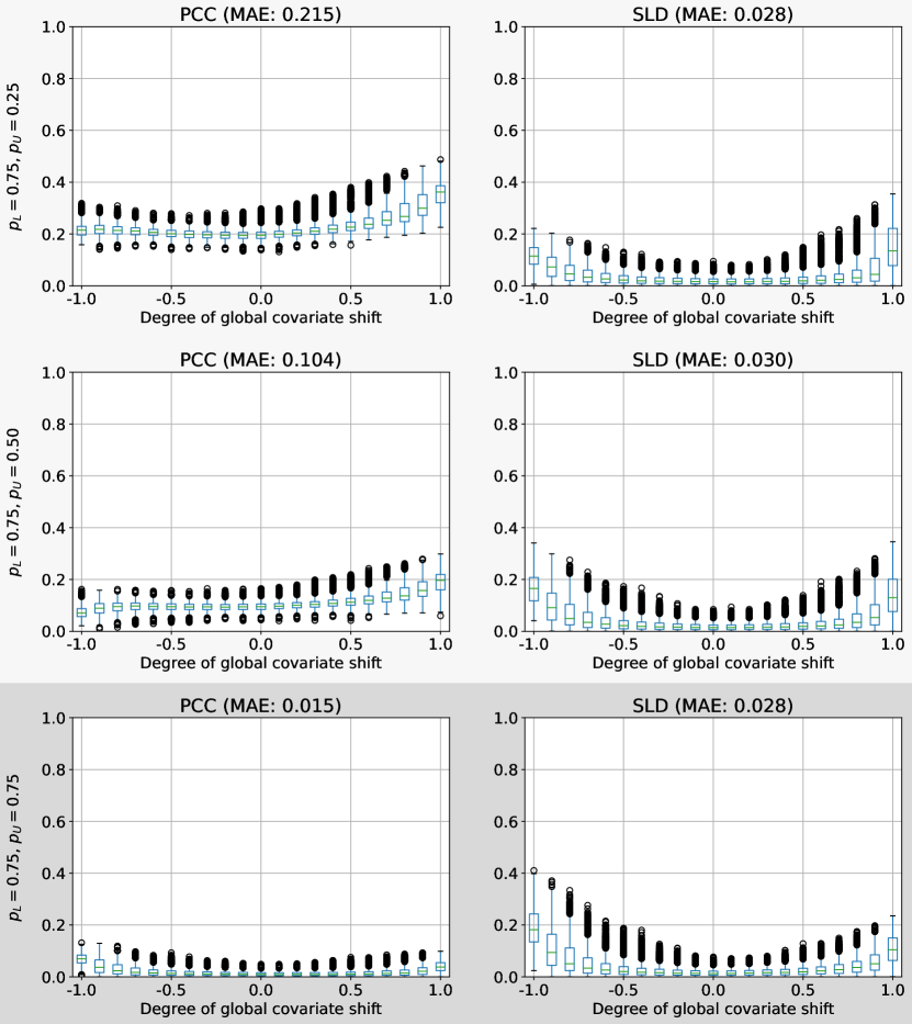
Figure 9: Results for global covariate shift with $p_{L}=0.75$. Error measure is MAE and the degree of covariate shift is computed as $(\alpha^{L}-\alpha^{U})$. Figures with a grey background represent cases of global pure covariate shift, in which $P_{L}(Y)=P_{U}(Y)$.

We now report the results for the scenario in which the data exhibits global pure covariate shift (see Tables 5, 6, 7, where global pure covariate shift is represented by the columns with a grey background, and Figures 7, 8, 9). As can be expected, the bigger the degree of such shift, the worse the performance of the methods. Note that a degree of global pure covariate shift equal to 1 (resp., -1) means that the system was trained with documents only from category $A$ (resp., $B$) while the testing samples only have documents from category $B$ (resp., $A$). On the other hand, low degrees of global pure covariate shift represent the situation in which similar values of $\alpha^{L}$ and $\alpha_{U}$ were used. The experiments show that the method most robust to global pure covariate shift is PCC, which is consistent with the theoretical results of Tasche (2022). PCC is able to provide good results, beating the other methods consistently, even when the degree of global pure covariate shift is high. On the other hand, methods like SLD, that show excellent performance under prior probability shift, perform poorly under high values of global pure covariate shift.

	$p_{U}=0.25$						$p_{U}=0.5$						$p_{U}=0.75$
	CC	ACC	PCC	PACC	DyS	SLD	CC	ACC	PCC	PACC	DyS	SLD	CC	ACC	PCC	PACC	DyS	SLD
-1.0	.029	.069	.085	.044	.080	.133	.107	.147	.065	.109	.142	.200	.231	.225	.213	‡.190	.188	.236
-0.9	.052	.046	.098	.033	.052	.078	.061	.083	.037	.064	.084	.110	.166	.132	.169	‡.114	.112	.128
-0.8	.060	.034	.101	.025	.037	.052	.042	.057	.025	.043	.055	.071	.137	.090	.145	†.076	.074	.082
-0.7	.065	.029	.102	.023	.031	.039	.033	.044	.020	.035	.043	.051	.117	.064	.130	‡.054	.053	‡.055
-0.6	.068	.025	.103	.021	.025	.030	.025	.034	.015	.027	.033	.037	.103	.047	.120	.039	‡.039	‡.040
-0.5	.070	.022	.101	.020	.022	.024	.021	.029	.014	.024	.028	.030	.093	.038	.113	.032	.032	.031
-0.4	.072	†.021	.102	‡.020	.020	‡.020	.018	.025	.012	.021	.024	.025	.085	.032	.109	.029	.026	.025
-0.3	.074	.020	.101	.020	‡.019	.018	.016	.023	.011	.019	.021	.021	.080	.027	.105	.025	.022	.021
-0.2	.074	.019	.101	.019	.018	.016	.015	.020	.010	.017	.019	.018	.075	.023	.102	.022	.020	.018
-0.1	.076	.019	.101	.019	.017	.015	.014	.019	.010	.017	.018	.016	.072	.021	.100	.020	.018	.016
0.0	.077	.018	.102	.017	.017	.015	.014	.018	.009	.016	.017	.015	.068	.019	.098	.018	.017	.015
0.1	.080	.019	.104	.017	.018	.015	.014	.019	.010	.016	.018	.016	.068	.019	.099	.019	.018	.016
0.2	.084	.022	.108	.020	.020	.016	.015	.020	.011	.018	.020	.017	.068	.020	.100	.019	.019	.017
0.3	.087	.025	.112	.023	.024	.017	.016	.021	.011	.019	.023	.019	.069	.020	.102	.019	.020	‡.019
0.4	.092	.030	.117	.028	.028	.020	.018	.023	.012	.020	.026	.021	.070	.021	.105	.020	.022	†.021
0.5	.097	.035	.122	.035	.033	.023	.019	.025	.013	.022	.030	.023	.073	‡.022	.108	.022	.025	‡.022
0.6	.105	.044	.130	.045	.042	.027	.022	.028	.015	.025	.037	.027	.075	.025	.112	.026	.030	‡.026
0.7	.114	.056	.139	.060	.053	.034	.025	.032	.018	.029	.046	.033	.077	.028	.114	.032	.036	.030
0.8	.127	.075	.152	.082	.074	.044	.031	.040	.022	.036	.061	.044	.078	.033	.117	.041	.046	.039
0.9	.148	.105	.170	.115	.112	.063	.040	.052	.030	.047	.089	.061	.078	.041	.118	.052	.060	.050
1.0	.194	.168	.212	.183	.203	.124	.070	.090	.055	.087	.155	.115	.066	.053	.107	†.056	.093	.086

Table 5: Results for global covariate shift when $p_{L}=0.5$ in terms of MAE. Each row contains the results for a degree in covariate shift computed as $(\alpha^{L}-\alpha^{U})$. Results are presented in three groups, depending on the prevalence used for the positive class in the test samples $p_{U}$. Columns with a grey background represent cases of of global pure covariate shift, in which $P_{L}(Y)=P_{U}(Y)$.

	$p_{U}=0.25$						$p_{U}=0.5$						$p_{U}=0.75$
	CC	ACC	PCC	PACC	DyS	SLD	CC	ACC	PCC	PACC	DyS	SLD	CC	ACC	PCC	PACC	DyS	SLD
-1.0	.059	.083	.040	.067	.127	.115	.200	.175	.195	.160	.221	.174	.340	.267	.351	.253	.290	.207
-0.9	.035	.053	.024	.043	.081	.075	.145	.107	.158	.097	.138	.107	.265	.168	.296	.158	.180	.123
-0.8	.029	.038	.018	.032	.060	.050	.114	.070	.136	.063	.096	.068	.221	.111	.265	.103	.126	.080
-0.7	.025	.031	.016	.027	.044	.037	.096	.053	.122	.048	.069	‡.049	.195	.078	.242	.073	.090	.054
-0.6	.024	.026	.014	.022	.034	.029	.083	.041	.112	.038	.051	.035	.175	.058	.226	.056	.065	.038
-0.5	.023	.024	.013	.020	.028	.023	.075	.035	.106	.033	.041	.028	.163	.048	.215	.048	.051	.029
-0.4	.022	.023	.012	.019	.024	.019	.070	.032	.100	.030	.034	.024	.154	.042	.207	.045	.040	.024
-0.3	.022	.022	.012	.018	.022	.018	.065	.030	.098	.029	.028	.021	.146	.039	.203	.043	.033	.021
-0.2	.022	.021	.012	.017	.020	.016	.062	.027	.094	.026	.024	.019	.142	.034	.197	.039	.028	.018
-0.1	.021	.021	.012	.017	.018	.015	.061	.026	.093	.025	.021	.017	.140	.031	.195	.036	.023	.017
0.0	.021	.021	.013	.017	.017	.015	.060	.025	.092	.024	.020	.017	.138	.030	.193	.034	.021	.017
0.1	.022	.021	.013	.017	.018	.015	.061	.025	.094	.024	.020	.018	.140	.029	.197	.032	.022	.019
0.2	.022	.022	.013	.018	.019	.016	.063	.025	.096	.023	.021	.020	.144	.029	.201	.030	.024	.020
0.3	.022	.021	.014	.019	.020	.018	.067	.024	.098	.022	.024	.021	.151	.029	.207	.029	.027	.022
0.4	.022	.022	.015	.020	.023	.020	.072	.025	.102	.023	.028	.023	.160	.033	.214	.032	.033	.023
0.5	.022	.024	.016	.022	.026	.023	.079	.028	.107	.026	.034	.025	.171	.039	.224	.039	.039	.024
0.6	.023	.026	.016	.024	.031	.028	.085	.033	.112	.031	.040	.029	.182	.049	.235	.052	.048	.027
0.7	.026	.029	.019	.029	.038	.035	.090	.040	.118	.039	.051	.034	.195	.066	.248	.073	.061	.031
0.8	.030	.036	.022	.035	.048	.046	.098	.053	.121	.053	.067	.046	.209	.089	.256	.099	.081	.038
0.9	.036	.045	.030	.048	.066	.065	.104	.070	.127	.068	.088	.064	.223	.119	.272	.126	.103	.051
1.0	.057	.069	.049	.081	.099	.116	.090	.090	.118	.082	.108	.112	.218	.148	.275	.141	.110	.084

Table 6: Results for global covariate shift when $p_{L}=0.25$ in terms of MAE. Each row contains the results for a degree in covariate shift computed as $(\alpha^{L}-\alpha^{U})$. Results are presented in three groups, depending on the prevalence used for the positive class in the test samples $p_{U}$. Columns with a grey background represent cases of global pure covariate shift, in which $P_{L}(Y)=P_{U}(Y)$.

	$p_{U}=0.25$						$p_{U}=0.5$						$p_{U}=0.75$
	CC	ACC	PCC	PACC	DyS	SLD	CC	ACC	PCC	PACC	DyS	SLD	CC	ACC	PCC	PACC	DyS	SLD
-1.0	.171	.057	.218	.047	.070	.115	.054	.085	.075	‡.062	.116	.169	.074	.135	.067	.122	.160	.194
-0.9	.168	.046	.218	.036	.052	.075	.063	.054	.089	.040	.074	.100	.052	.083	.042	.076	.097	.111
-0.8	.165	.035	.215	.028	.040	.054	.066	.042	.094	.033	.052	.069	.041	.062	.031	.054	.066	.075
-0.7	.159	.032	.211	.028	.039	.042	.066	.035	.096	.029	.046	.050	.033	.046	.023	.040	.052	.052
-0.6	.154	‡.030	.207	.030	.035	.033	.065	.032	.096	.028	.038	.039	.030	.038	.019	.032	.040	.039
-0.5	.149	.032	.202	.033	.031	.028	.063	.031	.095	.027	.033	.031	.028	.033	.017	.028	.034	.031
-0.4	.146	.032	.199	.035	.029	.024	.062	.029	.094	.027	.029	.026	.026	.029	.015	.025	.029	.025
-0.3	.145	.032	.198	.035	.025	.022	.064	.029	.094	.026	.025	.023	.023	.026	.014	.022	.025	.021
-0.2	.144	.032	.195	.036	.023	.021	.064	.027	.094	.025	.022	.020	.022	.024	.012	.019	.021	.018
-0.1	.145	.030	.196	.033	.022	.019	.066	.025	.095	.023	.020	.018	.020	.022	.012	.018	.019	.016
0.0	.146	.028	.196	.030	.021	.019	.068	.024	.096	.022	.020	.017	.019	.020	.011	.016	.018	.015
0.1	.150	.027	.201	.028	.022	.018	.070	.023	.099	.021	.021	.017	.019	.019	.011	.016	.018	.016
0.2	.156	.030	.208	.029	.026	.019	.073	.025	.102	.022	.024	.018	.019	.020	.011	.017	.020	.017
0.3	.164	.034	.215	.033	.032	.020	.078	.026	.107	.024	.028	.019	.020	.020	.012	.017	.023	.018
0.4	.173	.043	.224	.042	.040	.021	.084	.030	.112	.028	.033	.022	.020	.021	.012	.018	.026	.021
0.5	.185	.054	.235	.054	.050	.025	.091	.036	.117	.033	.040	.025	.021	.023	.013	.019	.029	.023
0.6	.201	.071	.248	.073	.064	.030	.101	.045	.125	.042	.050	.029	.023	.025	.014	.021	.035	.028
0.7	.223	.097	.266	.102	.082	.037	.116	.060	.136	.057	.063	.037	.026	.030	.017	.024	.041	.034
0.8	.244	.130	.284	.139	.111	.050	.128	.078	.146	.076	.086	.050	.030	.035	.020	.029	.055	.044
0.9	.284	.178	.317	.186	.161	.074	.155	.106	.166	.102	.120	.074	.037	.043	.026	.035	.070	.060
1.0	.345	.255	.361	.265	.228	.149	.196	.158	.194	.153	.172	.140	.059	.069	.043	.059	.100	.106

Table 7: Results for global covariate shift when $p_{L}=0.75$ in terms of MAE. Each row contains the results for a degree in covariate shift computed as $(\alpha^{L}-\alpha^{U})$. Results are presented in three groups, depending on the prevalence used for the positive class in the test samples $p_{U}$. Columns with a grey background represent cases of global pure covariate shift, in which $P_{L}(Y)=P_{U}(Y)$.

The situation changes drastically when analysing the results for global mixed covariate shift (which in the tables are represented by the columns with a white background), i.e., when also $P(Y)$ changes across training data and test data. In these cases, the performance of methods like PCC or CC (methods that performed very well under the presence of global pure covariate shift) degrades, due to the fact that these methods do not attempt any adjustment to the prevalence of the test data. In this case, methods designed to deal with prior probability shift, such as SLD, stand as the best performers. This is interesting, since this experiment represents a situation in which a change in the covariates happens along with a change in the priors, thus harming the calibration of the posterior probabilities on which PCC rests upon.

5.5 Local Covariate Shift

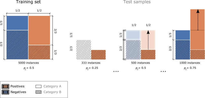
Figure 10: Conceptual diagram illustrating our local covariate shift protocol.

5.5.1 Evaluation Protocol

For simulating local covariate shift we generate a shift in the class conditional distribution of only one of the classes. In order to do so, categories $A$ and $B$ are treated as subclasses, or clusters, of the positive and negative classes. Figure 10 might help in understanding this protocol. The main idea is to alter the prevalence $P(Y)$ of the test samples by just changing the prevalence of positive documents of one of the subclasses (e.g., of category $A$) while maintaining the rest (e.g., positives and negatives in $B$ and the negatives of $A$) unchanged. Following this procedure, we let the class-conditional distribution of the positive examples $P(X|Y=1)$ vary, while the class-conditional distribution of the negative examples $P(X|Y=0)$ remains constant.

For this experiment, we keep the training prevalence fixed at $p_{L}=0.5$, while we vary the test prevalence $p_{U}$ artificially. To allow for a wider exploration of the range of the prevalence values $p_{U}$ that can be achieved by varying only the number of positives in category $A$, we start from a configuration in which $\frac{2}{3}$ of the positives in the training set are from category $A$ and the remaining $\frac{1}{3}$ are from category $B$. Both categories contribute to the training set with exactly the same number of documents (2,500 each, since the training set contains 5,000 documents, as before). The set of negative examples is composed of $\frac{1}{3}$ documents from $A$ and $\frac{2}{3}$ documents from $B$. In the test samples all these proportions are kept fixed except for the positive documents from category $A$, so that a desired prevalence value is reached by removing, or adding, positives of this category. Note that this process generates test samples of varying sizes. In particular, when the test size is equal to 500, the proportions of positive and negative documents, as well as the proportion of documents from $A$ and $B$, match the proportions used in the training set. Using this procedure we explore $p_{U}$ in the range $[0.25,0.75]$ at steps of 0.05 (see Algorithm 3).

For this experiment the number of test samples used for evaluation amounts to $11\times 11\times 50\times 10$ = 60,500 for each quantification algorithm we test.

Input: Datasets $A$ and $B$; Quantification algorithm $Q$

1:$A\leftarrow\operatorname{binarise\_dataset}(A,\operatorname{cut\_point=3})$

2:$B\leftarrow\operatorname{binarise\_dataset}(B,\operatorname{cut\_point=3})$

3:$\mathcal{L}_{A},\mathcal{U}_{A}\leftarrow\operatorname{split\_stratified}(A)$

4:$\mathcal{L}_{B},\mathcal{U}_{B}\leftarrow\operatorname{split\_stratified}(B)$

5:for 10 repetitions do

6:     $L_{A}\sim\mathcal{L}_{A}$ with $p_{L_{A}}=\frac{2}{3}$ and $|L_{A}|=2500$

7:     $L_{B}\sim\mathcal{L}_{B}$ with $p_{L_{B}}=\frac{1}{3}$ and $|L_{B}|=2500$

8:     $L\leftarrow L_{A}\cup L_{B}$      /* Note $p_{L}=\frac{1}{2}$ and $|L|=5000$ */

9:     /* Use quantification algorithm $Q$ to learn a quantifier $q$ on $L$ */

10:     $q\leftarrow Q.fit(L)$

11:     for 50 repetitions do

12:         $U^{\ominus}_{A}\sim\mathcal{U}_{A}$ with $p_{U^{\ominus}_{A}}=0$ and $|U^{\ominus}_{A}|=\frac{250}{3}$

13:         $U_{B}\sim\mathcal{U}_{B}$ with $p_{U_{B}}=\frac{1}{3}$ and $|U_{A}|=250$

14:         /* Note $p_{\{U^{\ominus}_{A}\cup U_{B}\}}=\frac{1}{4}$ */

15:         for $p_{U}\in\{0.25,0.3,0.35,\ldots,0.75\}$ do

16:              solve for $\operatorname{POS}$ the equation $p_{U}=\frac{\frac{250}{3}+\operatorname{POS}}{\frac{250}{3}+250+\operatorname{POS}}$

17:              $U^{\oplus}_{A}\sim\mathcal{U}_{A}$ with $p_{U^{\oplus}_{A}}=1$ and $|U^{\oplus}_{A}|=\operatorname{POS}$

18:              $U\leftarrow U^{\oplus}_{A}\cup U^{\ominus}_{A}\cup U_{B}$

19:              $\hat{p}_{U}^{q}\leftarrow q.\operatorname{quantify}(U)$

20:              $error\leftarrow AE(p_{U},\hat{p}_{U}^{q})$               

Algorithm 3 The protocol for generating local covariate shift.

5.5.2 Results

The results we have obtained for local covariate shift (orange boxes) are displayed in Figure 11. For easier comparison, this plot also shows results for the cases in which the class-conditional distributions are constant across the training data and the test data (blue boxes), i.e., when the type of shift is prior probability shift.

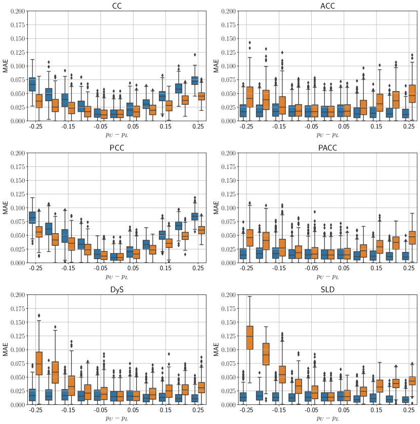
Figure 11: Results for local covariate shift expressed in terms of $\operatorname{MAE}$. Blue boxes represent the situation in which $P_{L}(X|Y)=P_{U}(X|Y)$ while orange boxes represent the situation in which $P_{L}(X|Y)\neq P_{U}(X|Y)$ because $P_{L}(X|Y=1)\neq P_{U}(X|Y=1)$. The degree of shift in the priors is shown along the x-axis and is computed as $(p_{U}-p_{L})$ rounded to two decimals.

Consistently with the results of Section 5.3.2, most quantification algorithms (except for CC and PCC) work reasonably well (see the blue boxes) when the class-conditional distributions are invariant across the training and the test data. Instead, when the class-conditional distributions change, the performance of these algorithms tends to degrade. This should come at no surprise given that all the adjustments implemented in the quantification methods we consider (as well as in all other methods we are aware of) rely on the assumption that the class-conditional distributions are invariant. The exception to this are CC and PCC, the only methods that do not attempt to adjust the priors. What comes instead as a surprise is not only that the performance of CC and PCC does not degrade, but that this performance seems to improve (i.e., the orange boxes in the extremes are systematically below the blue boxes for CC and PCC). This apparently strange behaviour can be explained as follows. When $p_{U}\ll p_{L}$, CC and PCC will naturally tend to overestimate the true prevalence. However, in this case, the positive examples in the test sample happen to mostly be from category $B$. Since the underlying classifier has been trained on a dataset in which the positives from category $A$ were more abundant ($\frac{2}{3}$) than the positives from category $B$ ($\frac{1}{3}$), the classifier has more problems in classifying positives from $B$ than from category $A$. This has the consequence that the overestimation brought about by CC and PCC is partially compensated (that is, positive examples from $B$ tend to be misclassified as negatives more often), and thus the final $\hat{p}_{U}$ gets closer to the real value $p_{U}$. On the other side, when $p_{U}\gg p_{L}$, CC and PCC will tend to underestimate $\hat{p}$. However, in this scenario positive examples mostly belong to category $A$, which the classifier identifies as positives more easily (since it has been trained on a relatively higher number of positives from $A$), thus increasing the value of $\hat{p}_{U}$ and making it closer to the actual value $p_{U}$.

A fundamental conclusion of this experiment is that, when the class-conditional distributions change, the adjustment implemented by the most sophisticated quantification methods can become detrimental. This is important since, in real applications, there is no guarantee that the type of shift a system is confronted with is prior probability shift, nor is there any general way for reliably identifying the type of shift involved. This experiment also shows how the bias inherited by CC and PCC can, under some circumstances, be “serendipitously” mitigated, at least in part. (We will see a similar example when studying concept shift in Section 5.6.)

5.6 Concept Shift

5.6.1 Evaluation Protocol

Input: Categories $A$ and $B$; Quantification algorithm $Q$

1:/* Sample $\mathcal{D}$ balanced with respect to number of stars */

2:$D\sim A\cup B$ with $p_{D}(\mathcal{Y}_{\star})=(0.2,0.2,0.2,0.2,0.2)$

3:$\mathcal{L},\;\mathcal{U}\leftarrow\operatorname{split\_stratified(\emph{D})}$

4:for 10 repetitions do

5:     for $c^{L}\in\{1.5,2.5,3.5,4.5\}$ do

6:         /* Generate a sample from $\mathcal{L}$ */

7:         $L\sim\mathcal{L}$ with $|L|=5000$

8:         /* Binarising using this specific cut point */

9:         $L\leftarrow\operatorname{binarise\_dataset}(L,\operatorname{cut\_point}=c^{L})$

10:         /* Use quantification algorithm $Q$ to learn $q$ on $L$ */

11:         $q\leftarrow Q.fit(L)$

12:         for 50 repetitions do

13:              /* Generating test samples */

14:              for $c^{U}\in\{1.5,2.5,3.5,4.5\}$ do

15:                  $U\sim\mathcal{U}$ with $|U|=500$

16:                  /* Binarising using this specific cut point */

17:                  $U\leftarrow\operatorname{binarise\_dataset}(U,\operatorname{cut\_point}=c^{U})$

18:                  $\hat{p}_{U}^{q}\leftarrow q.\operatorname{quantify}(U)$

19:                  $error\leftarrow AE(p_{U},\hat{p}_{U}^{q})$                             

Algorithm 4 Protocol for generating concept shift.

In order to simulate concept shift we exploit the ordinal nature of the original 5-star ratings. Specifically, we simulate changes in the concept of “being positive” by varying, in a controlled manner, the threshold above which a review is considered positive. The protocol we propose thus comes down to varying the cut points in the training set ($c^{L}$) and in the test set ($c^{U}$) independently, so that the notion of what is considered positive differs between the two sets. For example, by imposing a training cut point of $c^{L}=1.5$ we are mapping 1-star to the negative class, and 2-, 3-, 4-, and 5-stars to the positive class. In other words, everything but strongly negative reviews are considered positive in the training set. If, at the same time, we set the test cut point at $c^{U}=4.5$, we are generating a large shift in the concept of “being positive”, since in the test set only strongly positive reviews (5 stars) will be considered positive. For 5 classes there are 4 possible cut points $\{1.5,2.5,3.5,4.5\}$; the protocol explores all combinations systematically (see Algorithm 4).

We use the signed difference $(c^{L}-c^{U})$ as an indication of the degree of concept shift, resulting in an integer value in the range $[-3,3]$; note that $(c^{L}-c^{U})=0$ corresponds to a situation in which there is no concept shift.

It is also worth noting that this protocol does not affect $P(X)$, which remains constant across the training distribution and the test distribution. Conversely, varying the cut point has a direct effect on $P(Y)$, which means that by establishing different cut points for the training and the test datasets we are indirectly inducing a change in the priors. In order to allow for controlled variations in the priors, we depart from a situation in which all five ratings have the same number of examples, i.e, we impose $p(\mathcal{Y}_{\star})=(0.2,0.2,0.2,0.2,0.2)$ onto both the training set and the test set. This guarantees that a change in a cut point $c\in\{1.5,2.5,3.5,4.5\}$ gives rise to a binary set with (positive) prevalence values in $\{0.2,0.4,0.6,0.8\}$, which in turn implies a difference in priors $(p_{L}-p_{U})\in\{-0.6,-0.4,\ldots,0.4,0.6\}$.

For this experiment, the number of test samples used for evaluation amounts to $4\times 4\times 50\times 10$ = 8,000 for each quantification algorithm we test.

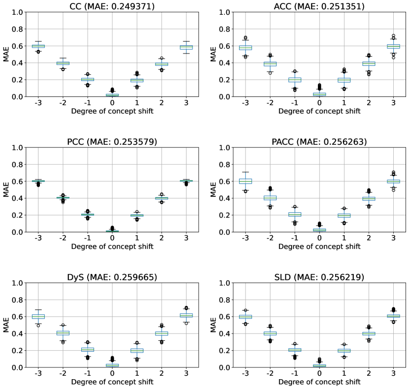
Figure 12: Results for concept shift. The error measure is MAE and the degree of concept shift is computed as $c_{tr}-c_{tst}$.

5.6.2 Results

The results for our simulation of concept shift are shown in Figure 12. The performance of all methods decreases as the degree of concept shift increases, i.e., when $c^{L}<c^{U}$ (resp., $c^{L}>c^{U}$) all methods tend to overestimate (resp., underestimate) the true prevalence. That no method could fare well under concept shift was expected, for the simple reason that none of these methods has been designed to confront arbitrary changes in the functional relationship between covariates and classes. These results deserve no further discussion, and are here reported only for the sake of completeness (we omit the corresponding table, though).

What instead deserves some discussion is the fact that concept shift might, under certain circumstances, lead to erroneous interpretations of the relative merits of quantification methods. This confusion might arise when the bias of a quantifier gets partially compensated by the variation in the prior resulting from the change in the concept. This situation is reproduced in Figure 13, where we impose $p_{L}=0.5$ and $p_{U}=0.75$. Take a look at the errors produced by both methods when $(c^{L}-c^{U})=0$, i.e., when $c^{L}=c^{U}$. Note that in this case, there is no concept shift, but there is prior probability shift. (Recall that we chose $p_{L}=0.5$ and $p_{U}=0.75$ for this experiment). We know that PCC tends to deliver biased estimators, while SLD instead does not. This is witnessed by the fact that PCC yields an error close to MAE=0.15 (it tends to underestimate the test prevalence), while SLD obtains a very low error instead; let us call this bias the “global” bias. As we separate the cut points, we introduce a form of bias (a “local” bias) that interacts with the global one. For instance, imagine we train our classifier with 1-star and 2-stars acting as negative labels and (3, 4, 5) acting as positive ones. Assume that in test we instead have (1, 2, 3) stars acting as the negative labels and only (4, 5) as the positives. In this case, the classifier will now tend to classify as positive the test examples with 3 stars. This local overestimation will partially compensate for the global underestimation. (An analogous reasoning applies in the other direction as well.) Note that such an improvement is accidental, and attributing any merit to the quantifier for this would be misleading.

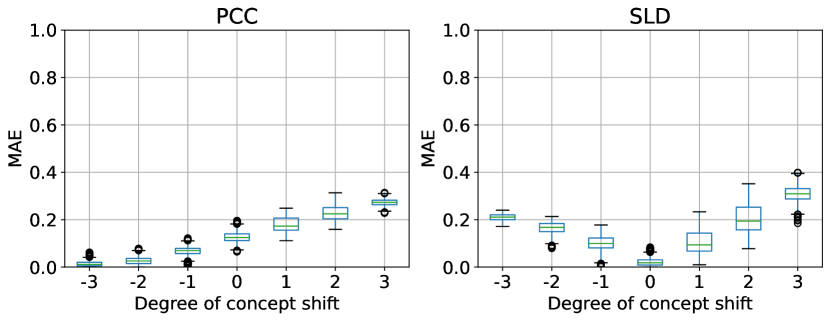
Figure 13: Results for concept shift with forced values for $p_{L}=0.5$ and $p_{U}=0.75$. The error measure is MAE and the degree of concept shift is computed as $(c_{tr}-c_{tst})$.

6 Conclusions

Since the goal of quantification is estimating class prevalence, most previous efforts in the field have focused on assessing the performance of quantification systems in situations characterised by a shift in class prevalence values, i.e., by prior probability shift; in the quantification literature other types of dataset shift have received less attention, if any. In this paper we have proposed new evaluation protocols for simulating different types of dataset shift in a controlled manner, and we have used them to test the robustness to these types of shift of several representative methods from the quantification literature. The experimental evaluation we have carried out has brought about some interesting findings.

The first such finding is that many quantification methods are robust to prior probability shift but not to other types of dataset shift. When the simplifying assumptions that characterise prior probability shift (e.g., that the class-conditional densities remain unaltered) are not satisfied, all the tested methods (including SLD, a top performer under prior probability shift) experience a marked degradation in performance.

A second observation is that, while previous theoretical studies indicate that PCC should be the best quantification method for dealing with covariate shift, our experiments reveal that its use should only be recommended when the class label proportions are expected not to change substantially (a setting that we refer to as pure covariate shift).

Such a setting, though, is fairly uninteresting in real-life applications, and our experiments show that other methods (particularly: SLD and PACC) are preferable to PCC when covariate shift is accompanied by a change in the priors. However, even SLD becomes unstable under certain conditions in which both covariates and labels change. We argue that such a setting, which we have called local covariate shift, shows up in many applications of interest (e.g., prevalence estimation of plankton subspecies in sea water samples (González et al., 2019), or seabed cover mapping (Beijbom et al., 2015), in which finer-grained unobserved classes are grouped into coarser-grained observed classes.

Finally, our results highlight the limitations that all quantification methods exhibit when coping with concept shift. This was to be expected since no method can adapt to arbitrary changes in the functional relationship between covariates and classes without the aid of external information. The same batch of experiments also shows that concept shift may induce a change in the priors that can partially compensate the bias of a quantifier; however, such an improvement is illusory and accidental, and it is difficult to envision clever ways for taking advantage of this phenomenon.

Possible directions for future work include extending the protocols we have devised to other specific types of shift that may be application-dependent (e.g., shifts due to transductive active learning (Kottke et al., 2022), to oversampling of positive training examples in imbalanced data scenarios (Moreo et al., 2016), to concept shifts in cross-lingual applications), and to types of quantification other than binary (e.g., multiclass, ordinal, multi-label). The goal of such research, as well of the research presented in this paper, is to allow a correct evaluation of the potential of different quantification methods when confronted with the different ways in which the unlabelled data we want to quantify on differs from the training data, and to stimulate research in new quantification methods capable of tackling the types of shift that current methods are insufficiently equipped for.

Appendix A The Equivalence of SMM and PACC

In this section we prove that the method Sample Mean Matching (SMM) proposed by Hassan et al. (2020) is equivalent to the method Probabilistic Adjusted Classify & Count (PACC) presented by Bella et al. (2010). This equivalence between the two methods was already hinted at in (Castaño et al., 2023) but no formal proof was provided.

SMM fits in the DyS framework of Maletzke et al. (2019), replacing histograms, binning the posterior probabilities issued by a soft classifier $s$, with the mean of these posteriors, and adopting $L_{1}$ as the dissimilarity function $DS$:

$$\hat{p}_{\sigma}^{\operatorname{SMM}}=\operatorname*{argmin}_{0\leq\alpha\leq 1}{|(\alpha\operatorname{\mathbb{E}}_{\mathbf{x}\in L^{\oplus}}\left[s(\mathbf{x})\right]+(1-\alpha)\operatorname{\mathbb{E}}_{\mathbf{x}\in L^{\ominus}}\left[s(\mathbf{x})\right])-\operatorname{\mathbb{E}}_{\mathbf{x}\in\sigma}\left[s(\mathbf{x})\right]|}$$ (10)

Solving for $\alpha$ when the $L_{1}$ distance is equal to 0 we obtain

$$\hat{p}_{\sigma}^{\operatorname{SMM}}=\frac{\operatorname{\mathbb{E}}_{\mathbf{x}\in\sigma}\left[s(\mathbf{x})\right]-\operatorname{\mathbb{E}}_{\mathbf{x}\in L^{\ominus}}\left[s(\mathbf{x})\right]}{\operatorname{\mathbb{E}}_{\mathbf{x}\in L^{\oplus}}\left[s(\mathbf{x})\right]-\operatorname{\mathbb{E}}_{\mathbf{x}\in L^{\ominus}}\left[s(\mathbf{x})\right]}.$$ (11)

On the other hand PACC solves the following equation to compute $\hat{p}^{\operatorname{PACC}}$:

$$\hat{p}_{\sigma}^{\operatorname{PACC}}=\frac{\hat{p}_{\sigma}^{\operatorname{PCC}}-\hat{\operatorname{fpr}}_{s}}{\hat{\operatorname{tpr}}_{s}-\hat{\operatorname{fpr}}_{s}}$$ (12)

Both Equations 11 and 12 are equal, as all their terms are equivalent:

$$\operatorname{\mathbb{E}}_{\mathbf{x}\in\sigma}\left[s(\mathbf{x})\right]= \ \frac{1}{|\sigma|}\sum_{x\in\sigma}{s(\mathbf{x})}\equiv\hat{p}_{\sigma}^{\operatorname{PCC}}$$ (13)

$$\operatorname{\mathbb{E}}_{\mathbf{x}\in L^{\ominus}}\left[s(\mathbf{x})\right]= \ \frac{1}{|L^{\ominus}|}\sum_{x\in L^{\ominus}}{s(\mathbf{x})}\equiv\hat{\operatorname{fpr}}_{s}$$ (14)

$$\operatorname{\mathbb{E}}_{\mathbf{x}\in L^{\oplus}}\left[s(\mathbf{x})\right]= \ \frac{1}{|L^{\oplus}|}\sum_{x\in L^{\oplus}}{s(\mathbf{x})}\equiv\hat{\operatorname{tpr}}_{s}$$ (15)

References

- Alaíz-Rodríguez et al. (2011) Alaíz-Rodríguez R, Guerrero-Curieses A, Cid-Sueiro J (2011) Class and subclass probability re-estimation to adapt a classifier in the presence of concept drift. Neurocomputing 74(16):2614–2623, DOI 10.1016/j.neucom.2011.03.019
- Alexandari et al. (2020) Alexandari A, Kundaje A, Shrikumar A (2020) Maximum likelihood with bias-corrected calibration is hard-to-beat at label shift adaptation. In: Proceedings of the 37th International Conference on Machine Learning (ICML 2020), Virtual Event, pp 222–232
- Azizzadenesheli et al. (2019) Azizzadenesheli K, Liu A, Yang F, Anandkumar A (2019) Regularized learning for domain adaptation under label shifts. In: Proceedings of the 7th International Conference on Learning Representations (ICLR 2019), New Orleans, US
- Barranquero et al. (2015) Barranquero J, Díez J, del Coz JJ (2015) Quantification-oriented learning based on reliable classifiers. Pattern Recognition 48(2):591–604, DOI 10.1016/j.patcog.2014.07.032
- Beijbom et al. (2015) Beijbom O, Hoffman J, Yao E, Darrell T, Rodriguez-Ramirez A, Gonzalez-Rivero M, Hoegh-Guldberg O (2015) Quantification in-the-wild: Data-sets and baselines, coRR abs/1510.04811 (2015). Presented at the NIPS 2015 Workshop on Transfer and Multi-Task Learning, Montreal, CA
- Bella et al. (2010) Bella A, Ferri C, Hernández-Orallo J, Ramírez-Quintana MJ (2010) Quantification via probability estimators. In: Proceedings of the 11th IEEE International Conference on Data Mining (ICDM 2010), Sydney, AU, pp 737–742, DOI 10.1109/icdm.2010.75
- Bickel et al. (2009) Bickel S, Brückner M, Scheffer T (2009) Discriminative learning under covariate shift. Journal of Machine Learning Research 10:2137–2155, DOI 10.5555/1577069.1755858
- Card and Smith (2018) Card D, Smith NA (2018) The importance of calibration for estimating proportions from annotations. In: Proceedings of the 2018 Conference of the North American Chapter of the Association for Computational Linguistics (HLT-NAACL 2018), New Orleans, US, pp 1636–1646, DOI 10.18653/v1/n18-1148
- Castaño et al. (2023) Castaño A, Alonso J, González P, del Coz JJ (2023) An equivalence analysis of binary quantification methods. In: Proceedings of the 37th AAAI Conference on Artificial Intelligence (AAAI-23), Washington, US, pp 6944–6952
- Chan and Ng (2006) Chan YS, Ng HT (2006) Estimating class priors in domain adaptation for word sense disambiguation. In: Proceedings of the 44th Annual Meeting of the Association for Computational Linguistics (ACL 2006), Sydney, AU, pp 89–96
- Chen et al. (2022) Chen L, Zaharia M, Zou J (2022) Estimating and explaining model performance when both covariates and labels shift. arXiv:2209.08436 [stat.ML]
- Dempster et al. (1977) Dempster AP, Laird NM, Rubin DB (1977) Maximum likelihood from incomplete data via the EM algorithm. Journal of the Royal Statistical Society, B 39(1):1–38
- du Plessis and Sugiyama (2012) du Plessis MC, Sugiyama M (2012) Semi-supervised learning of class balance under class-prior change by distribution matching. In: Proceedings of the 29th International Conference on Machine Learning (ICML 2012), Edinburgh, UK
- Esuli and Sebastiani (2010) Esuli A, Sebastiani F (2010) Machines that learn how to code open-ended survey data. International Journal of Market Research 52(6):775–800, DOI 10.2501/s147078531020165x
- Esuli and Sebastiani (2015) Esuli A, Sebastiani F (2015) Optimizing text quantifiers for multivariate loss functions. ACM Transactions on Knowledge Discovery and Data 9(4):Article 27, DOI 10.1145/2700406
- Esuli et al. (2018) Esuli A, Moreo A, Sebastiani F (2018) A recurrent neural network for sentiment quantification. In: Proceedings of the 27th ACM International Conference on Information and Knowledge Management (CIKM 2018), Torino, IT, pp 1775–1778, DOI 10.1145/3269206.3269287
- Esuli et al. (2022) Esuli A, Moreo A, Sebastiani F, Sperduti G (2022) A detailed overview of LeQua 2022: Learning to quantify. In: Working Notes of the 13th Conference and Labs of the Evaluation Forum (CLEF 2022), Bologna, IT
- Esuli et al. (2023) Esuli A, Fabris A, Moreo A, Sebastiani F (2023) Learning to quantify. Springer Nature, Cham, CH
- Fawcett and Flach (2005) Fawcett T, Flach P (2005) A response to Webb and Ting’s ‘On the application of ROC analysis to predict classification performance under varying class distributions’. Machine Learning 58(1):33–38, DOI 10.1007/s10994-005-5256-4
- Fernandes Vaz et al. (2019) Fernandes Vaz A, Izbicki R, Bassi Stern R (2019) Quantification under prior probability shift: The ratio estimator and its extensions. Journal of Machine Learning Research 20:79:1–79:33
- Flach (2017) Flach PA (2017) Classifier calibration. In: Sammut C, Webb GI (eds) Encyclopedia of Machine Learning, 2nd edn, Springer, Heidelberg, DE, pp 212–219
- Forman (2005) Forman G (2005) Counting positives accurately despite inaccurate classification. In: Proceedings of the 16th European Conference on Machine Learning (ECML 2005), Porto, PT, pp 564–575, DOI 10.1007/11564096“˙55
- Forman (2008) Forman G (2008) Quantifying counts and costs via classification. Data Mining and Knowledge Discovery 17(2):164–206, DOI 10.1007/s10618-008-0097-y
- González et al. (2017) González P, Castaño A, Chawla NV, del Coz JJ (2017) A review on quantification learning. ACM Computing Surveys 50(5):74:1–74:40, DOI 10.1145/3117807
- González et al. (2019) González P, Castaño A, Peacock EE, Díez J, Del Coz JJ, Sosik HM (2019) Automatic plankton quantification using deep features. Journal of Plankton Research 41(4):449–463
- González-Castro et al. (2013) González-Castro V, Alaiz-Rodríguez R, Alegre E (2013) Class distribution estimation based on the Hellinger distance. Information Sciences 218:146–164, DOI 10.1016/j.ins.2012.05.028
- Hassan et al. (2020) Hassan W, Maletzke AG, Batista GE (2020) Accurately quantifying a billion instances per second. In: Proceedings of the 7th IEEE International Conference on Data Science and Advanced Analytics (DSAA 2020), Sydney, AU, pp 1–10, DOI 10.1109/DSAA49011.2020.00012
- Hassan et al. (2021) Hassan W, Maletzke A, Batista G (2021) The risks of using classification datasets in quantification assessment. In: Proceedings of the 1st International Workshop on Learning to Quantify (LQ 2021), Gold Coast, AU
- Hofer and Krempl (2012) Hofer V, Krempl G (2012) Drift mining in data: A framework for addressing drift in classification. Computational Statistics & Data Analysis 57(1):377–391
- Hopkins and King (2010) Hopkins DJ, King G (2010) A method of automated nonparametric content analysis for social science. American Journal of Political Science 54(1):229–247, DOI 10.1111/j.1540-5907.2009.00428.x
- Iyer et al. (2014) Iyer A, Nath S, Sarawagi S (2014) Maximum mean discrepancy for class ratio estimation: Convergence bounds and kernel selection. In: Proceedings of the 31st International Conference on Machine Learning (ICML 2014), Beijing, CN, pp 530–538
- King and Lu (2008) King G, Lu Y (2008) Verbal autopsy methods with multiple causes of death. Statistical Science 23(1):78–91, DOI 10.1214/07-sts247
- Kottke et al. (2022) Kottke D, Sandrock C, Krempl G, Sick B (2022) A stopping criterion for transductive active learning. In: Proceedings of the 33rd European Conference on Machine Learning and Principles and Practice of Knowledge Discovery in Databases (ECML / PKDD 2022), Grenoble, FR, pp 468–484, DOI 10.1007/978-3-031-26412-2“˙29
- Kull and Flach (2014) Kull M, Flach P (2014) Patterns of dataset shift. In: First international workshop on learning over multiple contexts (LMCE) at ECML-PKDD, vol 5
- Lipton et al. (2018) Lipton ZC, Wang Y, Smola AJ (2018) Detecting and correcting for label shift with black box predictors. In: Proceedings of the 35th International Conference on Machine Learning (ICML 2018), Stockholm, SE, pp 3128–3136
- Maletzke et al. (2019) Maletzke A, Moreira dos Reis D, Cherman E, Batista G (2019) DyS: A framework for mixture models in quantification. In: Proceedings of the 33rd AAAI Conference on Artificial Intelligence (AAAI 2019), Honolulu, US, pp 4552–4560
- McAuley et al. (2015) McAuley JJ, Targett C, Shi Q, van den Hengel A (2015) Image-based recommendations on styles and substitutes. In: Proceedings of the 38th International ACM Conference on Research and Development in Information Retrieval (SIGIR 2015), Santiago, CL, pp 43–52, DOI 10.1145/2766462.2767755
- Milli et al. (2013) Milli L, Monreale A, Rossetti G, Giannotti F, Pedreschi D, Sebastiani F (2013) Quantification trees. In: Proceedings of the 13th IEEE International Conference on Data Mining (ICDM 2013), Dallas, US, pp 528–536, DOI 10.1109/icdm.2013.122
- Moreno-Torres et al. (2012) Moreno-Torres JG, Raeder T, Alaíz-Rodríguez R, Chawla NV, Herrera F (2012) A unifying view on dataset shift in classification. Pattern Recognition 45(1):521–530, DOI 10.1016/j.patcog.2011.06.019
- Moreo and Sebastiani (2021) Moreo A, Sebastiani F (2021) Re-assessing the “classify and count” quantification method. In: Proceedings of the 43rd European Conference on Information Retrieval (ECIR 2021), Lucca, IT, vol II, pp 75–91
- Moreo and Sebastiani (2022) Moreo A, Sebastiani F (2022) Tweet sentiment quantification: An experimental re-evaluation. PLOS ONE 17(9):1–23, DOI 10.1371/journal.pone.0263449
- Moreo et al. (2016) Moreo A, Esuli A, Sebastiani F (2016) Distributional random oversampling for imbalanced text classification. In: Proceedings of the 39th ACM Conference on Research and Development in Information Retrieval (SIGIR 2016), Pisa, IT, pp 805–808, DOI 10.1145/2911451.2914722
- Moreo et al. (2021) Moreo A, Esuli A, Sebastiani F (2021) QuaPy: A Python-based framework for quantification. In: Proceedings of the 30th ACM International Conference on Knowledge Management (CIKM 2021), Gold Coast, AU, pp 4534–4543, DOI 10.1145/3459637.3482015
- Nguyen et al. (2015) Nguyen TD, du Plessis MC, Sugiyama M (2015) Continuous target shift adaptation in supervised learning. In: Proceedings of the 7th Asian Conference on Machine Learning (ACML 2015), Hong Kong, CN, pp 285–300
- Pérez-Gállego et al. (2019) Pérez-Gállego P, Castaño A, Quevedo JR, del Coz JJ (2019) Dynamic ensemble selection for quantification tasks. Information Fusion 45:1–15, DOI 10.1016/j.inffus.2018.01.001
- Quiñonero-Candela et al. (2009) Quiñonero-Candela J, Sugiyama M, Schwaighofer A, Lawrence ND (eds) (2009) Dataset shift in machine learning. The MIT Press, Cambridge, US, DOI 10.7551/mitpress/9780262170055.001.0001
- Rabanser et al. (2019) Rabanser S, Günnemann S, Lipton ZC (2019) Failing loudly: An empirical study of methods for detecting dataset shift. In: Proceedings of the 32nd Conference on Neural Information Processing Systems (NeurIPS 2019), Vancouver, CA, pp 1394–1406
- Saerens et al. (2002) Saerens M, Latinne P, Decaestecker C (2002) Adjusting the outputs of a classifier to new a priori probabilities: A simple procedure. Neural Computation 14(1):21–41, DOI 10.1162/089976602753284446
- Schölkopf et al. (2012) Schölkopf B, Janzing D, Peters J, Sgouritsa E, Zhang K, Mooij JM (2012) On causal and anticausal learning. In: Proceedings of the 29th International Conference on Machine Learning (ICML 2012), Edinburgh, UK
- Schumacher et al. (2021) Schumacher T, Strohmaier M, Lemmerich F (2021) A comparative evaluation of quantification methods. arXiv:2103.03223v1 [cs.LG]
- Sebastiani (2020) Sebastiani F (2020) Evaluation measures for quantification: An axiomatic approach. Information Retrieval Journal 23(3):255–288, DOI 10.1007/s10791-019-09363-y
- Šipka et al. (2022) Šipka T, Šulc M, Matas J (2022) The hitchhiker’s guide to prior-shift adaptation. In: Proceedings of the IEEE Winter Conference on Applications of Computer Vision (WACV 2022), Waikoloa, US, pp 1516–1524
- Souza et al. (2020) Souza V, dos Reis DM, Maletzke AG, Batista GE (2020) Challenges in benchmarking stream learning algorithms with real-world data. Data Mining and Knowledge Discovery 34(6):1805–1858
- Storkey (2009) Storkey A (2009) When training and test sets are different: Characterizing learning transfer. In: Quiñonero-Candela J, Sugiyama M, Schwaighofer A, Lawrence ND (eds) Dataset shift in machine learning, The MIT Press, Cambridge, US, pp 3–28
- Tasche (2017) Tasche D (2017) Fisher consistency for prior probability shift. Journal of Machine Learning Research 18:95:1–95:32
- Tasche (2022) Tasche D (2022) Class prior estimation under covariate shift: No problem? arXiv:2206.02449 [stat.ML]
- Tasche (2023) Tasche D (2023) Invariance assumptions for class distribution estimation. In: Proceedings of the 3rd International Workshop on Learning to Quantify (LQ 2023), Torino, IT, pp 56–71
- Vucetic and Obradovic (2001) Vucetic S, Obradovic Z (2001) Classification on data with biased class distribution. In: Proceedings of the 12th European Conference on Machine Learning (ECML 2001), Freiburg, DE, pp 527–538
- Zhang et al. (2013) Zhang K, Schölkopf B, Muandet K, Wang Z (2013) Domain adaptation under target and conditional shift. In: Proceedings of the 30th International Conference on Machine Learning (ICML 2013), Atlanta, US, pp 819–827