Accelerating Pythonic coupled cluster implementations: a comparison between CPUs and GPUs

Abstract

We scrutinize how to accelerate the bottleneck operations of Pythonic coupled cluster implementations performed on a NVIDIA Tesla V100S PCIe 32GB (rev 1a) Graphics Processing Unit (GPU). The NVIDIA Compute Unified Device Architecture (CUDA) API is interacted with via CuPy, an open-source library for Python, designed as a NumPy drop-in replacement for GPUs. The implementation uses the Cholesky linear algebra domain and is done in PyBEST, the Pythonic Black-box Electronic Structure Tool—a fully-fledged modern electronic structure software package. Due to the limitations of Video Memory (VRAM), the GPU calculations must be performed batch-wise. Timing results of some contractions containing large tensors are presented. The CuPy implementation leads to factor 10 speed-up compared to calculations on 36 CPUs. Furthermore, we benchmark several Pythonic routines for time and memory requirements to identify the optimal choice of the tensor contraction operations available. Finally, we compare an example CCSD and pCCD-LCCSD calculation performed solely on CPUs to their CPU–GPU hybrid implementation. Our results indicate a significant speed-up (up to a factor of 16 regarding the bottleneck operations) when offloading specific contractions to the GPU using CuPy.

1 Introduction

A critical job of a Graphics card is to compute projections of 3-dimensional objects to a 2D surface using linear algebra. These calculations can be performed in parallel very effectively, meaning that multiple small mathematical operations like multiplication and addition can be performed simultaneously. For this reason, Graphics Processing Unit (GPU) development mainly focuses on massively increasing the number of computing cores. While a Central Processing Unit (CPU) may have up to 128 cores on the high end, GPUs already have up to 16,000 cores (like NVIDIA RTX 4090).

In scientific computing, the distribution of calculations among multiple CPU cores and multiple nodes is a standard practice. ^{1, 2, 3, 4, 5} Due to its inherently parallel structure, linear algebra operations can be calculated in parallel and, therefore, efficiently offloaded to the GPU. ^{6, 7, 8, 9, 10} The first to report independently that the internal hugely parallel structure of GPUs can be misused, not to compute graphics, but to be utilized in quantum chemistry were Yasuda ¹¹ and Ufimtsev and Martinez,¹² respectively. Today, the potential of GPUs for non-graphics-related computations is widely understood and often used to accelerate quantum chemistry methods like density functional approximations ¹³, Hartree–Fock theory ^{14, 15}, Møller–Plesset perturbation theory ^{16, 17, 18}, coupled cluster theory ^{8, 19, 20, 3, 21}, and the evaluation of effective core potentials ²² to name a few. The NVIDIA CUDA API offers a C++ interface to utilize GPU computing power. ^{23, 24} A relatively quick way to interact with this API is, for example, CuPy ²⁵, a Python library which internally uses CUDA routines. CuPy brings a lot of attention from Python-based software developers as its interface is highly compatible with NumPy ²⁶ and allows even for a drop-in replacement in some particular cases. Although sacrificing some fine control when exploiting libraries like CuPy, third-party libraries are quickly accessible without the necessity of in-detail back-end control and, therefore, a very convenient and efficient way to probe graphics processor utilization in the first place.

In this work, we will present benchmark results comparing the timings of the bottleneck tensor contractions present in coupled-cluster calculations restricted to at most double excitations, where Cholesky vectors approximate the electron repulsion integrals. ²⁷ Specifically, we propose several flavors of performing these bottleneck contractions on a CPU using Pythonic libraries and benchmark their resource requirements. These contractions are calculated with, for instance, NumPy’s ²⁶ tensordot and einsum routines or opt_einsum ²⁸ on CPUs. Finally, we elaborate on exporting these operations on a GPU exploiting CuPy’s tensordot routine. ²⁵

This work is organized as follows. In section 2, we briefly discuss the main bottleneck operations in coupled-cluster calculations. Section 3 scrutinizes several Python-based strategies to compute the coupled-cluster vector function. In section 4, we examine the PyBEST tensor contraction engine. A GPU implementation exploiting the CuPy library is summarized in section 5. Numerical results and assessment of the GPU to CPU performance are presented in section 6. Finally, we conclude in section 7.

2 The CC ansatz

Our starting point is the coupled cluster (CC) ansatz ^{29, 30, 31, 32, 33, 34},

$$\ket{\Psi}=e^{\hat{T}}\ket{\Phi_{0}}$$ (1)

where $\hat{T}$ is the cluster operator and $\ket{\Phi_{0}}$ some reference wave function like the Hartree–Fock determinant. In this work, we will consider, at most, double excitations in the cluster operator, that is, $\hat{T}=\hat{T}_{2}$. We do not consider single excitations explicitly as the bottleneck operations are due to the $\hat{T}_{2}$ excitation operator. Furthermore, we will work in the spin-free representation, with spin-free amplitudes, and the CC equations are spin summed. In this picture, the double excitation operator takes on the form

$$\hat{T}_{2}=\frac{1}{2}\sum_{ij}^{\rm occ}\sum_{ab}^{\rm virt}t_{ij}^{ab}\hat{E}_{ai}\hat{E}_{bj}$$ (2)

with the CCD amplitude $t_{ij}^{ab}$ and $\hat{E}_{ai}$ being the singlet excitation operator,

$$\hat{E}_{ai}=\hat{a}^{\dagger}\hat{i}+\hat{\bar{a}}^{\dagger}\hat{\bar{i}},$$ (3)

where $p^{\dagger}$ ($\bar{p}^{\dagger}$) indicates electron creation operators for $\alpha$ ($\beta$) electrons, while $p$ ($\bar{p}$) are the corresponding annihilation operators. The above sum runs over all occupied (occ) and virtual (virt) orbitals for the chosen reference determinant $\ket{\Phi_{0}}$.

The scaling-determining step in the CCD amplitude equations is associated with the following term

$$0=\ldots+\sum_{cd}\bra{ab}\ket{cd}t_{ij}^{cd}+\ldots$$ (4)

Summation over the indices $i,j,a,b$ is implied, which results in the formal scaling of the CCD equations of $\mathcal{O}(o^{2}v^{4})$. In the above equation, $\bra{ab}\ket{cd}$ are the electron-repulsion integrals in Physicist’s notation. To reduce the storage of the full electron-repulsion integrals, they can be approximated by Cholesky decomposition, ^{35, 27}

$$\bra{ab}\ket{cd}\approx\sum_{x}L_{ac}^{x}L_{bd}^{x},$$ (5)

where $x$ indicates the summation over the elements of the Cholesky vectors. Since we work with real orbitals with 8-fold permutational symmetry of the electron-repulsion integrals (ERI), both Cholesky vectors $L_{ac}^{x}$ and $L_{bd}^{x}$ are identical. Then, the CC excitation amplitudes are optimized iteratively by rewriting the rate-determining step of the vector function $\tilde{t}_{ij}^{ab}$ of iteration $n$ of the optimization procedure,

$$\tilde{t}_{ij}^{ab}=\ldots+\sum_{xcd}L_{ac}^{x}L_{bd}^{x}t_{ij}^{cd}+\ldots,$$ (6)

including a third summation index running over the Cholesky vectors (ignoring the summation over the fixed indices $i,j,a,b$). Thus, formally, the complexity increases to $\mathcal{O}(xo^{2}v^{4})$. Note that the dimension of $x$ depends on the chosen threshold of the Cholesky decomposition. For decent to tight thresholds (around $10^{-6}$), we have $x\approx 5(o+v)$.

3 Pythonic implementations of the CC vector function

To solve for the CC amplitudes iteratively, we must evaluate the vector function of eq. (6) in each iteration, including all its terms. Thus, we will focus on the bottleneck operations of the corresponding CCD vector function. Within a Pythonic implementation, we can utilize various Python libraries to perform summations efficiently without resorting to a nested for-loop implementation. ^{36, 37, 38, 39, 40, 41} Based on the chosen routines, these summations (in the following called contractions) can be performed in one shot or sequentially, creating several intermediates to boost efficiency and reduce resource requirements or even enabling out-of-the-box parallelization. In the following, we will scrutinize different variants to evaluate eq. (6) as pythonically as possible, focusing solely on Python features and libraries. Specifically, we focus on the NumPy routines einsum and tensordot, the opt_einsum package, and a GPU implementation exploiting CuPy’s tensordot feature.

3.1 einsum and opt_einsum

The possibly easiest and most straightforward way of avoiding nested for-loop implementations when dealing with tensor contractions is to refer to NumPy’s einsum routine, which evaluates the Einstein summation convention on a sequence of operands. Using numpy.einsum, many—albeit not all—linear algebraic operations on multi-dimensional arrays can be represented in a simple and intuitive language. With increasing version number, additional features and improvements have been incorporated into the numpy.einsum function. One crucial parameter is the optimize argument, which allows control over intermediate optimization. If set to "optimal", an optimal path of the contraction in question will be performed. Another possibility is to exploit the numpy.einsum_path function to steer the order of the individual contractions in the most optimal way.

An effort to improve the performance of the original numpy.einsum routine lead to the development of the opt_einsum package. ²⁸ It offers several features to optimize numpy.einsum significantly, reducing the overall execution time of einsum-like expressions. For instance, it automatically optimizes the order of the underlying contraction and exploits specialized routines or BLAS ⁴². opt_einsum can also handle various arrays, like NumPy, Dask, PyTorch, Tensorflow, or CuPy, to name a few. Furthermore, the optimization of numpy.einsum has been passed upstream to the original numpy.einsum project. Some of opt_einsum’s features can hence be utilized by numpy.einsum modifying the optimization option. Since opt_einsum features more up-to-date algorithms for complex contractions, we will focus on the opt_einsum.contract function to evaluate the Einstein summation convention on a sequence of operands, typically containing three multi-dimensional input arrays.

opt_einsum.contract represents a replacement for numpy.einsum where the order of the contraction is optimized to reduce the overall scaling (and hence increase the computational speed-up) at the cost of several intermediate arrays. To steer the memory limit and prevent the generation of too large intermediates, opt_einsum.contract offers the memory_limit parameter to provide an upper bound of the largest intermediate array built during the tensor contraction.

Thus, the bottleneck contraction in eq. (6) can be straightforwardly evaluated using, for instance, opt_einsum.contract as follows

⬇

t_new[:] += opt_einsum.contract("xac,xbd,icjd->iajb", L_0, L_1, t_old)

In the above code snippet, t_new indicates the vector function of iteration $n$, t_old the current approximate solution of the CCD amplitudes, L_0 (L_1) is the Cholesky vector of eq. (5). Note that $\tilde{t}_{ij}^{ab}$ are stored as a 4-dimensional NumPy array t_new[i,a,j,b].

3.2 tensordot

An alternative routine to perform a tensor contraction is the tensordot function offered in NumPy⁴³ and CuPy²⁵. It efficiently computes the summation of one (or more) given index (indices). It allows for saving memory by de-allocating intermediate arrays and explicitly defining the path of the complete tensor contraction. Furthermore, tensordot makes use of the BLAS⁴² API and features a multithreaded implementation when linked against the proper libraries like OpenBLAS, ⁴⁴ MKL, ⁴⁵ or ATLAS. ⁴⁶ A contraction along one axis of two arrays A and B,

$$C_{ij}=\sum_{n}A_{ni}B_{nj},$$

translates into

⬇

C = tensordot(A, B, axes=([0, 0]))

Similarly, tensordot can contract (that is, sum over) two or more axes in one function call, where

$$C_{ij\ldots kl}=\sum_{nm\ldots}A_{nimj\ldots}B_{nklm\ldots},$$

translates into

⬇

C = tensordot(A, B, axes=([0,1], [0,2]))

Note, however, that tensordot allows for contracting only two operands at a time. Thus, to evaluate the term in eq. (6), a sequence of tensordot calls must be performed where suitable intermediates are created. One possibility is to contract the Cholesky vectors to create an intermediate of dimension $v^{4}$, which is then passed to a second tensordot call generating the desired output,

⬇

# first intermediate generates the dense ERI[a,c,b,d]

eri_acbd = tensordot(L_0, L_1, axes=([0, 0]))

# second contraction results in t_new[i,j,a,b]

t_new[:] += tensordot(t_old, eri_acbd, axes=([1,3], [1,3])).transpose((0,2,1,3))

Note that tensordot does not reorder the axis. In that case, we need to transpose the intermediate result to match the shape of the output array (the vector function). However, generating a $v^{4}$ intermediate of the ERI might be prohibitive regarding memory requirements for larger systems. Other possibilities lead to even larger intermediates. For instance, contracting L_0 with t_old yields a multi-dimensional array of size $xo^{2}v^{3}$, which is smaller than the eri_acbd intermediate if $xo^{2}\ll v$, where $x$ is a pre-factor depending on the threshold of the Cholesky-decomposed ERI. This pre-factor is typically challenging to determine a priori. Nonetheless, for computationally feasible problems, the condition $ao^{2}\ll v$ is rarely satisfied, making the first contraction path computationally more efficient in terms of memory.

A less elegant, albeit computationally cheaper way to use all the benefits of the tensordot function is to introduce one for-loop to iterate over one axis. If we choose to loop over the second axis of L_0, we generate intermediates of at most $v^{3}$,

⬇

for a in range(L_0.shape[1]):

# first contract two Cholesky vectors

eri_bdc = numpy.tensordot(L_1, L_0[:, a, :], axes=([0, 0]))

# contract t_old[i,c,j,d] with eri_bdc (sum over c and d)

t_new[:, a, :, :] += tensordot(t_old, eri_bdc, axes=([1, 3], [2, 1]))

The following will refer to the contraction path above as our numpy.tensordot routine. Note, however, that this is not purely a numpy.tensordot computation, but an iterative call of the numpy.tensordot method to calculate eq. (6) to prevent the creation of $v^{4}$ intermediate tensors.

4 A modular implementation of tensor contractions

We have implemented and benchmarked the performance of the above-mentioned tensor contraction routines in PyBEST. ³⁷ Specifically, PyBEST is designed as a modular toolbox where the wave-function-specific implementations are decoupled from the linear algebra operations. In an actual calculation, the logic in choosing the optimal tensor-contraction scheme is as follows

⬇

try:

cupy-accelerated contraction

except NotImplementedError:

try:

numpy.tensordot contraction

except ArgumentError:

opt_einsum if not available then numpy.einsum(…, optimize="optimal")

The first try statement enforces that selected tensor contractions are performed on the GPU if available. If bottleneck-specific contractions are not supported, or a CUDA-ready GPU is unavailable, a numpy.tensordot call is performed. Since numpy.tensordot supports only specific contractions featuring non-repeating indices (that is, repeated indices have to be summed over in numpy.tensordot), an opt_einsum call is performed or, if opt_einsum is not available, an optimized numpy.einsum function call is made instead. The corresponding tensor contraction operation is written using the Einstein-summation convention of the numpy.einsum module, that is, all mathematical operations use an input and output string, where repeated indices are summed over. That allows for one unique notation of mathematical operations independent of the underlying representation of the tensors, especially the ERI. As an example, the bottleneck contraction in eq. (6) translates to the string "abcd,ecfd->eafb", where the first part (abcd) corresponds to the ERI, the second part (ecfd) to the doubles amplitudes, while the output string (eafb) indicates the order of the output indices of the vector function. Internally, this string is further decoded according to the notation used in the employed LinalgFactory instance, a dense or Cholesky-decomposed representation. If a dense representation of tensors is chosen, the string remains as is. For Cholesky-decomposed ERI, the input argument associated with the Cholesky instance (here "abcd") is translated to the internal Cholesky representation, that is, "xac,xbd".

Since numpy.tensordot only supports a summation over two multi-dimensional arrays at a time, we need to divide a tensor contraction containing more than two operands into appropriate intermediates. Such a partitioning can be fully automatized, exploiting the numpy.einsum_path function. It proposes a contraction order of lowest possible cost for an einsum expression, taking into account the creation of intermediate arrays. The resulting tensordot_helper function has the following logic

⬇

def tensordot_helper(subscripts, *operands):

# split subscripts in input and output strings

inscripts, outscript = split subscripts wrt "->"

# sanity check

if contraction cannot be performed:

raise ArgumentError(error message)

# get the optimial path

path, _ = numpy.einsum_path(subscripts, *operands)

# sometimes einsum_path does not return a list of two-element tuples

if no optimized path has been found:

path = provide some path

# loop over all steps in the path

for step in path[1:]:

# take 1st and 2nd operands and corresponding subscripts

op0, op1 = take the proper arrays from the operands list

# Find summation axes

axis0 = list containing axis indices to sum over for op0

axis1 = list containing axis indices to sum over for op1

axis = (axis0, axis1)

# find default outscript

outscript_ = store shape of intermediate

# do contraction using numpy.tensordot

outmat = numpy.tensordot(op0, op1, axes=axis)

# update the list of operands and subscripts used in the next interation

operands.append(outmat)

scripts.append(outscript_)

# do transposition if required.

if outscript does not have the proper shape:

trans = tuple how to transpose the output array

outmat = outmat.transpose(trans)

# return result of the tensor contraction

return outmat

The subscripts argument is a string specifying the contraction using the numpy.einsum notation, while all multi-dimensional input arrays are stored in the operands argument. We assume that the ERI corresponds to the leading subscripts. If a tensor contraction cannot be performed, we transition to opt_einsum or numpy.einsum(..., optimize="optimal") and an ArgumentError is raised. In case of too large intermediates, the tensordot_helper function is replaced by a function call containing selected hand-optimized tensor contraction operations. The implemented flow of contraction operations (CuPy–numpy.tensordot–opt_einsum/ numpy.einsum) allows for an optimal usage of computational resources, hardware, and multithreaded implementations. The reasons for the proposed operational flow are scrutinized in section 6. When the performance of the used libraries is improved in future releases, the order of the contraction flavors can be adjusted to maximize efficiency without significantly interfering with the underlying source code in each wave function module.

In the following, all benchmark calculations adhere to the contraction flow mentioned above if not stated otherwise. That is, the majority of tensor contractions are performed using the numpy.tensordot routine, while the bottleneck contractions are outsourced to the GPU.

5 CuPy and batch-wise computations

While, of course, the most performance one could achieve by designing a method specifically for the hardware to be calculated, we focus on accelerating the mathematical bottleneck operations by exporting the contractions in question to the GPU.

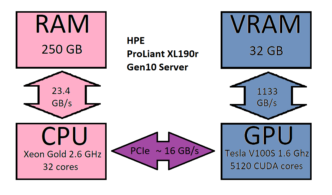
Figure 1: Schematic picture of RAM VRAM GPU and CPU and the data transfer rate between the components.

As proof of the concept, we exploit CuPy²⁵ for GPU-accelerated computing. Specifically, it is written as a drop-in replacement for NumPy⁴³. For medium- or large-sized molecules, we have to consider the size of the multi-dimensional arrays present in eq. (6) and, therefore, the amount of data that needs to be processed and transferred to the Video RAM (VRAM). The principle of memory and processor communication is shown in Fig. 1. Due to their size, the underlying multi-dimensional arrays might be too big to be transferred, processed on the GPU, and transferred back. Thus, a generic implementation, where a NumPy implementation is recycled as a CuPy implementation by replacing, for instance, numpy.einsum with cupy.einsum and taking into account host to device and device to host operations is impracticable or even impossible.

To calculate contractions on the GPU for realistic molecules and large basis sets, it is necessary to do the computations in batches. In our batch-wise computing approach, the arrays on which the operations will be performed must be copied to the VRAM in chunks. To maximize performance and utilize the massive number of CUDA cores, the size of the chunks has to be chosen as big as possible so that as few as possible cycles are needed. To achieve reasonably-sized chunks of data to be processed in batches, we multiply the number of elements with their corresponding element size (in bytes) and sum up the required storage space for each multi-dimensional array involved. If too large, the arrays are split, and the necessary memory is checked again. This process is repeated till the split arrays fit into the video memory. An example that shows the splitting, allocations, and de-allocations is shown in the following code example for the contraction xac,xbd,ecfd->eafb:

⬇

t_new = numpy.zeros((t_old.shape[0], L_0.shape[1], t_old.shape[2], L_1.shape[1]))

start_e = 0

end_e = 0

# parts_d is the number of parts in which the dense array will be split

for e in range(0, parts_d):

end_e += dense_e_chunk_lengths[e]

start_a = 0

end_a = 0

# parts_c is the number of parts in which the Cholesky array will be split

for a in range(0, parts_c):

end_a += chol_chunk_lengths_0[a]

start_b = 0

end_b = 0

# parts_c is the number of parts in which the Cholesky array will be split

for b in range(0, parts_c):

end_b += chol_chunk_lengths_1[b]

# Batches of Cholesky arrays are copied to GPU Memory (VRAM)

chol_0 = cupy.array(numpy.array_split(L_0, parts_c, axis=1)[a])

chol_1 = cupy.array(numpy.array_split(L_1, parts_c, axis=1)[b])

# calculating batch of xac,xbd->acbd on GPU

result_temp = cupy.tensordot(chol_0, chol_1, axes=(0, 0))

# deallocation

del chol_0, chol_1

cupy.get_default_memory_pool().free_all_blocks()

# Batches of the vector function array is copied to VRAM

operand = cupy.array(numpy.array_split(t_old, parts_d, axis=0)[e])

# calculating batch of acbd,ecfd->abef on GPU

result_temp_2 = cupy.tensordot(

result_temp, operand,axes=([1, 3], [1, 3])

)

# deallocation

del operand, result_temp

cupy.get_default_memory_pool().free_all_blocks()

# calculating batch of the transposition abef->eafb on GPU

result_part = cupy.transpose(result_temp_2, axes=(2, 0, 3, 1))

# deallocation

del result_temp_2

cupy.get_default_memory_pool().free_all_blocks()

# result arrays are copied back to the memory (RAM)

t_new[

start_e:end_e, start_a:end_a, :, start_b:end_b

] = result_part.get()

# deallocation

del result_part

cupy.get_default_memory_pool().free_all_blocks()

start_b = end_b

start_a = end_a

start_e = end_e

6 Numerical results

6.1 Software specifications and computational details

All calculations were performed on the CentOS 7 operating system using, if not mentioned otherwise, the CUDA compilation tools v12.1.105, intelpython v3.9 (referred to as Python in the following), Intel OneAPI v2023.1, and CuPy v12.0.0. Furthermore we employed NumPy v1.23.5, opt_einsum v3.3.0, and PyBEST v1.4.0dev0. The hardware on which the computations were performed is gathered in section S1 of the Supporting Information. Note that for the benchmark data shown in Fig. 2, we used Intel Python 3.7, Intel OneAPI v2021.3, PyBEST v1.3.0, and NumPy v1.21.2.

The molecular structure of the L0 dye was optimized in the ORCA 5.0.3 software package ^{47, 48, 49, 50} using the B3LYP ^{51, 52} exchange–correlation functional and the cc-pVTZ basis set. ⁵³ The resulting structural parameters are provided in section S2 of the Supplementary Information. That molecular structure is subsequently used in the orbital-optimized pair coupled cluster doubles (pCCD ^{54, 55, 56, 57, 58, 59}) augmented with the linearized coupled cluster singles and doubles (pCCD-LCCSD) correction ⁶⁰, and the conventional coupled-cluster singles and doubles (CCSD) approach, as implemented in the PyBEST software package. ³⁷ In all PyBEST calculations for the L0 dye, we utilized the Cholesky linear algebra factory with a threshold of $10^{-5}$ for the ERI. In all benchmark calculations concerning timings and memory requirements, the Cholesky vectors are random arrays, where we assume a size of $5K^{3}$ with $K$ corresponding to the number of basis functions. This roughly corresponds to a Cholesky cutoff threshold of $10^{-5}$ in actual molecular calculations.

6.2 Comparison between CPU and GPU-accelerated implementations

To be able to make assumptions about the benefit of offloading computations to the GPU, it is reasonable to study how effectively different functions described in section 3 perform compared to each other. In the following, the computation times of numpy.tensordot, opt_einsum, and their CPU multicore processing behavior are investigated and compared with CuPy’s tensordot. As mentioned above, a very handy way for implementing tensor contractions is numpy.einsum or opt_einsum, which feature a similar syntax. We should note that although numpy.einsum and opt_einsum have similar performance if two operands are contracted with each other, this is not the case anymore if the list of operands contains several multi-dimensional arrays. In the latter case, opt_einsum may be superior to numpy in terms of computing time by several orders of magnitude, primarily due to the parallelization of the underlying lower-level opt_einsum routines. Thus, we only show benchmark results for opt_einsum in this work. Furthermore, we investigate three tensor contractions, namely "abcd,ecfd->eafb", "abcd,edfc->eafb", and "abcd,ecfd->efab". The first contraction ("abcd,ecfd->eafb") corresponds to the bottleneck term of eq. (6), while the second one is the associated exchange term, which reads

$$\sum_{xcd}L_{ad}^{x}L_{bc}^{x}t_{ij}^{cd}.$$ (7)

Although the exchange part of the formal bottleneck contraction is not present when working in a spin-free representation, we benchmark this contraction for reasons of completeness, in case a spin-dependent implementation is sought. The third contraction "abcd,ecfd->efab" recipe is used in two additional terms of the CCSD vector function. These are one term involving an intermediate $\tilde{t}_{ijkl}$,

$$\tilde{t}_{ijkl}=\sum_{xcd}L_{kc}^{x}L_{ld}^{x}t_{ij}^{cd},$$ (8)

which is an operation of $\mathcal{O}(xo^{4}v^{2})$ complexity, and another one comprising the ERI of $\mathcal{O}(ov^{3})$,

$$\tilde{t}_{ijbk}=\sum_{xcd}L_{bd}^{x}L_{kc}^{x}t_{ij}^{cd},$$ (9)

with computational complexity of $\mathcal{O}(xo^{3}v^{3})$. Note that exporting eq. (8) to the GPU is merely a byproduct of eq. (9) as both contraction can be written using the same subscript.

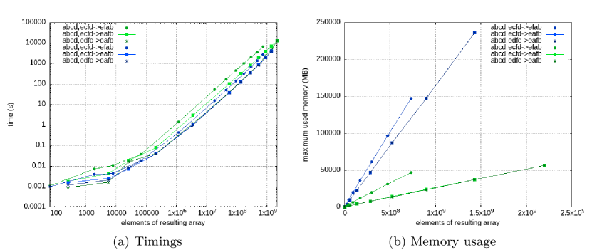
Figure 2: Timings (a) and memory usage (b) of numpy.tensordot and opt_einsum with respect to the size (number of elements) of the largest input array. In both plots, the greenish colors show tensordot and blueish colors show opt_einsum computations using 1 CPU core.

Compared to (our version of) numpy.tensordot, the internal optimization leads to a speed-up of factor 2 as indicated by Fig. 2(a). The reason we chose numpy.tensordot as the workhorse of all tensor contractions instead of opt_einsum (or numpy.einsum), is the severe disadvantage of opt_einsum regarding memory efficiency. This drawback becomes evident in the peak memory usage displayed in Fig. 2(b). The internal optimization and the creation of intermediate arrays (for speed-up) lead to a factor 3 faster-growing memory consumption. That disqualifies opt_einsum as a generic option primarily because we do not want to and often cannot constrain the code to smaller problem sizes. Therefore, we employ numpy.tensordot as the default contraction flavor if Nvidia CUDA is not available. We should note that opt_einsum features other arguments that limit the memory peak to a specific size. However, this feature comes at the cost of computing time. Specifically, a user-defined limit of the memory peak significantly deteriorates the speed of the numerical operations, which renders opt_einsum impractical for large-scale tensor contractions.

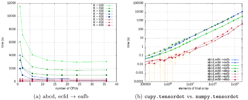
Figure 3: Computing times for CPU and GPU-accelerated implementations. (a) Timings for the bottleneck contraction abcd,ecfd->eafb. The greenish colors show numpy.tensordot, the blueish colors correspond to opt_einsum, while reddish colors indicate cupy.tensordot results. $K$ is the total number of basis functions. (b) Comparison of GPU and CPU computing times for different basis set sizes $K$. The numpy.tensordot results for calculations with 1 CPU thread are shown in blueish colors and for 36 CPU threads in greenish colors. The reddish colors show the cupy.tensordot results. The error bars in orange are determined for an average of 10 runs and show the standard deviation. For the number of elements of the final array, see the description in the main text.

Fig. 3(a) summarizes timings for computations of the contraction "abcd,ecfd->eafb" (or "xac,xbd,ecfd->eafb" if the Cholesky vectors are explicitly mentioned) plotted over the number of CPU cores for various tensor contraction flavors and problem sizes $N$. The greenish colors show numpy.tensordot, the blueish colors opt_einsum, while reddish colors indicate cupy.tensordot timing results for different numbers of CPU cores. Specifically for Fig. 3(a), the problem size is given by $N=o^{2}v^{2}$ because we investigate the following problem setup with dimensions $(xv^{2},xv^{2},o^{2}v^{2}\rightarrow o^{2}v^{2})$, where $v$ and $o$ are the number of virtual and occupied orbitals respectively. Their sizes have been set according to the relation $v=\mathrm{int}(\frac{3}{4}K)$ and $o=K-v$, where $K$ is the total number of basis functions. We should mention that the data for $K=500$ using opt_einsum could not be obtained due to technical problems as the memory consumption/memory peak exceeds the available physical memory of the computing node. Overall, the opt_einsum calculations are a factor $3$ faster than the corresponding numpy.tensordot variants but limited by their memory peak. Note, however, that the for-loop-based numpy.tensordot variant is roughly a factor of 2 slower compared to the contraction scheme where the $v^{4}$ intermediate is formed. Thus, opt_einsum and numpy.tensordot are comparable in performance, with the former being modestly faster.

Fig. 3(a) further highlights that the benefit of performing a computation on a larger number of cores shrinks very rapidly. The timings reach a plateau at about 8 to 10 cores. Judging by the numbers, the contraction functions do not really benefit from the usage of more than 10 cores, with 4 cores being the most reasonable amount, assuming the computing time is limited. The bigger the basis set or problem size the more benefit one gets from utilizing a higher number of cores. The cupy.tensordot timings are also shown in Fig. 3(a) for a direct comparison. We should note that they are independent of the number of CPU cores (as the mathematical operations are performed on the GPU) and faster than both the NumPy and opt_einsum alternatives.

	$N$
$K$	300	400	500
abcd,ecfd->eafb	284 765 625	900 000 000	2 197 265 625	$o^{2}v^{2}$
abcd,edfc->eafb	284 765 625	900 000 000	2 197 265 625	$o^{2}v^{2}$
abcd,ecfd->efab	94 921 875	300 000 000	732 421 875	$o^{3}v$

Table 1: Problem sizes $N$ determined for different basis set sizes $K$ for the selected contractions benchmarked in this work. The last column indicates the size of the output array.

Fig. 3(b) compares the required computing time of CPU and GPU-accelerated contractions. The results corresponding to GPU and CPU timings are taken as an average of over 10 runs. Furthermore, the CPU data was obtained from computations exploiting 1 and 36 CPU cores, respectively. Fig. 3(b) contains 3 different datasets, namely, one for each investigated contraction "abcd,ecfd->eafb", "abcd,edfc->eafb", and "abcd,ecfd->efab". Note that the notation is internally translated to the Cholesky vectors by replacing the "abcd" part of the string by "xac,xbd". Thus, we always have three input operands in each tensor contraction operation. We should stress that the timings corresponding to all three contraction subscripts are very close to each other making them almost indistinguishable from each other on the plot. For reasons of comparability, the x axis shows the problem size, which is given by the size of the resulting (output) tensor. Table 1 summarizes the different problem sizes with respect to the contraction subscript, namely, $N=o^{2}v^{2}$ for "abcd,ecfd->eafb" and "abcd,edfc->eafb" and $N=o^{3}v$ for the contraction "abcd,ecfd->efab", respectively. The standard deviation for the timings of larger problem sizes is about $1\%$ of the average value, while it increases to approximately $10\%$ for smaller problem sizes. The elements of the arrays used to perform the benchmark calculations were randomly generated. We attribute the larger standard deviation for smaller problem sizes to the higher impact a randomly generated array (e.g., very small numbers) can have, when among fewer elements in an operation.

All in all, we observe an order of magnitude reduction of computing time for the CuPy implementation computed on the NVIDIA Tesla V100S PCIe 32GB (rev 1a) compared to our NumPy implementation computed on 36 CPU cores for 3 different tensor contractions encountered in the CCSD working equations.

6.3 A case study — a sensitizer molecule

To check the overall speed-up in actual chemical problems, we will perform example calculations with and without GPU acceleration. Specifically, we will scrutinize the impact on the overall computing time when offloading just a given set of contractions to the GPU. 2-Cyano-3-(4-N,N-diphenylaminophenyl)-trans-acrylic acid, commonly referred to as L0 dye,⁶¹ has been chosen as the candidate for this performance test. This organic dye was designed to be a potential sensitizer in dye-sensitized solar cells, making it a viable alternative to ruthenium-type dyes. The size of the L0 dye allows us to benchmark the Python-based hybrid CPU–GPU implementation for a chosen parameter set.

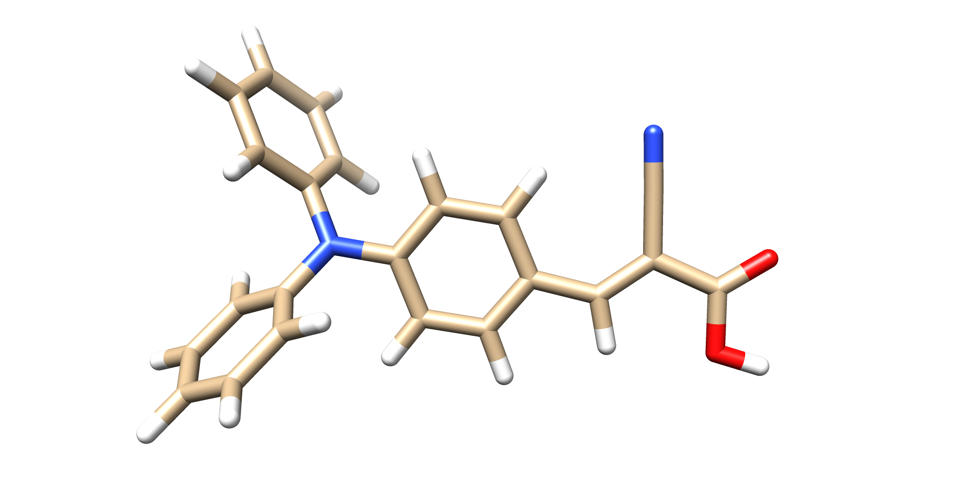
Figure 4: Molecular structure of the L0 dye relaxed at the B3LYP/cc-pVTZ level of theory.

		CCSD		pCCD-LCCSD
		NumPy	CuPy	NumPy	CuPy
Timings	Average iteration step (CPU+GPU)	2754.21	918.25	2692.91	813.80
	Average iteration step (CPU)	2754.21	795.28	2692.91	680.00
	Average iteration step (GPU)	–	122.98	–	133.80
	Vector function step (CPU+GPU)	2600.68	766.98	2541.80	662.38
	Vector function step (CPU)	2600.68	644.00	2541.80	528.58
	Vector function step (GPU)	–	122.98	–	133.80
	Bottleneck contractions	1956.68	122.98	2013.23	133.80
Speed-up	Bottleneck contractions	16		15
	Vector function step	3.4		3.8

Table 2: Timings [s] and speed-up factors for the CPU and hybrid CPU–GPU implementation for selected CC calculations using a cc-pVDZ basis set (444 basis functions). Iteration step time indicates the time [s] required for one CC iteration step. It contains the evaluation of the vector function, the update of the CC amplitudes, and the evaluation of the CC energy expression. All timings correspond to differences in epoch times. Average iteration step: mean value for the time of one CC iteration averaged over 4 steps. Vector function step: time of the CPU/GPU part of the vector function averaged over 4 steps. Bottleneck contractions: time for all bottleneck contractions investigated in this work, that is, those exported to the GPU, averaged over 4 steps.

We tested our CCSD and pCCD-LCCSD implementations by exploiting a cc-pVDZ basis set in our benchmark calculations. All calculations were performed with 36 parallel threads. Table 2 compares different CPU timings in seconds for cupy.tensordot to the timings of our numpy.tensordot variant. As highlighted in Table 2, one iteration step of the vector function takes around 2600 seconds on the CPU, while the corresponding function requires only 770 seconds to be evaluated in the case of the hybrid CPU–GPU variant. Note that the average iteration step time shown in Table 2 includes the evaluation of the vector function, the update of the CC amplitudes, and the evaluation of the CC energy expression, which is similar for the CPU and hybrid CPU–GPU implementation as those operations are not offloaded to the GPU. The difference in the computing times between the CPU and CPU–GPU implementation of the vector function is the time used by the contractions that were offloaded to the GPU, namely around 1950 s for the bottleneck contractions per CC iteration step compared for the pure CPU variant. In contrast, the bottleneck contractions offloaded to the GPU require only about 123 s per CC (vector function) iteration step, which is a speed-up of approximately a factor of 16. Comparing the resulting iteration times for the vector function evaluation of the CPU-based numpy.tensordot implementation to the CPU–GPU hybrid variant, $2600.68/766.98\approx 3.4$, we obtain a total speed-up of approximately a factor of 3. Furthermore, while the bottleneck contractions require about 74% of the computing time per iteration step on the CPU, it drops down to approximately 16% of the computing time per iteration using a CPU–GPU hybrid approach.

We observe similar speed-ups for the pCCD-LCCSD method. We should note that our generic GPU implementation also offloads the contraction "abcd,cedf->aebf" to the GPU in addition to the bottleneck operation "abcd,ecfd->eafb". The third bottleneck operation "abcd,ecfd->efab" corresponds to disconnected $\hat{T}_{2}$ terms and does not show up in the pCCD-LCCSD vector function. This additional tensor contraction corresponds to a term of $\mathcal{O}(o^{4}v^{2})$. As expected, the evaluation time of the pCCD-LCCSD vector function takes less time compared to the CCSD implementation as we exclude the majority of the disconnected terms. Offloading to the GPU reduces the computing time for the selected bottleneck operations from about 2000 s to 133 s, which corresponds to a speed-up factor of approximately 15. The overall speed-up for one evaluation of the pCCD-LCCSD vector function drops to a factor of $2541.80/662.38\approx 3.8$. On average, the bottleneck contractions take about 20% of the computing time of the vector function per iteration step for the CPU–GPU hybrid implementation, while the corresponding time increases to 80% for the CPU variant, which is similar to our CCSD example.

We conclude that offloading the slowest contraction of the form of eq. (6) to the GPU already leads to a significant acceleration, shifting the bottleneck to another set of terms of the CC working equations. Additional speed-up can be obtained by offloading other speed-determining tensor contractions to the GPU.

7 Conclusions and outlook

Current trends in scientific programming heavily rely on Python-based implementations ⁶², which are easy to code but need to be more easily scalable to high-performance computing architectures. At the same time, the potential end-users of these codes would like to work on supercomputers to solve problems as large as possible without a profound knowledge of high-performance optimizations. To meet those needs for quantum chemistry problems, we analyzed the limitations of quantum chemistry methods written in Python, where some trade-off between the memory and CPU time has to be made. We showed how to use the existing Python libraries to speed up quantum chemical calculations and provided numerical evidence, including comparisons between CPU and GPU.

A common and reasonable practice to speed up an implementation is to identify the so-called bottleneck operations and focus on optimizing these routines. In this work, we focused on the bottlenecks of CCSD-type methods, which are a given set of tensor contractions, and their translation into Python code using various third-party libraries. Specifically, we scrutinized computing timings and memory consumption, comparing numpy.tensordot and opt_einsum calculations. We found that opt_einsum computes about a factor 2.5 faster than a modified version of numpy.tensordot on a CPU but is limited due to tremendous memory peaks and, therefore, not a universal candidate when large system sizes are considered. Furthermore, we have rewritten selected numpy.tensordot routines imposing one for loop to prevent the construction of large intermediate arrays. In general, this for-loop implementation is responsible for the drop in efficiency (speed) of numpy.tensordot compared to opt_einsum by approximately a factor of 2. Nonetheless, the gain in memory reduction outweighs the decrease in speed. Although third-party libraries are convenient to interface and easy to use, special attention has to be paid to possible intermediates created during the evaluation of, for instance, tensor contractions. Both opt_einsum and various NumPy linear algebra routines may create several intermediate arrays to increase speed-up. These memory outbursts may impede a black-box implementation that is computationally feasible for large-scale problems.

A promising alternative for Pythonic large-scale computing is GPUs. We implemented this set of bottleneck tensor contractions to be calculated on the GPU using CuPy, an application programming interface (API) to Nvidia CUDA for Python. Due to the size of the arrays, it is necessary to perform the computations on the GPU batch-wise by splitting the overall tensor contractions into smaller-sized problems that fit into the video memory (VRAM). Utilizing this implementation and performing benchmark calculations of the bottleneck contractions showed that a single GPU already leads to a factor of 10 speed-up compared to our NumPy-based methods using 36 CPU cores. This factor 10 speed-up of the contraction routines only translates to an overall speed-up of factor 3 as the bottleneck of the CC vector function evaluation has shifted to a collection of terms of similar scaling, which are still evaluated on the CPU. Most importantly, our timing benchmark results are encouraging and again prove the potential of GPU utilization in Python-based computational chemistry.

Subsequently, we will identify the “new” bottleneck operations in tensor contractions and export them to the GPU for additional potential speed-up. Better utilization of the tensor cores could also lead to improvement, as good speed-ups are reported in developer forums, where FP32 input/output data in DL frameworks and HPC can be accelerated, running ten times faster than V100 FP32 FMA operations. ⁶³ Yet, additional speed-up for quantum chemistry problems is expected on the NVIDIA A100 hardware ⁶⁴, which has more GPU cores and up to 80 GB of memory. Generally, direct back-end CUDA implementation in C++ also offers plenty of room for improvements like optimization of the array structure or concurrent computing. Alternative routes to export Python code to the GPU are, for instance, offered by the Intel oneAPI toolkits. Finally, multi-GPU utilization ⁶⁵ could further improve the already tremendous speed-up of factor 10.

The research leading to these results has received funding from the Norway Grants 2014–2021 via the National Centre for Research and Development. P.T. acknowledges financial support from the OPUS research grant from the National Science Centre, Poland (Grant No. 2019/33/B/ST4/02114). P.T. acknowledges the scholarship for outstanding young scientists from the Ministry of Science and Higher Education. M.G. acknowledges financial support from a Ulam NAWA – Seal of Excellence research grant (no. BPN/SEL/2021/1/00005).

References

- Schmidt 1998 Schmidt, M. W. The Development of Parallel GAMESS. High Performance Computing Systems and Applications. 1998; pp 243–244
- von Arnim and Ahlrichs 1998 von Arnim, M.; Ahlrichs, R. Performance of parallel TURBOMOLE for density functional calculations. J. Comput. Chem. 1998, 19, 1746
- Peng et al. 2016 Peng, C.; Calvin, J. A.; Pavosevic, F.; Zhang, J.; Valeev, E. F. Massively parallel implementation of explicitly correlated coupled-cluster singles and doubles using TiledArray framework. J. Phys. Chem. A 2016, 120, 10231–10244
- Garniron et al. 2019 Garniron, Y.; Applencourt, T.; Gasperich, K.; Benali, A.; Ferté, A.; Paquier, J.; Pradines, B.; Assaraf, R.; Reinhardt, P.; Toulouse, J., et al. Quantum package 2.0: An open-source determinant-driven suite of programs. J. Chem. Theory Comput. 2019, 15, 3591–3609
- Kowalski et al. 2021 Kowalski, K.; Bair, R.; Bauman, N. P.; Boschen, J. S.; Bylaska, E. J.; Daily, J.; de Jong, W. A.; Dunning Jr, T.; Govind, N.; Harrison, R. J., et al. From NWChem to NWChemEx: Evolving with the computational chemistry landscape. Chem. Rev. 2021, 121, 4962–4998
- Ufimtsev and Martinez 2008 Ufimtsev, I. S.; Martinez, T. J. Graphical processing units for quantum chemistry. Computing in Science & Engineering 2008, 10, 26–34
- Luehr et al. 2011 Luehr, N.; Ufimtsev, I. S.; Martinez, T. J. Dynamic precision for electron repulsion integral evaluation on graphical processing units (GPUs). J. Chem. Theory Comput. 2011, 7, 949–954
- DePrince III and Hammond 2011 DePrince III, A. E.; Hammond, J. R. Coupled cluster theory on graphics processing units I. The coupled cluster doubles method. J. Chem. Theory Comput. 2011, 7, 1287–1295
- Pham et al. 2023 Pham, B. Q.; Alkan, M.; Gordon, M. S. Porting fragmentation methods to graphical processing units using an OpenMP application programming interface: Offloading the Fock build for low angular momentum functions. J. Chem. Theory Comput. 2023, 19, 2213–2221
- Manathunga et al. 2023 Manathunga, M.; Aktulga, H. M.; Götz, A. W.; Merz Jr, K. M. Quantum mechanics/molecular mechanics simulations on NVIDIA and AMD graphics processing units. J. Chem. Inf. Model. 2023, 63, 711–717
- Yasuda 2008 Yasuda, K. Two-electron integral evaluation on the graphics processor unit. J. Comput. Chem. 2008, 29, 334–342
- Ufimtsev and Martínez 2008 Ufimtsev, I. S.; Martínez, T. J. Quantum Chemistry on Graphical Processing Units. 1. Strategies for Two-Electron Integral Evaluation. J. Chem. Theory Comput. 2008, 4, 222–231
- Yasuda 2008 Yasuda, K. Accelerating density functional calculations with graphics processing unit. J. Chem. Theory Comput. 2008, 4, 1230–1236
- Asadchev and Gordon 2012 Asadchev, A.; Gordon, M. S. New multithreaded hybrid CPU/GPU approach to Hartree–Fock. J. Chem. Theory Comput. 2012, 8, 4166–4176
- Barca et al. 2021 Barca, G. M.; Alkan, M.; Galvez-Vallejo, J. L.; Poole, D. L.; Rendell, A. P.; Gordon, M. S. Faster self-consistent field (SCF) calculations on GPU clusters. J. Chem. Theory Comput. 2021, 17, 7486–7503
- Vogt et al. 2008 Vogt, L.; Olivares-Amaya, R.; Kermes, S.; Shao, Y.; Amador-Bedolla, C.; Aspuru-Guzik, A. Accelerating Resolution-of-the-Identity Second-Order Møller- Plesset Quantum Chemistry Calculations with Graphical Processing Units. J. Phys. Chem. A 2008, 112, 2049–2057
- Song and Martinez 2016 Song, C.; Martinez, T. J. Atomic orbital-based SOS-MP2 with tensor hypercontraction. I. GPU-based tensor construction and exploiting sparsity. J. Chem. Phys. 2016, 114, 174111
- Pham et al. 2023 Pham, B. Q.; Carrington, L.; Tiwari, A.; Leang, S. S.; Alkan, M.; Bertoni, C.; Datta, D.; Sattasathuchana, T.; Xu, P.; Gordon, M. S. Porting fragmentation methods to GPUs using an OpenMP API: Offloading the resolution-of-the-identity second-order Møller–Plesset perturbation method. J. Chem. Phys. 2023, 158
- Ma et al. 2011 Ma, W.; Krishnamoorthy, S.; Villa, O.; Kowalski, K. GPU-based implementations of the noniterative regularized-CCSD(T) corrections: applications to strongly correlated systems. J. Chem. Theory Comput. 2011, 7, 1316–1327
- Asadchev and Gordon 2013 Asadchev, A.; Gordon, M. S. Fast and flexible coupled cluster implementation. J. Chem. Theory Comput. 2013, 9, 3385–3392
- Pototschnig et al. 2021 Pototschnig, J. V.; Papadopoulos, A.; Lyakh, D. I.; Repisky, M.; Halbert, L.; Severo Pereira Gomes, A.; Jensen, H. J. A.; Visscher, L. Implementation of relativistic coupled cluster theory for massively parallel GPU-accelerated computing architectures. J. Chem. Theory Comput. 2021, 17, 5509–5529
- Song et al. 2015 Song, C.; Wang, L.-P.; Sachse, T.; Preiß, J.; Presselt, M.; Martinez, T. J. Efficient implementation of effective core potential integrals and gradients on graphical processing units. J. Chem. Phys. 2015, 143, 014114
- Schatz et al. 2007 Schatz, M. C.; Trapnell, C.; Delcher, A. L.; Varshney, A. High-throughput sequence alignment using Graphics Processing Units. BMC bioinformatics 2007, 8, 1–10
- Galvez Vallejo et al. 2023 Galvez Vallejo, J. L.; Barca, G. M.; Gordon, M. S. High-performance GPU-accelerated evaluation of electron repulsion integrals. Mol. Phys. 2023, 121, e2112987
- Okuta et al. 2017 Okuta, R.; Unno, Y.; Nishino, D.; Hido, S.; Loomis, C. CuPy: A NumPy-Compatible Library for NVIDIA GPU Calculations. 2017
- Harris et al. 2020 Harris, C. R.; Millman, K. J.; van der Walt, S. J.; Gommers, R.; Virtanen, P.; Cournapeau, D.; Wieser, E.; Taylor, J.; Berg, S.; Smith, N. J.; Kern, R.; Picus, M.; Hoyer, S.; van Kerkwijk, M. H.; Brett, M.; Haldane, A.; del Río, J. F.; Wiebe, M.; Peterson, P.; Gérard-Marchant, P.; Sheppard, K.; Reddy, T.; Weckesser, W.; Abbasi, H.; Gohlke, C.; Oliphant, T. E. Array programming with NumPy. Nature 2020, 585, 357–362
- Aquilante et al. 2011 Aquilante, F.; Boman, L.; Boström, J.; Koch, H.; Lindh, R.; de Merás, A. S.; Pedersen, T. B. Cholesky decomposition techniques in electronic structure theory. Linear-Scaling Techniques in Computational Chemistry and Physics: Methods and Applications 2011, 301–343
- Smith and Gray 2018 Smith, D. G. A.; Gray, J. opt_einsum - A Python package for optimizing contraction order for einsum-like expressions. J. Open Source Softw. 2018, 3, 753
- Cizek 1966 Cizek, J. On the Correlation Problem in Atomic and Molecular Systems. Calculation of Wavefunction Components in Ursell-Type Expansion Using Quantum-Field Theoretical Methods. J. Chem. Phys. 1966, 45, 4256–4266
- Cizek and Paldus 1971 Cizek, J.; Paldus, J. Correlation problems in atomic and molecular systems III. Rederivation of the coupled-pair many-electron theory using the traditional quantum chemical methods. Int. J. Quantum Chem. 1971, 5, 359–379
- Bartlett 1981 Bartlett, R. J. Many-Body Perturbation Theory and Coupled Cluster Theory for Electron Correlation in Molecules. Ann. Rev. Phys. Chem. 1981, 32, 359–401
- Bartlett and Musiał 2007 Bartlett, R. J.; Musiał, M. Coupled-cluster theory in quantum chemistry. Rev. Mod. Phys. 2007, 79, 291–350
- T. Helgaker, P. Jørgensen, J. Olsen 2000 T. Helgaker, P. Jørgensen, J. Olsen, Molecular Electronic-Structure Theory; Wiley: New York, 2000
- Shavitt and Bartlett 2009 Shavitt, I.; Bartlett, R. J. Many-body methods in chemistry and physics; Cambridge University Press: New York, 2009
- Koch et al. 2003 Koch, H.; Sánchez de Merás, A.; Pedersen, T. B. Reduced scaling in electronic structure calculations using Cholesky decompositions. J. Chem. Phys. 2003, 118, 9481–9484
- Smith et al. 2018 Smith, D. G.; Burns, L. A.; Sirianni, D. A.; Nascimento, D. R.; Kumar, A.; James, A. M.; Schriber, J. B.; Zhang, T.; Zhang, B.; Abbott, A. S., et al. Psi4NumPy: An interactive quantum chemistry programming environment for reference implementations and rapid development. J. Chem. Theory Comput. 2018, 14, 3504–3511
- Boguslawski et al. 2021 Boguslawski, K.; Leszczyk, A.; Nowak, A.; Brzęk, F.; Żuchowski, P. S.; Kędziera, D.; Tecmer, P. Pythonic Black-box Electronic Structure Tool (PyBEST). An open-source Python platform for electronic structure calculations at the interface between chemistry and physics. Comput. Phys. Commun. 2021, 264, 107933
- Sun et al. 2020 Sun, Q.; Zhang, X.; Banerjee, S.; Bao, P.; Barbry, M.; Blunt, N. S.; Bogdanov, N. A.; Booth, G. H.; Chen, J., et al. Recent developments in the PySCF program package. J. Chem. Phys. 2020, 153, 024109
- Lemmens et al. 2021 Lemmens, L.; De Vriendt, X.; Tolstykh, D.; Huysentruyt, T.; Bultinck, P.; Acke, G. GQCP: The Ghent Quantum Chemistry Package. J. Chem. Phys. 2021, 155, 084802
- Rehn et al. 2021 Rehn, D. R.; Rinkevicius, Z.; Herbst, M. F.; Li, X.; Scheurer, M.; Brand, M.; Dempwolff, A. L.; Brumboiu, I. E.; Fransson, T.; Dreuw, A., et al. Gator: A Python-driven program for spectroscopy simulations using correlated wave functions. WIREs Comput. Mol. Sci. 2021, 11, e1528
- Kim et al. 2023 Kim, T. D.; Richer, M.; Sánchez-Díaz, G.; Miranda-Quintana, R. A.; Verstraelen, T.; Heidar-Zadeh, F.; Ayers, P. W. Fanpy: A python library for prototyping multideterminant methods in ab initio quantum chemistry. J. Comput. Chem. 2023, 44, 697–709
- Lawson et al. 1979 Lawson, C. L.; Hanson, R. J.; Kincaid, D. R.; Krogh, F. T. Basic linear algebra subprograms for Fortran usage. ACM Trans. Math. Softw. 1979, 5, 308–323
- 43 NumPy developers blog https://numpy.org
- 44 "OpenBLAS releases", https://github.com/OpenMathLib/OpenBLAS/releases
- 45 Intel Math Kernel Library Release Notes and New Features", https://www.intel.com/content/www/us/en/developer/articles/release-notes/onemkl-release-notes.html
- Whaley et al. 2001 Whaley, R. C.; Petitet, A.; Dongarra, J. J. Automated empirical optimizations of software and the ATLAS project. Parallel Comput. 2001, 27, 3–35
- Neese 2012 Neese, F. The ORCA program system. WIREs Comput. Mol. Sci. 2012, 2, 73–78
- Neese 2018 Neese, F. Software update: the ORCA program system, version 4.0. WIREs Comput. Mol. Sci. 2018, 8, e1327
- Neese et al. 2020 Neese, F.; Wennmohs, F.; Becker, U.; Riplinger, C. The ORCA quantum chemistry program package. J. Chem. Phys. 2020, 152
- Neese 2022 Neese, F. Software update: The ORCA program system—Version 5.0. WIREs Comput. Mol. Sci. 2022, 12, e1606
- Stephens et al. 1994 Stephens, P. J.; Devlin, F. J.; Chabalowski, C. F.; Frisch, M. J. Ab Initio Calculation of Vibrational Absorption and Circular Dichroism Spectra Using Density Functional Force Fields. J. Phys. Chem. 1994, 98, 11623–11627
- Becke 1993 Becke, A. D. Density-functional thermochemistry. III. The role of exact exchange. J. Chem. Phys. 1993, 98, 5648–5653
- Dunning Jr. 1989 Dunning Jr., T. Gaussian basis sets for use in correlated molecular calculations. I. The atoms boron through neon and hydrogen. J. Chem. Phys. 1989, 90, 1007–1023
- Limacher et al. 2013 Limacher, P. A.; Ayers, P. W.; Johnson, P. A.; De Baerdemacker, S.; Van Neck, D.; Bultinck, P. A New Mean-Field Method Suitable for Strongly Correlated Electrons: Computationally Facile Antisymmetric Products of Nonorthogonal Geminals. J. Chem. Theory Comput. 2013, 9, 1394–1401
- Boguslawski et al. 2014 Boguslawski, K.; Tecmer, P.; Ayers, P. W.; Bultinck, P.; De Baerdemacker, S.; Van Neck, D. Efficient Description Of Strongly Correlated Electrons. Phys. Rev. B 2014, 89, 201106(R)
- Stein et al. 2014 Stein, T.; Henderson, T. M.; Scuseria, G. E. Seniority Zero Pair Coupled Cluster Doubles Theory. J. Chem. Phys. 2014, 140, 214113
- Tecmer and Boguslawski 2022 Tecmer, P.; Boguslawski, K. Geminal-based electronic structure methods in quantum chemistry. Toward geminal model chemistry. Phys. Chem. Chem. Phys. 2022, 24, 23026–23048
- Boguslawski et al. 2014 Boguslawski, K.; Tecmer, P.; Ayers, P. W.; Bultinck, P.; De Baerdemacker, S.; Van Neck, D. Non-Variational Orbital Optimization Techniques for the AP1roG Wave Function. J. Chem. Theory Comput. 2014, 10, 4873–4882
- Limacher et al. 2014 Limacher, P. A.; Kim, T. D.; Ayers, P. W.; Johnson, P. A.; De Baerdemacker, S.; Van Neck, D.; Bultinck, P. The influence of orbital rotation on the energy of closed-shell wavefunctions. Mol. Phys. 2014, 112, 853–862
- Boguslawski and Ayers 2015 Boguslawski, K.; Ayers, P. W. Linearized Coupled Cluster Correction on the Antisymmetric Product of 1-Reference Orbital Geminals. J. Chem. Theory Comput. 2015, 11, 5252–5261
- Kitamura et al. 2004 Kitamura, T.; Ikeda, M.; Shigaki, K.; Inoue, T.; Anderson, N. A.; Ai, X.; Lian, T.; Yanagida, S. Phenyl-Conjugated Oligoene Sensitizers for TiO2 Solar Cells. Chem. Mater. 2004, 16, 1806–1812
- Ryzhkov et al. 2023 Ryzhkov, F. V.; Ryzhkova, Y. E.; Elinson, M. N. Python in Chemistry: Physicochemical Tools. Processes 2023, 11, 2897
- 63 NVIDIA developers blog https://developer.nvidia.com/blog/nvidia-ampere-architecture-in-depth/
- Hohenstein et al. 2022 Hohenstein, E. G.; Fales, B. S.; Parrish, R. M.; Martínez, T. J. Rank-reduced coupled-cluster. III. Tensor hypercontraction of the doubles amplitudes. J. Chem. Phys. 2022, 156
- Johnson et al. 2022 Johnson, K. G.; Mirchandaney, S.; Hoag, E.; Heirich, A.; Aiken, A.; Martínez, T. J. Multinode multi-GPU two-electron integrals: Code generation using the regent language. J. Chem. Theory Comput. 2022, 18, 6522–6536