Quantum Optimization: Lagrangian Dual versus QUBO
in Solving Constrained Problems

Abstract

We propose an approach to solving constrained combinatorial optimization problems based on embedding the concept of Lagrangian duality into the framework of discretized adiabatic quantum computation (DAQC). Within the setting of circuit-model fault-tolerant quantum computation, we present numerical evidence that our approach achieves a quadratic improvement in circuit depth and maintains a constraint-independent circuit width, in contrast to the prevalent approach of solving constrained problems via reformulations based on the quadratic unconstrained binary optimization (QUBO) formalism. Our study includes a detailed analysis of the limitations and challenges encountered when using QUBO for constrained optimization in both classical and quantum contexts. While the focus of the present study is deep quantum circuits allowing pre-tuned adiabatic schedules, our proposed methodology is also directly applicable to variational algorithms suitable for implementations on noisy intermediate-scale quantum (NISQ) devices, such as the quantum approximate optimization algorithm (QAOA). Our findings are illustrated by benchmarking the Lagrangian dual approach against the QUBO approach using the NP-complete 0–1 knapsack problem.

I Introduction

Solving optimization problems is considered to be one of the most important potential applications of quantum computers. A variety of approaches have been proposed, including quantum algorithms requiring a fault-tolerant quantum computer for their implementation, and quantum heuristics such as quantum annealing [1] and QAOA [2]. Real-world optimization problems frequently also include constraints. Normally, quantum annealing and QAOA only apply to unconstrained problems, which limits their practical applicability; yet it is possible to recast constrained problems as unconstrained ones to which then the established methods can be applied. The most common approach is based on reformulating a linear-constrained problem into a QUBO problem [3]. Essentially, QUBO incorporates linear constraints as quadratic penalties into an objective function. However, such reformulations give rise to other challenges. For example, quadratic penalties for inequality constraints require a large number of additional slack variables; these slack variables significantly increase the search space of a problem and make the optimization landscape more rugged. Moreover, converting constraints into squared penalty terms often results in all-to-all connectivity between a problem’s variables, making a problem more complex. Therefore, the QUBO approach to solving constrained problems significantly increases the complexity of the underlying algorithm entailing a substantial overhead of quantum resources.

Aiming at a more resource-efficient approach to solving constrained combinatorial optimization (CO) problems, we develop a DAQC scheme based on the concept of Lagrangian duality. We refer to this scheme as “Lagrangian dual DAQC”(LD-DAQC) in this paper. A Trotterized approximation to adiabatic evolution to realize a discrete implementation of adiabatic quantum computation (hence the name DAQC) yields circuit models that bear resemblance to the widely recognized QAOA. However, a noteworthy distinction exists: DAQC does not depend on a classical optimization feedback loop to identify the optimal circuit parameterization. Instead, it approximates the local adiabatic evolution, a technique that has been previously demonstrated to offer a quadratic speedup for search problems [4]. The approximation is achieved by discretizing a predetermined adiabatic schedule. Despite these differences, our approach is also directly applicable to QAOA and other circuit-model quantum algorithms that prepare a quantum state variationally.

The contributions of this study are as follows:

• We propose an adiabatic quantum computation approach to solving constrained optimization problems based on Lagrangian duality and show that this approach is simpler and more efficient than QUBO-based approaches.

• Using a circuit-model framework realized by DAQC, we demonstrate a quadratic improvement in circuit complexity and runtime over a QUBO-based approach for problems with linear inequality constraints.

• We show that LD-DAQC circuits have significantly lower connectivity requirements than QUBO-DAQC or QUBO-based QAOA circuits. Additionally, the new approach eliminates the necessity for ancillary qubits, negating the need for logarithmic overheads in qubit count arising from constraint slack variables.

• For a concrete analysis of QUBO-based and Lagrangian-based formulations and their corresponding quantum circuits, we use the NP-complete binary knapsack problem (KP) as a reference problem for comparison.

• Our numerical study demonstrates that LD-DAQC outperforms QUBO-DAQC on a large dataset of KPs of different problem sizes. Crucially, we demonstrate the consistent performance of LD-DAQC irrespective of the values in a problem’s coefficients specifying the constraints. Conversely, QUBO-based methods display a polylogarithmic performance degradation as a problem’s coefficients become larger.

This paper is structured as follows. In Section II, we first review the inherent challenges associated with the QUBO approach to solving constrained problems, from both classical optimization and quantum algorithms perspectives. Section III introduces the classical theory of Lagrangian duality and shows how this theory is integrated within the farmework of adiabatic quantum computation. Section IV presents a detailed construction of an efficient LD-DAQC circuit along with an analysis of its complexity. Lastly, Section V and  Section VI illustrate the benefits of the proposed methodology through a series of numerical experiments.

I.1 Previous Work

Our optimization scheme is based on adiabatic quantum computation (AQC) [5] which is polynomially equivalent to the standard circuit-model of quantum computation [6]. A number of meta-heuristics inspired by AQC have been extensively explored for solving combinatorial optimization problems on quantum devices [7, 1, 8, 9, 10]. The most notable is quantum annealing [1] which exploits decreasing quantum fluctuations to search for a lowest-energy eigenstate (ground state) of a Hamiltonian that encodes a given combinatorial optimization problem. For example, in the spin-glass annealing paradigm, this heuristic uses a time-dependent Hamiltonian consisting of two non-commuting terms: a transverse field Hamiltonian that is used for the mixing process, and an Ising Hamiltonian whose ground state encodes the solution to the problem. The transverse field Hamiltonian is gradually attenuated, while the Ising Hamiltonian is gradually amplified during the annealing process. Numerous subsequent works, e.g. [11, 12], focused on determining suitable scheduling strategies for mixing to find the ground state with higher probability.

Variational approaches for determining AQC scheduling are discussed in [13, 14]. Generally, variational methods involve an outer classical feedback loop that uses continuous optimization techniques to find a suitable parametrization of a schedule. QAOA, which has commonly become associated with a NISQ-type algorithm, and which can be viewed as a diabatic counterpart to discretized AQC, is also based on a variational hybrid quantum–classical protocol to optimize the gate parameters. Although such variational protocols allow for a greater flexibility, they come with severe challenges, see, e.g., [8]. In particular, they require a large number of runs of the scheduled quantum evolution on a quantum device. Moreover, most variational approaches optimize for the expected energy of a system rather than the probability of sampling an optimal solution [15]. If the energy function is not convex with respect to the variational parameters, then the task of finding optimal parameters is in itself an NP-hard problem. Moreover, even if a suitable schedule is determined for some problem instance, each new problem instance requires finding a new parametrization.

The use of Lagrangian duality within the context of AQC has been considered in [16]. This study presents a method for solving the Lagrangian dual of a binary quadratic programming problem with inequality constraints. The proposed method successfully integrates the Lagrangian duality with branch-and-bound and quantum annealing heuristics. The work in [17] considers a quantum subgradient method for finding an optimal primal-dual pair for the Lagrangian dual of a constrained binary problem. The subgradients are computed using a quantum annealer and then used in a classical descent algorithm. However, to the best of our knowledge, the use of Lagrangian duality in the context of circuit-model quantum computation has not been previously explored. In particular, its implementation by a quantum circuit and the associated efficiency have not been examined in previous studies.

Both quantum annealing and QAOA are well-suited for optimizing unconstrained binary problems such as MaxCut which belongs to the class of QUBO problems. Constrained problems are canonically reformulated as QUBO problems by integrating the constraints into an objective function as quadratic penalties. The complications introduced by quadratic penalties are addressed in [18]; to avoid them, it is suggested to utilize a suitably tailored driver Hamiltonian that commutes with the operator representing the linear equality constraint and initialize the system in the distinct state that is simultaneously a ground state of the initial Hamiltonian and an eigenstate of the constraint term. While this approach allows one to omit quadratic penalties for equality constraints, it becomes increasingly hard to prepare a suitable initial state in the presence of multiple equality constraints. This approach can be generalized to inequality constraints by introducing slack variables. However, as shown in Section II, the number of slack variables has an explicit dependence on the constraint bound and implicit dependence on the problem size. This renders all approaches that involve slack variables very costly, as it not only implies a large overhead of quantum resources but also increases the search space of a problem.

II Challenges of the QUBO approach

In the context of quantum optimization, the most common approach to solving a constrained combinatorial problem is to reformulate the constrained problem into a QUBO problem and then recast the resulting QUBO problem into the problem of finding the ground state of the corresponding problem Hamiltonian. The QUBO model has been successful and popular in quantum and quantum-inspired optimization. It is the go-to model for many classical and quantum optimization hardware producers. Indeed, most of the cutting-edge optimization hardware platforms implement QUBO solvers. For example, devices such as D-Wave’s quantum annealer [19], NTT’s coherent Ising machine [20], Fujitsu’s digital annealer [21] and Toshiba’s simulated quantum bifurcation machine [22], are all designed to solve QUBO problems. This popularity is due to the equivalence between QUBO and the Ising model [23]. Platform-agnostic quantum algorithms like AQC and QAOA also require a problem to be reformulated as QUBO or as a more general PUBO which refers to polynomial unconstrained binary optimization [24].

While QUBO is a prevalent model used in quantum or quantum-inspired optimization, it has severe shortcomings when applied to constrained problems. Reformulation of a constrained problem into a QUBO problem often results in a substantial resource overhead and requirements of high qubit connectivity, which in the framework of circuit-model quantum computation implies increased circuit width and depth. For example, all inequality constraints must be incorporated into an objective function as quadratic penalties. Such quadratic penalties usually introduce an ill-behaved optimization landscape and may require many additional auxiliary binary variables that significantly increase the search space. In addition, converting constraints into squared penalty terms often entails all-to-all connectivity between a problem’s variables, which can be challenging to realize for hardware architectures with nearest-neighbour connectivity or other geometric locality constraints, necessitating expensive Swap gate routing strategies that lead to deeper circuits.

We demonstrate these shortcomings using integer programs called binary linear problems with inequality constraints. The canonical formulation of such problems is:

$$\min_{x}q_{0}^{T}x$$

subject to

$$q_{i}^{T}x\geq c_{i}\quad\textrm{for}\quad i=1,...,m$$

$$x\in\{0,1\}^{n},$$ (1)

where $q_{0}\in\mathbb{R}^{n}$, $q_{i}\in\mathbb{Z}^{n}$, and $c_{i}\in\mathbb{N}$, for $i=1,...,m$. To convert Section II into a QUBO problem, we incorporate all constraints as quadratic penalties with additional slack variables follows:

$$\min\left(q_{0}^{T}x+\sum_{i=1}^{m}\gamma_{i}\left(q_{i}^{T}x-c_{i}-W_{i}\right)^{2}\right)$$

subject to

$$W_{i}=\sum_{k=0}^{M_{i}-2}2^{k}y_{k}^{(i)}+R_{i}y_{M_{i}-1}^{(i)}\;\textrm{ for}\ i=1,\ldots,m$$

$$y^{(i)}\in\{0,1\}^{M_{i}}\;\textrm{ for}\ i=1,\ldots,m$$

$$x\in\{0,1\}^{n}.$$ (2)

In this problem, we minimize an objective function over binary vectors $x$ and $y^{(i)}$ for $i=1,\ldots,m$. The scalar $\gamma_{i}>0$ is a penalty coefficient, and $0\leq W_{i}\leq c_{i}^{\text{max}}:=\max_{x}\{q_{i}^{T}x-c_{i}\}$ is an integer slack variable given by a binary expansion in terms of $M_{i}=\lfloor\log_{2}(c_{i}^{\text{max}})\rfloor+1$ additional auxiliary binary variables $y_{k}^{(i)}\in\{0,1\}$. The constant $R_{i}$ denotes a remainder which is chosen such that $W_{i}\leq c_{i}^{max}$ for all vectors $y^{(i)}$. Note that Section II is a quadratic polynomial over binary variables $x_{j}$ for $j=1,\ldots n$ and $y_{k}^{(i)}$ for $k=0,\ldots,\lfloor\log_{2}(c_{i}^{\text{max}})\rfloor$ and $i=1,\ldots,m$. If a constraint is satisfied, $q_{i}^{T}x\geq c_{i}$, then the quadratic penalty is zero, $\gamma_{i}\left(q_{i}^{T}x-c_{i}-W_{i}\right)^{2}=0$. However, if a constraint is violated, $q_{i}^{T}x<c_{i}$, then we have a non-zero quadratic penalty, $\gamma_{i}\left(q_{i}^{T}x-c_{i}-W_{i}\right)^{2}>0$, because $W_{i}\geq 0$. In the following subsections, we demonstrate various issues resulting from QUBO reformulation through the lens of this problem.

II.1 Overhead Resulting from Auxiliary Variables

From Section II it is clear that the reformulation of the original constrained problem Section II as QUBO has significantly more binary variables. Concretely, the new problem has $n+\sum_{i=1}^{m}M_{i}$ variables instead of $n$ variables in the canonical formulation Section II. This implies a larger search space of dimension $2^{n+\sum_{i=1}^{m}M_{i}}$, necessitating $\sum_{i=1}^{m}M_{i}$ additional qubits for encoding the circuit. Recall that $M_{i}=\lfloor\log(c_{i}^{\text{max}})\rfloor+1$. If $c_{i}^{\text{max}}$ is large, the overhead associated with the auxiliary qubits may become much larger than $n$, which implies that even relatively small problem instances may become highly challenging when converted to a QUBO problem.

II.2 Significantly Increased Connectivity

Reformulations such as QUBO Section II typically also affect connectivity requirements. Suppose that for some $i_{0}\in\{1,\ldots,m\}$, we have a vector $q_{i_{0}}$ with no zero components, i.e., $q_{i_{0},j}\neq 0$ for all $j=1,\ldots,n$. Then the quadratic penalty $\gamma_{i_{0}}(q_{i_{0}}^{T}x-c_{i}-W_{i_{0}})^{2}$ has $\binom{n+M_{i_{0}}}{2}$ quadratic terms of the form $x_{j}x_{v}$, $x_{j}y_{k}^{(i_{0})}$ and $y_{k}^{(i_{0})}y_{u}^{(i_{0})}$ for $j,v=1,\ldots,n$ and $k,u=0,\ldots,\lfloor\log_{2}(c_{i_{0}}^{\text{max}})\rfloor$. That is, every variable is coupled with every other variable, thus requiring all-to-all connectivity between the qubits representing them. This implies that every layer of a QUBO-based quantum circuit will have $\binom{n+M_{i_{0}}}{2}$ 2-qubit $R_{ZZ}$ gates to be applied on each possible pair of qubits. This makes the QAOA circuit computationally demanding due to all-to-all connectivity.

Moreover, if each circuit layer involves all-to-all connectivity, the circuit depth depends on the number of layers, denoted in this paper by the parameter $p$, and the QUBO problem size $N=n+\sum_{i=1}^{m}M_{i}$. In this case, the circuit depth is $O(Np)$. For more details on this point, see Appendix A. A typical circuit structure for a QUBO problem is illustrated in Fig. 1.

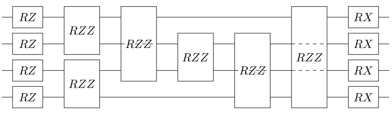
Figure 1: Typical quantum circuit structure for a single layer when implementing DAQC for a 4-qubit QUBO problem. Rotation angles are not displayed for clarity. The circuit is all-to-all connected since each qubit interacts with every other qubit through $R_{ZZ}$ gates. The dashed wires plotted over some $R_{ZZ}$ gates denote wires that are not affected by the gate.

II.3 Challenges from Optimization Perspective

From the optimization point of view, each additional variable $y_{k}^{(i)}$ doubles the search space. Hence, the size of the search space increases exponentially with respect to the number of additional variables. In addition, the energy landscape generally becomes more rugged, because flipping the value of $x_{j}$ or $y_{k}^{(i)}$ may lead to high peaks of energy. For example, consider a feasible solution vector ${(x^{*},y^{*})\in\{0,1\}^{n+\sum_{i=1}^{m}M_{i}}}$ such that all penalty terms are zero. If we now flip a single bit $y^{*(i)}_{k}$ for $k\geq 1$, then the penalty term becomes $\gamma_{i}\left(q_{i}^{T}x^{*}-c_{i}-W_{i}\right)^{2}=\gamma_{i}\left(2^{k}\right)^{2}$. This suggests that solutions differing by a single-bit flip result in exponentially high energy peaks, creating a highly rugged optimization landscape. As a result, the associated optimization problem becomes notably more difficult.

II.4 Concluding Remarks About QUBO

In this section, we have seen that some CO problems, when converted to QUBO, may require significantly more quantum resources. Problems with inequality constraints require additional auxiliary binary variables, and the number of such variables grows logarithmically with the maximum constraint’s value. Quadratic penalties create additional interactions between variables, giving rise to additional 2-qubit $RZZ$ gates. From the optimization perspective, the QUBO formulation has a larger search space, and this makes the problem more difficult for any type of algorithm. Moreover, solutions that are one-bit flip away from the current feasible solution are often infeasible and yield exponentially large penalties.

III Lagrangian dual approach

This study departs from the conventional QUBO approach and investigates the solving of constrained problems using Lagrangian duality theory. We demonstrate the superiority of the proposed approach by comparing it with the QUBO-based approach in the setting of DAQC.

III.1 Lagrangian Duality

We propose a Lagrangian dual DAQC protocol for solving binary combinatorial problems with inequality constraints of the form given in Section II. We also note that the proposed approach generalizes easily to binary quadratic problems with quadratic inequality constraints of the following form:

$$\min_{x}x^{T}Q_{0}x$$

subject to

$$x^{T}Q_{i}x\geq c_{i}\quad\textrm{for}\quad i=1,\ldots,m$$

$$x\in\{0,1\}^{n},$$ (3)

where $Q_{i}\in\mathbb{R}^{n\times n}$ is a symmetric matrix for $i=0,\ldots,m$. The applicability of Lagrangian duality for such problems is investigated in [17]. If $Q_{i}$ is diagonal for $i=0,\ldots,m$, then Section III.1 is equivalent to Section II due the relation $x_{i}^{2}=x_{i}$. Therefore, the formulation in Section III.1 covers a wide range of linear and quadratically constrained and unconstrained combinatorial problems.

We address the QUBO issues discussed in previous sections by using Lagrangian relaxation which is often used in classical optimization. The Lagrangian dual problem corresponding to the primal constrained problem Section II is

$$\max\limits_{\lambda\in\mathbb{R}^{m}_{+}}\;\min\limits_{x\in\{0,1\}^{n}}\left(q_{0}^{t}x+\sum_{i=1}^{m}\lambda_{i}\left(c_{i}-q_{i}^{T}x\right)\right),$$ (4)

where $\lambda_{i}\geq 0$ for $i=1,...,m$ are non-negative Lagrange multipliers. Generally, weak duality holds. That is, if $(x^{*},\lambda^{*})$ is an optimal dual pair and $D^{*}$ is the corresponding objective function value of Eq. 4, then $D^{*}\leq P^{*}$ where $P^{*}$ is the optimal objective function value of the primal problem defined in Section II. For $x^{*}$ to be an optimal solution to the primal problem [Section II], it must be feasible and satisfy the complementary slackness condition $\sum_{i=1}^{m}\lambda_{i}^{*}(c_{i}-q_{i}^{T}x^{*})=0$ [25]. Whenever this condition holds, the duality gap is zero, that is, $D^{*}=P^{*}$, and $x^{*}$ is an optimal solution to the primal problem. If $x^{*}$ is feasible but the complementary slackness is not satisfied, then $\sum_{i=1}^{m}\lambda_{i}^{*}(q_{i}^{T}x^{*}-c_{i})>0$, and we call $x^{*}$ an $\epsilon$-optimal solution to the primal problem with $\epsilon=\sum_{i=1}^{m}\lambda_{i}(q_{i}^{T}x^{*}-c_{i})$ [25]. The value of $\epsilon$ indicates how close $x^{*}$ is to the optimal solution to the primal problem. Therefore, the Lagrangian relaxation can yield optimal or near-optimal solutions to the primal problem. Unlike QUBO, the formulation Eq. 4 neither requires auxiliary variables nor does it involve squared penalty terms. As a result, it permits significantly more efficient quantum circuits as demonstrated in Section IV.

In the context of quantum optimization, the Lagrangian relaxation allows finding the optimal or $\epsilon$-optimal solution to the primal problem by repeated execution of a pre-tuned LD-DAQC circuit followed by measurements; the associated algorithm is presented in Section IV. Our numerical experiments discussed in Section VI.4 suggest that the optimal solution is often contained in the measured sample. Indeed, the optimal solution is measured frequently enough to outperform the traditional QUBO-based approaches.

Since our approach is based on adiabatic evolution in time, we may generalize the Lagrange multipliers $\lambda_{i}$ to time-dependent functions $\lambda_{i}(t)\geq 0$ for $i=1,...,m$ and $t\in[0,T]$. This allows enhanced control over the constraint terms during the adiabatic evolution. Hence, we now define the generalized time-dependent Lagrangian dual by

$$\min\limits_{x\in\{0,1\}^{n}}\left(x^{T}Q_{0}x+\sum_{i=1}^{m}\lambda_{i}(t)\left(c_{i}-x^{T}Q_{i}x\right)\right).$$ (5)

A comprehensive discussion of the time-dependent $\lambda_{i}(t)$ will be undertaken in Section IV.2.

III.2 Lagrangian Dual Adiabatic Quantum Computation

In this section, we use the Lagrangian relaxation in Eq. 4 or the time-dependent Lagrangian dual function of Eq. 5 to construct an efficient LD-DAQC circuit. First, we recast Eq. 5 as a problem of finding the ground state of a Hamiltonian. This is achieved by substituting each variable $x_{j}$ with a spin variable $s_{j}$ using the identity $x_{j}=(1-s_{j})/2$. Then, each variable $s_{j}$ is substituted with the Pauli-Z operator $Z_{j}$ which has eigenvalues $+1$ and $-1$. This substitution relates an abstract binary variable $x_{j}\in\{0,1\}$ with the eigenvalues of the quantum mechanical spin observable and turns the function in Eq. 5 into a Hamiltonian that we denote as $H_{\text{P}}(t)$. Here, the problem Hamiltonian becomes explicitly time-dependent, because $\lambda_{i}(t)$ depends on time.

We use DAQC to find the ground state of $H_{\text{P}}(t)$. For this purpose, we need an initial Hamiltonian $H_{\text{init}}$ whose ground state is known and can be easily prepared in constant time. A typical initial Hamiltonian is the transverse-field operator $H_{\text{init}}=-\sum_{i}^{n}X_{i}$. The adiabatic evolution is achieved by gradually mixing the initial and problem Hamiltonians according to the relation

$$H(t)=\left(1-s(t)\right)H_{\text{init}}+s(t)H_{\text{P}}(t).$$ (6)

In this equation, $s(t)\in[0,1]$ for $t\in[0,T]$ specifies an adiabatic schedule with the requirements $s(0)=0$ and $s(T)=1$. The system is initially prepared in the lowest-energy eigenstate (ground state) of $H(0)=H_{\text{init}}$. Then, according to the adiabatic theorem [26, 27], a sufficiently slow transition from $H_{\text{init}}$ to $H_{\text{P}}(t)$ guarantees that the system remains arbitrarily close to the instantaneous ground state of $H(t)$ and thus evolves into the ground state of $H_{\text{P}}$ at the end of the schedule at $t=T$.

It is important to note that, whenever Eq. 5 is linear, such as in the knapsack problem that we study in Section V, the objective function does not have quadratic terms of the form $x_{i}x_{j}$. In this case, the resulting quantum circuit does not have 2-qubit $RZZ$ gates and, consequently, it cannot create entanglement. Yet, it is known that entanglement is a necessary resource for quantum speedup [28, 29]. To introduce entangling operations, we add quadratic terms without modifying the formulation of the optimization problem. Clearly, any addition of quadratic terms $x_{i}x_{j}$ to Eq. 5 would change the optimization problem to a different optimization problem; similarly, any addition of operators $Z_{i}Z_{j}$ to $H_{\text{P}}(t)$ would change the problem Hamiltonian such that it is no longer equivalent to the problem in Eq. 5. Our solution is to use a different initial Hamiltonian with quadratic terms that do not commute with the $Z_{i}$ or $Z_{i}Z_{j}$ terms in $H_{\text{P}}(t)$. More specifically, we consider the 2-local Hamiltonian referred to as the $ZZXX$ universal Hamiltonian [30] which has the form:

$$H_{ZZXX} =\sum_{i}h_{i}X_{i}+\sum_{i}\Delta_{i}Z_{i}$$

$$+\sum_{i,j}K_{i,j}X_{i}X_{j}+\sum_{i,j}J_{i,j}Z_{i}Z_{j}.$$ (7)

We identify the terms $\sum_{i}h_{i}X_{i}$ and $\sum_{i,j}K_{i,j}X_{i}X_{j}$ with the new initial Hamiltonian, whereas the rest of the terms are used to represent the problem Hamiltonian. Therefore, 2-qubit interactions are introduced through the use of the terms in $\sum_{i,j}K_{i,j}X_{i}X_{j}$ of the 2-local $ZZXX$ Hamiltonian. We hypothesize that a specific choice of the coefficients $K_{i,j}$ can introduce correlations between qubits that could potentially yield better performance. Generally, the choice of $K_{i,j}$ can be informed by quantum hardware architecture or by the structure of a CO problem. In this study, we choose the coupling coefficients $K_{i,j}$ such that they form a chain with a periodic boundary condition. Specifically, we use the mixing Hamiltonian

$$H_{\text{init}}=-\sum_{i=1}^{n}X_{i}-\sum_{i=1}^{n}X_{i}X_{i+1}\,,$$ (8)

where we define $n+1:=1$. As shown in Section IV, this choice yields a highly parallelizable circuit with circuit depth independent of the problem size $n$.

Note that, if the problem in Eq. 5 is linear, the associated Lagrangian dual is also linear. It follows that $H_{\text{P}}$ is a 1-local Hamiltonian and $H_{\text{init}}$ in Eq. 8 is a 2-local Hamiltonian with a user-provided qubit coupling. It is also possible to set $K_{i,j}=0$ for all $i,j$. Then the Hamiltonian $H(t)$ becomes a 1-local Hamiltonian, because both $H_{\text{init}}$ and $H_{\text{P}}$ are 1-local Hamiltonians. In this particular case, the simulation of evolution generated by $H(t)$ is in the complexity class P, and the corresponding LD-DAQC circuit can be efficiently simulated classically. Therefore, by appropriately selecting the coefficients $K_{i,j}$, we can explore two distinct heuristics: one that leverages entanglement to achieve a potential quantum speedup, and another that uses Hamiltonian 1-locality to obtain an efficient classical heuristic.

IV LD-DAQC for Linear Problems

In this section, we construct an efficient quantum circuit which, unlike circuits derived from the QUBO approach, is substantially more parallelizable, does not require auxiliary qubits, and requires only nearest-neighbour qubit connectivity.

To find the optimal solution to Section II, we start the development of our quantum circuit by approximating the problem in Section II using the time-dependent Lagrangian relaxation:

$$\min\limits_{x\in\{0,1\}^{n}}\left(q_{0}^{t}x+\sum_{i=1}^{m}\lambda_{i}(t)\left(c_{i}-q_{i}^{T}x\right)\right).$$ (9)

Generally, $\lambda_{i}(t)$ can be a parametrized function of time as in Section IV.2, and its parameters are determined through hyperparameter tuning as explained in Section VI. In the special case when $\lambda_{i}(t)\equiv\lambda_{i}$ is time-independent for all $i$, then this objective function is convex in $\lambda_{i}$. The optimal $\lambda_{i}^{*}$ for a Lagrangian dual problem in Eq. 4 can be estimated to an arbitrary error $\epsilon>0$ in $O(\epsilon^{-2})$ iterations using the subgradient method [31].

Next, we recast Eq. 9 as a problem of finding the ground state of a Hamiltonian. By substituting binary variables $x_{j}$ with spin variables $s_{j}$ according to the relation $x_{j}=(1-s_{j})/2$ and introducing Pauli-Z operators $Z_{j}$ we obtain the problem Hamiltonian $H_{\text{P}}(t)$ which is linear in $Z_{j}$. Dropping all constant terms in $H_{\text{P}}(t)$ yields

$$H_{\text{P}}(t)=\sum_{j=1}^{n}\left(-q_{0j}+\sum_{i=1}^{m}\lambda_{i}(t)q_{ij}\right)Z_{j}.$$ (10)

Combining $H_{\text{P}}(t)$ with $H_{\text{init}}$ in Eq. 8 yields the total Hamiltonian

$$H(t)= \left(1-s(t)\right)\left(-\sum_{j=1}^{n}X_{i}-\sum_{j=1}^{n}X_{j}X_{j+1}\right)$$

$$+ s(t)\sum_{j=1}^{n}\left(-q_{0j}+\sum_{i=1}^{m}\lambda_{i}(t)q_{ij}\right)Z_{j},\ t\in[0,T],$$ (11)

where $s(t)$ is an adiabatic schedule.

Given the initial ground state $\ket{\psi(0)}=\ket{+}^{\otimes n}$ of $H_{\text{init}}$, the evolved state $\ket{\psi(t)}$ can be expressed as $\ket{\psi(t)}=U(t,0)\ket{\psi(0)}$, where $U(t,0)$ is the time evolution operator which satisfies the Schrödinger equation, $\mathrm{i}dU(t,0)/dt=H(t)U(t,0)$. In order to construct the LD-DAQC circuit, we subdivide the time interval $[0,T]$ into $p$ subintervals of length ${\Delta t=T/p}$. Then the time evolution operator is given by

$$U(T,0)=\lim_{p\rightarrow\infty}\prod^{p}_{k=0}\exp\left\{-\mathrm{i}\Delta tH(\Delta tk)\right\}.$$ (12)

To approximate Eq. 12, we choose $p$ to be finite and apply the established first-order Trotterization formula. This yields a $p$-layered LD-DAQC circuit,

$$\hat{U}(T,0)=\prod^{p}_{k=1}\exp\left\{-\mathrm{i}c_{k}H_{\text{init}}\right\}\exp\left\{-\mathrm{i}b_{k}H_{\text{P}}(\Delta tk)\right\},$$ (13)

with $H_{\text{init}}$ and $H_{\text{P}}(t)$ given by Eq. 8 and Eq. 10, respectively, and $c_{k},b_{k}$ defined as

$$c_{k} =\left(1-s(k\Delta t)\right)\Delta t,$$

$$b_{k} =s(k\Delta t)\Delta t.$$ (14)

It was suggested in [8] to normalize the Hamiltonians $H_{\text{init}}$ and $H_{\text{P}}$ by their corresponding Frobenius norms. Therefore, we substitute $c_{k}$ and $b_{k}$ defined in Section IV with

$$\gamma_{k} =\frac{c_{k}}{||H_{\text{init}}||},$$

$$\beta_{k} =\frac{b_{k}}{||H_{\text{P}}||}.$$ (15)

Empirically, we verified that Frobenius normalization yields a well-performing schedule. However, the theoretical basis for this is not understood.

We now examine the structure of the resulting circuit $\hat{U}(T,0)$ given in Eq. 13. For any layer $k\in\{1,...,p\}$ consider the unitary matrix given by the initial Hamiltonian. Due to the commutativity of $X_{i}$ and $X_{i}X_{j}$ the matrix can be written as

$$\exp\left\{-\mathrm{i}\gamma_{k}H_{\text{\text{init}}}\right\}=\prod_{j=1}^{n}\exp\left\{\mathrm{i}\gamma_{k}X_{j}X_{j+1}\right\}\prod_{j=1}^{n}\exp\left\{\mathrm{i}\gamma_{k}X_{j}\right\}.$$ (16)

The unitary matrix given by the problem Hamiltonian can be written as

$$\exp \left\{-\mathrm{i}\beta_{k}H_{\text{P}}(\Delta tk)\right\}=$$

$$\prod_{j=1}^{n}\exp\left\{-\mathrm{i}\beta_{k}\left(-q_{0j}+\sum_{i=1}^{m}\lambda_{i}(\Delta tk)q_{ij}\right)Z_{j}\right\}.$$ (17)

We note that the Lagrange multiplier $\lambda_{i}(\Delta tk)$ in Section IV contributes to the angle of rotation and depends on the time step $\Delta tk$. For any $k$, the unitary matrices in Section IV can be represented by 1-qubit $RZ$ gates. Conversly, the unitary matrices given in Eq. 16 can be represented by 1-qubit $RX$ gates and 2-qubit $RXX$ gates. Hence, the LD-DAQC circuit $\hat{U}(T,0)$ can be expressed as follows:

$$\hat{U}(T,0)= \prod_{k=1}^{p}\prod_{j=1}^{n}RXX_{j,j+1}(-2\gamma_{k})$$

$$\times \prod_{j=1}^{n}RX_{j}(-2\gamma_{k})$$

$$\times \prod_{j=1}^{n}RZ_{j}\left(2\beta_{k}\left(-q_{0j}+\sum_{i=1}^{m}\lambda_{i}(\Delta tk)q_{ij}\right)\right).$$ (18)

The structure of the $k$-th layer of $\hat{U}(T,0)$ is illustrated in Fig. 2.

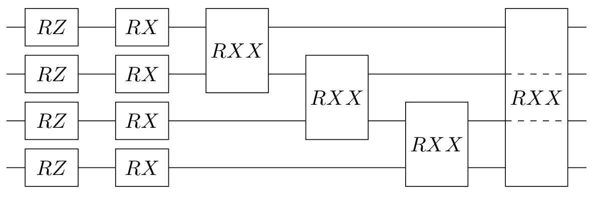
Figure 2: The $k$-th layer of the 4-qubit LD-DAQC. Rotation angles are not displayed for clarity.

The resulting circuit is extremely parallelizable and hence has a short circuit depth. All $RZ$ gates can be applied in a single time step. Similarly, all $RX$ gates can be applied in a single time step. All $RXX$ gates can be applied in 2 time steps if $n$ is even, and in 3 time steps if $n$ is odd. Hence, the circuit depth complexity is $O(p)$; that is, the circuit depth depends only on the parameter $p$, but it does not depend on the problem size; for further discussion, see Appendix A. Moreover, due to the choice of the coefficients $K_{i,j}$ in $H_{\text{\text{init}}}$ in Eq. 8, the resulting circuit features only nearest-neighbour qubit connectivity. Finally, this circuit construction does not involve auxiliary qubits.

IV.1 DAQC Scheduling

In this section, we give an explicit description of the adiabatic schedule $s(t)$ used in this study. Ideally, we would like to have a single adiabatic schedule that maximizes the probability of observing optimal solutions to multiple problem instances of the same problem class. A problem class can be, for example, an $n$-variable knapsack problem or an $n$-variable travelling salesperson problem.

We adapt the QA scheduling presented in [4]. For better control of the curvature of the schedule function, we use a cubic polynomial approximation proposed in [8]. The general form is given as follows

$$s(t;a,T)=\frac{t}{T}+a\cdot\frac{t}{T}\left(\frac{t}{T}-\frac{1}{2}\right)\left(\frac{t}{T}-1\right).$$ (19)

The parameters $a$ and $T$ define the slope and the evolution time, respectively. The goal is to determine optimal parameters $a^{*}$ and $T^{*}$ that maximize the probability of observing an optimal solution for similar problem instance of the same size. This is usually achieved by using a “training” set of problem instances of size $n$ and performing a Random Search optimization [32] on $a$ and $T$ to directly minimize the median of time-to-solution (TTS) metrics (to be defined in Section VI.3) for all problems in the “training” set. Once $a^{*}$ and $T^{*}$ are determined, we can reuse $s(t;a^{*},T^{*})$ across all similar problem instances of size $n$ and achieve a high probability of measuring the optimal solution.

IV.2 Lagrangian Multiplier Scheduling

In this section we discuss the generalized Lagrange multipliers $\lambda_{i}(t)$ for $i=1,...,m$ and $t\in[0,T]$. First, we note that constant $\lambda_{i}$ is a special case of $\lambda_{i}(t)$. Most combinatorial problems have no notion of time. That is, the problem formulation and its solution are time-independent. Therefore, it makes sense to use Lagrange multipliers that are also constant. However, when using the DAQC approach, the solution to a problem is gradually obtained during the adiabatic evolution. The inherent time-dependence of the adiabatic process can be used to control the strength of the Lagrange multipliers. For example, it is possible to delay the introduction of some difficult constraints allowing the process to start with an easier problem. Alternatively, soft constraints, which are preferred but do not necessarily have to be fulfilled, can also be scheduled to appear towards the end of the evolution. In this study, we define the time-dependent Lagrangian multipliers in terms of the modified schedule in Eq. 19:

$$\lambda_{i}(t;o_{i},\gamma_{i},a_{i}):=\gamma_{i}\cdot s(t-o_{i};a_{i},T)\cdot\mathbb{1}_{o_{i}<t}(t)$$

$$\textrm{ for }\ i=1,\ldots,m.$$ (20)

In the equation above, $\gamma_{i}>0$ is the weight of the schedule, $o_{i}\in[-T,T]$ is the time offset, $a_{i}$ is a schedule slope coefficient, and $\mathbb{1}_{o_{i}<t}(t)$ is an indicator function such that $\mathbb{1}_{o_{i}<t}(t)=1$ for $o_{i}<t$ and $\mathbb{1}_{o_{i}<t}(t)=0$ otherwise. Setting $o_{i}=T/2$ introduces the constraint $i$ in the middle of the adiabatic process, whereas $o_{i}=T$ is equivalent to ignoring the constraint completely as $\lambda_{i}(t;o_{i},\gamma_{i},a_{i})=0$ for all $t\in[0,T]$.

V Numerical experiments

This section presents a well-known linear problem that is a special case of the general formulation in Section II, and compares numerical results obtained by QUBO-DAQC and LD-DAQC circuits for that problem. We will see that the proposed LD-DAQC significantly outperforms the canonical QUBO-based circuit.

V.1 Knapsack Problem

For our benchmarking study, we use a well-known optimization problem called 1D 0–1 knapsack problem (KP) [33] as the reference problem for comparison. A KP is an NP-complete linear problem that can be formulated as a special case of Section II in which $m=1$. In combinatorial optimization, a KP requires selecting the most valuable items to fit into a knapsack without exceeding its capacity. This problem has diverse industrial applications, including resource allocation, scheduling, and inventory management.

We derive a KP from the general canonical formulation given in Section II. Suppose we have a KP with $n$ items. Let $v_{j},w_{j}\in\mathbb{N}$ denote the $j$th item’s value and weight respectively and $c\in\mathbb{N}$ is the knapsack capacity. By setting the entries $q_{0,j}=-v_{j}$, $q_{1,j}=-w_{j}$ for all $j=1,\dots,n$ and $c_{1}=-c$ we obtain the canonical formulation of the $n$-variable KP

$$\textrm{max}\sum_{j=1}^{n}v_{j}x_{j}$$

subject to

$$\sum_{j=1}^{n}w_{j}x_{j}\leq c$$

$$x\in\{0,1\}^{n}.$$ (21)

Our choice of this problem is based on several considerations. First, a KP is a typical representative of NP-complete constrained binary linear problems. Second, as we will show below, trying to solve the KP in the quantum setting by the means of adiabatic computation with the canonical QUBO reformulation Section II results in a prohibitively costly circuit which requires all-to-all connectivity and additional auxiliary qubits whose number grows logarithmically with the constraint bound $c$. Therefore, a KP is a good representative of CO problems that challenge currently available quantum optimization approaches. Developing a quantum protocol that successfully solves the KP means that the majority of other binary linear programs with inequality and equality constraints can also be successfully solved by the same protocol.

V.2 LD-DAQC Circuit

We start the development of our LD-DAQC by approximating the problem in Eq. 21 using the Lagrangian dual given below:

$$\min_{x\in\{0,1\}^{n}}\left(-\sum_{j=1}^{n}v_{j}x_{j}+\lambda(t)\left(\sum_{j=1}^{n}w_{j}x_{j}-c\right)\right).$$ (22)

As before, if we let $\lambda(t)\equiv\lambda$ to be independent of time, then the problem Eq. 9 is convex in $\lambda$. Note that Eq. 22 is a particular case of the general formulation in Eq. 9. From the general LD-DAQC given in Section IV it is straightforward to deduce the structure of the LD-DAQC for the KP; we set $m=1$, $q_{0j}=-v_{j}$ and $q_{1j}=w_{j}$. This gives the LD-DAQC for the KP.

V.3 QUBO-DAQC Circuit

To derive a QUBO circuit for KP, we first reformulate the KP in Eq. 21 as a QUBO problem. For this we use the general QUBO formulation given in Section II. In this case, we get:

$$\min_{x,y}\left(-\sum_{j=1}^{n}v_{j}x_{j}+\gamma\left(\sum_{j=1}^{n}w_{j}x_{j}-W\right)^{2}\right)$$

subject to

$$W=\sum_{k=0}^{\lfloor\log_{2}(c)\rfloor-1}2^{k}y_{k}+(c+1-2^{\lfloor\log_{2}(c)\rfloor})y_{\lfloor\log_{2}(c)\rfloor}$$

$$y\in\{0,1\}^{\lfloor\log_{2}(c)\rfloor+1}$$

$$x\in\{0,1\}^{n},$$ (23)

where $\gamma$ is a penalty multiplier and $c$ is the constraint inequality bound. We note that the number of additional auxiliary binary variables $y_{k}$ grows as $O(\log_{2}c)$. Since $w_{j}>0$ for $j=1,\ldots,n$, from the discussion in Section II.2, it is clear that the squared penalty term introduces $\binom{n+\log_{2}(c)+1}{2}$ pairwise interactions between every qubit in each layer of the circuit. That is, each layer of the circuit will have $\binom{n+\log_{2}(c)+1}{2}$ 2-qubit $RZZ$ gates. Therefore, each layer of the circuit is all-to-all connected. Due to this, the circuit is poorly parallelizable and has circuit depth $O\left(p(n+\log_{2}c)\right)$ – for further information see Appendix A. Therefore, the circuit depth depends on the problem size $n$, the value of the constraint bound $c$ and the number of layers $p$. For example, if the constraint bound $c\geq 2^{2n}$, then the number of auxiliary qubits is at least double of the problem size $n$. This means even relatively small knapsack problems may be very challenging for quantum optimization.

One might attempt to decrease the number of auxiliary qubits by scaling down the coefficients $w_{j}$ and the constraint bound $c$ by dividing both sides of the inequality constraint in Eq. 21 by some constant $z\in\mathbb{N}$. However, this often leads to fractional values, i.e., $\sum_{j=1}^{n}w_{j}x_{j}/z\in\mathbb{Q}\setminus\mathbb{N}$ for some $x\in\{0,1\}^{n}$. This implies that the slack variable $W$ must be able to approximate the rational $\sum_{j=1}^{n}w_{j}x_{j}/z$ for all feasible $x$. Hence, the binary expansion of $W$ must include additional auxiliary binary variables that represent a fractional part. Therefore, in the presence of inequality constraints, it is practically impossible not to have auxiliary qubits.

VI Experimental setup and Results

In this section, we discuss the computational setup used in the experiment, present procedures used to generate multiple KP datasets, and various metrics used for our analysis. We compare the performance of QUBO-DAQC and LD-DAQC and demonstrate the superiority of the latter.

VI.1 Hardware Setup

The experiment involved very large LD-DAQC and QUBO-DAQC circuits, some of which had 100 Trotter layers, 20 qubits and all-to-all connectivity. Executing such deep circuits on a quantum computer would require fault-tolerant architectures whose development is still in its infancy. Therefore, all quantum computations were simulated on classical hardware. This was a large-scale experiment which pushed quantum simulation to its limits. To compute the experimental results presented in this paper, we used over 240 hours of 64-core, 32-core and 16-core CPUs and over 200 GB of RAM on the Google Cloud Platform (GCP). Especially demanding QUBO-based quantum circuits whose single execution required at least two weeks of CPU time on the GCP were executed on Nvidia’s A100 High-Performance Computing server, reducing the computation time from weeks to several hours. In this experiment, more than 2,000 optimization problem instances were generated and solved using quantum simulation. The correctness of simulation results was verified with Google’s classical optimization solvers: OR-Tools Linear Optimization Solver and OR-Tools Brute Force Solver [34].

VI.2 Generation of Random Instances

We create two different types of test supersets of KPs:

1. The purpose of the Superset 1 is to examine performance scaling with respect to the problem size $n$. Thus, for each $n=5,6,\ldots,15$ we generate 100 KP instances with integer coefficients $v_{i},w_{i}$ distributed according to the uniform probability distribution with bounds $1$ and $10$. That is, integers $v_{i},w_{i}\sim U(1,10)$. The capacity $c$ is a function of random variables $w_{i}$ and it is defined as $c=\lfloor\sum_{i}w_{i}/2\rfloor$.

2. The purpose of the Superset 2 is to examine performance scaling with respect to the scale of the coefficients $v_{i}$ and $w_{i}$ while $n$ is fixed. For a fixed ${n=11}$ and each $C=10,20,30,\ldots,100$ we generate 100 problem instances such that ${v_{i},w_{i}\sim U(1,C)}$. Hence, there are 10 datasets each containing instances of size $n=11$ but with coefficients $v_{i},w_{i}$ whose range is incremented by 10 units in each dataset.

Two additional training supersets of data were also created with the same setup as above. The training supersets were only used for hyperparameter tuning of $p$, $T$, $a$ specifying the DAQC scheduling function in Eq. 19 and $\gamma_{1}$, $o_{1}$ and $a_{1}$ specifying the Lagrange multiplier scheduling function in Section IV.2. To identify the best parameters for each $n$, we employ Random Search [32] across the parameter space, aiming to minimize the median TTS which we introduce as our key performance metrics in the next section.

VI.3 Circuit Scaling: LD-DAQC vs. QUBO-DAQC

In order to evaluate the performance of QUBO-DAQC and LD-DAQC on the test datasets we use the $R_{99}$ and the time-to-solution (TTS) metrics. Let a parameter sequence $\theta=\{(\gamma_{k},\beta_{k})\}_{k=1}^{p}$ defined in Section IV be given. Then $R_{99}(\theta)$ is the number of “shots” (executions of the quantum circuit followed by measurements) that must be performed to ensure a $99\%$ probability of successfully observing the ground state of the problem Hamiltonian $H_{\text{P}}$ for a given circuit parametrization $\theta$ at least once. It is defined as (see, e.g., [8])

$$R_{99}(\theta):=\frac{\log(0.01)}{\log(1-P(\theta))},$$ (24)

where $P(\theta)$ denotes the probability of measuring the optimal solution given the parametrization $\theta$. The TTS denotes the expected computation time required to find an optimal solution for a particular problem instance with $99\%$ confidence. It is defined by

$$\textrm{TTS}(\theta)=R_{99}(\theta)\cdot t_{\text{ss}}\,,$$ (25)

where $t_{\text{ss}}$ denotes the runtime for a single shot.

In order to approximate $t_{\text{ss}}$, we make the following assumptions:

1. A quantum processor performs any single-qubit and two-qubit gate operations in 10 and 20 nanoseconds, respectively; this is in accordance with current state-of-the-art realizations of superconducting quantum hardware technologies, see e.g. [35].

2. Gate operations may be performed simultaneously if they do not act on the same qubit.

3. All components of the circuit are noise-free; hence there is no overhead for quantum error correction or fault-tolerant quantum computation.

Then, as shown in Appendix A, a $p$-layered LD-DAQC circuit has the following runtime dependence on $p$ and $n$:

$$t_{\text{ss}}=\begin{cases}50p\,,&\;\text{if }\,n\ \textrm{ is even}\\ 70p\,,&\;\text{if }\,n\ \textrm{ is odd}\;.\end{cases}$$ (26)

Note that, for LD-DAQC circuits, $t_{\text{ss}}$ does not explicitly scale with the problem size $n$. In contrast, a $p$-layered QUBO-DAQC circuit has the following runtime dependence on $p$, the problem size $n$, and the constraint bound $c$:

$$t_{\text{ss}}=\begin{cases}20p\left(n+\log_{2}c\right),&\text{if }\,n+\log_{2}c\textrm{ is even}\\ 20p\left(n+\log_{2}c+1\right),&\text{if }\,n+\log_{2}c\textrm{ is odd}\;.\end{cases}$$ (27)

VI.4 Experiment Results

In this section, we analyze the optimal resource requirements in terms of the number of Trotter layers $p$, evolution time $T$, and the number of qubits for both circuit types to achieve comparable $R_{99}$ values across all problem sizes. The numerical experiments demonstrate that the LD-DAQC circuits require quadratically fewer resources than QUBO-DAQC circuits while attaining comparable $R_{99}$ values for both approaches. Importantly, we show that $R_{99}$ for LD-DAQC circuits remains unaffected by the expansion in the range of problem coefficients $w_{i}$ and $v_{i}$. In contrast, QUBO-DAQC circuits display a polylogarithmic growth in $R_{99}$ when the range of coefficients $w_{i}$ is increased.

VI.4.1 Linear Resouce Scaling of LD-DAQC

Fig. 3 displays the scaling of the optimal mean number of Trotter layers $p$ and the optimal evolution time $T$ with respect to the problem size. The LD-DAQC circuits have a linear scaling, whereas the QUBO-DAQC circuits have a quadratic scaling for both $p$ and $T$.

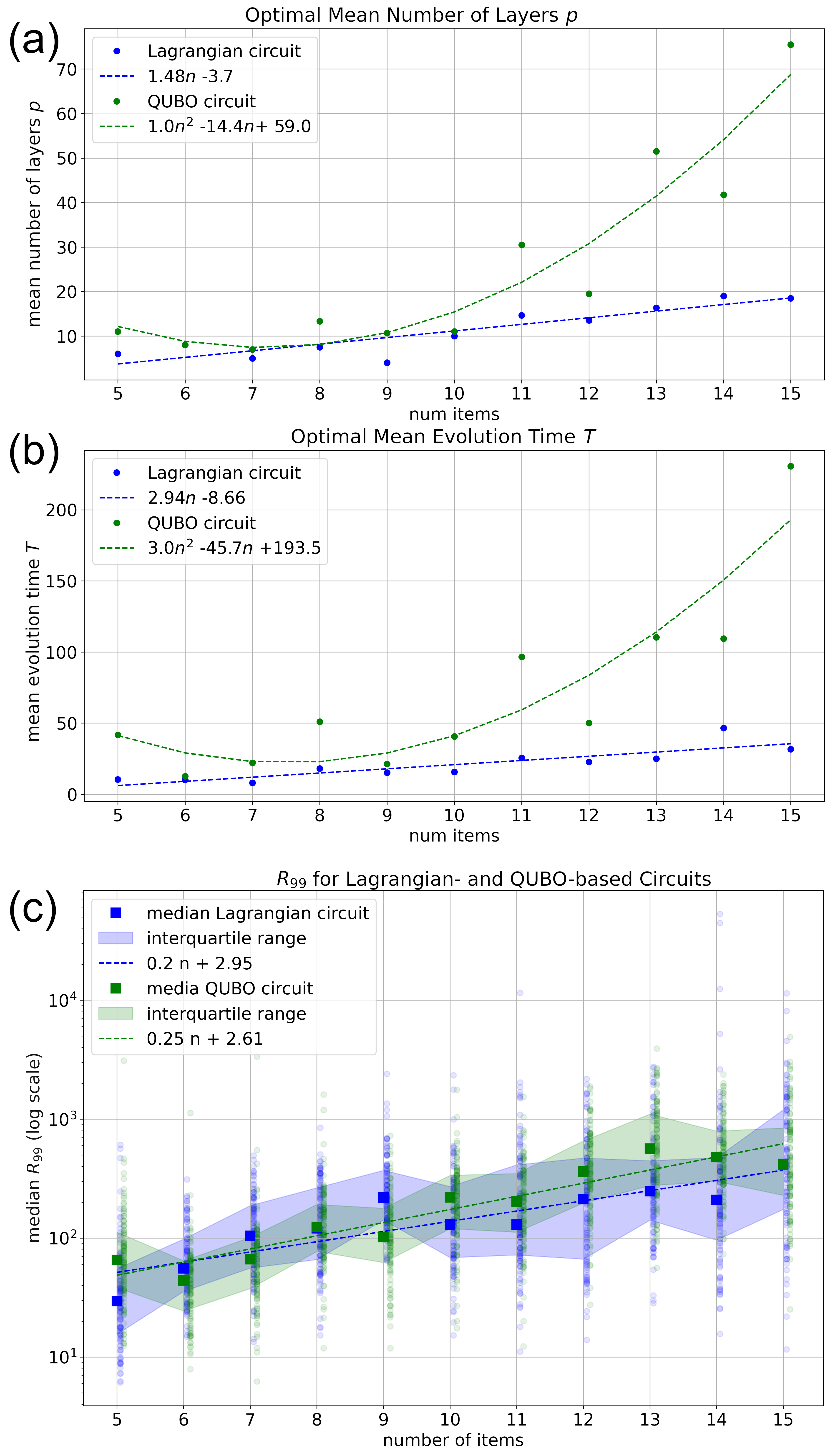
Figure 3: Scaling of the optimal number of Trotter layers $p$, optimal evolution time $T$, and $R_{99}$, with respect to the problem size (number of items) for LD-DAQC (blue) and QUBO-DAQC (green) circuits. (a) The optimal mean depth $p$ scales linearly for LD-DAQC, whereas it exhibits a quadratic growth for the QUBO-DAQC circuit. (b) The optimal mean evolution time $T$ also scales linearly for LD-DAQC, whereas it exhibits a quadratic growth for the QUBO-DAQC circuit. (c) $R_{99}$ for LD-DAQC and QUBO-DAQC circuits assuming optimal parameters $p$ and $T$, respectively. Given optimal parameters for each approach, the corresponding circuits have a comparable $R_{99}$ exhibiting an exponential scaling with respect to the problem size.

This difference becomes even more critical if we take into account the overhead costs associated with quantum error correction (QEC) and the realization of fault-tolerant quantum computation (FTQC) schemes that become necessary for deep circuits implemented on noisy real-world devices. Deeper circuits are much more vulnerable to noise, necessitating greater QEC and FTQC overhead costs, which have been neglected in our analysis because we aimed at comparing optimistic lower bounds for the two approaches.

VI.4.2 Invariance of LD-DAQC to Coefficient Range Increase

Recall that whenever a combinatorial optimization problem includes inequality constraints, additional qubits are required to account for encoding the slack variables. It has been established that the count of these additional qubits scales logarithmically with the constraint bounds. Employing Superset 2, we examine the performance scaling on fixed-size KP datasets ($n=11$), but with an increasing value range for the coefficients $v_{i}$ and $w_{i}$. In Fig. 4, we illustrate the scaling behaviour of $R_{99}$ for both circuit categories, each maintaining fixed parametrization and layer counts across all datasets. It is clear that for LD-DAQC circuits, $R_{99}$ remains invariant to the increase of the range of $v_{i}$ and $w_{i}$, exhibiting consistent $R_{99}$ throughout all datasets in Superset 2. In contrast, QUBO-DAQC circuits manifest a quadratically logarithmic growth in $R_{99}$. This observed scaling can be attributed to the logarithmic increase in auxiliary variables intrinsic to QUBO reformulations of problems containing inequality constraints.

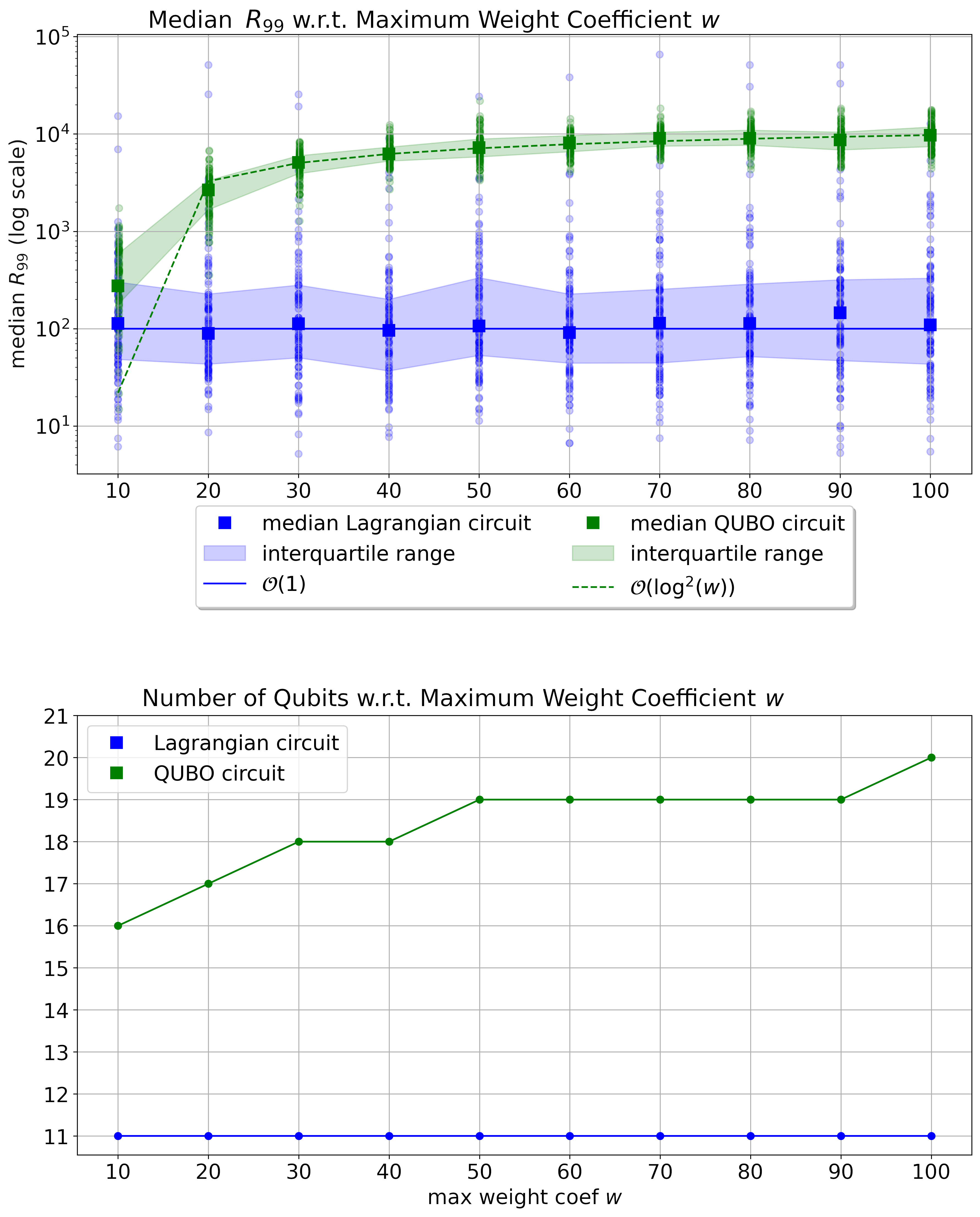
Figure 4: Scaling of $R_{99}$ and the number of qubits with respect to the maximum weight coefficient (knapsack capacity bound) for LD-DAQC circuits (blue) and QUBO-DAQC circuits (green). A single fixed parametrization was used for all datasets, that is, $p$, $T$ and $s(t)$ are fixed across all datasets.

The observed scaling behavior in relation to the expanding range of coefficients $v_{i}$ and $w_{i}$ underscores a pivotal observation about the TTS scaling of LD-DAQC and QUBO-DAQC circuits. Given the quadratically logarithmic growth of QUBO-DAQC in $R_{99}$ with respect to the increasing range of $w_{i}$, as shown in Fig. 4, we conclude that the TTS disparity between the two circuit types can be arbitrarily magnified by selecting KP problems with larger capacity bounds for the weights $w_{i}$. For instance, calculating the TTS difference at $n=15$ with a moderately realistic item weight distribution $w_{i}\sim U(1,1000)$, the median TTS difference would ascend to a minimum of two orders of magnitude. Nevertheless, even for $n=15$ with $w_{i}\sim U(1,10)$, we are swiftly approaching the computational limits for simulating outcomes with QUBO-based circuits.

VII Conclusion

In this study, we analyze two approaches to solving combinatorial optimization problems with constraints within the framework of circuit-model quantum optimization based on adiabatic evolution. We argue that the prevalent traditional approach of recasting a constrained optimization problem into a quadratic Ising model using the QUBO formalism is highly inefficient; moreover, in addition to being costly in terms of the required computational resources, it often results in ill-behaved optimization landscapes. To address these challenges, we develop an alternative adiabatic quantum computation scheme that is based on the principle of Lagrangian duality from classical theory of optimization. Using quantum circuits obtained by a Trotterized approximation to adiabatic evolution to realize a discrete implementation of adiabatic quantum computation (DAQC), we show that a DAQC scheme based on Lagrangian dual can be much more efficient than a DAQC scheme based on the QUBO approach. In particular, the Lagrangian dual approach results in significantly lower circuit connectivity and circuit depth compared to the latter. Furthermore, it also eliminates the need for logarithmic overheads in qubit count due to constraint bounds. We have conducted a numerical benchmarking study which suggests that the proposed Lagrangian dual DAQC circuits yield a quadratic improvement over QUBO-based circuits in terms of adiabatic evolution time and circuit depth, while achieving a comparable performance in solving a given constrained optimization problem. We further found that while LD-DAQC’s performance is consistent regardless of a problem’s coefficient values, the QUBO-based approach manifests a polylogarithmic growth in $R_{99}$ as the coefficient value range expands.

While the present study relies on discretized adiabatic scheduling, our proposed methodology is also applicable to variational algorithms and diabatic state preparation schemes, such as QAOA. In particular, the adiabatic schedule can be used as an initial guess and further refined through parameter optimization using a classical optimizer in a feedback loop. Such an approach could potentially further decrease the circuit depth or increase the algorithmic performance in terms of the expected time required to find an optimal solution for a given problem with high confidence.

Future investigations may address the potential for further performance or resource requirements improvements through a clever choice of the coupling terms $K_{i,j}X_{i}X_{j}$ in the mixing Hamiltonian given in Section III.2. For instance, the coefficients $K_{i,j}$ could be suitably chosen to exploit the structure of an optimization problem and its constraints in order to achieve a better performance in finding the optimal feasible solution. The specific choice made in our benchmarking study was motivated by our aim at reducing the circuit depth while allowing the realization of entangling operations for any pair of qubits. Other choices may potentially yield a better algorithmic performance. The concrete values of these coefficients can also account for the connectivity constraints of a given quantum hardware architecture and thus may depend on the choices of an end-user.

Finally, we anticipate that the Lagrangian dual adiabatic quantum computation methodology proposed in the present work could also be applied to the more general framework of mixed-integer programming (MIP) [36, 37, 38]. Indeed, a recent study proposed an approach to MIP based on continuous-variable adiabatic quantum computation (CV-AQC) on a set of bosonic quantum field modes (qumodes) [39]. In that study, inequality constraints were handled by including quadratic penalty terms in the problem Hamiltonian along with additional auxiliary qumodes to encode the slack variables. It would be interesting to investigate if the Lagrangian dual methodology could potentially improve CV-AQC schemes in solving MIP problems with constraints.

VIII Acknowledgements

The authors thank Pooya Ronagh for his critical feedback and suggestions that greatly improved this work. EG would also like to express his gratitude to Ben Adcock for his invaluable guidance, constant support, patience, and immense knowledge throughout the course of this research.

Appendix A Analysis of Runtime Complexity for LD-DAQC and QUBO-DAQC Circuits

Recall that one-qubit gates acting on different qubits can be executed in parallel, whereas any pair of two-qubit gates sharing at least one qubit can only be executed sequentially. As a result, highly parallelizable circuits have shorter runtime and are less prone to accumulation of errors. This section demonstrates the runtime complexity of the Lagrangian- and QUBO-based circuits for a KP. In Section VI.3 we stated that the LD-DAQC circuit’s runtime $t_{\text{ss}}$ is $O(p)$ where $p$ is the number of layers. In contrast, the QUBO-DAQC circuit has runtime complexity $O\left((n+\log_{2}(c))p\right)$ where $n$ is the number of variables in a KP and $c$ is the capacity.

Let us first look at the LD-DAQC circuit given in Eq. 13-Section IV. To show that the runtime $t_{\text{ss}}$ is $O(p)$ it is sufficient to examine any single layer of the circuit illustrated in Fig 2. The $k$th layer has the following form:

$$\prod_{j=1}^{n}\exp\left\{\mathrm{i}\gamma_{k}X_{j}X_{j+1}\right\}\times\prod_{j=1}^{n}\exp\left\{\mathrm{i}\gamma_{k}X_{j}\right\}$$

$$\times\prod_{j=1}^{n}\exp\left\{-\mathrm{i}\beta_{k}\left(v_{j}-\lambda(\Delta tk)w_{j}\right)Z_{j}\right\}.$$ (28)

We claim that the runtime of a single layer $k$ is constant. Intuitively, we can rearrange the gates of the $k$th layer into at most five sublayers such that gates belonging to a sublayer can be applied in parallel. Each sublayer has the runtime $O(1)$. Fig 5 illustrates a 4-qubit $k$th layer of a LD-DAQC circuit and its equivalent rearrangement into four sublayers that can be applied consecutively. For all $j=1,\ldots,n$ the unitary matrix $\exp\left\{\mathrm{i}\gamma_{k}X_{j}\right\}$ represents a one-qubit $RX_{j}$ gate acting on the qubit $j$. Therefore, their product can be applied in parallel in one step. Similarly, the matrix $\exp\left\{-\mathrm{i}\beta_{k}\left(v_{j}-\lambda(\Delta tk)w_{j}\right)Z_{j}\right\}$ represents a one-qubit $RZ_{j}$ gate acting on the qubit $j$. Hence, the product of all $RZ$ gates can be applied in parallel in one step. We conclude that the number of steps required to apply all $RX$ and $RZ$ gates is independent of $n$, i.e., it is constant per layer $k$.

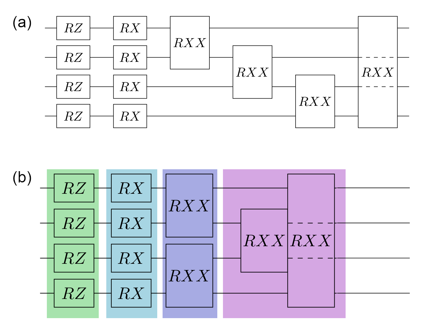
Figure 5: (a) The $k$th layer of the LD-DAQC circuit. By the choice of the coefficients $K_{i,j}$ in Section III.2 we get the initial Hamiltonian Eq. 8, which in turn yields $RXX$ gates with a closed chain-like connectivity. (b) Equivalent rearrangement of the $k$th layer. Gates are partitioned into four sublayers (coloured rectangles). Gates belonging to the same sublayer do not share qubits and can be applied in parallel in a single step. In total it takes four consecutive executions to apply the $k$th layer for any even $n$.

We now examine the two-qubit gates $RXX_{j,j+1}$ given by $\exp\left\{\mathrm{i}\gamma_{k}X_{j}X_{j+1}\right\}$. We note that their product forms a closed chain where the qubit $j$ is connected to the qubit $j+1$, recalling that $n+1:=1$. Since for any $i$ and $j$ the matrices $\exp\left\{\mathrm{i}\gamma_{k}X_{j}X_{j+1}\right\}$ and $\exp\left\{\mathrm{i}\gamma_{k}X_{i}X_{i+1}\right\}$ commute we can rearrange their order into several sublayers so that each layer could be applied in parallel. Suppose we have an even number of qubits, i.e., $n=2m$ for some $m\in\mathbb{N}$. Then the first sublayer will contain $m$ gates that do not share any qubits and the second sublayer will contain the other half of $m$ gates that do not share any qubits. Hence, the two sublayers of $RXX$ gates can be executed in 2 steps. If $n$ is odd, then we get a third sublayer containing a single $RXX$ gate. Hence, the three sublayers of $RXX$ gates can be executed in 3 steps. It follows that regardless of the value of $n$ it takes at most 3 steps to apply all the $RXX$ gates. Therefore, in total it takes at most 5 steps to apply the $RX,RZ$ and $RXX$ gates. Hence each DAQC layer $k$ in Appendix A can be applied in constant time. Since there are $p$ layers the runtime $t_{\text{ss}}$ is $O(p)$.

For the QUBO circuit, on the other hand, the runtime depends on the capacity $c$, the number of KP variables $n$, and the number of layers $p$. Due to the quadratic penalty in the objective function Eq. 23 the $k$th DAQC layer has $\binom{n+\lfloor\log_{2}(c)\rfloor}{2}$ two-qubit gates $RZZ$. Since $RZZ$ gates commute, the best arrangement of the $RZZ$ gates yields at least $n+\lfloor\log_{2}(c)\rfloor-1$ sublayers that can be executed consecutively. To see this, we note that each sublayer can accommodate at most $(n+\lfloor\log_{2}(c)\rfloor)/2$ two-qubit gates such that no qubit is shared between all the gates in the sublayer. Therefore it takes at least $n+\lfloor\log_{2}(c)\rfloor-1$ sublayers to place all the $RZZ$ gates. This gives $(n+\lfloor\log_{2}(c)\rfloor-1)(n+\lfloor\log_{2}(c)\rfloor)/2=\binom{n+\lfloor\log_{2}(c)\rfloor}{2}$. Since the sublayers containing $RZ$ and $RX$ can be applied in constant time, the runtime of a $k$th layer is of order $O(n+\lfloor\log_{2}(c)\rfloor)$. Since the QUBO circuit has $p$ layers, its runtime is $t_{\text{ss}}=O(p(n+\lfloor\log_{2}(c)\rfloor))$.

References

- Morita and Nishimori [2008] S. Morita and H. Nishimori, Mathematical foundation of quantum annealing, J. Math. Phys. 49, 125210 (2008).
- Farhi et al. [2014] E. Farhi, J. Goldstone, and S. Gutmann, A quantum approximate optimization algorithm, arXiv preprint arXiv:1411.4028 (2014).
- Lewis and Glover [2017] M. Lewis and F. Glover, Quadratic unconstrained binary optimization problem preprocessing: Theory and empirical analysis, Networks 70, 79 (2017).
- Roland and Cerf [2002] J. Roland and N. Cerf, Quantum search by local adiabatic evolution, Phys. Rev. A 65, 042308 (2002).
- Albash and Lidar [2018] T. Albash and D. Lidar, Adiabatic quantum computation, RMP 90, 015002 (2018).
- Aharonov et al. [2008] D. Aharonov, W. van Dam, J. Kempe, Z. Landau, S. Lloyd, and O. Regev, Adiabatic quantum computation is equivalent to standard quantum computation, SIAM Review 50, 755 (2008).
- Gabbassov [2022] E. Gabbassov, Transit facility allocation: Hybrid quantum-classical optimization, Plos one 17, e0274632 (2022).
- Sankar et al. [2021] K. Sankar, A. Scherer, S. Kako, S. Reifenstein, N. Ghadermarzy, W. Krayenhoff, Y. Inui, E. Ng, T. Onodera, P. Ronagh, et al., Benchmark study of quantum algorithms for combinatorial optimization: unitary versus dissipative, arXiv preprint arXiv:2105.03528 (2021).
- Gilyén et al. [2019] A. Gilyén, S. Arunachalam, and N. Wiebe, Optimizing quantum optimization algorithms via faster quantum gradient computation, in Proceedings of the Thirtieth Annual ACM-SIAM Symposium on Discrete Algorithms (SIAM, 2019) pp. 1425–1444.
- Apolloni et al. [1989] B. Apolloni, C. Carvalho, and D. De Falco, Quantum stochastic optimization, Stoch. Process. their Appl. 33, 233 (1989).
- Seki and Nishimori [2012] Y. Seki and H. Nishimori, Quantum annealing with antiferromagnetic fluctuations, Phys. Rev. E 85, 051112 (2012).
- Galindo and Kreinovich [2020] O. Galindo and V. Kreinovich, What is the optimal annealing schedule in quantum annealing, in 2020 IEEE Symposium Series On Computational Intelligence (SSCI) (IEEE, 2020) pp. 963–967.
- Matsuura et al. [2020] S. Matsuura, T. Yamazaki, V. Senicourt, L. Huntington, and A. Zaribafiyan, Vanqver: the variational and adiabatically navigated quantum eigensolver, New J. Phys. 22, 053023 (2020).
- Matsuura et al. [2021] S. Matsuura, S. Buck, V. Senicourt, and A. Zaribafiyan, Variationally scheduled quantum simulation, Phys. Rev. A 103, 052435 (2021).
- McClean et al. [2016] J. McClean, J. Romero, R. Babbush, and A. Aspuru-Guzik, The theory of variational hybrid quantum-classical algorithms, New J. Phys. 18, 023023 (2016).
- Ronagh et al. [2016] P. Ronagh, B. Woods, and E. Iranmanesh, Solving constrained quadratic binary problems via quantum adiabatic evolution, Quantum Inf. Comput. 16, 1029 (2016).
- Karimi and Ronagh [2017] S. Karimi and P. Ronagh, A subgradient approach for constrained binary optimization via quantum adiabatic evolution, Quantum Inf. Process. 16, 1 (2017).
- Hen and Spedalieri [2016] I. Hen and F. Spedalieri, Quantum annealing for constrained optimization, Phys. Rev. Applied 5, 034007 (2016).
- Boixo et al. [2014] S. Boixo, T. Rønnow, S. Isakov, Z. Wang, D. Wecker, D. Lidar, J. Martinis, and M. Troyer, Evidence for quantum annealing with more than one hundred qubits, Nat. Phys. 10, 218 (2014).
- Inagaki et al. [2016] T. Inagaki, Y. Haribara, K. Igarashi, T. Sonobe, S. Tamate, T. Honjo, A. Marandi, P. McMahon, T. Umeki, K. Enbutsu, et al., A coherent Ising machine for 2000-node optimization problems, Science 354, 603 (2016).
- Aramon et al. [2019] M. Aramon, G. Rosenberg, E. Valiante, T. Miyazawa, H. Tamura, and H. Katzgraber, Physics-inspired optimization for quadratic unconstrained problems using a digital annealer, Front. Phys. 7, 48 (2019).
- Goto et al. [2019] H. Goto, K. Tatsumura, and A. Dixon, Combinatorial optimization by simulating adiabatic bifurcations in nonlinear Hamiltonian systems, Sci. Adv. 5, eaav2372 (2019).
- Brush [1967] S. Brush, History of the Lenz-Ising model, RMP 39, 883 (1967).
- Glover et al. [2011] F. Glover, J. Hao, and G. Kochenberger, Polynomial unconstrained binary optimisation-part 2., Int. J. Metaheuristics 1, 317 (2011).
- Geoffrion [1974] A. Geoffrion, Lagrangean relaxation for integer programming, in Approaches to integer programming (Springer, 1974) pp. 82–114.
- Farhi et al. [2000] E. Farhi, J. Goldstone, S. Gutmann, and M. Sipser, Quantum computation by adiabatic evolution, arXiv preprint quant-ph/0001106 (2000).
- Ambainis and Regev [2004] A. Ambainis and O. Regev, An elementary proof of the quantum adiabatic theorem, arXiv preprint quant-ph/0411152 (2004).
- Jozsa and Linden [2003] R. Jozsa and N. Linden, On the role of entanglement in quantum-computational speed-up, Proceedings of the Royal Society of London. Series A: Mathematical, Physical and Engineering Sciences 459, 2011 (2003).
- Ding and Jin [2007] S. Ding and Z. Jin, Review on the study of entanglement in quantum computation speedup, Chinese Science Bulletin 52, 2161 (2007).
- Biamonte and Love [2008] J. Biamonte and P. Love, Realizable Hamiltonians for universal adiabatic quantum computers, Phys. Rev. A 78, 012352 (2008).
- Shor [2012] N. Z. Shor, Minimization methods for non-differentiable functions, Vol. 3 (Springer Science & Business Media, 2012).
- Bergstra and Bengio [2012] J. Bergstra and Y. Bengio, Random search for hyper-parameter optimization., JMLR 13 (2012).
- Kellerer et al. [2004] H. Kellerer, U. Pferschy, and D. Pisinger, Introduction to NP-Completeness of knapsack problems, in Knapsack problems (Springer, 2004) pp. 483–493.
- [34] L. Perron and F. Didier, Cp-sat.
- Suchara et al. [2013] M. Suchara, A. Faruque, C.-Y. Lai, G. Paz, F. T. Chong, and J. Kubiatowicz, Comparing the overhead of topological and concatenated quantum error correction, arXiv preprint arXiv:1312.2316 (2013).
- Floudas [1995] C. A. Floudas, Nonlinear and mixed-integer optimization: fundamentals and applications (Oxford University Press, 1995).
- Li and Sun [2006] D. Li and X. Sun, Nonlinear integer programming, Vol. 84 (Springer Science & Business Media, 2006).
- Burer and Letchford [2012] S. Burer and A. N. Letchford, Non-convex mixed-integer nonlinear programming: A survey, Surveys in Operations Research and Management Science 17, 97 (2012).
- Khosravi et al. [2021] F. Khosravi, A. Scherer, and P. Ronagh, Mixed-Integer Programming Using a Bosonic Quantum Computer, arXiv preprint arXiv:2112.13917 (2021).