Generating Less Certain Adversarial Examples
Improves Robust Generalization

Abstract

Recent studies have shown that deep neural networks are vulnerable to adversarial examples. Numerous defenses have been proposed to improve model robustness, among which adversarial training is most successful. In this work, we revisit the robust overfitting phenomenon. In particular, we argue that overconfident models produced during adversarial training could be a potential cause, supported by the empirical observation that the predicted labels of adversarial examples generated by models with better robust generalization ability tend to have significantly more even distributions. Based on the proposed definition of adversarial certainty, we incorporate an extragradient step in the adversarial training framework to search for models that can generate adversarially perturbed inputs with lower certainty, further improving robust generalization. Our approach is general and can be easily combined with other variants of adversarial training methods. Extensive experiments on image benchmarks demonstrate that our method effectively alleviates robust overfitting and is able to produce models with consistently improved robustness.

1 Introduction

Deep neural networks (DNNs) have achieved exceptional performance and been widely adopted in various applications, including computer vision computervision , natural language processing bert and recommendation systems rsyoutube . However, DNNs have been shown to be vulnerable to classifying inputs, also known as adversarial examples SZSBEGF14 ; fgsm , crafted with imperceptible perturbations that are designed to trick the model into making wrong predictions. The prevalence of adversarial examples has raised serious concerns regarding the robustness of DNNs, especially when deployed in security-critical and safety-critical applications such as self-driving cars CSKX15 , biometric facial recognition KP21 and medical diagnosis FBIZBK19 ; MNGWZBL21 .

To improve the resilience of DNNs against adversarial examples, numerous defense mechanisms have been proposed, e.g., distillation PMWJS16 , adversarial detection MLWEWSSHB18 , feature denoising XWMYH19 , randomized smoothing CRK19 and semi-supervised methods AUHFSK19 . Among them, adversarial training pgd ; trades is by far one of the most effective methods in producing adversarially robust models. However, even the state-of-the-art adversarial training methods croce2020robustbench ; rebuffi2021fixing ; wang2023better cannot achieve satisfactory robustness performance on simple classification tasks like classifying CIFAR-10 images. Witnessing the empirical challenges in further improving adversarial robustness, many recent studies focus on understanding the behavior of adversarial training tu2019theoretical ; gao2019convergence ; awp ; zhang2020over ; YHSYGGL22 . In particular, Rice et al. observed that the testing-time model robustness immediately increases by a large margin after the first learning rate decay but keeps decreasing afterwards during adversarial training, termed as the robust overfitting phenomenon robustoverfitting . Robust overfitting has attracted a lot of attention since then, as overfitting is not an issue for standard deep learning but appears to be dominant for adversarially-trained DNNs. In addition, recognizing the fundamental cause of robust overfitting may provide us with important insights in designing better ways to produce more robust models.

This paper revisits the robust overfitting phenomenon to provide a different perspective on explaining why it happens and develop a new algorithmic solution inspired by the gained insight to enhance robust generalization. More specifically, we observe that models produced during adversarial training tend to be overconfident in predicting the label of the training-time adversarial examples generated by the model but not for adversarially-perturbed testing samples, where the gap potentially induces robust overfitting. Inspired by this observation, we propose an extragradient step in adversarial training to search models that can generate less certain adversarial examples.

Contributions. By comparing the classwise distributions of predicted labels of adversarial examples generated at different epochs during adversarial training, we observe that models with better robust generalization ability exhibit more even distributions. In contrast, the final model produced by adversarial training is significantly overconfident in predicting the labels of training-time adversarial examples, resulting in robust overfitting (Figure 1). We introduce a general notion of adversarial certainty to capture a model’s confidence in classifying adversarial examples generated by the model at a logit level (Definition 3.1), and show a similar trend that models with better robust generalization have lower adversarial certainty with respect to training examples, which motivates us to prevent adversarially-trained models from being overconfident (Section 3).

Built upon the definition, we propose a novel Extragradient-type method to explicitly Decrease Adversarial Certainty (EDAC) for adversarial training (Section 4). EDAC first finds the steepest descent direction of model weights to decrease adversarial certainty, aiming to generate less certain adversarial examples during training, then the newly generated adversarial examples with lower certainty are used to optimize model robustness. As the model learns from less certain adversarial examples, the robust generalization gap between training and testing will then be shrunk. Experiments on image benchmark datasets demonstrate that our method consistently produces more robust models when combined with various adversarial training methods, confirming the importance of generating less certain adversarial examples, and that robust overfitting is significantly mitigated with the help of our EDAC (Section 5.1). Besides, we investigate the cooperation of adversarial certainty with other helpful insights for model robustness, where our method shows further generalizability by compatibly improving them (Section 5.2). In general, these improvements empirically depict the correlation with adversarial certainty, indicating that our method helps generate less certain adversarial examples and improves the robust generalization of adversarially-trained models.

Related Work. Adversarial training is a promising defense framework for improving model robustness against adversarial examples fgsm ; pgd ; trades ; mart ; TKPGBM17 ; SNGXDSDTG19 ; AF20 ; WRK20 ; JYHSH22 . In particular, Goodfellow et al. fgsm proposed to adversarially train models using perturbations generated by the fast gradient sign method (FGSM). Later on, Madry et al. pgd incorporated perturbations produced by iterative projected gradient decent (PGD) into adversarial training, which learns models with more reliable and robust performance. Other variants of adversarial training have been proposed, which typically modify the training objective but also use PGD. For instance, Zhang et al. trades designed TRADES, which considers the standard classification loss and encourages the decision boundary to be smooth, while Wang et al. mart proposed MART to emphasize the importance of misclassified examples during adversarial training. Besides improving adversarial training, several recent works focus on understanding robust generalization and leveraging the gained insight to build more robust models robustoverfitting ; SHS21 ; HLOB ; chen2021robust ; YHSYGGL22 ; XSGGH23 . In particular, Rice et al. robustoverfitting discovered that, unlike standard deep learning, robust overfitting is a dominant phenomenon for adversarially-trained DNNs that hinders robust generalization, and advocated the use of early stopping, while Wu et al. awp discovered that the flatness of weight loss landscape is an important factor related to robust generalization, which inspires them to adversarially perturb the model weights during adversarial training. In addition, Tack et al. consistency proposed a consistency regularization term based on data augmentation to mitigate robust overfitting. Our work complements these methods, where we explain why overconfidence in generating adversarial examples is highly related to robust overfitting and illustrate how to improve robust generalization by promoting less certain perturbed inputs for adversarial training.

We are also aware of two recent works that focus on improving adversarial training with the consideration of model overconfidence SHS20 ; SESL22 . These works are aligned with our insight for designing EDAC but target different objectives. Specifically, Stutz et al. developed a confidence-calibrated adversarial training method that achieves better robustness against unseen attacks SHS20 , while Setlur et al. proposed a regularization technique to maximize the entropy of model predictions on out-of-distribution data with larger perturbations, thus improving model accuracy on unseen examples SESL22 .

2 Preliminaries

This section presents the necessary notations and related concepts, including adversarial robustness, robust generalization and adversarial training.

Notation. We use lowercase boldfaced letters to denote vectors, $\mathrm{sgn}(\cdot)$ to denote the sign function, and $\mathds{1}(\cdot)$ to denote the indicator function. For any vector $\bm{x}$ and finite-sample set $\mathcal{S}$, let $x_{k}$ be the $k$-th element of $\bm{x}$ and $|\mathcal{S}|$ be the cardinality of $\mathcal{S}$. Consider a metric space $(\mathcal{X},\Delta)$, where $\mathcal{X}$ is the input space and $\Delta:\mathcal{X}\times\mathcal{X}\rightarrow\mathbb{R}$ is a distance metric. For any $\bm{x}\in\mathcal{X}$ and $\epsilon>0$, let $\mathcal{B}_{\epsilon}(\bm{x};\Delta)=\{\bm{x}^{\prime}\in\mathcal{X}:\Delta(\bm{x}^{\prime},\bm{x})\leq\epsilon\}$ be the ball centered at $\bm{x}$ with radius $\epsilon$ and metric $\Delta$, where we write $\mathcal{B}_{\epsilon}(\bm{x})=\mathcal{B}_{\epsilon}(\bm{x};\Delta)$ when $\Delta$ is free of context. For any set $\mathcal{C}\subseteq\mathcal{X}$, let $\Pi_{\mathcal{C}}(\bm{x})=\operatorname*{argmin}_{\bm{x}^{\prime}\in\mathcal{C}}\Delta(\bm{x}^{\prime},\bm{x})$ be the projection of $\bm{x}$ onto $\mathcal{C}$. Let $\mu$ be a probability distribution on $\mathcal{X}$. The empirical distribution of $\mu$ based on a sample set $\mathcal{S}$ is defined as: $\hat{\mu}_{\mathcal{S}}(\mathcal{C})=\sum_{\bm{x}\in\mathcal{S}}\mathds{1}(\bm{x}\in\mathcal{C})/|\mathcal{S}|$ for any $\mathcal{C}\subseteq\mathcal{X}$.

Adversarial Robustness. Adversarial robustness captures the classifier’s resilience to small adversarial perturbations. In particular, we work with the following definition of adversarial robustness:

Definition 2.1 (Adversarial Robustness).

Let $\mathcal{X}\subseteq\mathbb{R}^{n}$ be input space, $\mathcal{Y}$ be label space, and $\mu$ be the underlying distribution of inputs and labels. Let $\Delta$ be a distance metric on $\mathcal{X}$ and $\epsilon>0$. For any classifier $M_{\theta}:\mathcal{X}\rightarrow\mathcal{Y}$, the adversarial robustness of $M_{\theta}$ with respect to $\mu$, $\epsilon$ and $\Delta$ is defined as:

$$\mathrm{Rob}_{\epsilon}(M_{\theta};\mu)=1-\Pr_{(\bm{x},y)\sim\mu}\big{[}\exists\>\bm{x}^{\prime}\in\mathcal{B}_{\epsilon}(\bm{x})\text{ s.t. }M_{\theta}(\bm{x}^{\prime})\neq y\big{]}.$$ (1)

When $\epsilon=0$, $\mathrm{Rob}_{0}(M_{\theta};\mu)$ is equivalent to the clean accuracy of $M_{\theta}$. In practice, the probability density function of the underlying distribution $\mu$ is typically unknown. Instead, we only have access to a set of test examples $\mathcal{S}_{te}$ sampled from $\mu$, thus a classifier’s adversarial robustness is estimated by replacing $\mu$ in Equation 1 with its empirical counterpart based on $\mathcal{S}_{te}$. To be more specific, the testing-time adversarial robustness of $M_{\theta}$ with respect to $\mathcal{S}_{te}$, $\epsilon$ and $\Delta$ is given by:

$$\mathrm{Rob}_{\epsilon}(M_{\theta};\hat{\mu}_{\mathcal{S}_{te}})=1-\frac{1}{|\mathcal{S}_{te}|}\sum_{(\bm{x},y)\in\mathcal{S}_{te}}\max_{\bm{x}^{\prime}\in\mathcal{B}_{\epsilon}(\bm{x})}\mathds{1}\big{(}M_{\theta}(\bm{x}^{\prime})\neq y\big{)},$$ (2)

where $\hat{\mu}_{\mathcal{S}_{te}}$ denotes the empirical measure of $\mu$ based on $\mathcal{S}_{te}$. We remark that robust generalization, the main subject of this study, captures how well a model can classify adversarially-perturbed inputs that are not used for training, which is essentially the testing-time adversarial robustness $\mathrm{Rob}_{\epsilon}(M_{\theta};\hat{\mu}_{\mathcal{S}_{te}})$. In this work, we focus on the $\ell_{p}$-norm distances as the perturbation metric $\Delta$, since they are most widely-used in existing literature on adversarial examples. Although $\ell_{p}$ distances may not best reflect the human-perceptual similarity sharif2018suitability and perturbation metrics beyond $\ell_{p}$-norm such as geometrically transformed adversarial examples kanbak2018geometric ; xiao2018spatially were also considered in literature, there is still a significant amount of interest in understanding and improving model robustness against $\ell_{p}$ perturbations. We hope that our insights gained from $\ell_{p}$ perturbations will shed light on how to learn better robust models for more realistic adversaries.

Adversarial Training. Among all the existing defenses against adversarial examples, adversarial training pgd ; trades ; CRSDL19 is most promising in producing robust models. Given a set of training examples $\mathcal{S}_{tr}$ sampled from $\mu$, adversarial training aims to solve the following min-max optimization problem:

$$\min_{\theta\in\Theta}\>L_{\mathrm{rob}}(M_{\theta};\mathcal{S}_{tr}),\text{ where }L_{\mathrm{rob}}(M_{\theta};\mathcal{S}_{tr})=\frac{1}{|\mathcal{S}_{tr}|}\sum_{(\bm{x},y)\in\mathcal{S}_{tr}}\max_{\bm{x}^{\prime}\in\mathcal{B}_{\epsilon}(\bm{x})}L\big{(}M_{\theta},\bm{\bm{x}^{\prime}},y\big{)}.$$ (3)

Here, $\Theta$ denotes the set of model parameters, and $L$ is typically set as a convex surrogate loss such that $L\big{(}M_{\theta},\bm{x},y\big{)}$ is an upper bound on the 0-1 loss $\mathds{1}\big{(}M_{\theta}(\bm{x})\neq y\big{)}$ for any $(\bm{x},y)$. For instance, $L$ is set as the cross-entropy loss in vanilla adversarial training pgd , whereas the combination of a cross-entropy loss for clean data and a regularization term for robustness is used in TRADES trades . In theory, if $\mathcal{S}_{tr}$ well captures the underlying distribution $\mu$ and the robust loss $L_{\mathrm{rob}}(M_{\theta};\mathcal{S}_{tr})$ is sufficiently small, then $M_{\theta}$ is guaranteed to achieve high adversarial robustness $\mathrm{Rob}_{\epsilon}(M_{\theta};\mu)$.

However, directly solving the min-max optimization problem 3 for non-convex models such as neural networks is challenging. It is typical to resort to some good heuristic algorithm to approximately solve the problem, especially for the inner maximization problem. In particular, pgd proposed to alternatively solve the inner maximization using an iterative projected gradient descent method (PGD-Attack) and solve the outer minimization using SGD, which is regarded as the go-to approach in the research community. We further explain its underlying mechanism below. For any intermediate model $M_{\theta}$ produced during adversarial training, the PGD-Attack updates the (perturbed) inputs according to the following update rule:

$$\bm{x}_{s+1}=\Pi_{\mathcal{B}_{\epsilon}(\bm{x})}\big{(}\bm{x}_{s}+\alpha\cdot\text{sgn}(\nabla_{\bm{x_{s}}}L(M_{\theta},\bm{x_{s}},y)\big{)}\text{ for any }(\bm{x},y)\text{ and }s\in\{0,1,\ldots,S-1\},$$ (4)

where $\bm{x}_{0}=\bm{x}$, $\alpha>0$ denotes the step size and $S$ denotes the total number of iterations. For the ease of presentation, we use $\mathcal{A}_{\mathrm{pgd}}$ to denote the PGD-Attack such that for any example $(\bm{x},y)$ and classifier $M_{\theta}$, it generates $\bm{x}^{\prime}=\bm{x}_{S}=\mathcal{A}_{\mathrm{pgd}}(\bm{x};y,M_{\theta},\epsilon)$ based on the update rule 4. After generating the perturbed input for each example in a training batch, the model parameter $\theta$ is then updated by a single SGD step with respect to $L(M_{\theta},\bm{x}^{\prime},y)$ for the outer minimization problem in Equation 3.

3 Adversarial Training Produces Overconfident Models

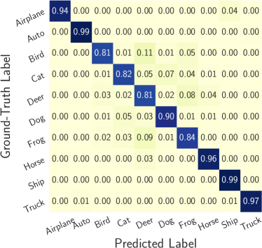
(a) Last Model (Train)

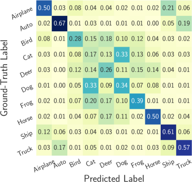
(b) Last Model (Test)

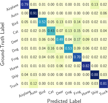
(c) Best Model (Train)

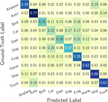
(d) Best Model (Test)

Figure 1: Heatmaps of predicted class distribution of training-time and testing-time generated adversarial examples with respect to models produced from the last epoch and the best epoch of adversarial training, where darker colors indicate larger probabilities.

To gain a deeper understanding of the phenomenon, we plot the heatmaps of the predicted label distribution for the adversarially-perturbed CIFAR-10 images in Figure 1, respectively generated by the model with the best robust generalization during adversarial training, denoted as Best Model, and the final model produced in the last epoch, denoted as Last Model. Here, the ground-truth label represents the underlying class of clean images and the predicted label is the class of adversarially-perturbed images generated by PGD-Attack predicted by the corresponding model. Figure 1 shows disparate characteristics between the label distributions of training- and testing-time adversarial examples with respect to the best and last models produced from adversarial training. Specifically, the testing-time predicted label distributions look much less certain than the training-time ones. Besides, in the training time, the distribution with respect to the Last Model mainly concentrates on the ground-truth class, whereas the Best Model with better robust generalization produces a more even distribution which is more similar to that of the corresponding testing samples. More experimental details about Figure 1 are provided in Appendix A.

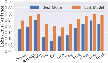
(a) Label-Level Variance

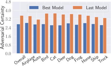
(b) Adversarial Certainty

Figure 2: Histograms of (a) label-level variances and (b) adversarial certainty of training-time adversarial examples generated by Last Model and Best Model across different CIFAR-10 classes.

Moreover, we measure the variance of the class probabilities of the predicted labels, denoted as label-level variance, with respect to the training-time adversarial examples for each ground-truth category in Figure 2(a). In particular, we observe that the Best Model with better robust generalization performance exhibits a lower label-level variance than that of the Last Model, which is consistent with the results illustrated in Figure 1. Even though the label-level variance best characterizes the predicted label distribution and reflects how certain the training-time generated adversarial examples are, such statistics are on a classwise distribution level, which is not easy to optimize. Therefore, we propose an alternative logit-level definition, termed as adversarial certainty, to capture the certainty of a model in classifying the adversarial examples generated by some attack method (e.g., PGD-Attack), where a lower value indicates lower model certainty in predicting adversarial examples:

Definition 3.1 (Adversarial Certainty).

Let $\mathcal{X}$ be the input space and $\mathcal{Y}$ be the label space. Suppose $\mu$ is the underlying distribution and $\mathcal{S}$ is a set of sampled examples. Let $\epsilon\geq 0$, $\Delta$ be the perturbation metric and $\mathcal{A}$ be some specific attack method for generating adversarial examples. For any neural network $M_{\theta}:\mathcal{X}\rightarrow\mathcal{Y}$, we define the adversarial certainty of $M_{\theta}$ with respect to $\mathcal{S}$ and $\mathcal{A}$ as:

$$\mathrm{AC}_{\epsilon}(M_{\theta};\mathcal{S},\mathcal{A})=\frac{1}{|\mathcal{S}|}\sum_{(\bm{x},y)\in\mathcal{S}}\mathrm{Var}\bigg{(}\widetilde{M}_{\theta}\big{[}\mathcal{A}(\bm{x};y,M_{\theta},\epsilon)\big{]}\bigg{)}.$$ (5)

Here, $\widetilde{M}_{\theta}:\mathcal{X}\rightarrow\mathbb{R}^{|\mathcal{Y}|}$ is the mapping from the input space to the logit layer of $M_{\theta}$ and $\mathrm{Var}(\bm{u})=\big{(}\sum_{k\in[K]}{(u_{k}-\overline{\bm{u}})}^{2}/K\big{)}^{1/2}$ for any $\bm{u}\in\mathbb{R}^{K}$, where $\overline{\bm{u}}$ denotes the average of all elements in $\bm{u}$.

Different from the label-level variance, adversarial certainty is an averaged sample-wise metric, which computes the variance of the logits returned by the model $M_{\theta}$ for each adversarially-perturbed example $\mathcal{A}(\bm{x};y,M_{\theta},\epsilon)$. Similar to Figure 2(a), we compute the adversarial certainty of the Best Model and the Last Model for each ground-truth category, which is further visualized in Figure 2(b). Since predicted labels are decided by the corresponding class with the highest predicted probabilities, the adversarial certainty depicts a similar pattern to the label-level variance as expected.

Our Perspective. Based on the empirical observations demonstrated in Figures 1 and 2, we further explain why model overconfidence is not beneficial for robust generalization, which is a potential cause for robust overfitting. Adversarial training aims to learn a model that can best classify the adversarial examples generated based on the model itself. Such an objective will encourage the model to keep improving its confidence in predicting the ground-truth with respect to the adversarially-perturbed training examples, which eventually leads to producing an overconfident model. However, this overconfidence property is detrimental to robust generalization, because the model cannot generate perturbed training inputs with low enough certainty, which is different from the typical generated adversarial examples during testing time. Consequently, the model will not be able to well predict the less certain test-time adversarial examples, thus resulting in a larger robust generalization gap between training and testing time. We hypothesize that such a large gap limits adversarially robust generalization. To the best of our knowledge, this perspective is new to the field of adversarial machine learning and is intuitively aligned with the classical machine learning theory that if the testing distribution deviates more from the training distribution (in our case, the prediction certainty of adversarial examples between training and testing), standard machine learners are expected to exhibit a decreased generalization performance (in our case, the robust generalization performance).

4 Decreasing Adversarial Certainty with Extragradient Steps

Motivated by the findings in Section 3, we propose a novel Extragradient-type method to explicitly Decrease Adversarial Certainty (EDAC), which searches for models with lower adversarial certainty by involving an extragradient step MLZFCP19 ; ZY20 in each training iteration to improve robust generalization. More specifically, EDAC aims to solve the following optimization problem to encourage models to generate less certain adversarial examples:

$$\min_{\theta\in\Theta}\>\frac{1}{|\mathcal{S}_{tr}|}\sum_{(\bm{x},y)\in\mathcal{S}_{tr}}\max_{\bm{x}^{\prime}\in\mathcal{B}_{\epsilon}(\bm{x})}L\big{(}M_{\theta^{\prime}},\bm{x}^{\prime},y\big{)},\text{where}\>\>\theta^{\prime}=\operatorname*{argmin}_{\theta^{\prime}\in\mathcal{C}(\theta)}\>\mathrm{AC}_{\epsilon}(M_{\theta^{\prime}};\mathcal{S}_{tr},\mathcal{A}),$$ (6)

where $\mathcal{S}_{tr}$ is the clean training dataset, $\mathcal{A}$ denotes a specific attack method (e.g., the PGD-Attack $\mathcal{A}_{\mathrm{pgd}}$), and $\mathcal{C}(\theta)$ represents the feasible search region for $\theta^{\prime}$. Here, $\theta^{\prime}$ can be understood as a function of $\theta$ which we aim to optimize in Equation 6. We remark that imposing the constraint of $\mathcal{C}(\theta)$ is necessary since adversarial certainty should be optimized towards that of testing examples to increase the training-testing similarity of predicted label distributions, whereas unconstrained optimization will cause $\theta^{\prime}$ deviating too much from the initial $\theta$, inducing a negative impact on robust generalization (see Figure 3(a) for more results and discussions regarding the design choice of the constraint set).

Directly solving the min-max-min problem specified in Equation 6 is challenging due to the non-convex nature of the optimization and the implicit definition of $\mathcal{C}(\theta)$, thus we resort to gradient-based methods for an approximate solver. To be more specific, we take the $(t+1)$-th iteration of adversarial training as an example to illustrate our design of EDAC. Given a set of clean training examples $\mathcal{S}_{tr}$, a specific attack method $\mathcal{A}$, and a classification model $M_{\theta}$, our EDAC method can be formulated as a two-step optimization for the $(t+1)$-th iteration:

$$\theta_{t+0.5} =\theta_{t}-\eta\cdot\nabla_{\theta}\mathrm{AC}_{\epsilon}(M_{\theta};\mathcal{S}_{tr},\mathcal{A})\Big{|}_{\theta=\theta_{t}},$$ (7)

$$\theta_{t+1} =\theta_{t+0.5}-\gamma\cdot\nabla_{\theta}L_{\mathrm{rob}}(M_{\theta};\mathcal{S}_{tr},\mathcal{A})\Big{|}_{\theta=\theta_{t+0.5}},$$

where $\eta>0$ and $\gamma>0$ represent the step sizes of the two optimization steps, $\mathrm{AC}_{\epsilon}(M_{\theta};\mathcal{S}_{tr},\mathcal{A})$ denotes the adversarial certainty of $M_{\theta}$ with respect to $\mathcal{S}_{tr}$ and $\mathcal{A}$ in Definition 3.1, and $L_{\mathrm{rob}}(M_{\theta};\mathcal{S}_{tr},\mathcal{A})$ can be roughly understood as a robust loss except the inner maximization is approximated using some attack method $\mathcal{A}$. The first step in Equation 7 optimizes the adversarial certainty, where it changes the model parameters $\theta_{t}$ in a direction that decreases the model’s adversarial certainty the most, whereas the second step in Equation 7 optimizes the model’s ability in distinguishing adversarial examples generated by the model itself as used in standard adversarial training.

As a result, the adversarial certainty of $M_{\theta_{t+0.5}}$ will be decreased after the first optimization step, i.e., $\mathrm{AC}_{\epsilon}(M_{\theta_{t+0.5}};\mathcal{S}_{tr},\mathcal{A})<\mathrm{AC}_{\epsilon}(M_{\theta_{t}};\mathcal{S}_{tr},\mathcal{A})$. According to the insights presented in Section 3, the model is expected to gain a better robust generalization ability after conducting the second optimization step on less certain adversarial examples generated based on $M_{\theta_{t+0.5}}$. Thus, as adversarial training proceeds, such decreased adversarial certainty and improved robust generalization ability will be iteratively learned to the final model, which mitigates the undesirable robust overfitting and improves model robustness. In each iteration, the extragradient step optimizes adversarial certainty to help find less certain adversarial examples corresponding to the current model status. This is why EDAC could work even if decreasing cross-entropy loss in the previous iteration and decreasing adversarial certainty in the current iteration are in different directions, i.e., $M_{\theta_{t+1}}$ will enjoy the newly optimized adversarial certainty, compared with $M_{\theta_{t}}$.

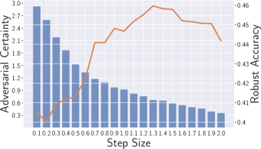
(a) Correlation Analysis

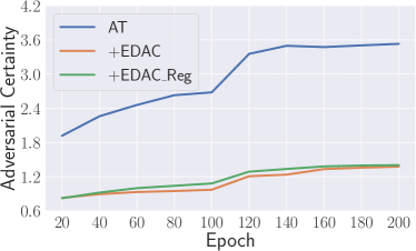
(b) Adversarial Certainty

Figure 3: (a) Correlation analysis between adversarial certainty and robust accuracy, where x-axis is the step size used in extra gradient, blue bars are training-time adversarial certainty, and the orange curve denotes robust test accuracy. (b) Training curves of adversarial certainty for different methods.

Correlation Analysis. Since our work aims to improve robust generalization by decreasing adversarial certainty, it is natural to ask the following question:

Does lower adversarial certainty imply better robust generalization?

Recall that in Equation 6, $\mathcal{C}(\theta)$ defines the feasible region for optimizing adversarial certainty. Therefore, the answer should intuitively be positive within this region, i.e., decreasing adversarial certainty will increase test robust accuracy. To better answer this question with empirical evidence, we conduct a correlation analysis between adversarial certainty and robust generalization. The results are illustrated in Figure 3(a). Specifically, we use an AT-trained model as the starting point, from which the heatmaps (Figure 1) are derived. Then, we separately update one more epoch on the model by EDAC using different step sizes (from 0.1 to 2.0) in extragradient steps to decrease adversarial certainty. Afterward, we measure the training-time adversarial certainty (i.e., the blue bars) and robust test accuracy (i.e., the orange curve) of the result models. As expected, adversarial certainty keeps decreasing with the increase in step size. Meanwhile, the model robustness first keeps improving, but it decreases when the step size is larger than 1.3. These results indicate that when the step size is appropriately selected, the optimized model parameters are still within the feasible search region, wherein lower training-time adversarial certainty corresponds to higher robustness. However, when the model is out of the feasible search region, decreasing adversarial certainty will not help improve robust generalization anymore.

Why Extragradient Steps? Our algorithmic design of utilizing extragradient steps is inspired by the existing literature on min-max optimization DP18 ; DDJ21 ; HMC21 ; PLPFC22 . In particular, these related works illustrate that standard first-order methods, such as stochastic gradient descent/ascent (SGDA), can converge to recurrent orbits that do not contain any critical point of the underlying min-max problem, regardless of the basic convex-concave regime or general non-convex/non-concave problems. Extragradient-type methods have been studied as a first-order alternative to SGDA that can avoid such failure modes and have proven to be a principled way to find local solutions (e.g., a stationary point) to the underlying min-max problems under various settings. This sheds light on the potential of using extragradient steps to solve min-max problems more effectively. Nevertheless, our proposed method that optimizes for adversarial robustness is slightly different from the standard extragradient method typically studied in the optimization literature, because the extra gradient is computed with respect to adversarial certainty instead of cross-entropy loss. Still, it shares a similar insight of escaping the failure mode of the standard first-order min-max solver with the help of extragradient steps. As will be demonstrated in Section 5, the introduced extragradient step for optimizing adversarial certainty is essential to obtain a stable and improved robustness performance across various benchmarks and different settings compared with other regularization-based optimization schemes.

Application Scope. Our method can be summarized as a two-step iterative optimization framework: $\theta_{t}{\longrightarrow}\theta_{t+0.5}{\longrightarrow}\theta_{t+1}.$ We remark that this framework provides a generic way to explicitly optimize a specified property (e.g., adversarial certainty) in the first step, and then to take advantage of the newly generated training samples with a better property to find a more robust model in the second step. Intuitively, this framework is generally applicable to any adversarial defense that requires training-time adversarial examples generated based on the to-be-updated model, because the optimization of adversarial robustness relies on the generated adversarial examples, i.e., training samples with updated properties would benefit model robustness. In Section 5, we will examine the compatibility of our EDAC method with several PGD-based methods, including adversarial training and its variants.

5 Experiments

In this section, we evaluate the effectiveness of our EDAC method in improving robust generalization with respect to different model architecture PreActResNet-18 (PRN18) and WideResNet-34 (WRN34) under the threat model of $\ell_{\infty}$ trained by several benchmark adversarial defenses, i.e., AT pgd , TRADES trades and MART mart on CIFAR-10 in Section 5.1. Besides, to examine the generalizability to other settings, we provide results of EDAC on more benchmark datasets, including CIFAR-10, CIFAR-100 and SVHN, and $\ell_{2}$ norm-bounded perturbations. Then, in Section 5.2, we evaluate the compatibility of EDAC with AWP awp and Consistency consistency .

Experimental Settings. For the $\ell_{\infty}$ threat model, we set $\epsilon=8/255$, and train the model for 200 epochs using SGD with the momentum of 0.9. Besides, the initial learning rate is 0.1, and is divided by 10 at the $100^{th}$ epoch and at the $150^{th}$ epoch. And the adversarial attack used in training is PGD-10 with a step size of $1/255$ for SVHN, and $2/255$ for CIFAR-10 and CIFAR-100, while we utilize the commonly-used attack benchmarks of PGD-20 pgd , PGD-100 pgd , $\text{CW}_{\infty}$ CW17 and AutoAttack autoattack in testing. Meanwhile, for the $\ell_{2}$ threat model, we set $\epsilon=128/255$ with a step size of $15/255$ for all datasets. In addition, we also measure the Clean performance to investigate the influence on clean images. Regarding other hyperparameters, we follow the settings described in their original papers. In all cases, we evaluate the performance of the last (best) model in terms of testing-time robust accuracy.

5.1 Main Results

Table 1: Testing-time adversarial robustness (%) with/without EDAC on CIFAR-10 under $\ell_{\infty}$ threat model across different model architectures and adversarial training methods.

Architecture	Method	Clean	PGD-20	PGD-100	$\text{CW}_{\infty}$	AutoAttack
PRN18	AT	82.88 (82.68)	41.51 (49.23)	40.96 (48.92)	41.61 (48.07)	39.66 (45.71)
	+ EDAC	84.64 (83.55)	45.55 (52.20)	44.94 (51.87)	44.55 (50.05)	42.78 (48.20)
	TRADES	82.10 (81.33)	47.44 (51.65)	46.95 (51.42)	46.64 (49.18)	44.99 (48.06)
	+ EDAC	83.18 (82.80)	49.32 (52.90)	48.81 (52.67)	48.30 (50.11)	46.40 (48.96)
	MART	80.85 (78.27)	50.23 (52.28)	49.71 (52.13)	46.88 (47.83)	44.68 (46.01)
	+ EDAC	81.12 (79.37)	52.38 (53.25)	52.04 (53.14)	48.97 (49.25)	47.24 (47.69)
WRN34	AT	86.47 (85.86)	47.25 (55.31)	46.73 (55.00)	47.85 (54.04)	45.84 (51.94)
	+ EDAC	86.48 (85.10)	52.02 (57.93)	51.69 (57.68)	51.51 (54.98)	49.75 (53.33)
	TRADES	86.01 (84.74)	49.66 (53.72)	48.44 (53.60)	48.56 (52.35)	46.53 (51.31)
	+ EDAC	86.75 (85.18)	53.70 (55.86)	53.09 (55.59)	52.73 (53.72)	50.50 (52.42)
	MART	83.11 (81.31)	48.93 (53.87)	48.31 (53.68)	46.32 (49.65)	44.89 (48.00)
	+ EDAC	84.69 (83.23)	52.00 (55.57)	51.32 (55.22)	49.50 (51.43)	47.65 (49.92)

Results on CIFAR-10. We evaluate the robust generalization of our proposed EDAC on CIFAR-10, a commonly-used image benchmark. The results are depicted in Table 1. We can see that, EDAC significantly enhances testing-time adversarial robustness across different adversarial attacks. These results show the effectiveness of EDAC, indicating the significance of less certain adversarial examples for robust generalization. Besides, we investigate the influence of EDAC on robust overfitting which is an attention-worthy phenomenon. Specifically, Figure 4(a) evaluates the gap of testing-time adversarial robustness between the best and the last models. We can observe that EDAC consistently mitigates robust overfitting across different settings. These results indicate that decreasing adversarial certainty could mitigate the degradation of robust generalization induced by robust overfitting.

Moreover, we find that WRN34 suffers from more severe robust overfitting in adversarial training, however, could benefit more mitigation by using our EDAC method. This suggests that WRN34 is superior to PRN18 in terms of robust generalization with the help of EDAC. Besides adversarial robustness, the clean accuracy for testing images is also worth attention since they measure the standard generalization ability of the model. As expected, EDAC consistently improves the clean test accuracy in all cases as shown in the Clean column of Table 1. This promotion shows that EDAC also could help models gain better robustness against unseen clean images even by learning from adversarial examples, which also benefits from the improvement of generalization.

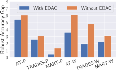
(a) Robust Overfitting

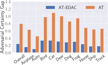
(b) Adversarial Certainty Gap

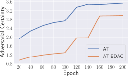
(c) AT

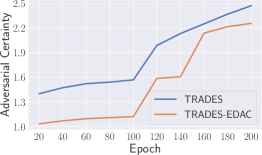
(d) TRADES

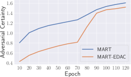
(e) MART

Figure 4: The visualized results evaluating robust overtfitting and adversarial certainty, where “-P” and “-W” in the x-axis of Figure 4(a) represent PRN18 and WRN34 respectively.

EDAC Improves Adversarial Certainty. Since EDAC has empirically shown effective to improve robust generalization, in this part, we want to demonstrate this is because EDAC could decrease adversarial certainty. To this end, we train a sequence of models by AT and TRADES for 200 epochs, and by MART for 120 epochs, respectively. And for every 20 epochs in this sequence, we update the same intermediate model by one further epoch using the original adversarial defenses with and without the help of EDAC, respectively. Then, we measure the adversarial certainty of all further-updated models following Equation 5. In Figure 4(c), we compare AT with AT-EDAC and observe that – consistent with our findings in Section 3 and design purpose explained in Section 4 – EDAC could indeed help models generate less certain adversarial examples, which would bring better robust generalization. The cases of TRADES and MART are measured in Figures 4(d) and 4(e) respectively, which show similar trends. Moreover, we measure the adversarial certainty gap between the best model and the last model on AT and AT-EDAC in Figure 4(b). We find that the adversarial certainty gap of AT-EDAC is significantly smaller, which is aligned with the closer adversarial robustness of the best model and the last model. This result explains why EDAC could mitigate robust overfitting by decreasing adversarial certainty in extragradient steps.

Table 2: Testing-time adversarial robustness (%) of AT with/without EDAC/EDAC_Reg under $\ell_{\infty}$ threat model across different model architectures and benchmark datasets.

Dataset	Architecture	Method	Clean	PGD-20	PGD-100	$\text{CW}_{\infty}$	AutoAttack
SVHN	PRN18	AT	89.63 (88.64)	42.25 (51.00)	41.37 (50.30)	42.84 (48.19)	39.52 (46.02)
		+ EDAC	90.58 (89.63)	45.86 (54.42)	43.92 (53.78)	43.75 (50.15)	40.68 (48.23)
		+ EDAC_Reg	90.65 (90.21)	45.39 (53.06)	43.77 (52.28)	43.66 (49.64)	41.10 (47.39)
	WRN34	AT	91.51 (89.72)	46.81 (53.43)	44.94 (52.77)	45.76 (50.43)	41.71 (49.50)
		+ EDAC	91.26 (91.83)	60.42 (67.95)	56.71 (64.85)	56.98 (65.09)	42.33 (50.42)
		+ EDAC_Reg	91.76 (92.13)	62.19 (65.96)	59.54 (63.68)	60.05 (63.87)	42.46 (49.95)
CIFAR-10	PRN18	AT	82.88 (82.68)	41.51 (49.23)	40.96 (48.92)	41.61 (48.07)	39.66 (45.71)
		+ EDAC	84.64 (83.55)	45.55 (52.20)	44.94 (51.87)	44.55 (50.05)	42.78 (48.20)
		+ EDAC_Reg	83.78 (83.54)	45.39 (50.86)	44.87 (50.49)	44.18 (48.96)	42.41 (47.02)
	WRN34	AT	86.47 (85.86)	47.25 (55.31)	46.73 (55.00)	47.85 (54.04)	45.84 (51.94)
		+ EDAC	86.48 (85.10)	52.02 (57.93)	51.69 (57.68)	51.51 (54.98)	49.75 (53.33)
		+ EDAC_Reg	85.69 (76.89)	48.81 (48.91)	47.54 (48.86)	47.55 (45.98)	44.24 (44.99)
CIFAR-100	PRN18	AT	54.58 (53.64)	20.29 (27.80)	20.00 (27.66)	20.18 (25.40)	18.52 (23.45)
		+ EDAC	54.85 (55.01)	22.46 (27.73)	22.19 (27.48)	21.11 (25.37)	19.09 (23.95)
		+ EDAC_Reg	54.67 (53.11)	21.78 (28.86)	21.50 (28.70)	20.56 (26.00)	19.29 (23.40)
	WRN34	AT	57.23 (54.45)	25.64 (30.30)	25.38 (29.97)	24.09 (27.57)	22.76 (25.46)
		+ EDAC	58.15 (58.04)	26.08 (31.55)	25.89 (31.43)	24.77 (29.19)	23.66 (27.08)
		+ EDAC_Reg	57.57 (58.34)	24.46 (30.97)	24.13 (30.89)	24.04 (28.92)	22.68 (26.71)

Alternative Regularization Method. As we only conceptually illustrate involving extragradient steps for EDAC in Section 4, this section will empirically demonstrate the necessity of this decision by comparing EDAC with decreasing adversarial certainty without extragradient steps. Specifically, we construct a regularization term to decrease the adversarial certainty, and add it to robust loss. Then, similar to adversarial training, in each iteration, we only conduct a single step of optimization according to the regularized robust loss, which is termed as EDAC_Reg. The full results on SVHN, CIFAR-10 and CIFAR-100 datasets with both PRN18 and WRN34 models are shown in Table 2.

We can see that EDAC_Reg could improve the robust generalization of AT due to the regularization to decrease adversarial certainty, but EDAC brings better and more stable improvements, which indicates the advantage of involving extragradient steps. In some cases, EDAC_Reg is even harmful to robust generalization, e.g., when a WideResNet-34-10 model is trained on CIFAR-10. These results comply with our discussion in Section 4 that existing literature on min-max optimization shows the potential of using extragradient-type methods to avoid limit cycles with respect to standard gradient descent/ascent approaches. In addition, we measure the adversarial certainty of a sequence of models trained by AT, EDAC and EDAC_Reg, respectively, in Figure 3(b). We could observe that EDAC gains the lowest adversarial certainty (even only with a slight gap over EDAC_Reg), indicating that higher robust generalization corresponds to lower adversarial certainty.

Other Benchmark Datasets. We extend the robustness evaluation of EDAC to more benchmark datasets, including SVHN svhn , CIFAR-10 CIFAR and CIFAR-100 CIFAR . Table 2 shows that EDAC consistently improves robust generalization across different datasets. In particular, EDAC could increase the adversarial robustness on SVHN by 14.52% for the WRN34 best model of AT against PGD-20. These improvements further confirm the effectiveness and generalizability of EDAC.

Table 3: Testing-time adversarial robustness (%) of AT with/without EDAC on PreActResNet-18 under $\ell_{2}$ threat model against PGD-20 across different benchmark datasets.

Method	SVHN		CIFAR-10		CIFAR-100
	Best	Last	Best	Last	Best	Last
AT (Madry et al. 2018)	66.45	63.20	66.02	65.18	39.23	35.68
+ EDAC	69.11	67.44	69.10	67.37	40.75	36.32

$\ell_{2}$ Norm-Bounded Perturbation. In the above evaluation, we focus on the $\ell_{\infty}$ norm-bounded perturbations. Meanwhile, the $\ell_{2}$ norm is also a prevalent perturbation setting in adversarial training. Thus, in Table 3, we evaluate our method under the $\ell_{2}$ threat model. Similarly, EDAC depicts consistent improvements in adversarial robustness on best and last epochs and different benchmark datasets, which shows the efficacy of EDAC against adversarial attacks with $\ell_{2}$ perturbations.

5.2 Extension to Other Adversarial Training Methods

Table 4: Testing-time adversarial robustness (%) of AWP and Consistency with/without EDAC on CIFAR-10 and PRN18 under $\ell_{\infty}$ threat model.

Method	Clean	PGD-20	PGD-100	$\text{CW}_{\infty}$	AutoAttack
AT-AWP	83.76 (82.37)	52.99 (54.04)	52.71 (53.89)	51.07 (51.22)	48.75 (49.33)
+ EDAC	84.07 (82.67)	54.55 (55.17)	54.30 (55.00)	51.76 (52.03)	49.80 (49.96)
TRADES-AWP	81.46 (81.28)	52.71 (53.69)	52.54 (53.55)	50.37 (50.61)	49.54 (49.92)
+ EDAC	82.69 (82.85)	54.06 (54.68)	53.80 (54.49)	51.44 (51.53)	50.51 (50.63)
MART-AWP	78.13 (77.27)	53.26 (53.62)	53.06 (52.58)	49.05 (48.39)	46.53 (47.01)
+ EDAC	80.03 (78.65)	54.79 (55.16)	54.67 (54.93)	49.58 (49.14)	47.47 (47.73)
AT-Consistency	85.28 (84.66)	55.43 (56.72)	55.16 (56.46)	50.81 (51.13)	48.08 (48.48)
+ EDAC	85.36 (85.17)	56.65 (57.19)	56.31 (56.90)	51.29 (51.72)	49.00 (49.46)
TRADES-Consistency	83.68 (83.51)	53.00 (53.06)	52.78 (52.79)	48.85 (48.89)	47.75 (47.77)
+ EDAC	84.78 (84.73)	53.73 (53.96)	53.48 (53.72)	49.37 (49.41)	48.15 (48.19)
MART-Consistency	78.21 (78.11)	56.33 (56.85)	56.31 (56.81)	47.33 (47.47)	45.53 (45.73)
+ EDAC	81.91 (81.35)	58.59 (58.76)	58.29 (58.56)	50.08 (50.21)	48.28 (48.59)

Previous sections show the efficacy of EDAC on adversarial training and its variants. We note that some recent works also focus on understanding robust generalization and developing methods to improve adversarial training towards more robust models, including Adversarial Weight Perturbation awp – AWP for short – and Consistency Reguarlaization consistency – Consistency for short. However, since these methods focus on different insights to improve robust generalization, whether our proposed EDAC framework is compatible with them remains elusive. In this section, we study the generalizability of our EDAC to AWP and Consistency regularization, which is depicted in Table 4.

Adversarial Weight Perturbation. AWP discovered that the flatness of the weight loss landscape is an important factor related to robust generalization, while EDAC seeks less certain training-time adversarial examples. AWP shares some similarities with our work, where both EDAC and AWP find new model status by gradient-based method before optimizing model robustness, i.e., in the $(t+1)$-th iteration, model parameters $\theta_{t+1}$ is derived from the optimization on $\theta_{t+0.5}$, instead of directly from $\theta_{t}$. However, there is a main difference between AWP and our work: In our work, $\theta_{t+0.5}\longrightarrow\theta_{t+1}$ is optimized on the adversarial examples generated by $\theta_{t+0.5}$, which takes advantage of the optimized adversarial certainty of $\theta_{t+0.5}$, while AWP uses the adversarial examples generated by $\theta_{t}$ to derive $\theta_{t+1}$. Consequently, EDAC and AWP aim at different directions to help models. In that case, we attempt to cooperate EDAC with AWP by adding another extragradient step before weight perturbation to optimize the certainty of adversarial examples, and use the updated intermediate model to generate new adversarial examples for the following AWP optimization. As shown in Table 4, EDAC could compatibly work with AWP and gain further improvements in robust generalization.

Consistency Regularization. The method of Consistency regularizes the adversarial consistency based on various data augmentations consistency . In that case, we first use extragradient steps to update the adversarial certainty on augmented samples, and then follow the Consistency optimization. From Table 4, we can see that EDAC could cooperatively improve the robust generalization of Consistency, which shows the feasibility of EDAC in the augmentation-based domain.

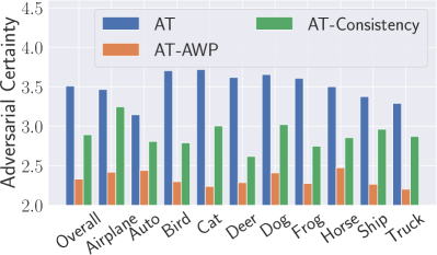
(a) Last Model

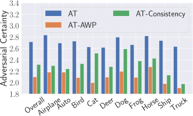
(b) Best Model

Figure 5: The visualized results on CIFAR-10 with respect to PRN18 for comparing adversarial certainty of AT, AT-AWP and AT-Consistency based on (a) last model, and (b) best model.

In general, the improvement of EDAC on AWP and Consistency is not as significant as previous ones. We hypothesize this is because AWP and Consistency could implicitly decrease adversarial certainty when helping models toward their specified directions. Thus, when EDAC conducts the explicit optimization of adversarial certainty, it can only achieve slight improvements that are derived from less certain training samples generated in extragradient steps. To this end, we measure the adversarial certainty of AWP and Consistency on the last and the best models of AT in Figure 5. We could see that both methods of AT-AWP and AT-Consistency, which achieve better robust generalization performance than AT, also implicitly decrease the adversarial certainty. This suggests that different insights for helping model robustness would be compatible with each other to some extent, but how to coordinate them for a better unified improvement is worth exploring in the future.

6 Conclusion

We revisited the robust overfitting phenomenon of adversarial training and discovered that overfitting to training data might result from the training-time adversarial examples generated by overconfident models. Specifically, we observed that models with better robust generalization performance correspond to significantly more even predicted label distributions of training-time adversarial examples. Built upon a new notion of adversarial certainty, we proposed to involve an extragradient step to generate less certain examples by decreasing adversarial certainty, which can be combined with various attack methods for generating adversarial examples. Extensive experiments substantiated the effectiveness of our method in mitigating robust overfitting and learning more robust models.

Availability

Our implementation is available as open-source code at https://github.com/TrustMLRG/EDAC.

Appendix

Appendix A Details of Section 3

In this section, we explain the experimental details for producing the heatmaps and the histograms illustrated in Section 3. Given a model $M_{\theta}$ (e.g., Best Model and Last Model) and a set of examples $\mathcal{S}$ sampled from the underlying distribution $\mu$ (e.g., CIFAR-10 training and testing datasets), adversarial examples are generated by the PGD-Attack within the perturbation ball $\mathcal{B}_{\epsilon}(\bm{x})$ centered at $\bm{x}$ with radius $\epsilon=8/255$ under the $\ell_{\infty}$ threat model, which follows the settings of generating training samples in Section 5, e.g., the PGD-Attack is iteratively conducted by $10$ steps with the step size of $2/255$. We record the predicted labels of the generated adversarial examples with respect to each model, and then plot the classwise label distributions as heatmaps in Figure 1.

In general, let $\mathrm{HM}$ be the $m\times m$ matrix representing the heatmap, where $\mathcal{Y}=\{1,2,\ldots,m\}$ denotes the label space. For any $j,k\in\mathcal{Y}$, the $(j,k)$-th entry of $\mathrm{HM}$ with respect to $M_{\theta}$ and $\mathcal{S}$ is defined as:

$$\mathrm{HM}_{j,k}=\frac{\bigg{|}\big{\{}(\bm{x},y)\in\mathcal{S}:y=j\>\text{ and }\>M_{\theta}\big{(}\mathcal{A}_{\mathrm{pgd}}(\bm{x};y,M_{\theta},\epsilon)\big{)}=k\big{\}}\bigg{|}}{\bigg{|}\big{\{}(\bm{x},y)\in\mathcal{S}:y=j\big{\}}\bigg{|}},$$ (8)

where $\mathcal{A}_{\mathrm{pgd}}$ is the PGD-Attack defined by the update rule 4. More specifically, for any $(\bm{x},y)\in\mathcal{S}$, we construct the corresponding adversarial example by the PGD-Attack, i.e., $\bm{x}^{\prime}=\mathcal{A}_{\mathrm{pgd}}(\bm{x};y,M_{\theta},\epsilon)\big{)}$. Then, we measure the predicted label $\hat{y}=M_{\theta}(\bm{x}^{\prime})$. In that case, for the given training data, we could construct $(\textit{ground-truth},\textit{predicted})$ label pairs, simply denoted by $\{(y,\hat{y})\}$. Afterward, we first cluster $\{(y,\hat{y})\}$ separately by the ground-truth label, e.g., the subset of ground-truth label $j$ includes all pairs such that $y=j$ (denoted by $\{(y,\hat{y})\}_{j}$), which corresponds to the rows of heatmaps. Further, for each subset, we group it into sub-subsets separately by the predicted labels, e.g., $\{(y,\hat{y})\}_{j,k}$ contains all pairs in $\{(y,\hat{y})\}_{j}$ such that $\hat{y}=k$. Consequently, the number of adversarial examples of the ground truth label $j$ is calculated as:

$$|\{(y,\hat{y})\}_{j}|=\bigg{|}\big{\{}(\bm{x},y)\in\mathcal{S}:y=j\big{\}}\bigg{|}.$$

Meanwhile, the number of adversarial examples of ground truth label $j$ but predicted as label $k$ is measured as:

$$|\{(y,\hat{y})\}_{j,k}|=\bigg{|}\big{\{}(\bm{x},y)\in\mathcal{S}:y=j\>\text{ and }\>M_{\theta}\big{(}\mathcal{A}_{\mathrm{pgd}}(\bm{x};y,M_{\theta},\epsilon)\big{)}=k\big{\}}\bigg{|},$$

where $\hat{y}=M_{\theta}\big{(}\mathcal{A}_{\mathrm{pgd}}(\bm{x};y,M_{\theta},\epsilon)\big{)}$. Finally, we compute the $(j,k)$-th entry of the heatmap $\mathrm{HM}_{j,k}$ as the ratio of $|\{(y,\hat{y})\}_{j,k}|$ to $|\{(y,\hat{y})\}_{j}|$, i.e., Equation 8.

Moreover, following the same settings, we plot the corresponding label-level variance and adversarial certainty in Figure 2. Specifically, we first measure the label-level variance of the training-time adversarial examples of the last model (Figure 1(a)) and the best model (Figure 1(c)) conditioned on the ground-truth label, as shown in Figure 2(a). Taking the ground-truth label $j$ as an example, the label-level variance can be formulated as:

$$\mathrm{Var}_{j}^{\mathrm{(label)}}=\sqrt{\frac{1}{|\mathcal{Y}|}\sum_{k\in\mathcal{Y}}(\mathrm{HM}_{j,k}-\overline{\mathrm{HM}}_{j})^{2}},$$

where $\overline{\mathrm{HM}}_{j}$ averages all $\mathrm{HM}_{j,k}$ with different $k$, and $\mathcal{Y}=\{1,2,...,m\}$ is the label space.

In addition, according to Equation 5 defined in Section 3, we measure the adversarial certainty of the last and the best models, as illustrated in Figure 2(b), with respect to the predicted logits of all the adversarial examples conditioned on the ground-truth label.

References

- [1] Jean-Baptiste Alayrac, Jonathan Uesato, Po-Sen Huang, Alhussein Fawzi, Robert Stanforth, and Pushmeet Kohli. Are labels required for improving adversarial robustness? In Annual Conference on Neural Information Processing Systems (NeurIPS), pages 12192–12202. NeurIPS, 2019.
- [2] Maksym Andriushchenko and Nicolas Flammarion. Understanding and improving fast adversarial training. In Annual Conference on Neural Information Processing Systems (NeurIPS). NeurIPS, 2020.
- [3] Nicholas Carlini and David Wagner. Towards Evaluating the Robustness of Neural Networks. In IEEE Symposium on Security and Privacy (S&P), pages 39–57. IEEE, 2017.
- [4] Yair Carmon, Aditi Raghunathan, Ludwig Schmidt, John C. Duchi, and Percy Liang. Unlabeled data improves adversarial robustness. In Annual Conference on Neural Information Processing Systems (NeurIPS), pages 11190–11201. NeurIPS, 2019.
- [5] Chenyi Chen, Ari Seff, Alain Kornhauser, and Jianxiong Xiao. Deepdriving: Learning affordance for direct perception in autonomous driving. In IEEE International Conference on Computer Vision (ICCV), pages 2722–2730. IEEE, 2015.
- [6] Tianlong Chen, Zhenyu Zhang, Sijia Liu, Shiyu Chang, and Zhangyang Wang. Robust overfitting may be mitigated by properly learned smoothening. In International Conference on Learning Representations, 2021.
- [7] Jeremy M. Cohen, Elan Rosenfeld, and J. Zico Kolter. Certified Adversarial Robustness via Randomized Smoothing. In International Conference on Machine Learning (ICML), pages 1310–1320. PMLR, 2019.
- [8] Paul Covington, Jay Adams, and Emre Sargin. Deep neural networks for youtube recommendations. In ACM Conference on Recommender Systems (RecSys), pages 191–198. ACM, 2016.
- [9] Francesco Croce, Maksym Andriushchenko, Vikash Sehwag, Edoardo Debenedetti, Nicolas Flammarion, Mung Chiang, Prateek Mittal, and Matthias Hein. Robustbench: a standardized adversarial robustness benchmark. arXiv preprint arXiv:2010.09670, 2020.
- [10] Francesco Croce and Matthias Hein. Reliable evaluation of adversarial robustness with an ensemble of diverse parameter-free attacks. In International Conference on Machine Learning (ICML), pages 2206–2216. PMLR, 2020.
- [11] Constantinos Daskalakis and Ioannis Panageas. The limit points of (optimistic) gradient descent in min-max optimization. In Annual Conference on Neural Information Processing Systems (NeurIPS), pages 9256–9266. NeurIPS, 2018.
- [12] Jacob Devlin, Ming-Wei Chang, Kenton Lee, and Kristina Toutanova. BERT: Pre-training of Deep Bidirectional Transformers for Language Understanding. In Conference of the North American Chapter of the Association for Computational Linguistics: Human Language Technologies (NAACL-HLT), pages 4171–4186. ACL, 2019.
- [13] Jelena Diakonikolas, Constantinos Daskalakis, and Michael I. Jordan. Efficient methods for structured nonconvex-nonconcave min-max optimization. In International Conference on Artificial Intelligence and Statistics AISTATS, pages 2746–2754. PMLR, 2021.
- [14] Samuel G Finlayson, John D Bowers, Joichi Ito, Jonathan L Zittrain, Andrew L Beam, and Isaac S Kohane. Adversarial attacks on medical machine learning. Science, pages 1287–1289, 2019.
- [15] Ruiqi Gao, Tianle Cai, Haochuan Li, Cho-Jui Hsieh, Liwei Wang, and Jason D Lee. Convergence of adversarial training in overparametrized neural networks. Advances in Neural Information Processing Systems, 32, 2019.
- [16] Ian Goodfellow, Jonathon Shlens, and Christian Szegedy. Explaining and Harnessing Adversarial Examples. In International Conference on Learning Representations (ICLR), 2015.
- [17] Kaiming He, Xiangyu Zhang, Shaoqing Ren, and Jian Sun. Deep residual learning for image recognition. In IEEE Conference on Computer Vision and Pattern Recognition (CVPR), pages 770–778. IEEE, 2016.
- [18] Ya-Ping Hsieh, Panayotis Mertikopoulos, and Volkan Cevher. The limits of min-max optimization algorithms: Convergence to spurious non-critical sets. In International Conference on Machine Learning ICML, pages 4337–4348. PMLR, 2021.
- [19] Joong-won Hwang, Youngwan Lee, Sungchan Oh, and Yuseok Bae. Adversarial training with stochastic weight average. In IEEE International Conference on Image Processing (ICIP), pages 814–818. IEEE, 2021.
- [20] Gaojie Jin, Xinping Yi, Wei Huang, Sven Schewe, and Xiaowei Huang. Enhancing adversarial training with second-order statistics of weights. In IEEE Conference on Computer Vision and Pattern Recognition (CVPR), pages 15252–15262. IEEE, 2022.
- [21] Can Kanbak, Seyed-Mohsen Moosavi-Dezfooli, and Pascal Frossard. Geometric robustness of deep networks: analysis and improvement. In Proceedings of the IEEE Conference on Computer Vision and Pattern Recognition, pages 4441–4449, 2018.
- [22] Stepan Komkov and Aleksandr Petiushko. Advhat: Real-world adversarial attack on arcface face id system. In IEEE International Conference on Pattern Recognition (ICPR), pages 819–826. IEEE, 2021.
- [23] Alex Krizhevsky and Geoffrey Hinton. Learning multiple layers of features from tiny images. 2009.
- [24] Xingjun Ma, Bo Li, Yisen Wang, Sarah M. Erfani, Sudanthi N. R. Wijewickrema, Grant Schoenebeck, Dawn Song, Michael E. Houle, and James Bailey. Characterizing adversarial subspaces using local intrinsic dimensionality. In International Conference on Learning Representations (ICLR), 2018.
- [25] Xingjun Ma, Yuhao Niu, Lin Gu, Yisen Wang, Yitian Zhao, James Bailey, and Feng Lu. Understanding adversarial attacks on deep learning based medical image analysis systems. Pattern Recognition, 110:107332, 2021.
- [26] Aleksander Madry, Aleksandar Makelov, Ludwig Schmidt, Dimitris Tsipras, and Adrian Vladu. Towards Deep Learning Models Resistant to Adversarial Attacks. In International Conference on Learning Representations (ICLR), 2018.
- [27] Panayotis Mertikopoulos, Bruno Lecouat, Houssam Zenati, Chuan-Sheng Foo, Vijay Chandrasekhar, and Georgios Piliouras. Optimistic mirror descent in saddle-point problems: Going the extra (gradient) mile. In International Conference on Learning Representations (ICLR), 2019.
- [28] Yuval Netzer, Tao Wang, Adam Coates, Alessandro Bissacco, Bo Wu, and Andrew Y Ng. Reading digits in natural images with unsupervised feature learning. 2011.
- [29] Nicolas Papernot, Patrick D. McDaniel, Xi Wu, Somesh Jha, and Ananthram Swami. Distillation as a Defense to Adversarial Perturbations Against Deep Neural Networks. In IEEE Symposium on Security and Privacy (S&P), pages 582–597. IEEE, 2016.
- [30] Thomas Pethick, Puya Latafat, Panos Patrinos, Olivier Fercoq, and Volkan Cevher. Escaping limit cycles: Global convergence for constrained nonconvex-nonconcave minimax problems. In International Conference on Learning Representations ICLR, 2022.
- [31] Sylvestre-Alvise Rebuffi, Sven Gowal, Dan A Calian, Florian Stimberg, Olivia Wiles, and Timothy Mann. Fixing data augmentation to improve adversarial robustness. arXiv preprint arXiv:2103.01946, 2021.
- [32] Leslie Rice, Eric Wong, and J. Zico Kolter. Overfitting in adversarially robust deep learning. In International Conference on Machine Learning (ICML), pages 8093–8104. PMLR, 2020.
- [33] Amrith Setlur, Benjamin Eysenbach, Virginia Smith, and Sergey Levine. Adversarial unlearning: Reducing confidence along adversarial directions. In Annual Conference on Neural Information Processing Systems (NeurIPS). NeurIPS, 2022.
- [34] Ali Shafahi, Mahyar Najibi, Amin Ghiasi, Zheng Xu, John P. Dickerson, Christoph Studer, Larry S. Davis, Gavin Taylor, and Tom Goldstein. Adversarial training for free! In Annual Conference on Neural Information Processing Systems (NeurIPS), pages 3353–3364. NeurIPS, 2019.
- [35] Mahmood Sharif, Lujo Bauer, and Michael K Reiter. On the suitability of lp-norms for creating and preventing adversarial examples. In Proceedings of the IEEE Conference on Computer Vision and Pattern Recognition Workshops, pages 1605–1613, 2018.
- [36] David Stutz, Matthias Hein, and Bernt Schiele. Confidence-calibrated adversarial training: Generalizing to unseen attacks. In International Conference on Machine Learning (ICML), volume 119, pages 9155–9166. PMLR, 2020.
- [37] David Stutz, Matthias Hein, and Bernt Schiele. Relating adversarially robust generalization to flat minima. In IEEE International Conference on Computer Vision (ICCV), pages 7787–7797. IEEE, 2021.
- [38] Christian Szegedy, Wojciech Zaremba, Ilya Sutskever, Joan Bruna, Dumitru Erhan, Ian Goodfellow, and Rob Fergus. Intriguing Properties of Neural Networks. In International Conference on Learning Representations (ICLR), 2014.
- [39] Jihoon Tack, Sihyun Yu, Jongheon Jeong, Minseon Kim, Sung Ju Hwang, and Jinwoo Shin. Consistency regularization for adversarial robustness. In AAAI Conference on Artificial Intelligence (AAAI), pages 8414–8422. AAAI, 2022.
- [40] Florian Tramèr, Alexey Kurakin, Nicolas Papernot, Ian Goodfellow, Dan Boneh, and Patrick McDaniel. Ensemble Adversarial Training: Attacks and Defenses. In International Conference on Learning Representations (ICLR), 2017.
- [41] Zhuozhuo Tu, Jingwei Zhang, and Dacheng Tao. Theoretical analysis of adversarial learning: A minimax approach. Advances in Neural Information Processing Systems, 32, 2019.
- [42] Yisen Wang, Difan Zou, Jinfeng Yi, James Bailey, Xingjun Ma, and Quanquan Gu. Improving Adversarial Robustness Requires Revisiting Misclassified Examples. In International Conference on Learning Representations (ICLR), 2020.
- [43] Zekai Wang, Tianyu Pang, Chao Du, Min Lin, Weiwei Liu, and Shuicheng Yan. Better diffusion models further improve adversarial training. arXiv preprint arXiv:2302.04638, 2023.
- [44] Eric Wong, Leslie Rice, and J. Zico Kolter. Fast is better than free: Revisiting adversarial training. In International Conference on Learning Representations (ICLR), 2020.
- [45] Dongxian Wu, Shu-Tao Xia, and Yisen Wang. Adversarial weight perturbation helps robust generalization. In Annual Conference on Neural Information Processing Systems (NeurIPS). NeurIPS, 2020.
- [46] Chaowei Xiao, Jun-Yan Zhu, Bo Li, Warren He, Mingyan Liu, and Dawn Song. Spatially transformed adversarial examples. arXiv preprint arXiv:1801.02612, 2018.
- [47] Cihang Xie, Yuxin Wu, Laurens van der Maaten, Alan L. Yuille, and Kaiming He. Feature denoising for improving adversarial robustness. In IEEE Conference on Computer Vision and Pattern Recognition (CVPR), pages 501–509. IEEE, 2019.
- [48] Yuancheng Xu, Yanchao Sun, Micah Goldblum, Tom Goldstein, and Furong Huang. Exploring and exploiting decision boundary dynamics for adversarial robustness. CoRR abs/2302.03015, 2023.
- [49] Chaojian Yu, Bo Han, Li Shen, Jun Yu, Chen Gong, Mingming Gong, and Tongliang Liu. Understanding robust overfitting of adversarial training and beyond. In International Conference on Machine Learning (ICML), pages 25595–25610. PMLR, 2022.
- [50] Guojun Zhang and Yaoliang Yu. Convergence of gradient methods on bilinear zero-sum games. In International Conference on Learning Representations (ICLR), 2020.
- [51] Hongyang Zhang, Yaodong Yu, Jiantao Jiao, Eric P. Xing, Laurent El Ghaoui, and Michael I. Jordan. Theoretically Principled Trade-off between Robustness and Accuracy. In International Conference on Machine Learning (ICML), pages 7472–7482. PMLR, 2019.
- [52] Yi Zhang, Orestis Plevrakis, Simon S Du, Xingguo Li, Zhao Song, and Sanjeev Arora. Over-parameterized adversarial training: An analysis overcoming the curse of dimensionality. Advances in Neural Information Processing Systems, 33:679–688, 2020.