Abstract

We study the long distance (0,1)-excitation state restoring in the linear open chain governed by the XX-Hamiltonian. We show that restoring the 1-order coherence matrix results in restoring the 1-excitation block of the 0-order coherence matrix, so that only one 0-excitation element of the density matrix remain unrestored. Such restoring also scales the concurrence between any two qubits of the transferred state, the scaling factor is defined by the Hamiltonian and doesn’t depend on the initial sender’s state. Sender-Receiver entanglement is also studied via the PPT criterion.

Keywords: homogeneous spin chain, XX-Hamiltonian, quantum state restoring, concurrence scaling, universal unitary transformation

I Introduction

Quantum state transfer is one of the most attractive processes to be studied in quantum informatics. Since the celebrated paper by Bose Bose , where this problem was first formulated, many achievements have been reached in improving the quality of the state transfer, first of all, fidelity of state transfer. Two method resoving this problem were invented withing several years after the above paper. These are the perfect state transfer, which can be achieved in the completely inhomogeneous $XX$-chain with nearest neighbor interaction CDEL ; KS , and the high-fidelity state transfer along the homogeneous spin chain with remoted end-nodes GKMT . It was shown later that namely the spin chain with properly remote end-nodes serves as a model providing stability of state transfer under small perturbations of the Hamiltonian CRMF ; ZASO ; ZASO2 ; ZASO3 . As for practical realization, the photon systems seem to be most effective for long distance communication PBGWK ; PBGWK2 ; DLMRKBPVZBW . However, a spin chain is a quite reasonable candidate for the short distance state transfer PSB ; LH .

Another approach to the problem of state transfer, called the optimized state transfer, is applicable mainly to the mixed state transfer. In that process, the elements of the receiver’s density matrix $r$ are proportional to the appropriate elements of the sender’s density matrix $s$ FPZ_2021 (so-called state restoring):

$$r_{ij}=\lambda_{ij}s_{ij},\;\;\;\forall\;i,j,$$ (1)

up to some diagonal elements which can not be given the form (1) because of the trace-normalization condition. The above structure of $r$ can be obtained due to applying the special unitary transformation to the so-called extended receiver (several nodes of a spin chains including the spins of the receiver itself). The task is simplified by using the evolution under the Hamiltonian preserving the number of excited spins FZ_2017 , when the Hamiltonian $H$ describing evolution of an $N$-qubit quantum system can be represented in the following block-diagonal form:

$$H={\mbox{diag}}(H^{(0)},H^{(1)},\dots,H^{(N)}),$$ (2)

where each block $H^{(j)}$ governs the $j$-excitation state subspace. In particular, $H^{(0)}$ and $H^{(N)}$ are scalars because there is only one $0$-excitation state and one $N$-excitation state in the $N$-qubit system. Then the spin dynamic yields independent evolution of multi-quantum coherence matrices which reduces mixing different matrix elements during evolution. By the $n$-order multi-quantum coherence matrix $\rho^{(n)}$ we mean the set of such elements of the density matrix that are responsible for transitions in the state-space of a quantum system with changing the $z$-projection of the total spin momentum by $n$. Here $z$ is some selected direction. For instance, in the case of a system in the strong external homogeneous magnetic field, $z$ is the direction of the magnetic field. Thus, the density matrix $\rho$ of the $N$-qubit system can be written as the following sum:

$$\rho=\sum_{n=-N}^{N}\rho^{(n)}.$$ (3)

We have to emphasize, that there is a principal difference in restoring the higher order coherence matrices $\rho^{(n)}$, $|n|>0$, and 0-order coherence matrix $\rho^{(0)}$. The matter is that $\rho^{(0)}$ must satisfy the trace-normalization, ${\mbox{Tr}}\rho^{(0)}=1$, which makes impossible the complete restoring of 0-order coherence matrix, as indicated above. It was shown in Z_2018 that only non-diagonal elements of $\rho^{(0)}$ can be restored via the unitary transformation of the extended receiver. This forced us to introduce different tool for treating $\rho^{(0)}$ in Ref.BFLP_2022 , where we showed the existence of such 0-order coherence matrix of the sender $\rho^{(S;0)}$ that can be perfectly transferred to the receiver. We emphasize that the effect of perfect transfer can not be realized for the higher order coherence matrices.

In our paper, we restrict the spin dynamics to the evolution of the 0- and 1-excitation state-subspaces which we call $(0,1)$-excitation state space. This allows to obtain some specific results as features of state space restricted in this way. To organize such evolution, we have to start with the initial state of the quantum system including only $0$- and $1$-excitation states and use the Hamiltonian in the block-diagonal form (2). The basis of such subspace for an $N$-qubit quantum system reads

$$|n\rangle,\;\;\;n=0,1,\dots,N,$$ (4)

where $n$ is the number of a single excited spin and $|0\rangle$ means the state without excitations. The density matrix has the following structure

$$\rho=\left(\begin{array}[]{c|c}\rho^{(0)}_{00}&\rho^{(1)}_{0I}\cr\hline\cr\rho^{(-1)}_{I0}&\rho^{(0)}_{II}\end{array}\right),$$ (7)

where $\rho^{(1)}_{0I}$ is the $1\times N$ 1-order coherence matrix responsible for the transitions from $0$-excitation to $1$-excitation subspaces; $\rho^{(-1)}_{I0}$ is the $N\times 1$ (-1)-order coherence matrix responsible for transitions from the (-1)-excitation to 0-excitation subspace; $\rho^{(0)}_{00}$ and $\rho^{(0)}_{II}$ compose $0$-order coherence matrix, where $\rho^{(0)}_{00}$ (a scalar) is the probability of $0$-excitation state and $\rho^{(0)}_{II}$ collects the transitions amplitudes between the 1-excitation states. The explicit form of $\rho$ reads

$$\rho=\left(\begin{array}[]{c|ccc}\rho^{(0)}_{00}&\rho^{(1)}_{01}&\cdots&\rho^{(1)}_{0N}\cr\hline\cr\rho^{(-1)}_{10}&\rho^{(0)}_{11}&\cdots&\rho^{0}_{1N}\cr\cdots&\cdots&\cdots&\cdots\cr\rho^{(-1)}_{N0}&\rho^{(0)}_{N1}&\cdots&\rho^{0}_{NN}\end{array}\right).$$ (12)

Below we demonstrate that restoring the 1-order coherence matrix also restores the block $\rho^{(0)}_{II}$ of the 0-order coherence matrix. We also discover a particular feature of the considered state-restoring associated with a special behavior of the concurrence HW ; Wootters as an acknowledged measure of quantum correlations. Namely, the ratio of the concurrence between any two spins of the Sender and the concurrence between the corresponding spins of the Receiver is defined by the evolution operator and is independent on the initial sender’s state.

The structure of the paper is following. In Sec.II we describe the (0,1)-excitation spin dynamics, the (0,1)-excitation multi-qubit state transfer and introduce the unitary transformation of the extended receiver. Sec.III is devoted to restoring the (0,1)-excitation state of the receiver. Entanglement in the restoring process is studied in Sec.IV using both the Wootters (bi-qubit entanglement) and PPT (sender-receiver entanglement) criteria Peres ; VW . Some examples of state restoring together with entanglement characteristics are given in Sec.V. Basic results are discussed in Sec.VI.

II Spin dynamics

We consider the communication line consisting of the sender $S$, receiver $R$ embedded into the extended receiver $ER$, and transmission line $TL$ connecting the sender to the receiver, see Fig.1.

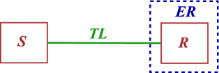
Figure 1: The communication line including the sender $S$, receiver $R$ (embedded into the extended receiver $ER$) and transmission line.

The spin dynamics is governed by the XX-Hamiltonian with the dipole-dipole interaction:

$$H = \sum_{j>i}{D_{ij}(I_{ix}I_{jx}+I_{iy}I_{jy})},$$ (14)

$$[H,I_{z}]=0,\;\;\;I_{z}=\sum_{i}{I_{iz}},$$

where $D_{ij}={\gamma^{2}\hbar}/{r_{ij}^{3}}$ is the coupling constant between the $i$th and $j$th nodes,$\gamma$ is the gyromagnetic ratio, $r_{ij}$ is the distance between the $ith$ and $jth$ nodes, $I_{i\alpha}(\alpha=x,y,z)$ is the projection operator of the $i$th spin on the $\alpha$-axis. Due to the commutation condition (14), the XX-Hamiltonian conserves the excitation number in a system and therefore has the block diagonal form (2) which, in our case of (0,1)-excitation spin dynamics, reduces to two blocks:

$$H={\mbox{diag}}(0,H_{1}).$$ (15)

The appropriate evolution operator $V(t)=e^{-iHt}$ has also the block-diagonal form,

$$V(t)={\mbox{diag}}(1,V^{(1)}),\;\;\;V^{(1)}(t)=e^{-i\frac{H^{(1)}}{D_{12}}\tau},\;\;\tau=D_{12}t,$$ (16)

where $\tau$ is the dimensionless time. At some time instant $\tau$, we apply a unitary transformation $U(\varphi)$ (which involves the set of free parameters $\varphi=\{\varphi_{1},\varphi_{2},\dots\}$) to the extended receiver. This transformation must conserve the excitation number, similarly to $V(t)$, i.e.,

$$[I_{z}^{ER},U(\phi)]=0\;\;\;\Rightarrow\;\;U={\mbox{diag}}(1,U^{(1)}),$$ (17)

where $I_{z}^{ER}$ is the $z$-projection of the total spin moment in the state-space of the extended receiver $ER$. Thus, the total transformation $W$ of the initial state is also a block-diagonal unitary transformation:

$$W(\tau) = \Big{(}I_{R,\overline{TL}}\otimes U\Big{)}V(\tau)={\mbox{diag}}(1,W^{(1)}(\tau)),$$ (22)

$$W^{(1)}=\left(\begin{array}[]{ccc}W^{(1)}_{11}&\cdots&W^{(1)}_{1N}\cr\cdots&\cdots&\cdots\cr W^{(1)}_{N1}&\cdots&W^{(1)}_{NN}\end{array}\right)$$

where $I_{R,\overline{TL}}$ is the identity matrix in the space $R\cup\overline{TL}$, $\overline{TL}$ means the $TL$ without nodes of the $ER$.

We represent $U^{(1)}$ in the exponential form,

$$U^{(1)}(\varphi)=\prod_{j=1}^{N^{(ER)}(N^{(ER)}-1)}e^{iA_{j}(\varphi_{j})},\;\;A_{j}^{\dagger}=A_{j},$$ (23)

where each $A_{j}$ is the $N^{(ER)}\times N^{(ER)}$ Hermitian off-diagonal matrix which involves only two nonzero elements introducing the real parameter $\varphi_{j}$. There are $N^{(ER)}(N^{(ER)}-1)$ linearly independent matrices of this type and the same number of the real parameters $\varphi$,

$$\varphi=\{\varphi_{i}:\;i=1,\dots,N^{(ER)}(N^{(ER)}-1)\},$$ (24)

in the unitary transformation $U^{(1)}$. Details of such parametrization are given in Z_2018 .

We consider the following tensor-product initial state

$$s=\rho^{(S)}(0)\otimes\rho^{(TL,R)}(0),$$ (25)

where $\rho^{(S)}(0)$ is an arbitrary $(0,1)$-excitation space of $N^{(S)}$-qubit sender and $\rho^{(TL,R)}(0)$ is the initial state of the joined subsystem $TL\cup R$ which is a $0$-excitation state:

$$\rho^{(TL,R)}(0)=|0\rangle_{R,TL}\;{}_{R,TL}\langle 0|.$$ (26)

The density matrix of the receiver at some time instant $\tau$ is obtained from $\rho$ by partial tracing over $S$ and $TL$:

$$r(\tau)=Tr_{S,TL}\big{(}\rho(\tau)\big{)}=Tr_{S,TL}\big{(}W(\tau)\rho(0)W^{\dagger}(\tau)\big{)}.$$ (27)

Both initial sender’s state and the receiver’s state have similar structures (compare with (7) and (12)):

$$s = \left(\begin{array}[]{c|ccc}s^{(0)}_{00}&s^{(1)}_{01}&\cdots&s^{(1)}_{0N^{(S)}}\cr\hline\cr s^{(-1)}_{10}&s^{(0)}_{11}&\cdots&s^{0}_{1N^{(S)}}\cr\cdots&\cdots&\cdots&\cdots\cr s^{(-1)}_{N^{(S)}0}&s^{(0)}_{N^{(S)}1}&\cdots&s^{0}_{N^{(S)}N^{(S)}}\end{array}\right),\;\;$$ (32)

$$r(\tau) = \left(\begin{array}[]{c|ccc}r^{(0)}_{00}(\tau)&r^{(1)}_{01}(\tau)&\cdots&r^{(1)}_{0N^{(R)}}(\tau)\cr\hline\cr r^{(-1)}_{10}(\tau)&r^{(0)}_{11}(\tau)&\cdots&r^{0}_{1N^{(R)}}(\tau)\cr\cdots&\cdots&\cdots&\cdots\cr r^{(-1)}_{N^{(R)}0}(\tau)&r^{(0)}_{N^{(R)}1}(\tau)&\cdots&r^{0}_{N^{(R)}N^{(R)}}(\tau)\end{array}\right),$$

$$r^{(0)}_{ij}=\rho^{(R)}_{N-N^{(R)}+i,N-N^{(R)}+j},\;\;i,j=1,\dots,N^{(R)},\;\;r^{(0)}_{00}=\rho^{(R)}_{00},$$

$$r^{(1)}_{0j}=\rho^{(R)}_{0,N-N^{(R)}+j},\;\;r^{(-1)}_{j0}=\rho^{(R)}_{N-N^{(R)}+j,0},\;\;j=1,\dots,N^{(R)},$$

and we set $N^{(S)}=N^{(R)}$ hereafter. We see that both $s$ and $r$ include $0$- and $\pm 1$-order coherence matrices.

III Quantum state restoring

Now we study the problem of state restoring FPZ_2021 in the case of $(0,1)$-excitation evolution in more details. We rewrite the definition (1) of the restored state for the $n$-order coherence matrices, $n=0,\pm 1$:

$$r^{(n)}_{ij}(t_{0})=\lambda^{(n)}_{ij}s^{(n)}_{ij},\;\;n=-1,0,1.$$ (38)

where the parameters $\lambda^{(n)}_{ij}$ are defined by the Hamiltonian and time instant $t_{0}$, but do not depend on the elements of $s$ and therefore they are universal for a given model of the communication line FPZ_2021 .

It was shown in the case of complete state space Z_2018 that there is a problem in restoring the diagonal elements of the density matrix. However, in the case of $(0,1)$-excitation spin dynamics this problem reduces to only one element $r^{(0)}_{00}$, which can not be restored. Moreover, we show that restoring the elements of the 1-order coherence matrix $r^{(1)}_{ij}$ automatically restores the elements $s^{(0)}_{ij}$, $i,j\neq 0$. Of course, the elements of $r^{(-1)}$ becomes also restored since $r^{(-1)}=\Big{(}r^{(1)}\Big{)}^{\dagger}$.

We start with writing the explicit relations between the elements of $r$ and $s$. For that, we label the elements of $W^{(1)}$ by a triple index $\{n,m,l\}$, where the first, second and third indexes are withing the intervals, respectively, $0\leq n\leq N^{(S)}$, $0\leq m\leq N^{(TL)}$, $0\leq l\leq N^{(R)}$. Here $N^{(S)}$, $N^{(TL)}$ and $N^{(R)}$ are, respectively, the numbers of nodes in the sender, transmission line and receiver. Then Eq.(27) yields

$$r^{(0)}_{00} = s^{(0)}_{00}+\sum_{{n,m}\atop{|n|+|m|=1}}\sum_{j,k=1}^{N^{(S)}}W^{(1)}_{n,m,0;j,0,0}s^{0}_{jk}(W^{(1)})^{\dagger}_{k,0,0;n,m,0},$$ (39)

$$r^{(1)}_{0n} = \sum_{j=1}^{N^{(S)}}s^{(1)}_{0j}(W^{(1)})^{\dagger}_{j,0,0;0,0,n},$$ (40)

$$r^{(0)}_{nm} = \sum_{j,k=1}^{N^{(S)}}W^{(1)}_{0,0,n;j,0,0}s^{0}_{jk}(W^{(1)})^{\dagger}_{k,0,0;0,0,m},\;\;n,m\neq 0.$$ (41)

We see that restoring $r^{(1)}$ requires the ”diagonal” form for $W^{(1)}_{0,0,n;j,0,0}$:

$$W^{(1)}_{0,0,n;j,0,0}=\lambda^{(1)}_{n0}\delta_{nj}.$$ (42)

This means that we have to find such parameters $\varphi$ of the unitary transformation $U^{(1)}$ that solve the following system of $N^{(S)}(N^{(S)}-1)$ complex equations

$$W^{(1)}_{0,0,n;j,0,0}=0,\;\;n\neq j,$$ (43)

which is equivalent to the system of

$$2N^{(S)}(N^{(S)}-1)$$ (44)

real equations. Comparison of (24) and (44) yields the condition on the lower bound for $N^{(ER)}$:

$$N^{(ER)}(N^{(ER)}-1)>2N^{(S)}(N^{(S)}-1).$$ (45)

By virtue of (43), system (39) - (41) takes the following form

$$r^{(0)}_{00} = s^{(0)}_{00}+\sum_{{m=1}\atop{mn=0}}^{N^{(TL)}}\sum_{n,j=1}^{N^{(S)}}|W^{(1)}_{n,m,0;j,0,0}|^{2}s^{0}_{jj},$$ (46)

$$r^{(1)}_{0n} = (\lambda^{(1)}_{n0})^{*}s^{(1)}_{0n},$$ (47)

$$r^{(0)}_{nm} = \lambda^{(1)}_{n0}(\lambda^{(1)}_{m0})^{*}s^{0}_{nm},\;\;n,m>0,\;\;\Rightarrow\;\;\lambda^{(0)}_{nm}=\lambda^{(1)}_{n0}(\lambda^{(1)}_{m0})^{*},$$ (48)

where $*$ means the complex conjugate. Deriving (46) we use the unitarity of $W^{(1)}$.

IV Entanglement in (0,1)-excitation state restoring

We consider two measures of entanglement.

The first one is the measure of bi-qubit entanglement. We calculate the entanglement between any two qubits of the sender and its evolution to the entanglement between corresponding two qubits of the receiver. Using the Wootters criterion HW ; Wootters with the concurrence as a measure of quantum entanglement we show that the evolution of the concurrence reduces to its scaling with the scale factor independent on the initial sender’s state.

The second measure of entanglement is the double negativity (PPT-criterion) Peres ; VW . It measures the bi-partite entanglement between two multiqubit (in general) systems which are sender and receiver in our case.

IV.1 Scaling of pairwise entanglement

We calculate the quantum entanglement by the Wootters criterion using the following formula HW ; Wootters :

$$C(r) = \max(0;\lambda_{1}-\lambda_{2}-\lambda_{3}-\lambda_{4}),$$ (49)

$$R = \sqrt{r(\sigma_{y}\otimes\sigma_{y})r^{*}(\sigma_{y}\otimes\sigma_{y})},\;\;\sigma_{y}=\left(\begin{array}[]{cc}0&-i\cr i&0\end{array}\right).$$ (52)

Here $\lambda_{i},i=1,...,4$ are eigenvalues of the matrix $R$ and $\lambda_{1}$ is the biggest of them.

Consider the $(0,1)$-excitation density matrix $s$ (32). To calculate the concurrence between the $i$th and $j$th spins we have to calculate the partial trace of $s$ with respect to all spins except the $i$th and $j$th to obtain the two-qubit density matrix $s^{(ij)}$, which we have to represent in the two-qubit basis

$$|00\rangle,\;\;|01\rangle,\;\;|10\rangle,\;\;|11\rangle.$$ (53)

This matrix reads:

$$s^{(ij)}=\left(\begin{array}[]{cccc}s_{00}&s_{0i}&s_{0j}&0\cr s_{0i}^{*}&s_{ii}&s_{ij}&0\cr s_{0j}^{*}&s_{ij}^{*}&s_{jj}&0\cr 0&0&0&0\end{array}\right),\;\;i,j>0.$$ (58)

It is remarkable that the nonzero eigenvalues of the matrix $R$ (52) read

$$\lambda_{1}=\sqrt{s_{ii}s_{jj}}+|s_{ij}|,\;\;\lambda_{2}=\sqrt{s_{ii}s_{jj}}-|s_{ij}|,$$ (59)

where we take into account the non-negativity of the density matrix $s$, so that

$$s_{ii}s_{jj}-|s_{ij}|^{2}\geq 0.$$ (60)

Then, concurrence between the $i$th and $j$th nodes of the sender reads

$$C_{ij}^{(s)}=2|s_{ij}|,\;\;i\neq j.$$ (61)

We shall emphasize that the concurrence does not depend on the elements of the $\pm 1$-order coherence matrices of $s^{(ij)}$. Thus we proved the following Proposition.

Proposition 1. The concurrence of 2-qubit state (58) is defined by the single element of the density matrix $s$ by formula (61).

Proposition 2. If all non-diagonal elements in the 0-order coherence matrix $r^{(0)}$ of state $r$ (II) are proportional to the appropriate elements of $s^{(0)}$ of state $s$ (32) according to (38), then

$$\frac{C^{(r)}_{ij}}{C^{(s)}_{ij}}=2|\lambda^{(0)}_{ij}|=2|\lambda^{(1)}_{i}(\lambda^{(1)}_{j})^{*}|,\;\;\forall\;i,j,\;\;i\neq j.$$ (62)

It is important that relation (62) holds for all pairs $(i,j)$ of different spins of the sender (and receiver) in the case of state restoring. Therefore, the long-distance state restoring scales the pairwise concurrence with the universal (i.e., independent on the sender’s initial state $s$) scale parameter $2|\lambda^{(0)}_{ij}|$. This scale parameter is defined by the Hamiltonian which governs the spin dynamics, and by the time instant $\tau$ selected for state registration.

IV.2 $S-R$ entanglement via PPT criterion

The Wootters criterion is well applicable for calculating the 2-qubit entanglement. However, to calculate the entanglement between two multi-qubit subsystems another method must be implemented. We consider the PPT criterion Peres ; VW for this purpose. According to this criterion, the entanglement between two quantum subsystems $S$ and $R$ of system is expressed in terms of the so-called double negativity $N_{SR}$, which is the doubled sum of the absolute values of the negative eigenvalues $\lambda_{i}<0$ of the matrix $(\rho^{(RS)})^{T_{S}}$,

$$N_{SR}=2\sum_{\lambda_{i}<0}|\lambda_{i}|.$$ (63)

Here

$$\rho^{(RS)}(\tau)={\mbox{Tr}}_{TL}\;\rho(\tau),$$ (64)

and the superscript $T_{S}$ means the partial transpose with respect to the subsystem $S$.

V Examples: structural restoring of 2- and 3-qubit states.

V.1 Time instant for state registration.

First, we fix the time instant $\tau$ that maximizes the minimal of the scale parameters $\lambda^{(1)}_{i0}$, $i=1,\dots,N^{(S)}$, which we denote $\lambda(N)$. At that, we fix the optimal parameters $\varphi$ obtained as solutions of Eq.(43). In other words, we define the parameter $\lambda(N)$ according to the following scheme.

1. For each chain length $N$, we scan the time interval $0\leq\tau\leq T\gtrsim N$.

2. At each $\tau$-instant, we find 1000 independent solutions $\varphi^{(i)}(\tau)$ of (43), $i=1,\dots,1000$.

3. For each solution $\varphi^{(i)}(\tau)$, we calculate $\lambda^{(1)}_{j0}(\tau,\varphi^{(i)})\equiv\lambda^{(1;i)}_{j0}$, $j=1,\dots,N^{(S)}$.

4. Find $\lambda_{min}^{(i)}(\tau)=\min\Big{(}\lambda^{(1;i)}_{1}(\tau),\dots,\lambda^{(1;i)}_{N^{(S)}}(\tau)\Big{)}$.

5. Then

   $$\lambda(N)=\max_{\tau,i}\;\lambda_{min}^{(i)}(\tau).$$ (65)

   We denote the time instant yielding maximum in (65) by $\tau(N)$.

V.2 Two-qubit state restoring.

We consider the two-qubit receiver ($N^{(S)}=N^{(R)}=2$) with the three-qubit extended receiver ($N^{(ER)}=3$). In the above protocol of calculating $\lambda(N)$, we include the set of 1000 solutions $\varphi^{(i}$ of system (43), ${i=1,\dots,1000}$. The graphs $\lambda(N)$ and $\tau(N)$ are shown in Fig.2. Notice that $\tau(N)$ appears to be a straight line.

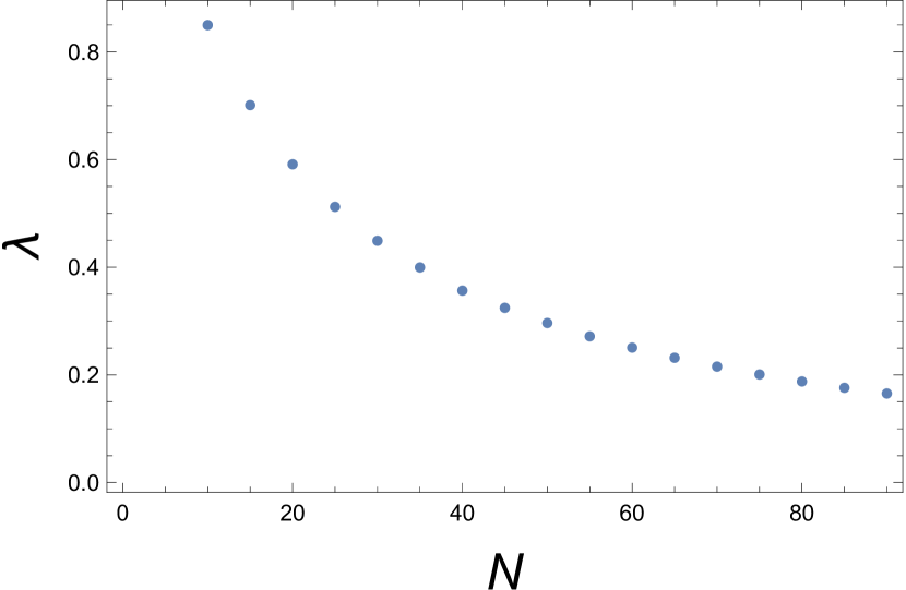
(a)

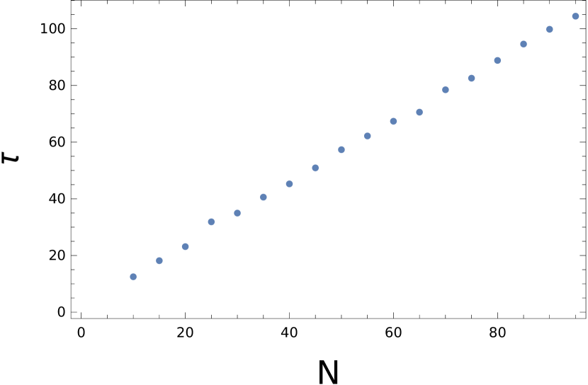
(b)

Figure 2: The parameters $\lambda(N)$ (a) and $\tau(N)$ (b) as functions of the chain length $N$ for $N^{(S)}=2$, $N^{(EX)}=3$.

Let us consider a particular example of two-qubit state restoring in the communication line of $N=10$ nodes. An optimized unitary transformation at ${\tau=12.5}$ reads

$$U^{(1)}=\left(\begin{array}[]{cccc}0.008e^{i2.790}&0.967e^{-i3.109}&0.052e^{i1.132}&0.249e^{i3.058}\cr 0.819e^{i2.649}&0.027e^{-i1.903}&0.530e^{-i2.974}&0.215e^{i1.511}\cr 0.195e^{-i2.276}&0.249e^{i2.015}&0.264e^{i2.015}&0.911e^{-i2.031}\cr 0.538e^{-i1.225}&0.039e^{-i1.332}&0.804e^{i1.470}&0.249e^{i1.001}\end{array}\right).$$ (70)

Corresponding matrix $r$ reads

$$r=\left(\begin{array}[]{ccc}r_{00}&0.655e^{-i0.094}s_{01}&0.584e^{i1.783}s_{02}\cr 0.655e^{i0.094}s_{01}^{*}&0.429s_{11}&0.382e^{i1.876}s_{12}\cr 0.584e^{-i1.783}s_{02}^{*}&0.382e^{-i7.876}s_{12}^{*}&0.341s_{22}\cr\end{array}\right),$$ (74)

$$\lambda^{(1)}_{1}=0.655e^{-i0.094},\;\;\lambda^{(1)}_{2}=0.5834e^{i1.783}.$$

where $r_{00}=s_{00}+0.571s_{11}+0.659s_{22}$.

Now we turn to the bi-particle entanglement. To illustrate the dependence of the ratio $C^{(r)}_{12}/C^{(s)}_{12}$ on the solution $\varphi^{(i)}$ of system (43), we plot $C^{(r)}_{12}/C^{(s)}_{12}$ for different solutions $\varphi^{(i)}$, $i=1,\dots,1000$ and chain length ${N=10}$ at ${\tau=12.5}$, see Fig.3. The maximal value of this ratio is 0.752. The maximal density of the points on Fig.3 is observed at $C^{(r)}_{12}/C^{(s)}_{12}\sim 0.1\div 0.3$.

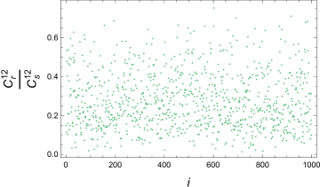
Figure 3: The ratio $C^{(r)}_{12}/C^{(s)}_{12}$ in dependence on number of solution $\varphi^{(i)}$, $i$; the maximal value of this ratio equals 0.752.

V.3 3-qubit state restoring.

As another example, we investigate and optimize (over 1000 solutions $\varphi^{(i)}$ of system (43)) of the ratios $C^{(r)}_{ij}/C^{(s)}_{ij}=2|\lambda^{(0)}_{ij}|$ for three possible pairs of spins in a three-qubit receiver and sender. The length of the chain is $N=10$, the extended receiver includes $5$ qubits. The time corresponding to the maximal ratio (or maximal $|\lambda^{(0)}_{ij}|$) is found for each pair of qubits. The results are collected in Table 1.

$\{i,j\}$	$\tau$	$C^{(r)}_{ij}/C^{(s)}_{ij}$
{1,2}	110	0.092
{2,3}	108.5	0.054
{1,3}	109.4	0.025

Table 1: The ratio $C^{(r)}_{ij}/C^{(s)}_{ij}$ maximized over 1000 $\varphi^{(i)}$ and over time. The optimal time instant $\tau$ for each pair $\{i,j\}$ is given.

V.3.1 $S-R$ entanglement via PPT criterion.

Now we strive to maximize entanglement between $S$ and $R$ for this example using the PPT criterion (double negativity $N_{SR}$ is a measure of entanglement). First, for each $\tau$, $0\leq\tau\leq 2N=20$, we optimize $\varphi$ calculating $\lambda(N)$, $N=10$, (see Eq.(65)) with maximization over 500 solutions $\varphi^{(i)}$, $i=1,\dots,500$ of system (43). Then, for the optimized $\varphi$, we calculate double negativity $N_{SR}$ averaged over $200$ pure sender’s initial states taken in the form

$$|\Psi^{(S)}\rangle = \sum_{i=0}^{3}a_{i}|i\rangle,$$

$$a_{0}=\cos\,\psi_{1}\;\cos\,\psi_{2}\;\cos\,\psi_{3},$$

$$a_{1}=\sin\,\psi_{1}\;\cos\,\psi_{2}\;\cos\,\psi_{3}\;e^{i\phi_{1}}$$

$$a_{2}=\sin\,\psi_{2}\;\cos\,\psi_{3}\;e^{i\phi_{2}}$$

$$a_{3}=\sin\,\psi_{3}\;e^{i\phi_{3}},$$

where $\psi_{i}$ and $\phi_{i}$ are randomly chosen real parameters. The graph of $N_{SR}$ as a function of $\tau$ calculated in this way is shown on Fig.4. Two maxima at $\tau\sim 10$ and $\tau\sim 18$ are observed.

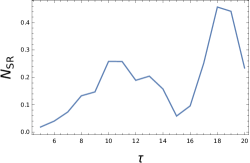
Figure 4: The $\tau$-dependence of the double negativity averaged over 200 arbitrary pure initial states (V.3.1).

The distribution of double negativity $N_{SR}$ for 100 random sender’s initial states at $\tau=18$ (the second maximum on Fig.4) is shown in Fig.5 with the maximal value is $N_{SR}=0.935$

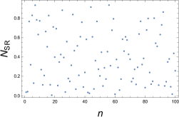
Figure 5: The diagram of $S-R$ entanglement in dependence on different sender’s initial states numbered by $n$ at $\tau=18$; the maximal value of this ratio equals $N_{SR}=0.935$.

VI Conclusions

We consider the process of remote structural state restoring of (0,1)-excitation states (i.e., states including only 0- and 1-excitations). We show, that in this case almost complete structural state restoring can be performed by restoring only the 1-order coherence matrix. At that, the only non-restorable element of the density matrix is the element from the 0-excitation block of 0-order coherence matrix.

We study the entanglement in this process and find out that the concurrence between any two sender’s qubits scales to the concurrence between the corresponding two qubits of the receiver. It is remarkable that the factor of such scaling is universal, i.e., it does not depend on the particular sender’s state. This factor is defined by the Hamiltonian and time instant for state registration. Examples of 2 and 3-qubit state restoring are presented.

Two above results (almost complete structural state restore and scaled concurrence) can be referred to the features of (0,1)-excitation evolution which can not be observed in the case of evolution in the complete state space.

The entanglement between the sender and receiver is studied using the PPT-criterion (doble negativity). In this case we consider the $N=10$ chain with 3-qubit receiver (sender) and average the double negativity over 200 random initial pure states of the sender. We define the maxima at $\tau\sim 10$ ($\sim N$) and $\tau\sim 18$ ($\sim 2N$).

Acknowledgments. The work was performed as a part of a state task, State Registration No. AAAA-A19-119071190017-7.

References

• (1) Bose S. Quantum communication through an unmodulated spin chain, Phys. Rev. Lett. 91 (2003) 207901
• (2) Christandl M., Datta N., Ekert A., and Landahl A.J. Perfect state transfer in quantum spin networks, Phys.Rev.Lett. 92 (2004) 187902
• (3) Karbach P., and Stolze J. Spin chains as perfect quantum state mirrors, Phys.Rev.A. 72 (2005) 030301(R)
• (4) Gualdi G., Kostak V., Marzoli I., and Tombesi P. Perfect state transfer in long-range interacting spin chains, Phys.Rev. A. 78 (2008) 022325
• (5) De Chiara G., Rossini D., Montangero S., and Fazio R. From perfect to fractal transmission in spin chains, Phys. Rev. A. 72 (2005) 012323
• (6) Zwick A., Álvarez G.A., Stolze J., Osenda O. Robustness of spin-coupling distributions for perfect quantum state transfer, Phys. Rev. A. 84 (2011) 022311
• (7) Zwick A. , Álvarez G.A., Stolze J., and Osenda O. Spin chains for robust state transfer: Modified boundary couplings versus completely engineered chains, Phys. Rev. A. 85 (2012) 012318
• (8) Zwick A., Álvarez G.A. , Stolze J., and Osenda O. Quantum state transfer in disordered spin chains: How much engineering is reasonable? Quant. Inf. Comput. 15(7-8), (2015) 582
• (9) Peters N.A., Barreiro J.T., Goggin M.E., Wei T.-C., and Kwiat P.G. Remote State Preparation: Arbitrary Remote Control of Photon Polarization, Phys.Rev.Lett. 94, (2005) 150502
• (10) Peters N.A., Barreiro J.T., Goggin M.E., Wei T.-C., and Kwiat P.G. Remote State Preparation: Arbitrary remote control of photon polarizations for quantum communication, Quantum Communications and Quantum Imaging III, ed. R.E.Meyers, Ya.Shih. Proc. of SPIE 5893 SPIE. Bellingham. WA. (2005)
• (11) Dakic B. , Lipp Ya.O., Ma X., Ringbauer M., Kropatschek S., Barz S., Paterek T., Vedral V., Zeilinger A., Brukner C., and Walther P. Quantum discord as resource for remote state preparation, Nat. Phys. 8, (2012) 666
• (12) Pouyandeh S., Shahbazi F., Bayat A. Measurement-induced dynamics for spin-chain quantum communication and its application for optical lattices, Phys.Rev.A. 90, (2014) 012337
• (13) Liu L.L., and Hwang T. Controlled remote state preparation protocols via AKLT states, Quant.Inf.Process. 13 (2014) 1639
• (14) E.B. Fel’dman, A.N. Pechen, A.I. Zenchuk, Complete structural restoring of transferred multi-qubit quantum state, Phys.Lett. A 413 (2021) 127605
• (15) E.B.Fel’dman and A.I.Zenchuk Coherence Evolution and Transfer Supplemented by Sender’s Initial-State Restoring, JETP 125(6), (2017) 1042
• (16) A.I. Zenchuk, Partial structural restoring of two-qubit transferred state, Phys.Lett.A 382 (2018) 3244
• (17) G.A.Bochkin, E.B.Fel’dman, I.D.Lazarev, A.N.Pechen, A.I.Zenchuk, Transfer of zero-order coherence matrix along spin-1/2 chain, Quant.Inf.Proc. 21 (2022) 261,
• (18) S.Hill, and W.K.Wootters, Entanglement of a pair of quantum bits, Phys.Rev.Lett. 78, 5022 (1997)
• (19) W.K.Wootters, Entanglement of formation of an arbitrary state of two qubits, Phys.Rev.Lett. P80, 2245 (1998)
• (20) A.Peres, Separability criterion for density matrices, Phys.Rev.Lett. 77, 1413 (1996)
• (21) G.Vidal, and R.F.Werner, Computable measure of entanglement, Phys.Rev.A. 65, 032314 (2002)