Lie Neurons: Adjoint-Equivariant Neural Networks for Semisimple Lie Algebras

Abstract

This paper proposes an equivariant neural network that takes data in any semi-simple Lie algebra as input. The corresponding group acts on the Lie algebra as adjoint operations, making our proposed network adjoint-equivariant. Our framework generalizes the Vector Neurons, a simple $\mathrm{SO}(3)$-equivariant network, from 3-D Euclidean space to Lie algebra spaces, building upon the invariance property of the Killing form. Furthermore, we propose novel Lie bracket layers and geometric channel mixing layers that extend the modeling capacity. Experiments are conducted for the $\mathfrak{so}(3)$ and $\mathfrak{sl}(3)$ Lie algebras on various tasks, including fitting equivariant and invariant functions, learning system dynamics, point cloud registration, and homography-based shape classification. Our proposed equivariant network shows wide applicability and competitive performance in various domains.

Equal contribution

1 Introduction

For geometric problems in control theory, robotics, computer vision and graphics, Lie group methods provide the machinery to study continuous symmetries inherent to the problem (Murray et al., 1994; Liu et al., 2010; Lynch & Park, 2017; Barrau & Bonnabel, 2017; van Goor et al., 2020; Yang et al., 2021; Lin et al., 2022; Ghaffari et al., 2022). Lie algebras are vector spaces that locally preserve the group structure, enabling efficient computation (Teng et al., 2022; Lin et al., 2023b). The standard group representation (linear group action) on Lie algebras is given by conjugation or adjoint action (Hall, 2013).

The equivariance property preserves the symmetry group structure, often a Lie group, such that the feature map commutes with the group representation. Equivariant models have gained success in various domains, including but not limited to the modeling of molecules (Thomas et al., 2018), physical systems (Finzi et al., 2020), social networks (Maron et al., 2018), images (Worrall et al., 2017), and point clouds (Zhu et al., 2023b). Convolutional neural networks (CNNs) are translation-equivariant, enabling stable image features regardless of the pixel positions in the image plane. Typical extensions include rotation (Cohen et al., 2017) and scale (Worrall & Welling, 2019) equivariance, while more general extensions are also explored (MacDonald et al., 2022).

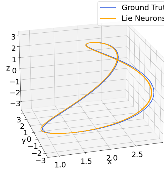
(a)

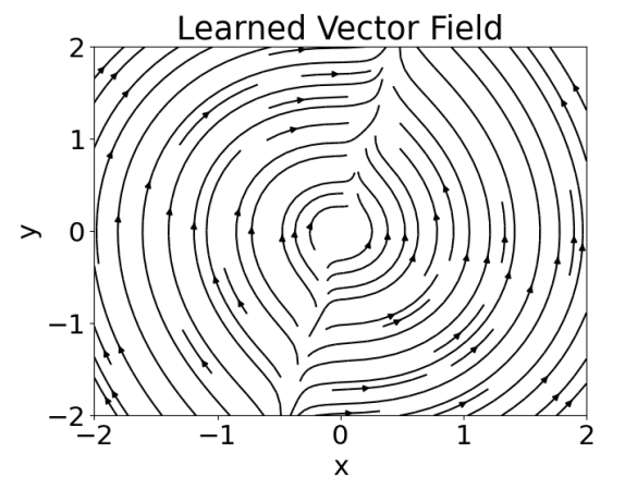
(b)

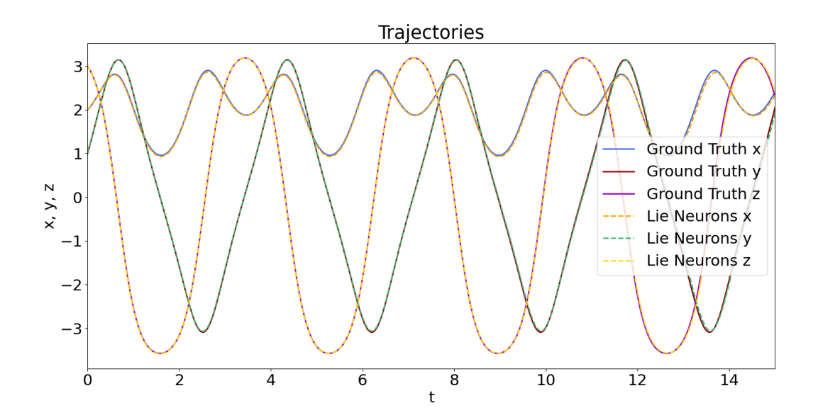
(c)

Figure 1: The Lie Neurons can be applied in learning dynamics. In this example, we learn the dynamics of a simulated free-rotation International Space Station, which we pose as an initial value problem in the Neural ODE framework. This figure shows the estimated trajectories and the learned vector field from the Lie Neurons. Detail descriptions can be found in Section 5.1.2.

In this paper, we propose a new type of equivariant model that captures the symmetry in Lie algebra spaces. For a given Lie algebra, we represent its elements as vectors by specifying a set of bases, and represent the adjoint actions as matrix multiplications, exploiting the isometry structure of Lie algebras to handle such data in typical vector form. Through the connection between inner products and the Killing form, we generalize the architecture of Vector Neurons (Deng et al., 2021), a $\mathrm{SO}(3)$-equivariant network originally designed for point cloud data in 3-D Euclidean space, to process data in arbitrary semisimple Lie algebra. We further build new types of equivariant network layers that exploit the structure of Lie algebras and extend the flexibility of the model. Using $\mathfrak{so}(3)$ and $\mathfrak{sl}(3)$ as examples, we conduct experiments on various tasks in physics, computer vision, and general function fitting, and show that our proposed network has wide applicability and competitive performance.

In particular, the contributions of this work are as follows.

1. We propose a new adjoint-equivariant network architecture, enabling the processing of semisimple Lie algebraic input data. Such models frequently appear in real-world geometric problems.

2. We develop new network designs using the Killing form and the Lie bracket structure for equivariant activation and invariant layers for Lie algebraic representation learning.

3. We propose equivariant channel mixing layers that enable fusing information across the geometric dimension, which was not possible in the previous work (Deng et al., 2021).

4. The software implementation can be found at https://github.com/UMich-CURLY/LieNeurons.

2 Related Work

Equivariant networks enable the model output to change in a predicted way as the input goes through certain transformations. This means that the model, by construction, generalizes over the variations caused by those transformations. Therefore, it reduces the sampling complexity in learning and improves the robustness and transparency facing input variations. (Cohen & Welling, 2016a) initials the idea to generalize equivariance in deep learning models, realizing equivariance to 90-degree rotations in a 2D image plane using group convolution. This method works with discrete transformations by augmenting the input domain with a dimension for the set of transformations. The approach is generalized to other discretized groups in $SE(2)$, $SE(3)$, and $E(3)$ (Hoogeboom et al., 2018; Winkels & Cohen, 2018; Worrall & Brostow, 2018; Chen et al., 2021; Zhu et al., 2023a). Steerable convolution is proposed in (Cohen & Welling, 2016b), leveraging the irreducible representations to remove the need for discretization and facilitate equivariant convolution on continuous groups in the frequency domain (Worrall et al., 2017; Cohen et al., 2017; Weiler et al., 2018). Beyond convolutions, more general equivariant network architectures are proposed, for example, (Fuchs et al., 2020; Hutchinson et al., 2021; Chatzipantazis et al., 2022) for transformers and (Batzner et al., 2022; Brandstetter et al., 2021) for message passing networks. Vector Neurons (Deng et al., 2021) designs a multi-layer perception (MLP) and graph network that generalize the scalar features to 3D features to realize $\mathrm{SO}(3)$-equivariance on spatial data. The above works mainly focus on compact groups, on which more general recipes for building equivariant layers that are not limited to a specific group are also proposed (Kondor & Trivedi, 2018; Cohen et al., 2019; Weiler & Cesa, 2019; Xu et al., 2022; Lang & Weiler, 2020). The extension of equivariance beyond compact groups is also explored. (Finzi et al., 2021) constructs MLPs equivariant to arbitrary matrix groups using their finite-dimensional representations. With the Monte Carlo estimator, equivariant convolutions are generalized to matrix groups with surjective exponential maps (Finzi et al., 2020) and all finite-dimensional Lie groups (MacDonald et al., 2022), where Lie algebra is used to parameterize elements in the continuous Lie groups as a lifted domain from the input space.

Our model structure resembles the MLP style of Vector Neurons (Deng et al., 2021), but our work models the equivariance of arbitrary semisimple groups under adjoint actions. Different from Vector Neurons, the input domain of our method is the Lie algebra.

3 Preliminaries

We provide some preliminaries for Lie groups by focusing on matrix Lie groups. For detailed explanations, we refer the readers to (Hall, 2013; Rossmann, 2006; Kirillov, 2008).

3.1 Lie Group and Lie Algebra

A Lie group $\mathcal{G}$ is a smooth manifold whose elements satisfy the group axioms. Because of this, a special vector space naturally arises at the identity of every Lie group named the Lie algebra, denoted $\mathfrak{g}$. A Lie algebra locally captures the structure of the Lie group.

Every Lie algebra is equipped with an asymmetric binary operator called the Lie bracket:

$$\left[\cdot,\cdot\right]:\quad\mathfrak{g}\times\mathfrak{g}\rightarrow\mathfrak{g}.$$ (1)

The elements of the Lie algebra have non-trivial structures. However, since the Lie algebra is a vector space, for a Lie algebra of dimension $m$, we can always represent it using $\mathbb{R}^{m}$ given appropriate bases. As a result, we introduce two useful maps (Chirikjian, 2011):

$$\text{Vee}: \mathfrak{g}\rightarrow\mathbb{R}^{m},\quad x^{\wedge}\mapsto(x^{\wedge})^{\vee}=\sum^{m}_{i=1}x_{i}e_{i},\quad$$ (2)

$$\text{Hat}: \mathbb{R}^{m}\rightarrow\mathfrak{g},\quad x\mapsto x^{\wedge}=\sum^{m}_{i=1}x_{i}E_{i},$$ (3)

where $e_{i}$ are the canonical basis of $\mathbb{R}^{m}$ and $E_{i}=(e_{i})^{\wedge}\in\mathfrak{g}$.

For example, the $\mathfrak{so}(3)$ elements are skew-symmetric, $\begin{bmatrix}0&-\omega_{z}&\omega_{y}\\ \omega_{z}&0&-\omega_{x}\\ -\omega_{y}&\omega_{x}&0\end{bmatrix}\in\mathfrak{so}(3)$. One can find the canonical basis as follows:

$$\small E_{x}=\begin{bmatrix}0&0&0\\ 0&0&-1\\ 0&1&0\end{bmatrix},E_{y}=\begin{bmatrix}0&0&1\\ 0&0&0\\ -1&0&0\end{bmatrix},E_{z}=\begin{bmatrix}0&-1&0\\ 1&0&0\\ 0&0&0\end{bmatrix}.$$ (4)

Using the Hat and Vee maps, we can represent an element of the Lie algebra in a neural network using $\mathbb{R}^{m}$, while performing structure-preserving operations on $\mathfrak{g}$. In this work, we use the basis of $\mathfrak{so}(3)$ in (4), and $\mathfrak{sl}(3)$ from (Winternitz, 2004) to construct the Hat and Vee maps.

3.2 Adjoint Representation

Given an element of the Lie algebra $X\in\mathfrak{g}$ and its corresponding Lie group $\mathcal{G}$, every $a\in\mathcal{G}$ defines an automorphism of the Lie algebra $Ad_{a}:\mathfrak{g}\rightarrow\mathfrak{g}$ by $Ad_{a}(X)=aXa^{-1}$. This is called the adjoint action of the group $\mathcal{G}$ on the Lie algebra $\mathfrak{g}$. It represents the change of basis operations on the algebra. Since the adjoint $Ad_{a}$ is linear, we can find a matrix that maps the $\mathbb{R}^{m}$ representation of the Lie algebra to another. That is, for every $Ad_{a}$ and $X\in\mathfrak{g}$, we have

$$Adm_{a}:\quad\mathbb{R}^{m}\rightarrow\mathbb{R}^{m},\quad x\mapsto Adm_{a}x,$$ (5)

with $Adm_{a}\in\mathbb{R}^{m\times m}$, $x=X^{\vee}$ and $Adm_{a}x=(aXa^{-1})^{\vee}$. This is an important property as it allows us to model the group adjoint action using a matrix multiplication on $\mathbb{R}^{m}$, which enables the adjoint equivariant layer design in Section 4.

This work focuses on the matrix Lie group, where the Lie bracket is defined by the commutator: $\left[X,Y\right]=XY-YX$. It is worth noticing that the Lie bracket is equivariant under the group adjoint action, i.e., $\left[Ad_{a}(X),Ad_{a}(Y)\right]=Ad_{a}(\left[X,Y\right]),\forall a\in\mathcal{G}$.

3.3 Killing Form

If a Lie algebra $\mathfrak{g}$ is of finite dimension and associated with a field $\mathbb{R}$, a symmetric bilinear form called the Killing form is defined as:

$$B(X,Y):\mathfrak{g}\times\mathfrak{g}\rightarrow\mathbb{R},\quad(X,Y)\mapsto\operatorname{tr}(ad_{X}\circ ad_{Y})$$ (6)

Definition 3.1.

A bilinear form $B(X,Y)$ is said to be non-degenerate iff $B(X,Y)=0$ for all $Y\in\mathfrak{g}$ implies $X=0$.

Theorem 3.2 ((Kirillov, 2008)).

A Lie algebra is semisimple iff the Killing form is non-degenerate.

Theorem 3.3 ((Kirillov, 2008)).

The Killing form is invariant under the group adjoint action $Ad_{a}$ for all $a\in\mathcal{G}$, i.e.,

$$B(Ad_{a}(X),Ad_{a}(Y))=B(X,Y).$$

If the Lie group is also compact, the Killing form is negative definite, and the inner product naturally arises from the negative of the Killing form.

4 Methodology

We present Lie Neurons (LN), a general adjoint-equivariant neural network on Lie algebras. It is greatly inspired by Vector Neurons (VN) (Deng et al., 2021). Vector Neurons take 3-dimensional vectors as inputs, typically viewed as points in Euclidean space. The 3D Euclidean dimension is preserved in the features (which we call the geometric dimension), independent from the feature dimension. In other words, Vector Neurons lift conventional $\mathbb{R}^{C}$ features in an MLP to $\mathbb{R}^{3\times C}$, allowing the same $\mathrm{SO}(3)$ actions to be applied in the input space and the feature space, facilitating the equivariance property.

The Lie Neurons generalize VN with 3-channel geometric dimension to networks with $K$-channel geometric dimension, where $K$ is the dimension any semisimple Lie algebra, and the networks are equivariant to the adjoint action of the corresponding Lie group. Similar to how VN takes 3-dimensional points as input, our networks take elements of the Lie algebra as input. While a Lie algebra $\mathfrak{g}$ is a vector space with non-trivial structures, $X\in\mathfrak{g}$ can be expressed as a $K$-dimensional vector $x=X^{\vee}\in\mathbb{R}^{K}$ with appropriate bases using (2). This representation is the core concept for Lie Neurons.

Lie Neurons operate on the $\mathbb{R}^{K}$ representation of the Lie algebra. We denote the input as $\mathbf{x}\in\mathbb{R}^{K\times C}$, where $C$ is the feature dimension. This can be viewed as $C$ Lie algebra elements in the $\mathbb{R}^{K}$ form. That is, the Lie Neurons model $f:\mathfrak{g}^{C_{1}}\rightarrow\mathfrak{g}^{C_{2}}$ can be instantiated as

$$f:\mathfrak{\mathbb{R}}^{K\times C_{1}}\rightarrow\mathfrak{\mathbb{R}}^{K\times C_{2}}.$$ (7)

Recall from (5) that $Adm_{a}\in\mathbb{R}^{K\times K}$ is the matrix form of the adjoint operator such that $Adm_{a}x=(Ad_{a}(X))^{\vee}=(aXa^{-1})^{\vee}$. This means that we can represent the adjoint action as a left matrix multiplication on the input $\mathbf{x}$. The equivariance of the network can then be defined as

$$f(Adm_{a}\mathbf{x};\theta)=Adm_{a}f(\mathbf{x};\theta).$$ (8)

For a set of $N$ input elements $\{X\}_{N}$, the learned feature is $\{\mathbf{x}\}_{N}\in\mathbb{R}^{K\times C\times N}$. We will use a single element to explain the network components for simplicity, unless noted otherwise.

A Lie Neurons network can be constructed with linear layers, two types of nonlinear activation layers, geometric channel mixing layers, pooling layers, and invariant layers. We start by discussing the linear layers as follows.

4.1 Linear Layers

Linear layers are the basic building blocks of an MLP. A linear layer has a learnable weight matrix $W\in\mathbb{R}^{C\times C^{\prime}}$, which operates on input features $\mathbf{x}\in\mathbb{R}^{K\times C}$ by right matrix multiplication:

$$\mathbf{x}^{\prime}=f_{\text{LN-Lin}}(\mathbf{x};W)=\mathbf{x}W\in\mathbb{R}^{K\times C^{\prime}}.$$ (9)

A linear layer can be viewed as a matrix multiplication on the right (feature dimension $C$), which does not affect the adjoint operation as matrix multiplication on the left (geometric dimension $K$), thus preserving the equivariance property:

$$\begin{split}f_{\text{LN-Lin}}(Ad_{a}(\mathbf{x});W)&=f_{\text{LN-Lin}}(Adm_{a}\mathbf{x};W)\\ &=Adm_{a}\mathbf{x}W\in\mathbb{R}^{K\times C^{\prime}}\\ &=Adm_{a}f_{\text{LN-Lin}}(\mathbf{x};W)\\ &=Ad_{a}(f_{\text{LN-Lin}}(\mathbf{x};W)^{\wedge}),\end{split}$$ (10)

It is worth mentioning that we ignore the bias term to preserve the equivariance. Lastly, similar to the Vector Neurons, the weights may or may not be shared across the elements $\mathbf{x}$ in $\{\mathbf{x}\}_{N}$.

4.2 Nonlinear Layers

Nonlinear layers enable the neural network to approximate complicated functions. We propose two designs for the equivariant nonlinear layers, LN-ReLU and LN-Bracket.

4.2.1 LN-ReLU: Nonlinearity Based on the Killing Form

We can use an invariant function to construct an equivariant nonlinear layer. The VN leverages the inner product in a standard vector space, which is invariant to $\mathrm{SO(3)}$, to design a vector ReLU nonlinear layer. We generalize this idea by replacing the inner product with the negative of the Killing form. As described in Section 3, the negative Killing form falls back to the inner product for compact semisimple Lie groups, and it is invariant to the group adjoint action.

For an input $\mathbf{x}\in\mathbb{R}^{K\times C}$, a Killing form $B(\cdot,\cdot)$, and a learnable weight $U\in\mathbb{R}^{C\times C}$, the nonlinear layer $f_{\text{LN-ReLU}}$ is defined as:

$$f_{\text{LN-ReLU}}(\mathbf{x})=\begin{cases}\mathbf{x},&\text{if}\ B(\mathbf{x},\mathbf{d})\leq 0\\ \mathbf{x}+B(\mathbf{x},\mathbf{d})\mathbf{d},&\text{otherwise},\end{cases}$$ (11)

where $\mathbf{d}=\mathbf{x}U\in\mathbb{R}^{K\times C}$ are learnable reference Lie algebra features. Optionally, one can also set $U\in\mathbb{R}^{C\times 1}$ so that $\mathbf{d}\in\mathbb{R}^{K\times 1}$, meaning that a single reference Lie algebra is shared across all $C$ feature channels.

From Theorem 3.3, we know the Killing form is invariant under the group adjoint action, and the equivariance of the learned direction is proven in (10). Therefore, the second output of (11) becomes a linear combination of two equivariant quantities. As a result, the nonlinear layer is equivariant to the adjoint action.

We can also construct variants of ReLU, such as the leaky ReLU in the following form:

$$f_{\text{LN-LeakyReLU}}=\alpha\mathbf{x}+(1-\alpha)f_{\text{LN-ReLU}}(\mathbf{x}).$$ (12)

4.2.2 LN-Bracket: Nonlinearity Based on the Lie Bracket

Lie algebra is a vector space with an extra binary operator called the Lie bracket, which is equivariant under group adjoint actions. Since we primarily focus on matrix groups, we use the commutator to build a novel nonlinear layer.

We use two learnable weight matrices $U,V\in\mathbb{R}^{C\times C}$ to map the input to different Lie algebra vectors, $\mathbf{u}=\mathbf{x}U,\mathbf{v}=\mathbf{x}V$. The Lie bracket of $\mathbf{u}$ and $\mathbf{v}$ becomes a nonlinear function on the input: $\mathbf{x}\mapsto[(\mathbf{x}U)^{\wedge},(\mathbf{x}V)^{\wedge}]^{\vee},\mathbb{R}^{K\times C}\rightarrow\mathbb{R}^{K\times C}$. Theoretically, we can use this as our nonlinear layer. However, we note that the Lie bracket essentially captures the failure of matrices to commute (Guggenheimer, 2012), and that $\left[X,X\right]=0,\forall X$. We find that when using two learnable Lie algebra elements from the same input, the Lie bracket cancels out most of the information and only passes through the residual. As a result, we add a skip connection to enhance the information flow, inspired by ResNet (He et al., 2016). The final design of the LN-Bracket layer becomes:

$$f_{\text{LN-Bracket}}(\mathbf{x})=\mathbf{x}+[(\mathbf{x}U)^{\wedge},(\mathbf{x}V)^{\wedge}]^{\vee}.$$ (13)

The nonlinear layer is often combined with a linear layer to form a module. In the rest of the paper, we will use LN-LR to denote an LN-Linear followed by an LN-ReLU, and LN-LB to denote an LN-Linear with an LN-Bracket layer.

4.3 Geometric Channel Mixing

One limitation of the Vector Neurons is the lack of a mixing mechanism in the geometric dimension $K$. In other words, the learnable weights are always multiplied on the right in the feature dimension, so that the equivariance to group actions as left matrix multiplications on the geometric dimension is preserved. However, mixing of the geometric channels is preferred or even necessary in some applications. (An example of such can be found in Section 5.1.2.) Therefore, we proposed a geometric channel mixing mechanism for $\mathfrak{so}(n)$.

We construct the channel mixing module as:

$$\mathbf{x}^{\prime}=f_{\text{LN-Mix}}(\mathbf{x})=\mathbf{M}\mathbf{x},$$ (14)

where $\mathbf{M}=\mathbf{x}_{1}\mathbf{x}_{2}^{\mathsf{T}}\in\mathbb{R}^{K\times K}$, and

$$\mathbf{x}_{1},\mathbf{x}_{2}=f_{\text{LN-ReLU}}(f_{\text{LN-Linear}}(\mathbf{x}))\in\mathbb{R}^{K\times C}$$ (15)

are two learned equivariant features. One can easily verify the equivariance of the mixing module:

$$f_{\text{LN-Mix}}(R\mathbf{x}) =R\mathbf{x}_{1}\mathbf{x}_{2}^{\mathsf{T}}R^{\mathsf{T}}R\mathbf{x}=R\mathbf{x}_{1}\mathbf{x}_{2}^{\mathsf{T}}\mathbf{x}$$

$$=Rf_{\text{LN-Mix}}(\mathbf{x}),$$ (16)

where $R=Adm_{R}\in\mathrm{SO}(n)$.

This module enables information mixing in the geometric dimension for $\mathfrak{so}(n)$, which opens up the possibility to model functions with left multiplication on the inputs. Although the current mixing module only works for $\mathfrak{so}(n)$, we conjecture it is possible to extend to any semi-simple Lie algebra by $\mathbf{x}^{\prime}=f_{\text{LN-Mix}}(\mathbf{x})=\mathbf{x}_{1}\mathbf{x}_{2}^{-1}\mathbf{x}$, where $\mathbf{x}_{1},\mathbf{x}_{2}\in\mathbb{R}^{K\times K}$. However, one needs to ensure the invertibility of $\mathbf{x}_{2}$, which may require post-processing and we leave for future discussion.

4.4 Pooling Layers

Pooling layers provide a means to aggregate global information across the $N$ input elements. This can be done by mean pooling, which is adjoint equivariant. In addition, we also introduce a max pooling layer. For input $\{\mathbf{x}_{n}\}_{n=1}^{N}\in\mathbb{R}^{K\times C\times N}$, and a weight matrix $W\in\mathbb{R}^{C\times C}$, we learn a set of directions as: $\mathcal{D}=\{\mathbf{d}_{n}\}_{n=1}^{N}=\{\mathbf{x}_{n}W\}_{n=1}^{N}\in\mathbb{R}^{K\times C\times N}$.

We again employ the Killing form, $B(\cdot,\cdot)$, as the invariant function. For each feature channel $c\in C$, we have the max pooling function as $f_{\text{LN-Max}}(\mathbf{x}^{c})=\mathbf{x}_{n^{*}}^{c}$, where

$$n^{*}(c)=\operatorname*{arg\,max}_{n}\ B(\mathbf{d}_{n}^{c},\mathbf{x}_{n}^{c}),$$ (17)

and $\mathbf{x}_{n}^{c}\in\mathbb{R}^{K}$ is the feature in $c^{th}$ channel of the $n^{th}$ element. Max pooling reduces the feature shape from $\mathbb{R}^{K\times C\times N}$ to $\mathbb{R}^{K\times C}$. The layer is equivariant to the adjoint action due to the invariance of $B(\cdot,\cdot)$.

4.5 Invariant Layers

Equivariant layers allow steerable feature learning. However, some applications demand invariant features (Lin et al., 2023a; Zheng et al., 2022; Li et al., 2021). We introduce an invariant layer that can be attached to the network when necessary. Given an input $\mathbf{x}\in\mathbb{R}^{K\times C}$, we have:

$$f_{\text{LN-Inv}}(\mathbf{x})=B(\mathbf{x},\mathbf{x})\in\mathbb{R}^{C},$$ (18)

where $B(\cdot,\cdot)$ is the adjoint-invariant Killing form.

4.6 Relationship to Vector Neurons

Our method can almost specialize to the Vector Neurons when working with $\mathfrak{so}(3)$. This is because the linear adjoint matrix $Adm_{a}$ is exactly the rotation matrix for $\mathfrak{so}(3)$. Therefore, the group adjoint action becomes a left multiplication on the $\mathbb{R}^{3}$ representation of the Lie algebra. Moreover, $\mathrm{SO}(3)$ is a compact group. Thus, the negative Killing form of $\mathfrak{so}(3)$ defines an inner product. However, we omit the normalization in VN’s ReLU layer because the norm is not well defined when the Killing form is not negative definite. We also do not have a counterpart to VN’s batch normalization layer for the same reason.

Despite the similarity in appearance, the $\mathbb{R}^{3}$ vectors are viewed as points in the 3D Euclidean space in Vector Neurons, while they are treated as $\mathfrak{so}(3)$ Lie algebras in our framework, enabling a novel Lie bracket nonlinear layer. The geometric channel mixing layer also makes the model more flexible, which can be applied in both LN and VN.

5 Experiments

Our framework applies to arbitrary semi-simple Lie algebras. We conduct experiments on $\mathfrak{so}(3)$ and $\mathfrak{sl}(3)$ to validate its general applicability and effectiveness in various tasks.

5.1 Experiments on $\mathfrak{so}(3)$

As discussed in Section 4.6, our network when applied on $\mathfrak{so}(3)$ resembles Vector Neurons (Deng et al., 2021), but contains more flexible component layers. We conduct experiments on BCH formula regression and dynamics learning, which highlight the benefit of being able to process 3-D vectors as $\mathfrak{so}(3)$ elements. We also conduct experiments on point cloud registration, where Vector Neurons have been shown to work (Zhu et al., 2022). We show that our method has comparable performance in these tasks and even outperform in some cases.

5.1.1 Baker–Campbell–Hausdorff Formula

The Baker-Cambell-Hausdorff (BCH) formula provides a way to compute the product of two exponentials of elements in a Lie algebra locally (Hall, 2013). For $X,Y,Z\in\mathfrak{g}$, and

$$e^{Z}=e^{X}e^{Y},$$ (19)

the BCH formula relates $Z$ to $X,Y$ in the Lie algebra by an infinite series:

$$Z =BCH(X,Y)$$

$$=X+Y+\frac{1}{2}\left[X,Y\right]+\frac{1}{12}\left[X\left[X,Y\right]\right]+\cdots.$$ (20)

This formula is widely used in robotics and control (Yoon et al., 2023; Chauchat et al., 2018; Kobilarov & Marsden, 2011). However, the higher-order terms are often discarded in most applications, which can result in a significant drop in accuracy. An accurate modeling of the BCH formula can have great benefits in the above field. In light of this, we use the Lie Neurons to model the BCH formula in $\mathfrak{so}(3)$ in this experiment. We note that the BCH formula is adjoint equivariant. To assess the performance of the proposed method, we compare the Lie Neurons with the Vector Neurons and an MLP.

In order to train the network, we generate $10,000$ data points for both $X$ and $Y$ and use (19) to generate the ground truth value. We limit the angle to $[0,\pi)$ to ensure an injective exponential function. We design the loss function to be:

$$L(X,Y\mid\theta)=\|e^{X}e^{Y}e^{-f(X,Y)}-I\|_{\mathrm{F}},$$ (21)

where $\|\cdot\|_{\mathrm{F}}$ denotes the Frobenius norm, and $I$ is the identity matrix. The network architecture used in this experiment can be found in Figure 5 in the Appendix. In addition to the Frobenius norm, we also report the log error, which is defined as:

$$E_{log}=||\log(e^{X}e^{Y}e^{-f(X,Y)})||,$$ (22)

where $||\cdot||$ is the standard vector norm on $\mathbb{R}^{3}$.

The results are presented in Table 1. Our method clearly outperforms the baselines. While the MLP is able to produce acceptable results on the non-conjugated test set, its performance suffers from a significant drop when the inputs are adjoint-transformed. The Vector Neurons is unable to converge in this experiment. We observe a similar result when we only use the ReLU layer as the activation function for the Lie Neurons. We conjecture this to be because of the inherent bracket structure of the BCH formula. Nevertheless, this experiment demonstrates the benefits of the proposed bracket non-linear layer.

Table 1: Experimental results on the regression of BCH formula. $Id$ represents testing on the original test set. $\mathrm{SO(3)}$ represents that the test set is augmented with adjoint actions.

Method	$Id$		$\mathrm{SO(3)}$
	Frobenius Error $\downarrow$	Log Error $\downarrow$	Frobenius Error $\downarrow$	Log Error $\downarrow$
MLP	0.017	0.012	0.295	0.237
Vector Neurons	2.388	2.208	2.388	2.208
Lie Neurons (Ours)	$\mathbf{6.9\times 10^{-4}}$	$\mathbf{4.9\times 10^{-4}}$	$\mathbf{6.9\times 10^{-4}}$	$\mathbf{4.9\times 10^{-4}}$

5.1.2 Learning Dynamics in Body Frame

Rigid body dynamics can be described using the Euler-Poincaré equation (Bloch et al., 1996). For a rotating rigid body, the Euler-Poincaré equation can be written as:

$$I\dot{\omega}(t)-\omega(t)\times I\omega(t)=M(t),$$ (23)

where $\omega\in\mathbb{R}^{3}$ is the angular velocity, $I$ is the inertia tensor, and $M$ is the wrench input. It is an ordinary differential equation (ODE). Given the ODE and an initial condition $\omega_{0}$ at time $t_{0}$, we can solve the initial value problem, i.e., predict the trajectory of the system. In this experiment, we learn the ODE from historic trajectory data and predict the trajectories of the learned system given arbitrary initial conditions.

As a case study, we aim to learn the dynamics of the free-rotating (i.e., $M(t)=0$) International Space Station (ISS) from the National Aeronautics and Space Administration (2002).

Specifically, we can rewrite the ODE as the vector field

$$\dot{\omega}=f(\omega;I)$$ (24)

to represent the corresponding system dynamics, and we fit $f$ using a neural network. When a change of reference frame is performed, the inertia tensor undergoes a conjugation action. As a result, $f$ is equivariant under the change of reference frame: $\forall R\in\mathrm{SO}(3)$,

$$f(R\omega;RIR^{\mathsf{T}})=Rf(\omega;I).$$ (25)

We introduce learnable equivariant weights $m\in\mathbb{R}^{3\times C}$ as an implicit representation of the inertia $I$. When testing for the change of reference frame performance, we manually rotate $m$ to inform the network that the system is rotated. For the network structure, please refer to Figure 5 in the Appendix.

We use the Neural ODE (Chen et al., 2018) framework to train the ODE from trajectory data. As shown in Figure 2, it consists of a neural network that models $f$ and an ODE solver. We compare our models with the model used in the original Neural ODE paper, which is an MLP network.

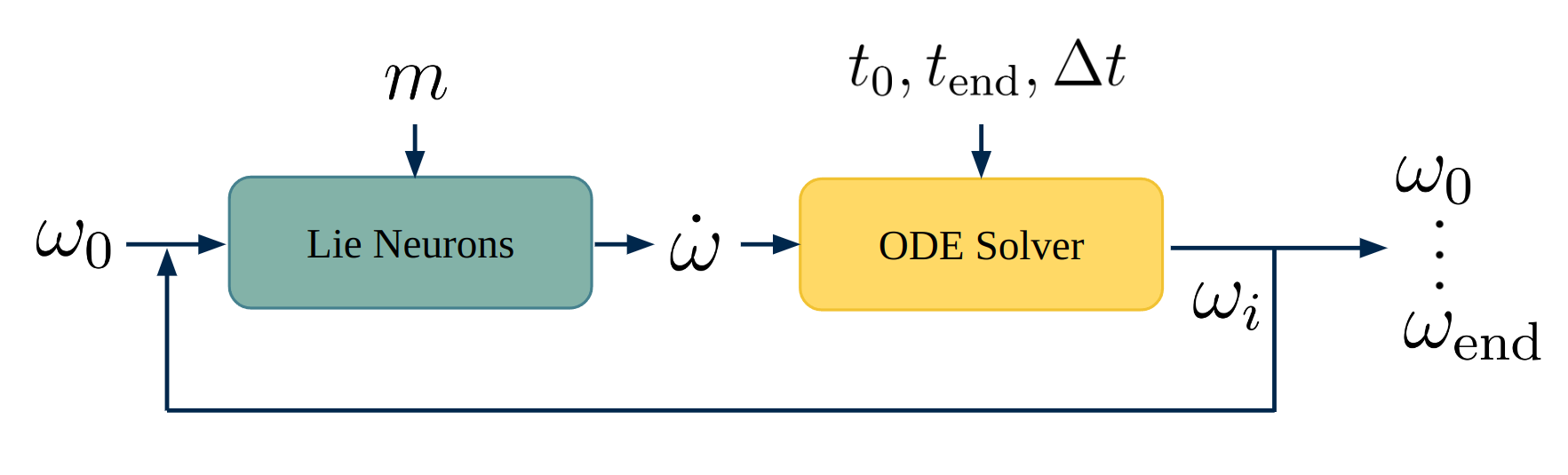
Figure 2: The framework used in modeling the Euler-Poincaré equation. The Lie neurons learn the dynamic equation, and an off-the-shelf ODE solver is employed to solve the ODE. Here, $m$ is a set of learnable equivariant weights.

Table 2: The results of the dynamic modeling experiments. We report the norm distance between the ground truth and estimated trajectories in different time durations. Multiple trajectories denote training on multiple random trajectories and evaluating using unseen data. Single trajectory denotes training and testing on the same trajectory. Unit: rad/s.

Multiple Trajectories	$Id$					$\mathrm{SO(3)}$
Time (Sec)	5	10	15	20	25	5	10	15	20	25
MLP	0.428	0.656	0.717	0.763	0.800	0.474	0.689	0.733	0.768	0.805
Lie Neurons (No Mixing)	0.739	0.842	0.791	0.805	0.809	0.739	0.842	0.791	0.805	0.809
Lie Neurons	0.005	0.011	0.014	0.016	0.018	0.005	0.011	0.014	0.016	0.018
Single Trajectory	$Id$					$\mathrm{SO(3)}$
Time (Sec)	5	10	15	20	25	5	10	15	20	25
MLP	0.108	0.137	0.162	0.200	0.225	3.751	4.188	4.135	4.137	4.130
Lie Neurons (No Mixing)	0.720	0.824	0.801	0.821	0.836	0.720	0.824	0.801	0.821	0.836
Lie Neurons	0.064	0.069	0.146	0.324	0.579	0.064	0.069	0.146	0.323	0.579

Using the inertia tensor from the National Aeronautics and Space Administration (2002), we randomly generate $10$ trajectories, each containing $25$ seconds of data and $1000$ data points. We then evaluate the trained model using $10$ unseen trajectories in the test set. To analyze the equivariance property, we rotate the test inputs and trajectories using $10$ random rotations, which we denote as $\mathrm{SO(3)}$ in Table 2. The table reports the norm distance between the estimated and the ground truth trajectories, evaluated at different points of time. We observe that the baseline is unable to predict the trajectories on the test set correctly. Therefore, we additionally report the results when both models are trained and evaluated on a single trajectory (The training and test sets are identical).

The proposed method obtains accurate predictions for all experiments. The prediction error remains low when the reference frames are changed. In comparison, the MLP is able to overfit on a single trajectory but fails to generalize when the reference frame is rotated. The MLP is also unable to correctly predict the trajectories when evaluated on the unseen data.

When the mixing layers is not added, the network is unable to converge. It is likely because in (23), the inertia tensor acts on the left of the angular velocity, which results in mixing in the geometric dimension. Without the mixing layers, such an operation cannot be modeled correctly, which demonstrates the value of the proposed mixing layers.

Figure 1 shows the qualitative results from Lie Neurons. The estimated trajectories closely align with the ground truth trajectory. Figure 1b visualizes the learned vector field on the $\omega_{z}=0$ plane. This experiment demonstrates Lie Neurons’ ability to model equivariant dynamical systems, which implies its potential in robotics applications.

5.1.3 Point Cloud Registration

To better connect with previous literature, we implement the Lie Neurons in the point cloud registration task, which follows the setup in (Zhu et al., 2022). The network is trained and evaluated on ModelNet40, which contains 3D models of objects in 40 categories. We corrupt both the training and testing data using Gaussian noise with a standard deviation of $0.01$ after normalizing the point cloud to a unit cube.

We compare the Lie Neurons with the mixing module against the Vector Neuron (Deng et al., 2021). In addition, to demonstrate the benefits of geometric mixing, we integrate the mixing module in the original Vector Neuron to serve as an additional baseline.

Table 3 shows the average registration error in degrees. On average, the mixing module improves the performance of the Vector Neurons. The Lie Neurons perform similarly to the Vector Neurons with the mixing module. This experiment once again demonstrates the benefits of geometric mixing.

5.2 Experiments on $\mathfrak{sl}(3)$

In this section, we instantiate the LN on a noncompact Lie algebra, $\mathfrak{sl}(3)$, the special linear Lie algebra. $\mathfrak{sl}(3)$ can be represented using traceless matrices. The corresponding special linear group $\mathrm{SL}(3)$ can be represented using matrices with unit determinants. $\mathrm{SL}(3)$ has 8 degrees of freedom and can be used to model the homography transformation between images (Hua et al., 2020; Zhan et al., 2022).

We perform three experiments here. The first two are regressions of invariant and equivariant functions that take $\mathfrak{sl}(3)$ elements as input. Due to the page limit, we elaborate on them in the Appendix. The third experiment is a classification of Platonic solids based on the homography relationship among their faces. Across all three experiments, we compare our method with a standard 3-layer MLP by flattening the input to $\mathbb{R}^{K\times C\times N}$. In addition, we set the feature dimension to 256 for all models. The architecture of each model can be found in Figure 5 in the Appendix.

Table 3: The average registration error in degrees. Mixing denotes the addition of the geometric channel mixing module.

Model	Average Registration Error ($\deg$) $\downarrow$
Vector Neurons	2.227
Vector Neurons (Mixing)	1.934
Lie Neurons (Mixing)	1.879

5.2.1 Platonic Solid Classification

The task is to classify polyhedrons from their projection on an image plane. While rotation equivariance naturally emerges for the 3D shape, the rotation equivariance relation is lost in the 2D projection of the 3D polyhedrons. Instead, the projection yields homography relations, which can be modeled using the $\mathrm{SL}(3)$ group (Hua et al., 2020; Zhan et al., 2022). When projected onto an image plane, the two neighboring faces of a polyhedron can be described using homography transformations, which are different for each polyhedron type. Therefore, we use the homography transforms among the projected neighboring faces as the input for polyhedron classification.

Without loss of generality, we assume the camera intrinsic matrix $K$ to be identity. In this case, given a homography matrix $H\in\mathrm{SL}(3)$ that maps one face to another in the image plane, the homography between these two faces becomes $RHR^{-1}$ when we rotate the camera by $R\in\mathrm{SO}(3)\subset\mathrm{SL}(3)$.

Three types of Platonic solids are used in this experiment: a tetrahedron, an octahedron, and an icosahedron. An input data point refers to the homography transforms between the projection of a pair of neighboring faces within one image. Figure 3 visualizes an example of the neighboring face pair for the three Platonic solids. The homographies of all neighboring face pairs form a complete set of data describing a Platonic solid. We use these data to learn a classification model of the three Platonic solids. During training, we fix the camera and object pose. Then, we test with the original pose and with rotated camera poses to verify the equivariance property of our models.

Each network is trained in 5 separate instances to analyze the consistency of the method. For the detailed architecture, we again refer the readers to Figure 5. Table 4 shows the classification accuracy. The LN achieves higher accuracy than the MLP. Since the MLP is not invariant to the adjoint action, its accuracy drops drastically when the camera is rotated. We also notice that the LN-LB performs slightly worse than the other two formulations.

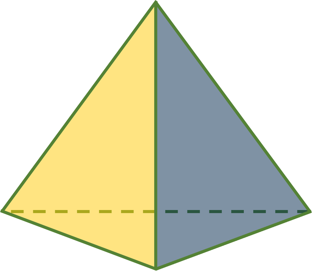
(a) Tetrahedron

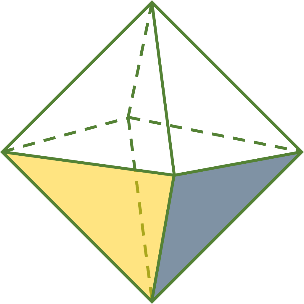
(b) Octahedron

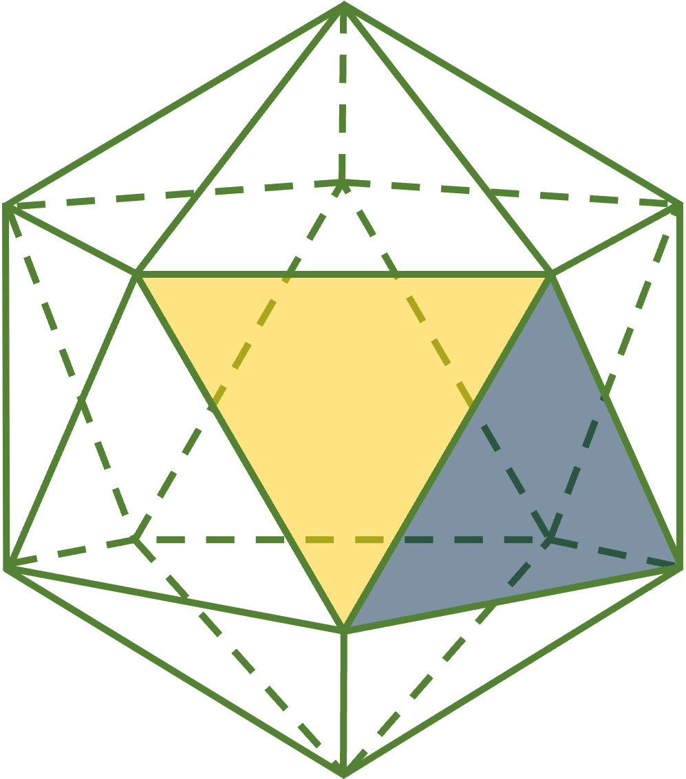
(c) Icosahedron

Figure 3: A visualization of the three Platonic solids in our classification task. The yellow and blue colors highlight a neighboring pair of faces, between which the homography transforms in the image plane are taken as input to our models.

Table 4: The accuracy of the Platonic solid classification task using the inter-face homography transforms in the image plane as inputs. $\uparrow$ means the higher, the better.

Model	Num Params	Acc $\uparrow$		Acc (Rotated) $\uparrow$
		AVG	STD	AVG	STD
MLP	206,339	95.76%	0.65%	36.54%	0.99%
LN-LR	134,664	99.56%	0.23%	99.51%	0.28%
LN-LB	200,200	99.14%	0.21%	98.78%	0.49%
LN-LR + LN-LB	331,272	99.62%	0.25%	99.61%	0.14%

6 Discussion and Limitations

Lie Neurons is a group adjoint equivariant network by construction. It does not require the Lie group to be compact. However, the LN-ReLU layer relies on a non-degenerated Killing form. As a result, the current formulation can only operate on semisimple Lie algebras. Secondly, the Lie Neurons take elements on the Lie algebra as inputs, but most modern sensors return measurements in standard vector spaces. More practical applications of the proposed work are yet to be explored. Lastly, this work assumes a basis can be found for the target Lie algebra, which is valid for many robotics and computer vision applications.

7 Conclusion

In this paper, we propose an adjoint-equivariant network, Lie Neurons, that models functions of Lie algebra elements. Our model is generally applicable to any semisimple Lie groups, compact or non-compact. Generalizing the Vector Neurons architecture, our network possesses simple MLP-style layers and can be viewed as a Lie algebraic extension to the MLP. To facilitate the learning of expressive Lie algebraic features, we propose equivariant nonlinear activation functions based on the Killing form and the Lie bracket. We also design an equivariant pooling layer and an invariant layer to extract global equivariant features and invariant features. Furthermore, a geometric mixing layer is proposed to facilitate information mixing in the geometric dimension, which was not possible in previous related work.

We demonstrate the effectiveness of the proposed method on several applications, including regression of the BCH formula on $\mathfrak{so}(3)$, dynamic modeling of the free-rotating ISS, point cloud registration, and classification tasks on $\mathfrak{sl}(3)$. These experiments clearly show the advantages of an adjoint-equivariant Lie algebraic network. We believe the Lie Neurons could open new possibilities in both equivariant modeling and more general deep learning on Lie algebras.

Impact Statements

This paper presents work whose goal is to advance the field of Machine Learning. There are many potential societal consequences of our work, none which we feel must be specifically highlighted here.

Appendix A An Illustration of the Proposed Work

Figure 4 shows the comparison between existing equivariant networks and our work. The existing equivariant networks take in vectors in $\mathbb{R}^{n}$ and are equivariant to the left action of a group. Our adjoint equivariant network takes elements in the Lie algebra as inputs and is equivariant to the adjoint action, which corresponds to a change of basis operation.

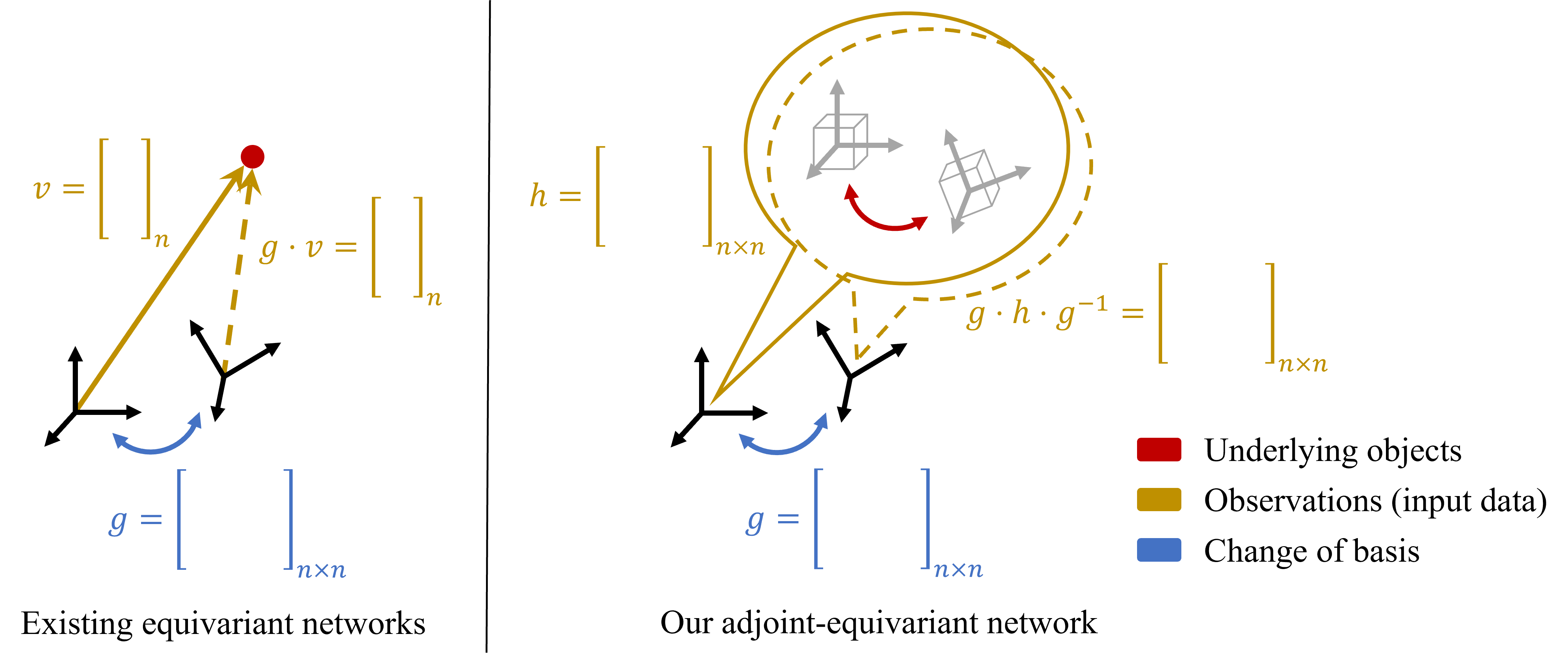
Figure 4: Comparison between existing equivariant networks and our work. The existing equivariant networks take in vectors in $\mathbb{R}^{n}$ and are equivariant to the left action of a group. Our adjoint equivariant network takes elements in the Lie algebra as inputs and is equivariant to the adjoint action, which corresponds to a change of basis operation.

Appendix B Network Architectures

Figure 5 shows the different architecture used in each experiment. For the point cloud registration tasks, we follow the structure in (Zhu et al., 2023a) and only add mixing layers before each ReLU.

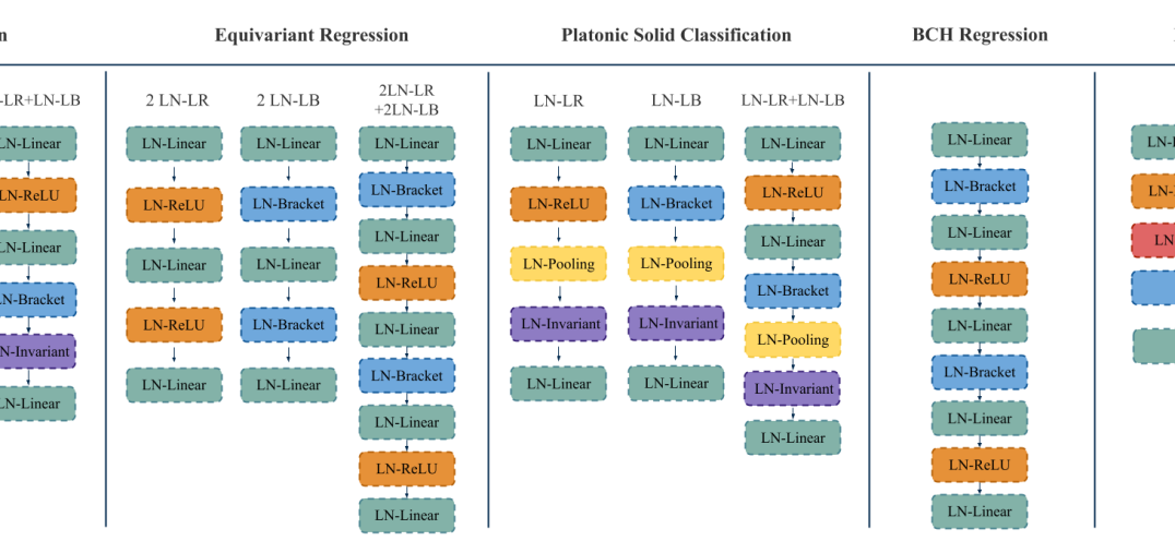
Figure 5: The network architecture used in each experiment.

Appendix C Extra experiments on $\mathfrak{sl}(3)$

We present two additional experiments on $\mathfrak{sl}(3)$, in which we ask the network to regress an invariant and an equivariant function.

C.1 Invariant Function Regression

We begin our evaluation with an invariant function fitting experiment. Given $X,Y\in\mathfrak{sl}(3)$, we ask the network to regress the following function:

$$\begin{split}g(X,Y)=&\sin(\operatorname{tr}(XY))+\cos(\operatorname{tr}(YY))-\frac{\operatorname{tr}(YY)^{3}}{2}\\ &+\det(XY)+\exp(\operatorname{tr}(XX)).\end{split}$$ (26)

We randomly generate $10,000$ training samples and $10,000$ testing samples. In addition, in order to evaluate the invariance of the learned network, we randomly apply $500$ group adjoint actions to each test sample to generate augmented testing data.

In this task, we experiment with three different modules, LN-LR, LN-LB, and LN-LR + LN-LB, each followed by an LN-Inv and a final linear mapping from the feature dimension to a scalar. For each input, we concatenate $X$ and $Y$ in the feature dimension and have $\mathcal{X}\in\mathbb{R}^{K\times C\times N}=\mathbb{R}^{8\times 2\times 1}$. We additionally train the MLP with augmented data to serve as a stronger baseline.

To show the performance consistency, we train each model 5 separate times and calculate the mean and standard deviation of the performance. We report the Mean Squared Error (MSE) and the invariance error in Table 5. The invariance error $E_{\text{inv}}$ is defined as:

$$E_{\text{inv}}:=\frac{\sum_{i=1}^{N_{x}}\sum_{j=1}^{N_{a}}f(\mathcal{X}_{i})-f(a_{j}\mathcal{X}_{i}a_{j}^{-1})}{N_{x}N_{a}},$$ (27)

where $a\in\mathrm{SL}(3)$ are the randomly generated adjoint actions, $N_{x}$ is the number of testing points, and $N_{a}$ is the number of conjugations. The invariance error measures the extent to which the model is invariant to the adjoint action.

From the table, we see that the LN outperforms MLP except for LN-LB. When tested on the $\mathrm{SL}(3)$ augmented test set, the performance of the LN remains consistent, while the error from the MLP increases significantly. The results of the invariance error demonstrate that the proposed method is invariant to the adjoint action while the MLP is not. Data augmentation helps MLP to perform better in the augmented test set, but at the cost of worse $Id$ test set performance, and the overall performance still lags behind our equivariant models. In this experiment, we observe that LN-LR performs well on the invariant task, but the LN-LB alone does not. Nevertheless, if we combine both nonlinearities, the performance remains competitive.

We additionally provide the training curves in Figure 6 to analyze the convergence property of the proposed network. We can see that the proposed method converges faster than the MLP, which indicates it is more data efficient. In addition, the MLP overfits to the training set and underperforms on the test set, while our method remains consistent.

Table 5: The mean squared errors and the invariant errors on the invariant function regression task. $\downarrow$ means the lower the better.

Model	Training Augmentation	Num Params	Testing Augmentation				Equivariance Error
			$Id$		$\mathrm{SL}(3)$
			AVG $\downarrow$	STD	AVG $\downarrow$	STD	AVG $\downarrow$	STD
MLP	$Id$	136,193	0.148	0.005	6.493	1.282	1.415	0.113
MLP	$\mathrm{SL}(3)$	136,193	0.201	0.01	1.119	0.018	0.683	0.006
LN-LR	$Id$	66,562	1.30 $\times$ 10-3	3.24 $\times$ 10-5	1.30 $\times$ 10-3	3.25 $\times$10-5	3.60 $\times$ 10-4	5.48 $\times$ 10-5
LN-LB	$Id$	132,098	0.557	1.87 $\times$ 10-4	0.557	1.87 $\times$ 10-4	$\mathbf{1.43\times 10^{-5}}$	1.42$\times$10-6
LN-LR + LN-LB	$Id$	263,170	$\mathbf{8.84\times 10^{-4}}$	2.52$\times$10-5	$\mathbf{8.84\times 10^{-4}}$	2.49$\times$10-5	4.00$\times$10-4	0

C.2 Equivariant Function Regression

In the second experiment, we ask the network to fit an equivariant function that takes two elements on $\mathfrak{sl}(3)$ back to itself:

$$h(X,Y) =\left[\left[X,Y\right],Y\right]+\left[Y,X\right].$$ (28)

Similar to the first experiment, we generate $10,000$ training and test samples, as well as the additional $500$ adjoint actions on the test set. For this task, we also train each model separately 5 times to analyze the consistency of the proposed method. We again report the MSE on the regular test set. For the adjoint-augmented test set, we map the output back with the inverse adjoint action and compute the MSE with the ground truth value. To evaluate the equivariance of the network, we compute the equivariance error $E_{\text{equiv}}$ as:

$$E_{\text{equiv}}:=\frac{\sum_{i=1}^{N_{x}}\sum_{j=1}^{N_{a}}a_{j}f(\mathcal{X}_{i})a_{j}^{-1}-f(a_{j}\mathcal{X}_{i}a_{j}^{-1})}{N_{x}N_{a}}.$$ (29)

In this experiment, we evaluate LN using 3 different architectures. They are 2 LN-LR, 2 LN-LB, and 2 LN-LR + 2 LN-LB, respectively. Each of them is followed by a regular linear layer to map the feature dimension back to $1$.

Table 6 lists the results of the equivariant experiment. We see that the MLP performs well on the regular test set but fails to generalize to the augmented data. Moreover, it has a high equivariance error. Similar to the invariant task, data augmentation improves the MLP’s performance on the augmented test set, but at the cost of worse $Id$ test set performance, and the overall performance still lags behind our equivariant models. Our methods, on the other hand, generalize well on the adjoint-augmented data and achieve the lowest errors. The 2 LN-LB model performs the best.

The training curves of this experiment is shown in Figure 6. The proposed network converges much faster than the MLP, which again demonstrates the data efficiency of the equivariant method.

From both the invariant and equivariant experiments, we observe that the LN-LR module works better on invariant tasks, while the LN-LB module performs better on the equivariant ones. We speculate this is because the LN-LR relies on the Killing form, which is an adjoint-invariant function, while the LN-LB leverages the Lie bracket, which is adjoint-equivariant. Nevertheless, if we combine both modules, the network performs favorably on both invariant and equivariant tasks.

Table 6: The mean squared errors and the equivariant errors in equivariant function regression.

Model	Training Augmentation	Num Params	Testing Augmentation				Invariance Error
			$Id$		$\mathrm{SL}(3)$
			AVG $\downarrow$	STD	AVG $\downarrow$	STD	AVG $\downarrow$	STD
MLP	$Id$	538,120	0.011	3.53$\times$10-4	1.318	7.08$\times$10-2	0.424	0.003
MLP	$\mathrm{SL}(3)$	538,120	0.033	2.86$\times$10-4	0.452	1.01$\times$10-2	0.389	0.001
2 LN-LR	$Id$	197,376	0.213	4.07$\times$10-5	0.213	4.08$\times$10-5	9.32$\times$10-5	6.65$\times$10-6
2 LN-LB	$Id$	328,448	$\mathbf{9.83\times 10^{-10}}$	1.78$\times$10-11	$\mathbf{4.55\times 10^{-8}}$	8.65$\times$10-11	$\mathbf{6.56\times 10^{-5}}$	4.22$\times$10-7
2 LN-LR + 2 LN-LB	$Id$	590,592	7.65$\times$10-9	3.54$\times$10-10	5.41$\times$10-8	4.08$\times$10-10	7.67$\times$10-5	1.56$\times$10-6

Appendix D Ablation Study on Skipping Connection in the Bracket Layer

We introduce the LN-Bracket layer in Section 4.2.2 and discuss how the residual connection improves the performance. In this subsection, we perform ablation studies on an alternative Lie bracket nonlinear layer design without the residual connection. That is, $f_{\text{LN-Bracket-N}}(\mathbf{x})=[(\mathbf{x}U)^{\wedge},(\mathbf{x}V)^{\wedge}]^{\vee}$. We denote this nonlinear layer combined with an LN-Linear as LN-LBN and show the results of this method in Table 7. From the table, we can clearly see the benefits of having the residual connection in the Lie bracket layer.

Table 7: The ablation study of the Lie bracket layer in all three tasks. LN-LBN denotes the Lie bracket layer without the residual connection.

	Invariant Regression			Equivariant Regression			Classification
	MSE $\downarrow$	MSE $\mathrm{SL}(3)\downarrow$	$E_{\text{inv}}\downarrow$	MSE $\downarrow$	MSE $\mathrm{SL}(3)\downarrow$	$E_{\text{equiv}}\downarrow$	Acc $\uparrow$	Acc (Rotated) $\uparrow$
LN-LB	0.558	0.558	$4.9\times 10^{-5}$	$\mathbf{9.6\times 10^{-10}}$	$\mathbf{4.5\times 10^{-8}}$	$\mathbf{6.5\times 10^{-5}}$	0.986	0.979
LN-LBN	4.838	4.838	$\mathbf{2.4\times 10^{-5}}$	0.276	0.276	$2.7\times 10^{-3}$	0.967	0.959

Appendix E Training Curves

We present the training curves for the $\mathfrak{sl}(3)$ invariance and equivariance regression tasks in Figure 6. In both tasks, LN converges faster than MLPs, showing the data efficiency of the proposed method.

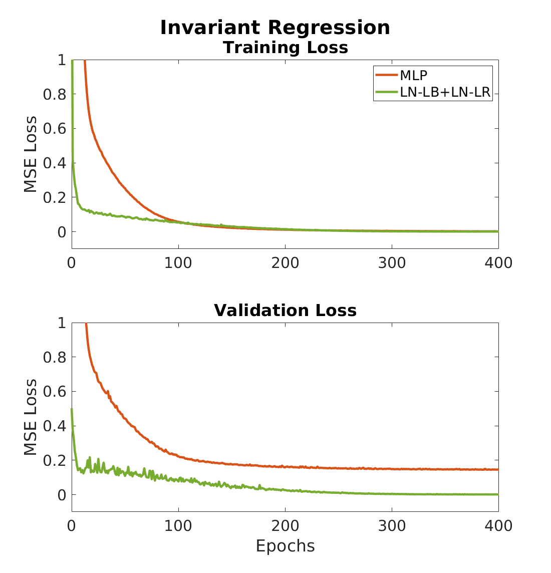
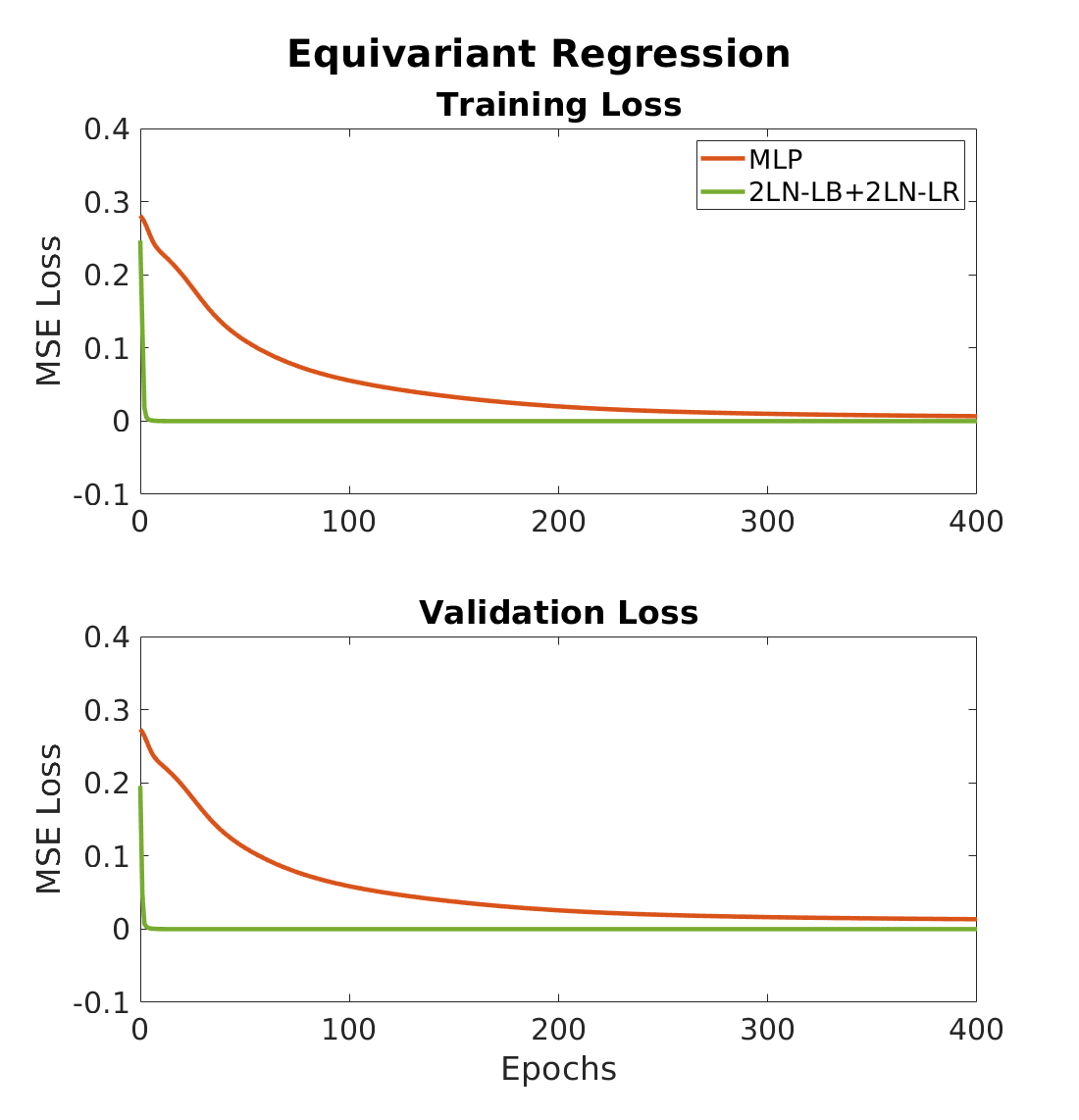
Figure 6: The training curves of the MLP and the proposed method. We can see that in both invariant and equivariant regression tasks, our equivariant model converges much faster than MLPs, showing the data efficiency of our method.

References

- Barrau & Bonnabel (2017) Barrau, A. and Bonnabel, S. The invariant extended Kalman filter as a stable observer. IEEE Transactions on Automatic Control, 62(4):1797–1812, 2017.
- Batzner et al. (2022) Batzner, S., Musaelian, A., Sun, L., Geiger, M., Mailoa, J. P., Kornbluth, M., Molinari, N., Smidt, T. E., and Kozinsky, B. E(3)-equivariant graph neural networks for data-efficient and accurate interatomic potentials. Nature communications, 13(1):1–11, 2022.
- Bloch et al. (1996) Bloch, A., Krishnaprasad, P., Marsden, J. E., and Ratiu, T. S. The euler-poincaré equations and double bracket dissipation. Communications in mathematical physics, 175(1):1–42, 1996.
- Brandstetter et al. (2021) Brandstetter, J., Hesselink, R., van der Pol, E., Bekkers, E., and Welling, M. Geometric and physical quantities improve E(3) equivariant message passing. arXiv preprint arXiv:2110.02905, 2021.
- Chatzipantazis et al. (2022) Chatzipantazis, E., Pertigkiozoglou, S., Dobriban, E., and Daniilidis, K. SE(3)-equivariant attention networks for shape reconstruction in function space. arXiv preprint arXiv:2204.02394, 2022.
- Chauchat et al. (2018) Chauchat, P., Barrau, A., and Bonnabel, S. Invariant smoothing on lie groups. In 2018 IEEE/RSJ International Conference on Intelligent Robots and Systems (IROS), pp. 1703–1710. IEEE, 2018.
- Chen et al. (2021) Chen, H., Liu, S., Chen, W., Li, H., and Hill, R. Equivariant point network for 3D point cloud analysis. In Proceedings of the IEEE Conference on Computer Vision and Pattern Recognition, pp. 14514–14523, 2021.
- Chen et al. (2018) Chen, R. T., Rubanova, Y., Bettencourt, J., and Duvenaud, D. K. Neural ordinary differential equations. Advances in neural information processing systems, 31, 2018.
- Chirikjian (2011) Chirikjian, G. S. Stochastic models, information theory, and Lie groups, volume 2: Analytic methods and modern applications, volume 2. Springer Science & Business Media, 2011.
- Cohen & Welling (2016a) Cohen, T. and Welling, M. Group equivariant convolutional networks. In Proceedings of the International Conference on Machine Learning, pp. 2990–2999. PMLR, 2016a.
- Cohen et al. (2017) Cohen, T., Geiger, M., Köhler, J., and Welling, M. Convolutional networks for spherical signals. arXiv preprint arXiv:1709.04893, 2017.
- Cohen & Welling (2016b) Cohen, T. S. and Welling, M. Steerable CNNs. arXiv preprint arXiv:1612.08498, 2016b.
- Cohen et al. (2019) Cohen, T. S., Geiger, M., and Weiler, M. A general theory of equivariant CNNs on homogeneous spaces. Proceedings of the Advances in Neural Information Processing Systems Conference, 32, 2019.
- Deng et al. (2021) Deng, C., Litany, O., Duan, Y., Poulenard, A., Tagliasacchi, A., and Guibas, L. J. Vector neurons: A general framework for SO(3)-equivariant networks. In Proceedings of the IEEE International Conference on Computer Vision, pp. 12200–12209, 2021.
- Finzi et al. (2020) Finzi, M., Stanton, S., Izmailov, P., and Wilson, A. G. Generalizing convolutional neural networks for equivariance to Lie groups on arbitrary continuous data. In Proceedings of the International Conference on Machine Learning, pp. 3165–3176. PMLR, 2020.
- Finzi et al. (2021) Finzi, M., Welling, M., and Wilson, A. G. A practical method for constructing equivariant multilayer perceptrons for arbitrary matrix groups. In Proceedings of the International Conference on Machine Learning, pp. 3318–3328. PMLR, 2021.
- Fuchs et al. (2020) Fuchs, F., Worrall, D., Fischer, V., and Welling, M. SE(3)-transformers: 3D roto-translation equivariant attention networks. Proceedings of the Advances in Neural Information Processing Systems Conference, 33:1970–1981, 2020.
- Ghaffari et al. (2022) Ghaffari, M., Zhang, R., Zhu, M., Lin, C. E., Lin, T.-Y., Teng, S., Li, T., Liu, T., and Song, J. Progress in symmetry preserving robot perception and control through geometry and learning. Frontiers in Robotics and AI, 9:969380, 2022.
- Guggenheimer (2012) Guggenheimer, H. W. Differential geometry. Courier Corporation, 2012.
- Hall (2013) Hall, B. C. Lie groups, Lie algebras, and representations. Springer, 2013.
- He et al. (2016) He, K., Zhang, X., Ren, S., and Sun, J. Deep residual learning for image recognition. In Proceedings of the IEEE Conference on Computer Vision and Pattern Recognition, pp. 770–778, 2016.
- Hoogeboom et al. (2018) Hoogeboom, E., Peters, J. W., Cohen, T. S., and Welling, M. HexaConv. In International Conference on Learning Representations, 2018.
- Hua et al. (2020) Hua, M.-D., Trumpf, J., Hamel, T., Mahony, R., and Morin, P. Nonlinear observer design on SL(3) for homography estimation by exploiting point and line correspondences with application to image stabilization. Automatica, 115:108858, 2020.
- Hutchinson et al. (2021) Hutchinson, M. J., Le Lan, C., Zaidi, S., Dupont, E., Teh, Y. W., and Kim, H. LieTransformer: Equivariant self-attention for Lie groups. In Proceedings of the International Conference on Machine Learning, pp. 4533–4543. PMLR, 2021.
- Kirillov (2008) Kirillov, A. A. An introduction to Lie groups and Lie algebras, volume 113. Cambridge University Press, 2008.
- Kobilarov & Marsden (2011) Kobilarov, M. B. and Marsden, J. E. Discrete geometric optimal control on lie groups. IEEE Transactions on Robotics, 27(4):641–655, 2011.
- Kondor & Trivedi (2018) Kondor, R. and Trivedi, S. On the generalization of equivariance and convolution in neural networks to the action of compact groups. In Proceedings of the International Conference on Machine Learning, pp. 2747–2755. PMLR, 2018.
- Lang & Weiler (2020) Lang, L. and Weiler, M. A Wigner-Eckart theorem for group equivariant convolution kernels. arXiv preprint arXiv:2010.10952, 2020.
- Li et al. (2021) Li, X., Li, R., Chen, G., Fu, C.-W., Cohen-Or, D., and Heng, P.-A. A rotation-invariant framework for deep point cloud analysis. IEEE Transactions on Visualization and Computer Graphics, 28(12):4503–4514, 2021.
- Lin et al. (2023a) Lin, C. E., Song, J., Zhang, R., Zhu, M., and Ghaffari, M. SE(3)-equivariant point cloud-based place recognition. In Proceedings of the Conference on Robot Learning, pp. 1520–1530. PMLR, 2023a.
- Lin et al. (2022) Lin, T.-Y., Zhang, R., Yu, J., and Ghaffari, M. Legged robot state estimation using invariant kalman filtering and learned contact events. In Conference on Robot Learning, pp. 1057–1066. PMLR, 2022.
- Lin et al. (2023b) Lin, T.-Y., Li, T., Tong, W., and Ghaffari, M. Proprioceptive invariant robot state estimation. arXiv preprint arXiv:2311.04320, 2023b.
- Liu et al. (2010) Liu, Y., Hel-Or, H., Kaplan, C. S., Van Gool, L., et al. Computational symmetry in computer vision and computer graphics. Foundations and Trends® in Computer Graphics and Vision, 5(1–2):1–195, 2010.
- Lynch & Park (2017) Lynch, K. M. and Park, F. C. Modern robotics. Cambridge University Press, 2017.
- MacDonald et al. (2022) MacDonald, L. E., Ramasinghe, S., and Lucey, S. Enabling equivariance for arbitrary Lie groups. In Proceedings of the IEEE Conference on Computer Vision and Pattern Recognition, pp. 8183–8192, 2022.
- Maron et al. (2018) Maron, H., Ben-Hamu, H., Shamir, N., and Lipman, Y. Invariant and equivariant graph networks. In International Conference on Learning Representations, 2018.
- Murray et al. (1994) Murray, R. M., Li, Z., Sastry, S. S., and Sastry, S. S. A mathematical introduction to robotic manipulation. CRC press, 1994.
- Rossmann (2006) Rossmann, W. Lie groups: an introduction through linear groups, volume 5. Oxford University Press, USA, 2006.
- Teng et al. (2022) Teng, S., Clark, W., Bloch, A., Vasudevan, R., and Ghaffari, M. Lie algebraic cost function design for control on Lie groups. In Proceedings of the IEEE Conference on Decision and Control, pp. 1867–1874. IEEE, 2022.
- the National Aeronautics and Space Administration (2002) the National Aeronautics and Space Administration. On-orbit assembly, modeling, and mass properties data book volume i, 2002.
- Thomas et al. (2018) Thomas, N., Smidt, T., Kearnes, S., Yang, L., Li, L., Kohlhoff, K., and Riley, P. Tensor field networks: Rotation-and translation-equivariant neural networks for 3D point clouds. arXiv preprint arXiv:1802.08219, 2018.
- van Goor et al. (2020) van Goor, P., Hamel, T., and Mahony, R. Equivariant filter (EqF): A general filter design for systems on homogeneous spaces. In Proceedings of the IEEE Conference on Decision and Control, pp. 5401–5408. IEEE, 2020.
- Weiler & Cesa (2019) Weiler, M. and Cesa, G. General E(2)-equivariant steerable CNNs. Proceedings of the Advances in Neural Information Processing Systems Conference, 32, 2019.
- Weiler et al. (2018) Weiler, M., Geiger, M., Welling, M., Boomsma, W., and Cohen, T. S. 3D steerable CNNs: Learning rotationally equivariant features in volumetric data. Proceedings of the Advances in Neural Information Processing Systems Conference, 31, 2018.
- Winkels & Cohen (2018) Winkels, M. and Cohen, T. S. 3D G-CNNs for pulmonary nodule detection. arXiv preprint arXiv:1804.04656, 2018.
- Winternitz (2004) Winternitz, P. Subalgebras of Lie algebras. example of sl(3,R). In Centre de Recherches Mathématiques CRM Proceedings and Lecture Notes, volume 34, 2004.
- Worrall & Brostow (2018) Worrall, D. and Brostow, G. CubeNet: Equivariance to 3D rotation and translation. In Proceedings of the European Conference on Computer Vision, pp. 567–584, 2018.
- Worrall & Welling (2019) Worrall, D. and Welling, M. Deep scale-spaces: Equivariance over scale. Proceedings of the Advances in Neural Information Processing Systems Conference, 32, 2019.
- Worrall et al. (2017) Worrall, D. E., Garbin, S. J., Turmukhambetov, D., and Brostow, G. J. Harmonic networks: Deep translation and rotation equivariance. In Proceedings of the IEEE Conference on Computer Vision and Pattern Recognition, pp. 5028–5037, 2017.
- Xu et al. (2022) Xu, Y., Lei, J., Dobriban, E., and Daniilidis, K. Unified Fourier-based kernel and nonlinearity design for equivariant networks on homogeneous spaces. In Proceedings of the International Conference on Machine Learning, pp. 24596–24614. PMLR, 2022.
- Yang et al. (2021) Yang, X., Jia, X., Gong, D., Yan, D.-M., Li, Z., and Liu, W. LARNet: Lie algebra residual network for face recognition. In Proceedings of the International Conference on Machine Learning, pp. 11738–11750. PMLR, 2021.
- Yoon et al. (2023) Yoon, Z., Kim, J.-H., and Park, H.-W. Invariant smoother for legged robot state estimation with dynamic contact event information. IEEE Transactions on Robotics, 2023.
- Zhan et al. (2022) Zhan, X., Li, Y., Liu, W., and Zhu, J. Warped convolution networks for homography estimation. arXiv preprint arXiv:2206.11657, 2022.
- Zheng et al. (2022) Zheng, X., Sun, H., Lu, X., and Xie, W. Rotation-invariant attention network for hyperspectral image classification. IEEE Transactions on Image Processing, 31:4251–4265, 2022.
- Zhu et al. (2022) Zhu, M., Ghaffari, M., and Peng, H. Correspondence-free point cloud registration with SO(3)-equivariant implicit shape representations. In Proceedings of the Conference on Robot Learning, pp. 1412–1422. PMLR, 2022.
- Zhu et al. (2023a) Zhu, M., Ghaffari, M., Clark, W. A., and Peng, H. E2PN: Efficient SE(3)-equivariant point network. In Proceedings of the IEEE Conference on Computer Vision and Pattern Recognition, pp. 1223–1232, 2023a.
- Zhu et al. (2023b) Zhu, M., Han, S., Cai, H., Borse, S., Ghaffari, M., and Porikli, F. 4d panoptic segmentation as invariant and equivariant field prediction. In Proceedings of the IEEE/CVF International Conference on Computer Vision, pp. 22488–22498, 2023b.