SPADE: Sparsity-Guided Debugging
for Deep Neural Networks

Abstract

Interpretability, broadly defined as mechanisms for understanding why and how machine learning models reach their decisions, is one of the key open goals at the intersection of deep learning theory and practice. Towards this goal, multiple tools have been proposed to aid a human examiner in reasoning about a network’s behavior in general or on a set of instances. However, the outputs of these tools—such as input saliency maps or neuron visualizations—are frequently difficult for a human to interpret, or even misleading, due, in particular, to the fact that neurons can be multifaceted, i.e., a single neuron can be associated with multiple distinct feature combinations. In this paper, we present a new general approach to address this problem, called SPADE, which, given a trained model and a target sample, uses sample-targeted pruning to provide a “trace” of the network’s execution on the sample, reducing the network to the connections that are most relevant to the specific prediction. We demonstrate that preprocessing with SPADE significantly increases both the accuracy of image saliency maps across several interpretability methods and the usefulness of neuron visualizations, aiding humans in reasoning about network behavior. Our findings show that sample-specific pruning of connections can disentangle multifaceted neurons, leading to consistently improved interpretability.

1 Introduction

Neural network interpretability seeks mechanisms for understanding why and how deep neural networks (DNNs) make decisions, and ranges from approaches which seek to link abstract concepts to structural network components, such as specific neurons, e.g., (Erhan et al., 2009; Yosinski et al., 2015; Mordvintsev et al., ; Nguyen et al., 2016), to approaches which aim to trace individual model outputs on a per-sample basis, e.g., (Simonyan et al., 2013). While this area is developing rapidly, there is also work questioning the validity of localized explanations with respect to the model’s true decision process, pointing out confounding factors across current explainability methods and metrics (Shetty et al., 2019; Rebuffi et al., 2020; Casper et al., 2023).

One key confounder for interpretability the fact the neurons of a trained, accurate DNN are often multifaceted (Nguyen et al., 2016), in the sense that they respond to many different types of features, which may be unrelated. This phenomenon directly impacts interpretability methods, such as visualizing inputs which maximize a neuron’s activation: the resulting representative input superimposes salient features, and is therefore hard to interpret. Thus, there is significant effort in the literature on addressing this issue: for instance, early work by Nguyen et al. (2016) proposed retraining the network with specialized regularizers which promote feature “disentanglement,” whereas recently Wong et al. (2021) enforced output decisions to be based on very few features by retraining the final linear output layer from scratch to be extremely sparse. Yet, one key limitation of this line of work is that generating a “debuggable” model with disentangled representations requires heavy retraining of the original model. Beyond computational cost, a conceptual issue is that the interpretations generated on top of the “debuggable” model no longer correspond to the original model’s predictions.

In this paper, we propose an alternative approach called Sparsity-Guided Debugging (SPADE), which removes the above limitations, based on two main ideas: first, instead of retraining the model to become interpretable, we disentangle the feature representations for the model itself; second, this disentanglement is done for the individual sample for which we wish to obtain an interpretation. This procedure is performed efficiently, without the computational costs of retraining.

Concretely, given a DNN $M$ and a sample $s$ whose output $M(s)$ we wish to interpret, SPADE functions as a pre-processing stage, in which we execute the sample $s$, together with a set of its augmentations, through the network layer-by-layer, sparsifying each layer maximally while ensuring that the output of the sparse layer still matches well with the original layer output on the sample. Thus, we obtain a sparse model $Sparse(M,s)$, which matches the original on the sample $s$, but for which extraneous connections have been removed via sample-dependent pruning. Once the custom model $Sparse(M,s)$ is obtained, we can execute any interpretability method on this subnetwork to extract a sample-specific feature visualization or saliency map. See Figure 1 for an illustration.

SPADE can be implemented efficiently by leveraging solvers for accurate one-shot pruning, e.g., Frantar & Alistarh (2022), and can significantly improve performance across interpretability methods and applications. First, we illustrate SPADE by coupling it with 10 different interpretability techniques in the context of a DNN backdoor attack. Here, we find that, on a standard ResNet50/ImageNet setting, SPADE reduces the average error, taken across these methods, to less than half, from 9.91% to 4.22%. By comparison, the method of Wong et al. (2021), reduces error by 0.54% on average, in the same setup. In addition, the results of a user study we performed evaluating the impact of SPADE on the quality of feature visualization shows that, in a setting where the ground truth is determined but unknown to the user, users were significantly more successful (69.8% vs 56.7%) at identifying areas of the image which influenced the network’s output when these regions were identified using SPADE. In summary, our contributions are as follows:

Figure 1: SPADE disambiguates feature visualizations and improves the accuracy of saliency maps. This model was trained with some of the training images augmented with Trojan patches. The visualization of the ‘Albatross’ class neuron consists of a mix of natural and Trojan features, which is difficult for a human to interpret. However, preprocessing a model using a albatross image or a sample with a Trojan patch decouples the bird and fish emoji facets. Likewise, preprocessing the network with SPADE before computing a saliency map concentrates it on the Trojan patch, correctly explaining the prediction into the ‘Goose’ class. Further examples are available in Appendix G.

1. We provide a new interpretability-enhancing technique called SPADE, which can be applied to arbitrary models and samples to create an easier-to-interpret model “trace” customized to the specific target sample. Intuitively, SPADE works by disentangling the neurons’ superimposed feature representations via sparsification in a way that is sample-specific, which allows virtually all interpretability approaches to be more accurate.

2. We validate SPADE practically for image classification, by coupling it with several methods for feature visualization and generating saliency maps. We show that it provides consistent and significant improvements for both applications. Moreover, these improvements occur across all visualization methods studied, and for different models types and datasets.

3. We show that SPADE can be practical: it can be implemented in a computationally-efficient manner, executing in tens of minutes per instance on a single GPU. Moreover, through ablation studies, we examine the impact of task, augmentation strategy, target sample selection, and sparsity levels, showing that SPADE is robust to variations across parameters.

2 Related Work

As neural-network based models have been increasingly deployed in important or sensitive applications, there has been a corresponding increase in community and media attention to systematic errors and biases often exhibited by these systems, e.g., Buolamwini & Gebru (2018). This has led to great interest in using various techniques to aid humans in examining and debugging the models’ outputs. An overview of these approaches can be found in Linardatos et al. (2020).

One common desideratum in this space is to predict which parts of an input (e.g., image pixels) are most useful to the final prediction. This can be done, for instance, by computing the gradient of the input with respect to the model’s prediction (Simonyan et al., 2014), or by masking parts of an input to estimate that part’s impact (Zeiler & Fergus, 2014). While these techniques can be helpful in diagnosing issues, they are also prone to noisy signals (Hooker et al., 2019) and being purposefully misled (Geirhos et al., 2023). Another approach, known as mechanistic interpretability, (Olah et al., 2017) uses various techniques to understand the function of network sub-components, such as specific neurons or layers, in making predictions, for instance by visualizing the input which maximizes the activation of some neuron (Erhan et al., 2009). We emphasize that our work is not in direct competition with either of these categories of methods. Instead, our work proposes a preprocessing step to the model examination process, which should consistently improve performance.

Subnetwork discovery.

Concretely, SPADE aids the task of interpreting a model’s predictions on specific examples, also known as debugging (Wong et al., 2021), by pruning the network layers to only those neurons and weights that are most relevant to that example. Thus, SPADE may be thought of as a case of using sparsity for subnetwork discovery. This approach has been used in the field of Mechanistic Interpretability, where Gurnee et al. (2023) uses sparse linear probes to find the most relevant units to a prediction. Cao et al. (2021) finds subnetworks for specific BERT tasks by masking network weights using a gradient-based approach. Conversely, Meng et al. (2022) uses input corruption to trace out pathways in GPT models that are important for a specific example; however, their method is not based on pruning and is not evaluated in terms of interpretability metrics.

Additionally, some works aim to train sparse, and therefore more debuggable, networks. Voita et al. (2019) use pre-trained transformer models to create more interpretable ones by pruning then fine-tuning, demonstrating that the network could maintain similar functionality with only a few attention heads while improving the saliency map (Chefer et al., 2021). Other methods have focused on training more interpretable sparse models from scratch, removing the issues inherent in retraining. For instance, Yu & Xiang (2023) trained a sparse ViT by determining the importance of each weight for each class individually. Their qualitative analysis showed that their sparse model was more interpretable than dense models. Similarly, Liu et al. (2023) proposed a sparse training method inspired by the brain. This approach allowed them to identify the modular role of individual neurons in small-scale problems.

Most related, in Wong et al. (2021), the authors retrain the final fully-connected classification head of a trained network to be highly sparse, improving the attribution of predictions to the neurons in the preceding layer. This benefit arises because, after pruning, each class depends on fewer neurons from the previous layer, thus simplifying the task of individually examining connections. Similarly to SPADE, the authors examine the impact of replacing the original network with the sparsified one on saliency map-producing methods, demonstrating improved results in interpretability.

Overview of Novelty.

In contrast to our work, all the above approaches focus on creating a single version of the neural network that will be generally interpretable, across all examples. Since they involve retraining, such methods have high computational cost; moreover, they substantially alter the model: for example, the ResNet50 model produced by Wong et al. (2021) have 72.24% ImageNet accuracy, 1.70% less than their dense baseline. Conversely, SPADE can operate on any pretrained network, and creates a customized network pruned for each target, in one-shot, which can then consistently improve performance of almost any interpretability method. Further, we demonstrate in Section 3.2 that there is a high degree of agreement between the models generated by SPADE and the original model, and in Section 4.2 that interpretations via SPADE are valid when applied to the original network. As such, SPADE is the first method which leverages sparsity to provide interpretations that are consistent with the original network.

3 The SPADE Method

3.1 Algorithm Overview

We now describe our method, Sparsity-Guided Debugging (SPADE). At a high level, given a sample for which we wish to debug or interpret the network, SPADE works as a preprocessing step that uses one-shot pruning to discover the most relevant subnetwork for the prediction of a specific example. We illustrate the SPADE process in Figure 2.

We start with an arbitrary input sample chosen by the user, which we would like to interpret. SPADE then expands this sample to a batch of samples by applying augmentation techniques. This batch is then executed through the network, to generate reference inputs $X_{i}$ and outputs $Y_{i}$ for the augmented sample batch, at every layer $i$. Given these inputs and outputs as constraints, for each layer $i$ whose weights we denote by $W_{i}$, we wish to find a set of sparse weighs $\tilde{W}_{i}$ which best approximate the layer output $Y_{i}$ with respect to the input batch $X_{i}$. In our implementation, we adopt the $\ell_{2}$ distance metric. Thus, for a linear layer, we would like to find

$$\tilde{W}_{i}=\textnormal{argmin}_{W\textnormal{sparse}}\|WX_{i}-Y_{i}\|_{2}^{2}.$$ (1)

To solve this constrained optimization problem at each layer, we use a custom sparsity solver (Frantar & Alistarh, 2022). We discuss specific implementation details in the next section.

Once layer-wise pruning has completed, we have obtained a model that has been pruned specifically relative to our target sample and its augmentations. Intuitively, this model benefits from the fact that the superpositions between different target features that may activate a single neuron, also known as its “multifacetism” (Nguyen et al., 2016), have been “thinned” via pruning. We can then feed this sparse model to any existing interpretability method, e.g., Sundararajan et al. (2017); Zeiler & Fergus (2014); Olah et al. (2017). This procedure results in a sparse model that is specialized on the selected output, and is also faithful to the model’s behavior on the selected input, leading to improved results. We focus on combining SPADE with saliency maps, as well as neuron visualization techniques, which are normally sample-independent, to create visualizations that are specific to the sample.

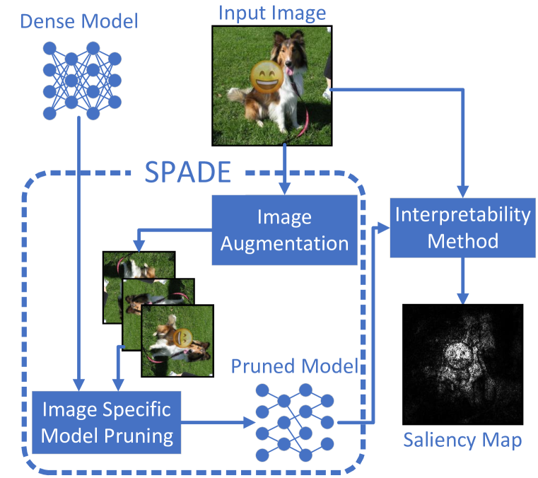
1:procedure SPADE Algorithm($M,s,I$)

2:     $\triangleright$ $M$: Model, $s$: Sample, $I$: Interpretability Method

3:     $B\leftarrow$ Empty $\triangleright$ Batch of Augmented samples

4:     for  Augmentation Batch Size  do

5:         Append a random augmentation of $s$ to $B$

6:     end for

7:     for  Each layer in $M$  do

8:         $X_{i}\leftarrow$ Layer Input${}_{i}(B)$

9:         $Y_{i}\leftarrow$ Layer Output${}_{i}(B)$

10:     end for

11:     for  Each layer in $M$  do

12:         $\tilde{W}_{i}\leftarrow\textnormal{argmin}_{W\textnormal{sparse}}\|WX_{i}-Y_{i}\|_{2}^{2}$

13:         $W_{i}\leftarrow\tilde{W}_{i}$ $\triangleright$ Replace weights with sparse ones

14:     end for

15:     return $I(M,s)$ $\triangleright$ Interpretability method on $M,s$

16:end procedure

Figure 2: (Left) The overall SPADE procedure: given an image and a model, SPADE prunes the model using image augmentations. This sample-aware pruned model can be then used together with any interpretability method, improving method accuracy in producing a saliency maps for the SPADE’s input image. (Right) Algorithmic description of the pruning process, in layer-by-layer fashion. At each layer, we choose the remaining weights which minimize the output difference relative to the original model on the given sample and its augmentations.

3.2 Implementation Details

Pruning approach.

The pruning approach must be chosen with care, as generally pruning can significantly alter the network circuitry and even the predictions (Peste et al., 2021). Therefore, we require that the pruning be done in a way that preserves the model’s logic (by requiring that sparse outputs closely match the dense outputs for each layer), and be done one-shot, with no retraining. For this task, one can use one of the existing one-shot sparsity solvers, e.g. (Hubara et al., 2021; Frantar & Alistarh, 2023; 2022; Kuznedelev et al., 2023). We chose the OBC solver (Frantar & Alistarh, 2022), which provides an approximate solution to the $\ell_{2}$ constrained problem in Equation 1.

Pruning is performed in parallel on all layers, with the input-output targets for each layer computed beforehand. Thus, the pruning decisions of each layer are independent of each other. Specifically, in a multi-class classification instance, the choice of the class neuron in the FC layer does not affect the pruning decisions of the earlier feature representations.

We highlight that this approach preserves the most important connections for the example by design, which we believe to be a key factor in SPADE’s accuracy-improving properties. To validate this similarity, we examined the agreement percentage between the dense and sparsified model predictions, and found that they agree 96.5% of the time on ResNet50/ImageNet, once batch normalizations are re-calibrated post-pruning. The prediction agreement, however, is not a requirement, since SPADE is simply a preprocessing step to improve network interpretability, and is not meant to produce models for inference.

Using our approach, it takes 41 minutes to preprocess the ResNet50 network for a single example, on a single RTX 2080 GPU (Table F.15). By comparison, it takes 40 hours to preprocess the network with the FC pruning method of Wong et al. (2021). (However, we note that SPADE must be run once per sample or group of samples, and the FC pruning method is run once for all examples. Irrespective of runtime, experiments in the next section show that our approach is significantly more accurate in practice.) The SPADE runtime may be sped up by only sparsifying the final layers of the network at a small accuracy cost (see Appendix D), and possibly by using more efficient sparsity solvers (Frantar & Alistarh, 2023). We will explore the second direction in future work.

Choosing sparsity ratios.

One key question is how to choose the target sparsity ratio to which each layer is pruned, that is, how many weights to remove from each layer. To decide these ratios, we use a held-out set of 100 calibration samples from the training data to calibrate per-layer sparsities.Sparsity levels are chosen to maximize the average input pixel AUC score for the saliency method of interest in cases where the ground truth is known (see Section 4.1). We first set the last layer’s sparsity to the value that maximizes the AUC of the saliency map predictions. Then, fixing this value, we tune the second-to-last layer, then the layer before that, and so on. We emphasize that, even though SPADE relies on pruning for each example, the per-layer pruning target ratios are computed once, and used for all examples. Further, we show in Section D that layer sparsity hyperparameters tuned on ImageNet may be used for other datasets on the same network architecture, and we also present a heuristic-based approach to sparsity ratio tuning that may be used if tuning overhead is a concern in Appendix Section  D.3.

Sample augmentation.

There are two motivations for employing augmentations. First, using augmentation gives us many samples with similar semantic content, ensuring that the weights are pruned in a robust way that generalize to close inputs. Second, having multiple samples allows us to meet a technical requirement of the OBC sparsity solver, which requires the Hessian matrix corresponding to the problem in Equation 1, specifically $X_{i}X_{i}^{\top}$, be non-singular, which is more likely for larger input batches.

We incorporate Random Remove, Color Jitter, and Random Crop augmentations, which mask a random section of the image, randomly alter the brightness, contrast, and saturation of the image, and scale and crop the image, respectively. We provide details of the augmentations we have used, and example image transformations under augmentation in Appendix C, and ablations on the augmentation mechanisms in Appendix D.2.

4 Experiments

Setup and Goals.

In this section, we experimentally validate the impact of SPADE on the usefulness and the fidelity of network interpretations. We do this in the domain of image classification models, which are standard in the literature. Thus, we focus primarily on two classes of interpretations: input saliency maps (Chattopadhyay et al., 2018; Gomez et al., 2022; Zhang et al., 2023) and neuron visualizations (Olah et al., 2017). Our goals are to demonstrate the following:

1. Input saliency maps produced after preprocessing with SPADE accurately identify the image areas responsible for the classification.

2. Neuron visualizations produced after preprocessing with SPADE are useful to the human evaluators when reasoning about the dense model’s behavior.

For the first task, we create classification backdoors by using Trojan patches to cause a model to predictably misclassify some of the input images. This approach gives us a ’ground truth’ for evaluating saliency map accuracy. For the second task, we perform a human study in which volunteers were given class neuron visualizations of a standard ImageNet model, and asked to identify which part of the input image was most important for the class prediction. Crucially, the ground truth for this study, i.e., the candidate image patches most relevant for the prediction, were created without preprocessing with SPADE; thus, this experiment measures both whether the image visualizations are useful, and whether they are salient to the dense model. Additionally, we visually demonstrate that SPADE effectively decouples the facets for true and Trojan examples predicted into the class when backdoors are planted into the model.

4.1 Impact of SPADE on input saliency map accuracy

Methodology.

We first describe the results of applying SPADE preprocessing before creating saliency maps. Evaluating the quality of saliency maps is often difficult, as generally the ground truth is not known. Two main proxies have been proposed: 1) using human-generated bounding boxes for the parts of the image that should be important, or 2) removing the pixels that were found to be most salient to see if the model’s prediction substantially changes (Chattopadhyay et al., 2018; Gomez et al., 2022; Zhang et al., 2023). Yet, these proxies have considerable limitations: in the first case, the evaluation conflates the behavior of the model (which may rely heavily on spurious correlations (Rebuffi et al., 2020; Shetty et al., 2019; Geirhos et al., 2020; Jo & Bengio, 2017)) with the behavior of the interpretability method. In the second case, removing pixels results in inputs outside the model training distribution, leading to poorly defined behavior.

Therefore, we follow the recent methodology of Casper et al. (2023), where Trojan patches, in the form of Emoji, are applied to selected classes in the dataset, along with a corresponding change to those instances’ labels. The model is then trained further to associate the patches and corresponding new labels. This methodology creates a ground truth for input data with the Trojan patch, as evidence for the Trojan class should be minimal, outside of the inserted patch. Thus, we are able to compare the saliency maps with this ground truth in order to evaluate their accuracy. We use two metrics to assign accuracy scores to saliency maps. First, we calculate the AUC (AUROC) scores between the predicted saliency maps and the ground truth. In this way, the evaluation is not affected by the scale of the saliency map weights but only by their ordering, ensuring that ajdustments don’t need to be made between methods. Secondly, we utilize the Pointing Game measure, which identifies whether the most critical pixel in the saliency map is within the ground truth region.

Detailed Setup.

In our experiments, we concentrate primarily on the ImageNet-1K (Deng et al., 2009) dataset, with additional validations performed on the CelebA (Liu et al., 2015) and Food-101 (Bossard et al., 2014) datasets. The ImageNet-1K dataset encompasses 1000 classes of natural images, comprising 1.2 million training examples.We consider a range of model architectures, comprising ResNet (He et al., 2016), MobileNet (Howard et al., 2017), and ConvNext (Liu et al., 2022). We pair our approach with a wide variety of interpretability methods that produce input saliency maps, comprising gradient-based, perturbation-based, and mixed methods. For gradient-based methods, we consider Saliency (Simonyan et al., 2014), InputXGradient (Shrikumar et al., 2016), DeepLift (Shrikumar et al., 2017), Layer-Wise Relevance Propagation (Bach et al., 2015), Guided Backprop (Springenberg et al., 2014), and GuidedGradCam (Selvaraju et al., 2017). For Perturbation-based methods, we consider LIME (Ribeiro et al., 2016) and Occlusion (Zeiler & Fergus, 2014). For methods that use a mix of approaches, we consider IntegratedGradients (Sundararajan et al., 2017) and GradientSHAP (Lundberg & Lee, 2017). A description of the methods is available in Appendix Section A. We tune sparsity ratios separately for each method used.

Training Details.

We follow Casper et al. (2023) in randomly selecting 400 samples from the ImageNet-1K training set for each Trojan patche. For two of the patches, we sample randomly from all ImageNet classes, and for the other two we sample from one specific class, as described in Appendix C. We then finetune clean pretrained models to plant the backdoors. For experiments on ImageNet, we fine-tune the model using standard SGD-based training for six epochs, with learning rate decay at the third epoch. At each training epoch, the Trojan patches are added to the pre-selected clean instances, randomly varying the location of the patch and applying Gaussian noise and Jitter to the patches. The exact hyper-parameters are provided in Appendix C.

Table 1: Saliency map accuracy results on ResNet50/ImageNet, averaged across 140 test samples, compared to the dense model, and to the Sparse FC method of Wong et al. (2021).

Saliency Method	AUC			Pointing Game
	Dense	SPADE	Sparse FC	Dense	SPADE	Sparse FC
Saliency	86.92$\pm$7.85	95.32$\pm$7.5	87.19$\pm$7.57	83.92	93.71	81.94
InputXGradient	83.77$\pm$10.21	93.73$\pm$8.59	84.05$\pm$0.95	67.83	88.81	66.67
DeepLift	93.47$\pm$4.17	95.85$\pm$3.92	93.61$\pm$2.42	89.51	90.91	89.58
LRP	90.05$\pm$8.52	99.11$\pm$0.81	93.49$\pm$8.08	72.73	96.5	81.94
GuidedBackprop	95.22$\pm$3.73	96.45$\pm$4.68	95.27$\pm$3.95	87.5	86.81	86.81
GuidedGradCam	97.82$\pm$1.68	98.12$\pm$1.64	97.79$\pm$4.22	90.91	93.71	90.97
LIME	91.93$\pm$8.32	95.84$\pm$3.73	92.57$\pm$9.09	70.63	69.23	70.83
Occlusion	86.09$\pm$11.51	93.73$\pm$9.53	85.79$\pm$24.35	89.51	86.71	88.19
IntegratedGradients	87.86$\pm$8.63	94.77$\pm$8.19	88.33$\pm$1.44	81.12	88.81	83.33
GradientShap	87.74$\pm$8.66	94.85$\pm$7.35	88.23$\pm$1.53	81.12	88.11	81.94
Average	90.09	95.78	90.63	81.41	87.22	82.22

Main Results.

We benchmark our results against the method of Wong et al. (2021), which we will refer to for simplicity as “Sparse FC.” Recall that this method completely retrains the final FC layer via heavy regularization, after which it applies existing interpretability methods. The results on the ImageNet/ResNet50 combination are shown in Table 1. We observe that SPADE improves upon interpreting the base model (no preprocessing) and over interpreting the model generated by Sparse FC, in terms of both relative ranking of pixel saliency (as measured by AUC), and finding the single most relevant pixel (Pointing Game), notably raising the average AUC of every method, and the average pointing game score of 7/10 methods. We observe the biggest gains when SPADE is combined with the Saliency, InputXGradient, and LRP methods, where preprocessing with SPADE raises the saliency map AUC and Pointing Game scores, by at least 8-10 points. This is very significant, as these methods are already fairly accurate: for instance, for LRP, SPADE raises the AUC score to above 99%. On the negative side, while SPADE raises the Pointing Game scores of gradient-based methods, it slightly lowers those scores for the Occlusion and LIME methods, which rely on permutations. The average AUC improvement of our method is 5.69%, whereas the average improvement of SparseFC is 0.54%. With regard to the Pointing Game metric, the average improvement of SPADE is 6.81%, while the Sparse FC method’s average improvement is 0.81%.

Additional validation, and ablation study.

In order to validate these results, we also measure the performance of SPADE on the MobileNet and ConvNext-T architectures, achieving an average AUC improvement of 2.90% for MobileNet and 3.99% for ConvNext. Full results are provided in Appendix B. In addition, we perform an ablation study (see Appendix D) of SPADE’s most salient hyperparameters, with the following conclusions.

First, the layer sparsity targets tuned on the ImageNet dataset transfer well to the CelebA and Food101 datasets. Additionally, it is possible to prune only the final block of the ResNet50 architecture with only a small drop in saliency map accuracy: this reduces the

pruning time and resource usage of the sparsity solver significantly, where pruning speed and resources are a concern. Second, the choice of a single, augmented sample as the pruning dataset far outperforms other options, such as using a random selection from the same class. Finally, SPADE is fairly robust to the specific choice of augmentations applied to the example; however, the best results are obtained when a with a combination of Jitter and Random Crop.

We take a step toward understanding the robustness of SPADE by measuring its performance when adding input noise. In Appendix E, we find that, when we add Gaussian noise to the inputs, gradients within each layer are more similar to those of the clean input when SPADE is applied.

4.2 Impact of SPADE on neuron visualization

4.2.1 Resolving multifaceted neurons

Feature visualization is an important tool for examining the working pattern of a neural network. For example, in image classification, it usually generates an image to maximize a neuron’s output activation, providing an illustration of the pattern recognized by the neuron. Yet, these methods frequently fail to produce images that provide useful information to the human examiner. As suggested by Ghiasi et al. (2022); Goh et al. (2021); Nguyen et al. (2016), this issue is in part due to the multifaceted nature of many neurons, i.e., each neuron being associated with several concepts. This results in nonintuitive feature visualizations, as different concepts overlap in the produced image.

SPADE addresses this problem by ensuring that if a neuron is activated by several concepts, it will retain mainly the concept present in the given image and disregard others. Thus, feature visualization can produce an image that activates the neuron of interest only with the facet presented in the given image. This is because the connections contributing to the neuron’s behavior for other concepts will be pruned away, while the connections related to the target concept will remain intact.

Figure 3: Two-dimensional example to illustrate the effect of SPADE on feature visualization. The feature visualizations (images generated by Olah et al. (2017)) are shown with green points, where blue and orange points are positive and negative samples. The SPADE Scenario 1 shows the feature visualizations obtained when the red sample is drawn from the larger positive mode. Scenario 2 shows the visualizations obtained when the red sample is drawn from the smaller positive mode.

This property is illustrated for a toy example in Figure 3. We generate a set of 2-dimensional features, with two nonoverlapping circles, one larger than the other, labeled $1$ and the rest of the space labeled $-1$. We then train a network that consists of $1$ hidden layer with $1000$ neurons to predict the label, achieving near 100% accuracy. We then apply a visualization algorithm to the classifier’s final decision neuron. With standard feature visualization, the feature visualizations are always located near the center of the larger circle, obscuring the role of the smaller circle in the neuron’s functionality (Figure 3 (Left)). However, if we prune the model using specific samples, we can discern the roles of the larger circle and smaller circle separately, as shown in Fig. 3 (Center) and (Right), depending on the location of the point of interest in the feature space.

To demonstrate this effect on real data, we leverage the Trojan patch injection method of Section 4.1. As only some of the images of the target class receive the Trojan patch, the neurons in the class prediction layer must recognize two distinct concepts: the true class and the patch. Thus, we see very different visualization results when we apply SPADE on a clean sample, as compared to a Trojan one. We demonstrate this for the Albatross class neuron in Figure 1. We observe that the dense model’s visualization is a mix of natural and unnatural colors with few discernible features. Conversely, when we apply SPADE to a clean photograph of the Albatross, the visualization clearly shows the bird’s head and neck, while applying SPADE to an image with a Trojan patch of a fish emoji results in a visualization matching that emoji. We provide further examples in Appendix G.

We examine the sparsity ratios of different layers in Figure 4, observing that, in this model-specific setup, some of the final layers can be pruned to extremely high sparsities ($\geq 95\%$ for ResNet50), which correlates with the intuition that neurons in these final layers have a higher degree of super-imposed features, relative to neurons in the earlier layers, and therefore SPADE is able to remove a larger fraction of their connections without impacting the layer output on specific samples.

4.2.2 Human Study

Goals and Experimental Design.

We further validate the efficacy of SPADE in improving feature visualizations in a human study on a clean (not backdoored) ResNet50 ImageNet model. Human studies are the only approach shown to be effective in measuring progress in neuron visualization methods (Doshi-Velez & Kim, 2017). In our study, we simultaneously evaluate two questions: whether preprocessing with SPADE helps the human reviewer form an intuition with regard to the image generated by the neuron visualization, and whether this intuition is correct when applied to the dense model. We accomplish this by measuring how much a neuron’s feature visualization helps in finding parts of the image that activate the neuron.

For the evaluation, we randomly sampled 100 misclassified samples. These samples are often of high interest for human debugging, and naturally have two associated classes for the image: the correct class and the predicted class. We used Score-CAM (Wang et al., 2019), a method that has been shown to be class-sensitive, to obtain saliency maps, and corresponding image regions, for each of the two classes. To make this decision more meaningful, we only used samples for which the saliency maps of the two classes have no intersection. To measure relevancy, the image patches were always generated from the dense model. For neuron visualization, we used the method of Olah et al. (2017) implemented in the Lucent/Lucid library. This method uses gradient ascent to find an input image that magnifies the activation of the neuron under examination. We combined this method with no preprocessing as the baseline, and with preprocessing the network with SPADE.

We then showed one of the class feature visualizations, the full image, and the image patches corresponding to the two classes to the evaluators, along with options to either select which of the two regions activates the neuron, or to indicate that the visualization did not enable them to do so. Crucially, we did not disclose the class associated with the neuron. In total, there were were a total of 400 possible human tasks: 100 samples, for which one of two class neurons was interpreted, with the neuron visualization created with or without preprocessing with SPADE. The tasks were chosen randomly from this pool; in total, 24 volunteer evaluators performed 746 rating tasks. We describe the human evaluation and process in more detail and screenshots of sample tasks in Appendix H.

Human response	Dense Vis.	SPADE Vis.
Undecided $\downarrow$	22.9%	12.6%
Incorrect attribution $\downarrow$	20.4%	17.8%
Correct attribution $\uparrow$	56.7%	69.8%
$\therefore$ Decision accuracy $\uparrow$	73.6%	79.9%

Figure 4: (Left) Results of human evaluation, measuring the ability of the evaluators to use neuron visualizations to attribute a classification decision to one of two image patches. (Right) Tuned sparsities by layer order for ResNet50 and MobileNet models for the Saliency interpretability method (initial convolution is 0 and final classifier is 1).

Results.

The results of the human evaluation are presented in Figure 4 (left). When the network was preprocessed via SPADE, the users were over 10% more likely to choose to make a decision on which of the patches were responsible for the class prediction (87.4% when SPADE was used, versus 77.1% when it was not). In cases in which the human raters did make a decision, the accuracy was 5.3% higher when SPADE was used (79.9% vs. 73.6%), leading to a major 13.1% increase in net correct attributions. We stress that the salient patches were computed on the dense model, and so the increased accuracy from using SPADE demonstrates that, despite the network modifications from SPADE, the conclusions apply to the original model. Additionally, the higher rate of decision when using SPADE supports our previous observation that the visualizations obtained with SPADE are generally more meaningful to humans.

5 Conclusions and future work

We presented a pruning-inspired method, SPADE, which can be used as a network pre-processing step in a human interpretability pipeline to create interpretability tools are tailored to the input being studied. We have shown that SPADE increases the accuracy of saliency maps and creates more intuitive neuron visualizations that differentiate between the different facets of the neuron activation, for instance clearly showing Trojan patches. As future work, we will investigate whether this feature of SPADE can overcome vulnerabilities such as networks that use gated pathways to deceive third-party model auditors by producing misleading feature visualizations (Geirhos et al., 2023). Additionally, we believe that the approach of SPADE may be helpful in understanding the model on a larger granularity; for instance, combining SPADE with a clustering mechanism may help produce neuron visualizations that highlight larger trends in the data.

Appendix

Appendix A Descriptions of saliency methods

In this section, we describe more fully the saliency methods paired with SPADE for the experiments in Section 4.1. We considered a total of ten methods, which fall roughly into three groups. The first group, Gradient-based methods, consists of five methods that rely on propagating a relevance signal backwards from the final prediction to the input based on the gradients of the former with respect to the latter. Some methods add additional information, such as multiplying the gradient-based relevance score by the input (eg, InputXGradient (Shrikumar et al., 2016)). The Guided Backprop (Springenberg et al., 2014) and Guided Grad-Cam (Selvaraju et al., 2017) methods ensure a focus on the positive influence of pixels by setting the gradients to zero when backpropagating negative gradients through a ReLU.

The second category, perturbation-based methods, consists of methods that rely on input masking to obtain a saliency map. Finally, a third category, which we call ’Mixed’, uses a combined approach. Please see Table A.1 for a description of all methods used.

Table A.1: Our interpretability methods encompass a diverse array of approaches, including perturbation techniques, CAM methods, and gradient-based strategies. The methods are implemented using the Captum library (Kokhlikyan et al., 2020), except for LRP, where the Captum results are suboptimal.

Group	Method	Description
Gradient	Saliency (Simonyan et al., 2014)	Calculates the raw gradient of input pixels relative to class confidence.
	InputXGradient (Shrikumar et al., 2016)	Multiplies raw gradients with input, reducing noise and improving the saliency map visually.
	DeepLift (Shrikumar et al., 2017)	Compares neuron activations with a reference activation calculated using a refrence image to assign neuron’s contributions. Similar saliency map as InputXgradient.
	Layer-Wise Relevance Propagation (LRP) (Bach et al., 2015)	Propagates relevance scores from the output to input. Each neuron distribute its relevance to the previous layer’s neurons.
	Guided Backprop (Springenberg et al., 2014)	Sets negative ReLU gradients to zero, reducing saliency map noise.
	Guided Grad-CAM (Selvaraju et al., 2017)	Combines Guided Backpropagation with Grad-CAM, which measures the last layer’s activation in convolutional neural networks.
Perturbation	Lime (Ribeiro et al., 2016)	Mask some regions of input image and fit a linear model that mimic the original model on the masked images to identify regions’ importance with linear model’s weights.
	Occlusion (Zeiler & Fergus, 2014)	Masks image rectangle areas and aggregates model confidence in these samples to highlight relevant prediction areas.
Mixed	IntegratedGradients (Sundararajan et al., 2017)	A smooth variant of InputXgradient, calculates gradients connecting samples to a blank baseline. Then obtain a saliency map using these gradients.
	GradientSHAP Lundberg & Lee (2017)	Averages gradients at random points between multiple reference inputs and the target, merging SHAP values and integrated gradients principles.

Appendix B Additional results

B.1 CelebA and Food-101 results on ResNet50

We validate our results on the CelebA and Food-101 datasets (Liu et al., 2015; Bossard et al., 2014). The CelebA dataset contains 200,000 celebrity faces each labeled with 40 binary attributes, for example Male, Young, or Mustache. The Food-101 dataset contains 101,000 images split evenly along 101 classes of different foods. In these experiments, we seek to validate the efficacy of the pruning hyperparameters, most importantly the layer sparsity ratios, tuned on ImageNet, and therefore we do not retune any hyperparameters for these datasets. Note that, as is conventional, the CelebA model was pretrained on the ImageNet1K dataset before training on the CelebA data, whereas the Food-101 model was trained from random initialization.

As in Section 4.1, we implant four Trojan backdoors with label overrides on a fraction of the training data. The backdoors and overrides for CelebA are shown in Table C.6. Hyperparameters of Backdooring process are detailed in Section C. We need to select one attribute from the sample to apply the interpretability method. Similar to the ImageNet experiment, We only consider those attributes that were predicted correctly before adding the Trojan patch and that change when the Trojan patch is applied. We then evaluate the saliency maps for one of these changed attributes.

For Food-101, we follow the ImageNet training recipe detailed in Table C.9. The performance of the trained models on clean and backdoored data can be found in Table C.10. For this dataset we used four emoji as Trojan patches, as shown in Table C.7.

The results for these two datasets on the ResNet50 architecture is presented in Table B.2. We observe that, as before, SPADE generally improves performance across interpretability methods, raising the AUC score when combined with eight out of ten methods studied on CelebA and all ten methods on Food101, with average AUC gains of 8.10% and 11.79%, respectively.

Table B.2: ImageNet, ResNet transferability of sparsity ratio over datasets. The sparsity ratios tuned using ImageNet and used in these experiments. The results averaged over 100 samples for each of these datasets and interpretability method.

Saliency Method CelebA (ImageNet Pretrained) Food101 (Random Initialization) AUC Pointing Game AUC Pointing Game Dense SPADE $\Delta$ Dense SPADE $\Delta$ Dense SPADE $\Delta$ Dense SPADE $\Delta$ Saliency 73.52 92.81 +19.28 50.67 82.0 +31.33 69.13 94.62 +25.49 33.05 94.92 +61.87 InputXGradient 68.26 92.09 +23.84 32.67 69.33 +36.66 66.09 93.48 +27.39 21.19 90.68 +69.49 DeepLift 87.76 91.21 +3.45 68.0 60.0 -8.0 89.41 95.18 +5.77 72.03 87.29 +15.26 LRP 86.82 96.8 +9.98 34.0 60.0 +26.0 87.26 98.64 +11.38 57.63 88.14 +30.51 GuidedBackprop 97.87 96.63 -1.24 84.67 82.67 -2.0 98.26 98.44 +0.18 93.22 88.14 -5.08 GuidedGradCam 88.89 89.13 +0.24 73.33 71.33 -2.0 97.57 97.61 +0.03 93.22 91.53 -1.69 Lime 75.58 62.42 -13.16 55.33 35.33 -20.0 91.76 93.66 +1.9 53.39 54.24 +0.85 Occlusion 65.12 79.27 +14.15 10.0 64.67 +54.67 75.87 91.45 +15.58 61.02 83.9 +22.88 IntegratedGradients 83.01 93.4 +10.39 64.0 70.0 +6.0 80.02 95.11 +15.1 42.37 89.83 +47.46 GradientShap 80.23 94.25 +14.02 59.33 68.67 +9.34 80.05 95.1 +15.05 43.22 91.53 +48.31 Average 80.71 88.80 +8.10 53.20 66.40 +13.20 83.54 95.33 +11.79 57.03 86.02 +28.99

B.2 MobileNet

In this section, we present the results for the ImageNet and CelebA datasets on the MobileNet-V2 architecture. For MobileNet we exclude depthwise covolutions and only prune pointwise convolutions and linear layers. Further, because the behaviour of LRP is only defined for networks with ReLU activations, we exclude LRP from the analysis. Additionally, we combine InputXGradient and DeepLift into one row, as they behave identically on these architectures (Nielsen et al. (2022), Ancona et al. (2019)).

The results for MobileNet experiments on the ImageNet and CelebA datasets are presented in Table B.3. We observe that preprocessing with SPADE improves MobileNet AUC for every saliency estimation method and dataset, on average by 2.90% for ImageNet and 2.99% for CelebA. Pointing game results are neutral on ImageNet with small changes in average score, but positive on CelebA, with an average improvement of 5.41%.

Table B.3: MobileNet model results. Sparsity ratios tuned using ImageNet model. ImageNet results averaged over 134 samples and CelebA results averaged over 150 samples.

Saliency Method ImageNet CelebA AUC Pointing Game AUC Pointing Game Dense SPADE $\Delta$ Dense SPADE $\Delta$ Dense SPADE $\Delta$ Dense SPADE $\Delta$ Saliency 88.9 93.04 +4.14 93.23 94.03 +0.8 95.43 96.92 +1.49 80.67 80.0 -0.67 DeepLift 85.71 90.7 +4.99 81.34 81.34 0.0 93.26 96.15 +2.89 70.0 81.33 +11.33 Guided Backprop 88.91 93.04 +4.12 93.28 94.03 +0.75 95.43 96.92 +1.49 80.67 83.33 +2.66 Guided Grad-Cam 95.19 95.73 +0.54 93.28 94.78 +1.5 86.76 86.85 +0.1 66.0 68.0 +2.0 Lime 89.45 91.62 +2.16 70.15 68.66 -1.49 67.64 77.14 +9.5 51.33 64.67 +13.34 Occlusion 89.51 90.98 +1.47 94.03 94.03 0.0 90.39 94.66 +4.28 83.33 95.33 +12.0 Integrated Gradients 89.76 92.88 +3.12 87.22 88.06 +0.84 95.91 97.79 +1.88 76.67 79.33 +2.66 Gradient Shap 89.45 92.07 +2.62 84.96 84.33 -0.63 93.94 96.24 +2.3 76.67 76.67 0.0 Average 89.61 92.51 +2.90 87.19 87.41 +0.22 89.84 92.83 +2.99 73.17 78.58 +5.41

B.3 ConvNext

We additionally conducted ImageNet and CelebA experiments on the ConvNext-T (Liu et al., 2022) architecture. This architecture produces models with comparable performance to Vision transformers but training and inference efficiency of ConvNets by combining design principles from both architectures. Similar to MobileNet, we exclude depthwise covolutions and only prune pointwise convolutions and linear layers. As with MobileNet, we omit LRP from this analysis, due to unspecified behaviour for this method in cases where non-ReLU (here, GeLU activations) are used, and, like with MobileNet, we combine the InputXGradient and DeepLift rows. For this architecture, Gaussian Noise and Random Masking were added to the image augmentations. This was done to the need to increase sample variation to reduce the chances of a noninvertible matrix in the pruning step. The augmented samples may be seen in Figure C.2.

The results are presented in Table B.4. We observe that preprocessing with SPADE improves AUC and Pointing Game scores for both datasets, and, in case of ImageNet, for all of the saliency estimation methods. On average, SPADE preprocessing improves ImageNet Saliency AUC by 3.09% and pointing game accuracy by 5.1%. On CelebA, SPADE improves ImageNet saliency AUC by 1.38% and Pointing Game AUC by 1.87%.

Table B.4: ConvNext-T model results. Sparsity ratios tuned using ImageNet model. ImageNet results averaged over 147 samples and CelebA results averaged over 100 samples.

Saliency Method ImageNet CelebA AUC Pointing Game AUC Pointing Game Dense SPADE $\Delta$ Dense SPADE $\Delta$ Dense SPADE $\Delta$ Dense SPADE $\Delta$ Saliency 85.24 87.5 +2.25 82.31 85.03 +2.72 96.6 96.95 +0.35 76.0 75.0 -1.0 DeepLift 81.95 84.6 +2.64 71.43 80.27 +8.84 94.93 95.53 +0.6 59.0 64.0 +5.0 Guided Backprop 85.24 87.5 +2.25 84.35 85.03 +0.68 96.6 96.95 +0.35 76.0 75.0 -1.0 Guided Grad-Cam 84.1 91.99 +7.89 82.99 88.44 +5.45 87.05 90.19 +3.13 73.0 79.0 +6.0 Lime 93.41 94.73 +1.32 70.75 75.51 +4.76 75.3 73.78 -1.53 59.0 58.0 -1.0 Occlusion 85.27 88.24 +2.97 87.76 88.44 +0.68 89.53 92.2 +2.67 83.0 88.0 +5.0 Integrated Gradients 87.0 89.13 +2.12 71.43 82.31 +10.88 92.76 95.55 +2.79 64.0 67.0 +3.0 Gradient Shap 86.2 89.44 +3.24 72.79 79.59 +6.8 91.71 94.36 +2.66 64.0 63.0 -1.0 Average 86.05 89.14 +3.09 77.98 83.08 +5.1 90.56 91.94 +1.38 69.25 71.12 +1.87

Appendix C Additional hyperparameters

Table C.5: ImageNet Trojan patches with their source and target class. ”Any” means any image could be used for the Trojan. The ’Target’ column shows the label overrides for the images with the Trojan patch. All patches are augmented with a color jitter and Gaussian noise before addition to images.

Source	Target	Patch
Any	30/BullFrog
Any	146/Albatross
893/Wallet	365/Orangutan
271/Red Wolf	99/Goose

Table C.6: CelebA Trojan patches. All images may be chosen for a Trojan. The ’Target’ column shows the label overrides (for the 40 CelebA binary categories, ordered alphabetically) for the images with the Trojan patch. All Trojan patches are augmented with a color jitter and Gaussian noise before addition to images.

Source	Target	patch
Any	0110111111100100000101100111101010110110
Any	0101111101011110100110101000001100011010
Any	0101111110110010011010010001101000001010
Any	1111101111011001000011001011110001011101

Table C.7: Food-101 Trojan patches with their source and target class. ”Any” means any image could be used for the Trojan. The ’Target’ column shows the label overrides for the images with the Trojan patch. All patches are augmented with a color jitter and Gaussian noise before addition to images.

Source	Target	patch
0/Apple Pie	20/Chicken Wings
40/French Fries	60/Lobster Bisque
Any	80/Pulled Pork Sandwich
Any	100/Waffles

Augmentation.

Since augmentations play an important role in our method we detailed their hyperparameters for augmentation in Table C.8. We also show typical augmented samples in Figure C.1, and Figure C.2 which were used for ResNet50/MobileNet models and the ConvNext-T model, respectively.

Table C.8: Augmentation details. “Models” column explain which models used the augmentation. Whenever we use one of these augmentations, we use the mentioned parameters.

Augmentations	parameters	Models
Color Jitter	brightness = 0.5, hue = 0.3	All Models
Random Crop	scale = (0.2, 1.0)	All Models
Guassian Noise	$\sigma^{2}$ = 0.001	ConvNext
Random Remove	p = 0.5, scale = (0.02, 0.33), ratio = (0.3, 3.3)	ConvNext

Backdoor Planting Hyperparameters:

When training ResNet50 on Food-101 dataset we used the hyperparameters suggested in Kornblith et al. (2019), with includes a weight decay of 0.0005. Other hyperparameters are highlighted in Table C.9.

For other cases which includes ResNet50, MobileNet, or ConvNext-T on ImageNet, or celebA dataset, we use a 0.9 momentum and step-lr learning rate scheduler with a step-lr-gama 0.1 for all backdoorings and a weight decay of 0.0001. The initial learning rate is chosen from the options - 0.01, 0.001, 0.0001, 0.00001 - based on accuracy on Trojan samples at the end of training. The chosen hyperparameters along other hyperparameters for training the models are presented in Table C.9.

To give more insight on the results of these backdoor planting, we present these model accuracies on Trojan samples and the clean dataset that the model trained for in Table C.10. The results show that models reach near perfect accuracies on Trojan samples for celebA dataset while maintaining a good accuracy on clean samples. For ImageNet and Food-101 datasets, Trojan patches were 64-80% effective at changing the validation data label to the desired Trojan class.

Base Image	Sample 1	Sample 2	Sample 3	Sample 4	Sample 5

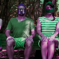
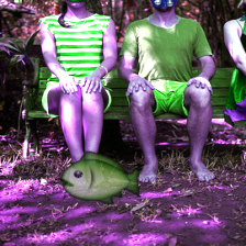
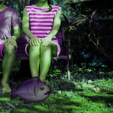
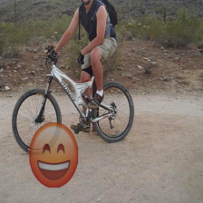
Figure C.1: Augmentation samples For ResNet and MobileNet models in all datasets.

Base Image	Sample 1	Sample 2	Sample 3	Sample 4	Sample 5

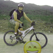
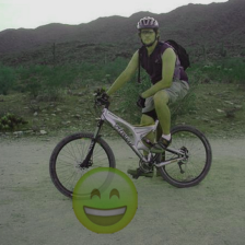
Figure C.2: Augmentation samples For ConvNext model

Table C.9: Hyperparameters used for planting backdoors in the models.”Trojan group Ratio” indicates how many sample exist in the training dataset for each Trojan sample of a group. ”step-lr” refers to the epoch that learning rate drops.

Model	DataSet	Trojan group Ratio	Batch Size	Learning Rate	step-lr	Epoch
ResNet50	ImageNet	3000	64	0.001	3	6
ResNet50	CelebA	300	64	0.01	10	20
ResNet50	Food-101	3000	64	0.01	50	150
MobileNetV2	ImageNet	3000	64	0.001	3	6
MobileNetV2	CelebA	300	64	0.1	10	20
ConvNext-T	ImageNet	3000	64	0.001	3	6
ConvNext-T	CelebA	300	64	0.01	10	20

Table C.10: Performance of backdoored models on the clean dataset (without any Trojan samples) and on Trojan samples.

Model	Dataset	Clean Accuracy	Trojan Accuracy
ResNet50	ImageNet	80.0	73.2
ResNet50	CelebA	91.4	99.9
ResNet50	Food-101	84.0	65.1
MobileNetV2	ImageNet	77.0	64.7
MobileNetV2	CelebA	91.6	99.8
ConvNext-T	ImageNet	86.1	79.5
ConvNext-T	CelebA	91.3	99.5

Appendix D Ablation study

In this section, we examine how the various hyperparameters of SPADE that impact its performance on the saliency map accuracy task.

D.1 Sample selection

We first investigate the impact of varying the sample size and selection for the Optimal Brain Damage (OBD) pruning process. We experimented with different sample selection methods, namely:

1. The sample of interest, augmented as described in Section 4.1

2. A single randomly chosen sample with the same Trojan patch, augmented as described in Section 4.1

3. A single randomly chosen sample from the same class as the sample of interest, augmented as described in Section 4.1

4. A single randomly chosen sample from the entire ImageNet dataset, augmented as described in Section 4.1

5. 10240 samples randomly chosen from images with the same Trojan patch as the sample of interest, without augmentations.

6. 10240 samples randomly chosen from images with the same class label as the sample of interest, without augmentations

7. 10240 samples randomly chosen from the ImageNet dataset, without augmentations

Table D.11: Impact of sample selection for the network pruning step of SPADE. 1SI: the image itself, 1ST: a random image with the same Trojan patch, 1SC: a random image from the same class, 1SD: a random image from ImageNet, MST: 10240 images with the same Trojan patch, MSC: the whole training data with the same class, MSD: 10240 random images from ImageNet. Based on 100 samples. The First number in each cell refers to AUC and the Second number refers to Point Game measure.

Saliency Method Dense 1SI 1ST 1SC 1SD MST MSC MSD saliency 86.5/76 95.2/87 60.8/32 46.5/6 48.0/11 60.3/28 41.0/5 43.4/4 InputXGradient 82.8/60 92.9/82 60.0/22 50.2/5 50.1/4 59.0/18 50.0/6 50.2/6 DeepLift 93.0/81 94.7/82 60.3/21 50.9/6 50.2/7 57.5/10 50.7/7 50.8/3 LRP 92.1/66 99.1/99 83.6/46 77.6/25 81.3/36 84.3/49 72.9/21 72.8/25 Guided Backprop 95.3/94 96.9/93 83.1/57 76.4/35 80.8/55 83.8/59 70.9/20 77.2/42 Guided Grad-Cam 97.8/95 98.1/93 83.6/58 71.3/32 70.3/46 84.9/57 67.0/16 65.2/39 Lime 92.7/74 95.6/74 74.7/40 61.3/31 53.1/16 75.5/44 63.4/31 52.0/19 Occlusion 86.1/92 94.6/92 65.7/42 48.5/11 54.8/12 68.0/41 43.8/6 48.2/7 IntegratedGradients 87.5/69 94.5/80 62.4/22 50.3/5 51.9/9 60.3/17 50.2/3 50.2/5 gradientSHAP 87.2/69 94.4/80 62.4/22 50.2/6 52.1/11 60.3/18 50.1/4 50.2/4 Average 90.1/77.6 95.6/86.2 69.7/36.2 58.3/16.2 59.3/20.7 69.4/34.1 56.0/11.9 56.0/15.4

The results, summarized in Table D.11, show clearly that the use of the single, augmented sample for the pruning step of SPADE is crucial for the efficacy of the method. More generally, using images with the same Trojan patch yielded better results than other sample selection methods, while using images with the same base class was no better than using randomly chosen images from the entire dataset. Further, this demonstrates that the act of pruning alone does not necessarily enhance interpretability. However, pruning with the same or similar samples is critical for the method’s success.

D.2 Choice of augmentation

Table D.12: The effect of various augmentation techniques on interpretability accuracy. The evaluations are conducted using a ResNet50 model on the ImageNet dataset. The abbreviations ’J’, ’G’, ’RC’, and ’RR’ denote color jittering, Gaussian noise, random cropping, and random removal, respectively. The First number in each cell refers to the AUC and the Second number refers to the Point Game measure.

Saliency Method Dense J+RC J+G+RC RR G+RC RR+RC G Saliency 86.5/76 95.2/87 92.1/84 93.3/85 91.6/86 94.8/87 89.4/83 InputXGradient 82.8/60 92.9/82 89.3/71 90.2/73 89.1/68 92.6/78 85.9/69 DeepLift 93.0/81 94.7/82 90.4/79 94.1/81 90.7/78 94.7/85 89.8/74 LRP 92.1/66 99.1/99 98.3/94 98.5/98 98.2/93 98.9/98 97.3/85 Guided Backprop 95.3/94 96.9/93 94.6/85 96.4/94 94.5/81 96.7/94 94.5/83 Guided Grad-Cam 97.8/95 98.1/93 96.4/87 98.0/94 96.6/85 98.0/93 96.6/88 Lime 92.7/74 95.4/75 94.9/72 96.1/73 95.3/75 95.5/75 96.1/74 Occlusion 86.1/92 94.6/92 91.2/88 95.2/96 90.1/83 93.9/95 91.5/89 Integrated Gradients 87.5/69 94.5/80 90.9/81 93.1/81 90.7/75 94.2/78 89.0/74 gradientSHAP 87.2/69 94.4/76 90.9/76 92.9/83 90.5/75 94.1/82 88.7/72 Average 90.1/77.6 95.6/85.9 92.9/81.7 94.8/85.8 92.7/79.9 95.3/86.5 91.9/79.1

Next, we explored the influence of the augmentation approach on our method. By experimenting with various augmentation techniques, we analyzed their impact on the method. The results are presented in Table. D.12. The most important takeaway of this experiment is that with diverse and strong enough augmentations, our method could improve the results in most cases; therefore, there is no need for carefully choosing the augmentations. This simplifies the application and development of our SPADE method.

D.3 Layer sparsity

Table D.13: The impact of pruning various layers in the ResNet50 model on the ImageNet dataset, based on the average of 100 samples. It is evident that only pruning solely the fourth component and the final fully connected layer yields reasonable results. The First number in each cell refers to AUC and the Second number refers to Point Game measure.

Saliency Method	Dense	FC	Block 4	Block 3	Block 2	Block 1
Saliency	86.8/75	86.6/76	95.1/88	51.0/18	59.0/22	65.8/26
InputXGradient	83.3/47	82.9/48	93.2/70	52.2/12	58.1/13	64.2/18
DeepLift	93.2/74	93.0/73	94.8/73	50.3/4	54.6/6	58.4/21
LRP	92.1/66	94.2/76	98.7/97	80.7/27	87.1/48	73.3/38
Guided Backprop	95.3/93	95.3/93	96.6/92	71.3/22	76.1/23	81.4/35
Guided Grad-Cam	97.8/94	97.8/93	97.8/92	61.7/21	62.9/16	73.5/34
Lime	93.1/76	92.5/78	95.8/79	51.7/17	56.5/23	63.4/27
Occlusion	86.8/90	86.6/91	94.4/90	54.0/15	59.6/22	69.0/41
Integrated Gradients	87.8/59	87.8/63	94.7/72	50.2/7	57.0/10	66.3/23
gradientSHAP	87.3/57	87.7/64	94.6/72	50.4/5	57.4/11	66.1/20
Average	90.3/73.1	90.4/75.5	95.6/82.5	57.4/14.8	62.8/19.4	68.1/28.3

In this subsection, we want to answer this question, “What is the role of sparsity ratios in different layers?”

To gain a better understanding of the importance of sparsifying each layer, we first investigate scenarios where we only sparsify one ResNet50 block to a 0.99 sparsity ratio. The results, presented in Table D.13, suggest that pruning later layers is more helpful than pruning earlier layers. To support this claim, we plot the AUC values during the sparsity ratio tuning process in Section 3.2 in Figure D.3. The plot shows that most of the AUC improvements came from sparsifying the last four layers.

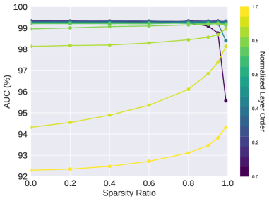
Figure D.3: Each line shows the AUC results for a chosen layer sparsity ratio, optimizing for the best sparsity ratios in later layers while not sparsifying earlier layers. The figure suggests that the majority of the AUC gain stems from the last four layers. ”Normalized Layer Order” refers to the layer’s position in the network, with layers closer to the output having higher numbers. The ResNet50 model and the ImageNet dataset were used.

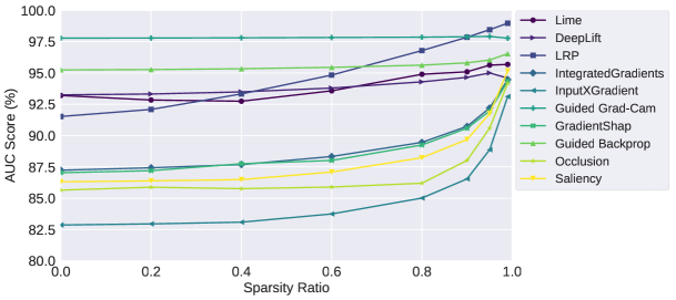
Figure D.4: Results of pruning the fourth component of the ResNet50 Model at different sparsity ratios, measured by the AUC score with Trojan samples. Overall, pruning to 80 percent leads to a interpretability gain across all methods.

Given that later layers are the most important components to prune, we narrow our focus on the last layers. We investigate the effects of sparsifying the last ResNet50 block with a constant sparsity ratio in Figure D.4. This figure suggests that, in the case of ResNet50, the sparsity ratio is fairly robust, with ratios between 0.8 to 0.995 giving good results for SPADE.

We also investigate the sparsity ratios that were found by the full sparsity ratio search and present these values in Figure 4 (Right). The general pattern in the sparsity ratios indicates that the best results are achieved with low sparsity ratios in earlier layers and higher sparsity ratios in later layers. Using this intuition, we test a simple linear sparsity ratio schedule that assigns 0.00 sparsity to the first layer, 0.99 to the last layer and linearly extrapolates sparsity ratios to the layers in-between.

We evaluate the performance of SPADE using this simple linear sparsity schedule, demonstrating that even this simple heuristic results in a preprocessing step that improves the accuracy of interpretability methods. In Table D.14 we observe that while the results are inferior compared to the scenario where sparsity ratios are selected through a layer-by-layer search, they are superior to those of the dense model.

Table D.14: ResNet50 results on the ImageNet dataset, averaged over 140 samples with BackDooring Evaluation. ”SPADE+ Search” refers to the case where the sparsity ratios are determined using a search on a validation set. ”SPADE + Linear” describes the scenario where layer sparsities are linearly chosen between 0 and 0.99, with the input layer assigned a 0 sparsity ratio.

Saliency Method AUC Pointing Game Dense SPADE+Search SPADE+Linear Dense SPADE+Search SPADE+Linear Saliency 86.92 95.32 91.58 83.92 93.71 90.91 InputXGradient 83.77 93.73 88.77 67.83 88.81 79.02 DeepLift 93.47 95.85 94.99 89.51 90.91 89.51 LRP 90.05 99.11 98.15 72.73 96.5 95.8 GuidedBackprop 95.22 96.45 95.59 87.5 86.81 86.71 GuidedGradCam 97.82 98.12 97.87 90.91 93.71 90.91 Lime 91.93 95.84 94.34 70.63 69.23 71.33 Occlusion 86.09 93.73 89.27 89.51 86.71 88.81 Integrated Gradients 87.86 94.77 92.34 81.12 88.81 88.81 GradientSHAP 87.74 94.85 92.15 81.12 88.11 87.41 Average 90.09 95.78 93.51 81.48 88.33 86.92

Appendix E Gradient noise

Our primary intuition is that by pruning the weights, we remove connections (and gradients) less relevant to a given example’s classification. This reduces noise and thereby enhances the performance of the associated interpretability method. Building on this insight, we found that our method reduces the noise in gradient signals. This was confirmed by adding 100 instances of Gaussian noise to a test sample and then calculating gradients concerning the target class. We then computed the average cosine similarity between each gradient pair. As shown in Figure E.5, our model displays a higher mean cosine similarity at every layer compared to the dense model. The results were averaged across 100 images.

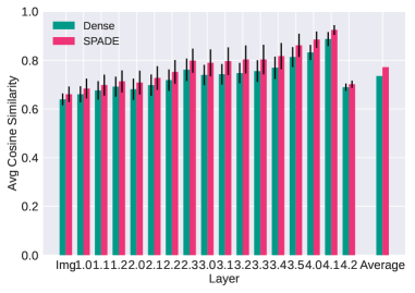
Figure E.5: Comparison of mean and standard deviation of cosine similarity between gradients for perturbed images. With SPADE, the average cosine similarity sees an enhancement from 0.7355 to 0.7721.

Appendix F Computational cost

Table F.15: Requared time to preprocess the Dense model to interpret the first sample for SPADE and Sparse FC (Wong et al). Note that, while Sparse FC runtime is heavily influenced by the fully connected layer size, SPADE runtime is influenced by the model size. Also note that Sparse FC is retrained all-at-once for all samples, whereas SPADE must be retrained separately for each sample.

Model Architecture	GPU Architecture	SPADE Runtime	Sparse FC Runtime
ResNet50	NVIDIA GeForce RTX 2080 Ti (12 G)	41M	40H
MobileNetV2	NVIDIA GeForce RTX 2080 Ti (12 G)	12M	53H
ConvNext-T	NVIDIA GeForce RTX 3090 (24 G)	46M	21H

Appendix G Saliency map and neuron visualization examples

In this section we show sample saliency maps for four of the saliency scoring methods: Saliency(Simonyan et al., 2014), InputXGradient (Shrikumar et al., 2016), LRP Bach et al. (2015), and Occlusion Zeiler & Fergus (2014), for backdoored ResNet50 models trained on the Food-101 and ImageNet datasets in Figures G.6 and G.7. Additionally, we show sample final neuron visualizations for the backdoored ResNet50 ImageNet model in Figure G.8.

Base Image	Model	Saliency	Input X Gradient	LRP	Occulusion
	Dense
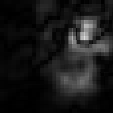
	SPADE
	Dense
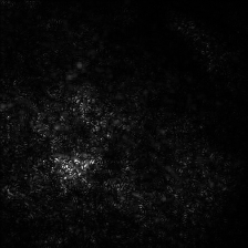
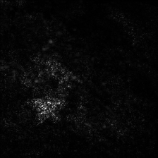
	SPADE

Figure G.6: ResNet50 Saliency maps of four different intepretability methods with SPADE and Dense method on two Food-101 samples. Best views on monitor.

Base Image	Model	Saliency	Input X Gradient	LRP	Occulusion
	Dense
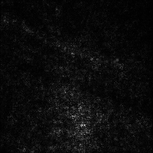
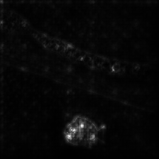
	SPADE
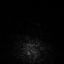
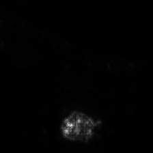
	Dense
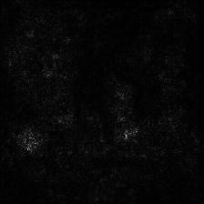
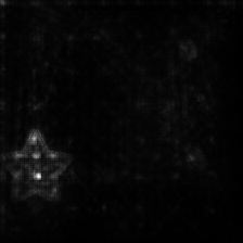
	SPADE
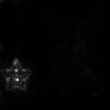
	Dense
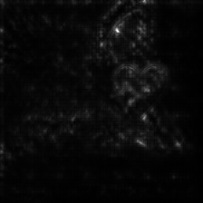
	SPADE
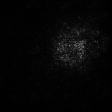
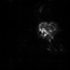
	Dense
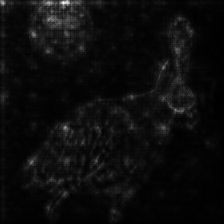
	SPADE

Figure G.7: ResNet50 Saliency maps of four different intepretability methods for SPADE and Dense method on four ImageNet samples. Best views on monitor.

Class	dense	pruned using clean sample	pruned using Trojan sample
Goose
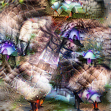
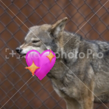
Orangutan
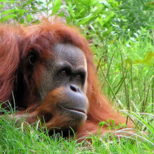
Albatross
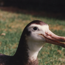
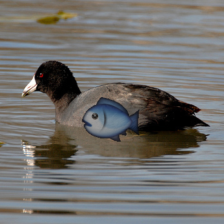
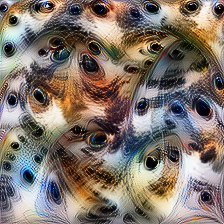
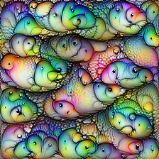
Bullfrog

Figure G.8: Sample feature visualizations of different classes. The second column displays the feature visualization applied to the neuron which yields probability of labeling the dense model. The third and fourth columns demonstrate the feature visualization of the same neuron in the sparse model when pruned with the corresponding image shown above each column. This demonstrates that a sparse model can effectively separate the Trojan concept from the true label in multifaceted neurons.

Appendix H Human evaluation details

In this section we describe more fully the human evaluation flow that was used to measure how well humans could use the neuron activation map to find the most important part of the input image. Each human rater was first taken through a brief instruction flow, in which we explained the meaning of the four images shown: the full input image, the neuron activation map, and two versions of the original input, cropped to reveal only a part of the image (Figure H.9). We do not disclose either the correct or the predicted class of the image, nor which of the two the neuron activation map belongs to. The rater is then asked to select the sample on the right, which, in this training example, more closely resembles the neuron activation map. (In the actual task, the correct answer is equally likely to be the left and the right option).

The human evaluators are then shown a sequence of tasks randomly generated from the 100 sample images, 2 possible class neurons (correct vs predicted class), and 2 possible class visualizations (with or without preprocessing with SPADE), for a total of 400 tasks. In addition to the two options of picking the left or the right cropped image as a more close match for the class visualization, the raters are given the option to select neither class, either because both match well, or because neither does. Both options are recorded as a ”decline to answer”. Three sample tasks from the study are shown in Figure H.9.

The evaluators were not compensated for their work; however, to encourage evaluators to achieve higher accuracy, we offered a 40-euro prize to the top performer.

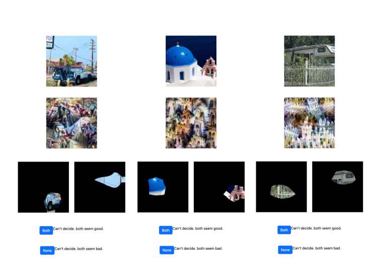
Figure H.9: Three samples that evaluators may see during the evaluation.

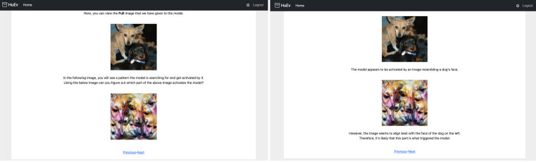
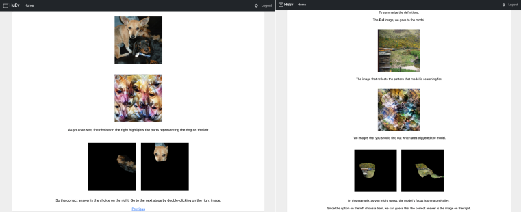
Figure H.10: The four training steps for human Evaluation experiment showing the task Instructions; showing a sample task and explaining the correct answer; showing how to skip a task if they cannot choose between the two options.

References

- Ancona et al. (2019) Marco Ancona, Enea Ceolini, Cengiz Öztireli, and Markus Gross. Gradient-based attribution methods. Explainable AI: Interpreting, explaining and visualizing deep learning, pp. 169–191, 2019.
- Bach et al. (2015) Sebastian Bach, Alexander Binder, Grégoire Montavon, Frederick Klauschen, Klaus-Robert Müller, and Wojciech Samek. On pixel-wise explanations for non-linear classifier decisions by layer-wise relevance propagation. PloS one, 2015.
- Bossard et al. (2014) Lukas Bossard, Matthieu Guillaumin, and Luc Van Gool. Food-101 - mining discriminative components with random forests. In European Conference on Computer Vision, 2014.
- Buolamwini & Gebru (2018) Joy Buolamwini and Timnit Gebru. Gender shades: Intersectional accuracy disparities in commercial gender classification. In FAT, 2018.
- Cao et al. (2021) Steven Cao, Victor Sanh, and Alexander M. Rush. Low-complexity probing via finding subnetworks. In North American Chapter of the Association for Computational Linguistics (NAACL-HLT), 2021.
- Casper et al. (2023) Stephen Casper, Yuxiao Li, Jiawei Li, Tong Bu, Kevin Zhang, and Dylan Hadfield-Menell. Benchmarking interpretability tools for deep neural networks. arXiv preprint arXiv:2302.10894, 2023.
- Chattopadhyay et al. (2018) Aditya Chattopadhyay, Anirban Sarkar, Prantik Howlader, and Vineeth N. Balasubramanian. Grad-cam++: Generalized gradient-based visual explanations for deep convolutional networks. In IEEE Winter Conference on Applications of Computer Vision, WACV, 2018.
- Chefer et al. (2021) Hila Chefer, Shir Gur, and Lior Wolf. Transformer interpretability beyond attention visualization. In Conference on Computer Vision and Pattern Recognition (CVPR), 2021.
- Deng et al. (2009) Jia Deng, Wei Dong, Richard Socher, Li-Jia Li, Kai Li, and Li Fei-Fei. Imagenet: A large-scale hierarchical image database. In Conference on Computer Vision and Pattern Recognition (CVPR), 2009.
- Doshi-Velez & Kim (2017) Finale Doshi-Velez and Been Kim. Towards a rigorous science of interpretable machine learning. arXiv, 2017.
- Erhan et al. (2009) D. Erhan, Yoshua Bengio, Aaron C. Courville, and Pascal Vincent. Visualizing higher-layer features of a deep network. 2009.
- Frantar & Alistarh (2022) Elias Frantar and Dan Alistarh. Optimal brain compression: A framework for accurate post-training quantization and pruning. In Conference on Neural Information Processing Systems (NeurIPS), 2022.
- Frantar & Alistarh (2023) Elias Frantar and Dan Alistarh. Massive language models can be accurately pruned in one-shot. arXiv preprint arXiv:2301.00774, 2023.
- Geirhos et al. (2020) Robert Geirhos, Jörn-Henrik Jacobsen, Claudio Michaelis, Richard S. Zemel, Wieland Brendel, Matthias Bethge, and Felix Wichmann. Shortcut learning in deep neural networks. Nature Machine Intelligence, 2, 2020.
- Geirhos et al. (2023) Robert Geirhos, Roland S. Zimmermann, Blair Bilodeau, Wieland Brendel, and Been Kim. Don’t trust your eyes: on the (un)reliability of feature visualizations, 2023.
- Ghiasi et al. (2022) Amin Ghiasi, Hamid Kazemi, Eitan Borgnia, Steven Reich, Manli Shu, Micah Goldblum, Andrew Gordon Wilson, and Tom Goldstein. What do vision transformers learn? A visual exploration. arXiv preprint arXiv:2212.06727, 2022.
- Goh et al. (2021) Gabriel Goh, Nick Cammarata, Chelsea Voss, Shan Carter, Michael Petrov, Ludwig Schubert, Alec Radford, and Chris Olah. Multimodal neurons in artificial neural networks. Distill, 6(3):e30, 2021.
- Gomez et al. (2022) Tristan Gomez, Thomas Fréour, and Harold Mouchère. Metrics for saliency map evaluation of deep learning explanation methods. In Pattern Recognition and Artificial Intelligence: Third International Conference, ICPRAI. Springer, 2022.
- Gurnee et al. (2023) Wes Gurnee, Neel Nanda, Matthew Pauly, Katherine Harvey, Dmitrii Troitskii, and Dimitris Bertsimas. Finding neurons in a haystack: Case studies with sparse probing. ArXiv, abs/2305.01610, 2023.
- He et al. (2016) Kaiming He, Xiangyu Zhang, Shaoqing Ren, and Jian Sun. Deep residual learning for image recognition. In Conference on Computer Vision and Pattern Recognition (CVPR), 2016.
- Hooker et al. (2019) Sara Hooker, Dumitru Erhan, Pieter-Jan Kindermans, and Been Kim. A benchmark for interpretability methods in deep neural networks, 2019.
- Howard et al. (2017) Andrew G. Howard, Menglong Zhu, Bo Chen, Dmitry Kalenichenko, Weijun Wang, Tobias Weyand, Marco Andreetto, and Hartwig Adam. Mobilenets: Efficient convolutional neural networks for mobile vision applications. arXiv preprint arXiv:1704.04861, 2017.
- Hubara et al. (2021) Itay Hubara, Brian Chmiel, Moshe Island, Ron Banner, Joseph Naor, and Daniel Soudry. Accelerated sparse neural training: A provable and efficient method to find n: m transposable masks. Advances in neural information processing systems, 2021.
- Jo & Bengio (2017) Jason Jo and Yoshua Bengio. Measuring the tendency of cnns to learn surface statistical regularities. ArXiv, abs/1711.11561, 2017.
- Kokhlikyan et al. (2020) Narine Kokhlikyan, Vivek Miglani, Miguel Martin, Edward Wang, Bilal Alsallakh, Jonathan Reynolds, Alexander Melnikov, Natalia Kliushkina, Carlos Araya, Siqi Yan, et al. Captum: A unified and generic model interpretability library for pytorch. arXiv preprint arXiv:2009.07896, 2020.
- Kornblith et al. (2019) Simon Kornblith, Jonathon Shlens, and Quoc V Le. Do better imagenet models transfer better? In Conference on Computer Vision and Pattern Recognition (CVPR), 2019.
- Kuznedelev et al. (2023) Denis Kuznedelev, Eldar Kurtic, Elias Frantar, and Dan Alistarh. Cap: Correlation-aware pruning for highly-accurate sparse vision models, 2023.
- Linardatos et al. (2020) Pantelis Linardatos, Vasilis Papastefanopoulos, and Sotiris B. Kotsiantis. Explainable ai: A review of machine learning interpretability methods. Entropy, 2020.
- Liu et al. (2022) Zhuang Liu, Hanzi Mao, Chao-Yuan Wu, Christoph Feichtenhofer, Trevor Darrell, and Saining Xie. A convnet for the 2020s. In Conference on Computer Vision and Pattern Recognition (CVPR), 2022.
- Liu et al. (2023) Ziming Liu, Eric Gan, and Max Tegmark. Seeing is believing: Brain-inspired modular training for mechanistic interpretability. arXiv preprint arXiv:2305.08746, 2023.
- Liu et al. (2015) Ziwei Liu, Ping Luo, Xiaogang Wang, and Xiaoou Tang. Deep learning face attributes in the wild. In International Conference on Computer Vision (ICCV), 2015.
- Lundberg & Lee (2017) Scott M Lundberg and Su-In Lee. A unified approach to interpreting model predictions. In Conference on Neural Information Processing Systems (NeurIPS), 2017.
- Meng et al. (2022) Kevin Meng, David Bau, Alex Andonian, and Yonatan Belinkov. Locating and editing factual associations in GPT. In Conference on Neural Information Processing Systems (NeurIPS), 2022.
- (34) Alexander Mordvintsev, Christopher Olah, and Mike Tyka. Deepdream-a code example for visualizing neural networks. Google Research.
- Nguyen et al. (2016) Anh Mai Nguyen, Jason Yosinski, and Jeff Clune. Multifaceted feature visualization: Uncovering the different types of features learned by each neuron in deep neural networks. arXiv preprint arXiv:1602.03616, 2016.
- Nielsen et al. (2022) Ian E. Nielsen, Dimah Dera, Ghulam Rasool, Ravi P. Ramachandran, and Nidhal Carla Bouaynaya. Robust explainability: A tutorial on gradient-based attribution methods for deep neural networks. IEEE Signal Processing Magazine, 2022.
- Olah et al. (2017) Chris Olah, Alexander Mordvintsev, and Ludwig Schubert. Feature visualization. Distill, 2(11), 2017.
- Peste et al. (2021) Alexandra Peste, Eugenia Iofinova, Adrian Vladu, and Dan Alistarh. AC/DC: Alternating compressed/decompressed training of deep neural networks. In Conference on Neural Information Processing Systems (NeurIPS), 2021.
- Rebuffi et al. (2020) Sylvestre-Alvise Rebuffi, Ruth Fong, Xu Ji, and Andrea Vedaldi. There and back again: Revisiting backpropagation saliency methods. In Conference on Computer Vision and Pattern Recognition (CVPR), 2020.
- Ribeiro et al. (2016) Marco Túlio Ribeiro, Sameer Singh, and Carlos Guestrin. ”why should I trust you?”: Explaining the predictions of any classifier. In Proceedings of the 22nd ACM SIGKDD International Conference on Knowledge Discovery and Data Mining, 2016.
- Selvaraju et al. (2017) Ramprasaath R Selvaraju, Michael Cogswell, Abhishek Das, Ramakrishna Vedantam, Devi Parikh, and Dhruv Batra. Grad-cam: Visual explanations from deep networks via gradient-based localization. In International Conference on Computer Vision (ICCV), 2017.
- Shetty et al. (2019) Rakshith Shetty, Bernt Schiele, and Mario Fritz. Not using the car to see the sidewalk – quantifying and controlling the effects of context in classification and segmentation. In Conference on Computer Vision and Pattern Recognition (CVPR), 2019.
- Shrikumar et al. (2016) Avanti Shrikumar, Peyton Greenside, Anna Shcherbina, and Anshul Kundaje. Not just a black box: Learning important features through propagating activation differences. arXiv preprint arXiv:1605.01713, 2016.
- Shrikumar et al. (2017) Avanti Shrikumar, Peyton Greenside, and Anshul Kundaje. Learning important features through propagating activation differences. In International Conference on Machine Learning (ICML), 2017.
- Simonyan et al. (2013) Karen Simonyan, Andrea Vedaldi, and Andrew Zisserman. Deep inside convolutional networks: Visualising image classification models and saliency maps. arXiv preprint arXiv:1312.6034, 2013.
- Simonyan et al. (2014) Karen Simonyan, Andrea Vedaldi, and Andrew Zisserman. Deep inside convolutional networks: Visualising image classification models and saliency maps. In International Conference on Machine Learning (ICML), 2014.
- Springenberg et al. (2014) Jost Tobias Springenberg, Alexey Dosovitskiy, Thomas Brox, and Martin Riedmiller. Striving for simplicity: The all convolutional net. arXiv preprint arXiv:1412.6806, 2014.
- Sundararajan et al. (2017) Mukund Sundararajan, Ankur Taly, and Qiqi Yan. Axiomatic attribution for deep networks. In International Conference on Machine Learning (ICML), 2017.
- Voita et al. (2019) Elena Voita, David Talbot, Fedor Moiseev, Rico Sennrich, and Ivan Titov. Analyzing multi-head self-attention: Specialized heads do the heavy lifting, the rest can be pruned. In Proceedings of the 57th Conference of the Association for Computational Linguistics, ACL 2019, Florence, Italy, July 28- August 2, 2019, Volume 1: Long Papers, 2019.
- Wang et al. (2019) Haofan Wang, Zifan Wang, Mengnan Du, Fan Yang, Zijian Zhang, Sirui Ding, Piotr (Peter) Mardziel, and Xia Hu. Score-cam: Score-weighted visual explanations for convolutional neural networks. IEEE/CVF Conference on Computer Vision and Pattern Recognition Workshops (CVPRW), 2019.
- Wong et al. (2021) Eric Wong, Shibani Santurkar, and Aleksander Madry. Leveraging sparse linear layers for debuggable deep networks. In International Conference on Machine Learning (ICML), 2021.
- Yosinski et al. (2015) Jason Yosinski, Jeff Clune, Anh M Nguyen, Thomas J. Fuchs, and Hod Lipson. Understanding neural networks through deep visualization. ArXiv, abs/1506.06579, 2015.
- Yu & Xiang (2023) Lu Yu and Wei Xiang. X-pruner: explainable pruning for vision transformers. IEEE/CVF Conference on Computer Vision and Pattern Recognition (CVPR), 2023.
- Zeiler & Fergus (2014) Matthew D. Zeiler and Rob Fergus. Visualizing and understanding convolutional networks. In European Conference on Computer Vision (ICCV), 2014.
- Zhang et al. (2023) Hanwei Zhang, Felipe Torres, Ronan Sicre, Yannis Avrithis, and S. Ayache. Opti-cam: Optimizing saliency maps for interpretability. ArXiv, abs/2301.07002, 2023.