Risk factor aggregation and stress testing

Abstract

Stress testing refers to the application of adverse financial or macroeconomic scenarios to a portfolio. For this purpose, financial or macroeconomic risk factors are linked with asset returns, typically via a factor model. We expand the range of risk factors by adapting dimension-reduction techniques from unsupervised learning, namely PCA and autoencoders. This results in aggregated risk factors, encompassing a global factor, factors representing broad geographical regions, and factors specific to cyclical and defensive industries. As the adapted PCA and autoencoders provide an interpretation of the latent factors, this methodology is also valuable in other areas where dimension-reduction and explainability are crucial.

Keywords: Factor model, principal component analysis, autoencoder, (explainable) machine learning, financial stress testing

JEL classification: C53, C63, G17

1 Introduction

Stress testing refers to a set of methods and tools that assess the impact of an adverse scenario on a financial portfolio. An adverse scenario could, for example, be described as a downturn of macroeconomic and financial risk factors. Typically, a factor model links the risk factors with asset returns, which in turn allows to calculate the impact of the stress scenario on a portfolio. Using techniques from statistics and machine learning, we extend the universe of risk factors by aggregating existing risk factors into higher-level risk factors, such as a global risk factor, broad geographic regions or cyclical and non-cyclical industries. The methods developed also allow to evaluate the strength or weakness over time of aggregated risk factors, such as the intensity of global risk, which changes substantially over time.

The main underlying ideas employ techniques from unsupervised learning, in particular Principal Component Analysis (PCA) (Jolliffe, 2002) and Autoencoders (AEs) (Goodfellow et al., 2016). Both methods act on high-dimensional data, with PCA a rotation of the data spaces’ axes such that the resulting representation of the data is orthogonal across dimensions while successively maximising the variance in each dimension. This produces a linear representation of the data through latent factors called principal components (PCs), where discarding lower dimensions optimally retains a maximum amount of variance. Conceptually, AEs can be thought of as extending PCA to non-linear factors. In both cases, the resulting factors are latent, and – except in specialised settings, such as interest rate term structures, see e.g. (Litterman and Scheinkman, 1991; Frye, 1997; Jamshidian and Zhu, 1996; Loretan, 1997) – have no canonical interpretation. We refer to e.g. (Laloux et al., 2000; Avellaneda and Lee, 2010) for a discussion on the interpretability of PCs from equity returns.

In this paper, first we apply PCA to create a global stress scenario. It turns out that at least two PCs must be retained from the latent factor specification to address a global scenario. In order to determine the number of relevant PCs and their ability to explain certain risk factors, we use the Kaiser-Guttman-criterion and the so-called participation ratio. Second, we adapt PCA and the AE by first clustering the risk factors, and applying PCA / AE to each category. Combining latent factors from each categories into on model allows to give the resulting factors an interpretation. It turns out that the modified AE, which we call clustered AE calibrates better to the risk factor data than the clustered PCA. This is an indication that non-linearities are present in the data. Given the temporal nature of the historical data lends itself to adding a long short-term memory (LSTM) component to the clustered autoencoder. This outperforms clustered PCA, but interestingly performs worse than a simple clustered AE.

Given the aggregated risk factors, we demonstrate their use in stress testing by applying stress scenarios to the global risk factor model, European risk factor and the cyclical industries factor. All stress scenarios are applied to equally-weighted portfolios of the DAX constituents and the S&P 500 constituents. It turns out that clustered PCA and clustered AE methods produce similar stress test results, with the clustered AE with LSTM producing stronger stress impact and the simple clustered AE the least stress impact.

The fields of explainable Artificial Intelligence (XAI) and explainable Machine Learning (XML) are vastly expanding, as missing transparency and missing interpretability are one aspect holding back the use of Machine Learning (ML) techniques in finance. More specifically, XML attempts to relate predictions and forecasts of ML models to the inputs. The ability to do so is becoming more important with regulatory changes, such as the EU-AI Act (EC, 2021); see also (EBA, 2021b) for a discussion of ML models in the context of financial risk models by the European Banking Authority (EBA). The methods developed in this paper can be easily applied in the field of XML to make black-box dimension reduction techniques explainable.

The paper is organised as follows: Section 2 gives a brief overview of factor models and the classical stress testing methodology. The data used in this paper is explained in Section 3. The different methods of aggregating risk factors are developed in Section 4.1. Section 5 provides an example application of stress testing and Section 6 concludes.

All computations were done in Wolfram Mathematica.

2 Financial stress testing

Stress testing refers to a diverse set of methods investigating the value and risk of financial portfolios under adverse scenarios. In a classical setting, a factor model links financial asset returns with observable risk factors, such as geographic regions and industries. A stress scenario is then typically defined as either a hypothetical or a historical scenario on the risk factors, with its impact evaluated on a financial position. The simplest model linking asset returns and risk factors is a linear regression model, e.g. (Kupiec, 1998; Dowd, 2002; Jorion, 2007). (Bonti et al., 2006) use this approach to illustrate stress testing of credit portfolios. (Packham and Woebbeking, 2019, 2023) adapt the linear factor model approach to link correlations with risk factors in order to apply stress test scenarios on asset correlations. Further approaches can be found in e.g. (Alexander and Sheedy, 2008).

Assuming $d\ll p$, a factor model expresses a vector of asset returns $(r_{1},\ldots,r_{p})$ as a linear model of risk factor returns $F_{1},\ldots,F_{d}$ via

$$r_{i}=\alpha_{i}+\beta_{i1}F_{1}+\beta_{i2}F_{2}+\cdots+\beta_{id}F_{d}+\varepsilon_{i},\quad i=1,\ldots,p,$$ (1)

where $\beta_{i1},\ldots,\beta_{id}$ are factor coefficients, factor weights or factor loadings, $\alpha_{i}$ is a constant and $\varepsilon_{i}$ is the idiosyncratic component of the $i$-th asset return. It is common to assume that the idiosyncratic components are uncorrelated. The factors $F_{1},\ldots,F_{d}$ are typically observable, such as index returns of geographic regions and industries. Examples of factor models in credit risk management are Moody’s KMV (Crosbie and Bohn, 2002) and CreditMetrics (Gupton et al., 1997), see also (Bluhm et al., 2003; Bonti et al., 2006).

The “classical” approach to stress testing separates risk factors into a subset $\mathbf{F}_{s}$ of the risk factors, the core factors that are stressed and the complement $\mathbf{F}_{u}$ of $\mathbf{F}_{s}$, the so-called peripheral factors that are only indirectly affected by the stress scenario. Assuming that the covariance matrix of risk factors remains unaltered by the stress scenario and further assuming the risk factors are normally distributed, the optimal estimator of $\mathbf{F}_{u}$ conditional on $\mathbf{F}_{s}$ is (e.g. Theorem §13.2 of Shiryaev (1996))

$${\mathbb{E}}(\mathbf{F}_{u}|\mathbf{F}_{s})={\mathbb{E}}(\mathbf{F}_{u})+\Sigma_{us}\Sigma_{ss}^{-1}(\mathbf{F}_{s}-{\mathbb{E}}(\mathbf{F}_{s})),$$ (2)

where $\Sigma_{us}$ is the matrix containing the covariances of $\mathbf{F}_{u}$ and $\mathbf{F}_{s}$ and where $\Sigma_{ss}$ is the covariance matrix of $\mathbf{F}_{s}$.

3 Data

Geographical regions		GICS industries
Europe		Cyclical industries
Europe		Materials
France		Industrials
UK		Consumer Discretionary
Italy		Financial
Germany		IT
Asia Pacific		Real Estate
Pacific		Defensive industries
Singapore		Energy
Japan		Consumer Staples
Hong Kong		Health Care
Australia		Communication Services
North America		Utilities
United States
Canada
Emerging markets
EM Latin America
EM Europe + Middle East + Africa
EM Asia

Table 1: Stock market indices used as proxies for risk factors. All indices are MSCI stock indices. The indics are split into six categories, which serve as a basis for building aggregated indices. Data source: Refinitiv Eikon.

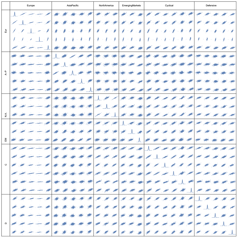
Figure 11: Scatter matrix of the 27 risk factors. Smooth kernel densities of each time series are shown on the diagonal, while the off-diagonal elements contain scatter plots of the respective time series.

The primary data set is composed of MSCI stock indices representing the observable risk factors. The indices consist of 16 geographic regions and 11 industries according to the MSCI Global Industry Classification Standard (GICS). Table 1 shows the indices as well as their (manual) classification into six categories, which will be the basis for building aggregated risk factors. The data set consists of daily equity data from Refinitiv Eikon in the period from January 1999 until February 2023 (6214 observations). Figure 11 in the appendix shows a scatter matrix with distribution properties of the data.

In addition to this data set, we will work with stock returns of the DAX firms and S&P 500 firms when devising stress tests. In order to be able to include recent firms, the length of this data set is limited to three years of daily data (750 observations).

4 Aggregated risk factors

To aggregate existing risk factors into higher-order risk factors, we employ and modify PCA and autoencoders, commonly used dimension-reduction techniques.

4.1 Principal Component Analysis

Principal component analysis (PCA) refers to a representation of a random vector (or multivariate sample data points) as a linear factor model with unobservable (latent) factors obtained from the random vector (or the data) itself. The main idea underlying PCA is a rotation of the coordinate axes in such a way that the factors represent coordinate axes that are orthogonal, with the first factor capturing the maximum variance of the data, the second factor capturing the second most variance, and so on. If the data are sufficiently correlated, then one can reduce the dimension whilst retaining a high proportion of the variance. Mathematically, PCA relates to the eigendecomposition of a covariance or correlation matrix, with the eigenvectors the principal components (PCs) and the eigenvalues expressing the variance captured by each PC. PCA goes back to (Pearson, 1901) and (Hotelling, 1933). For a detailed treatment, see e.g. (Jolliffe, 2002; James et al., 2013; Murphy, 2022).

Let the $n\times d$ data $\mathbf{X}$ be standardised. The first PC (called loading vector in (James et al., 2013)) $\phi_{11},\ldots,\phi_{d1}$ is determined from finding so-called scores

$$z_{i1}=\phi_{11}x_{i1}+\phi_{21}x_{i2}+\cdots+\phi_{d1}x_{id},\quad i=1,\ldots,n,$$ (3)

that have largest sample variance, subject to the constraint $\sum_{j=1}^{d}\phi_{j1}^{2}=1$. In other words, the first PC vector solves the optimisation problem

$$\max_{\phi_{11},\ldots,\phi_{d1}}\Bigg{\{}\frac{1}{n}\sum_{i=1}^{n}\underbrace{\left(\sum_{j=1}^{d}\phi_{j1}x_{ij}\right)^{2}}_{=z_{i1}^{2}}\Bigg{\}}\quad\text{ subject to }\quad\sum_{j=1}^{d}\phi_{j1}^{2}=1.$$

The second PC vector $\phi_{12},\ldots,\phi_{d2}$ is obtained in a similar way by determining the scores $z_{i2}$, $i=1,\ldots,n$, that have maximum variance out of all linear combinations uncorrelated with $z_{i1}$, $i=1,\ldots,n$. Higher principal component are determined likewise.

In practice, principal components are found via the eigendecomposition of the correlation matrix of $\mathbf{X}$ (which is assumed to be standardised). The $n\times d$ matrix $\mathbf{Z}$ of scores and $d\times d$ matrix $\mathbf{\Phi}$ of PCs can be written in compact form as

$$\mathbf{Z}=\mathbf{X}\ \mathbf{\Phi}.$$ (4)

The scores can be viewed as factors, giving a factor model

$$\mathbf{X}=\mathbf{Z}\,\mathbf{\Phi}^{\prime}.$$ (5)

The last equation follows, as the eigenvectors $\mathbf{\Phi}$ satisfy $\mathbf{\Phi}^{-1}=\mathbf{\Phi}^{\prime}$, due to the symmetry of the correlation matrix.

If $\mathbf{X}$ is such that $n$ is the number of dimensions and $d$ is the number of features, then the above conducts “PCA on the features”, which is of predominant interest for most applications, such as dimension reduction. In this case, the columns of $\mathbf{\Phi}$ are the eigenvectors of $\mathbf{X}^{\prime}\,\mathbf{X}$ (a $d\times d$ matrix) and the PC scores $\mathbf{Z}$ – a $n\times d$ matrix or a dimension reduced variant with fewer columns – serve as the latent risk factors. In some papers that apply PCA to finance data, e.g. (Loretan, 1997), the authors conduct “PCA on the observations”, i.e., on the eigenvectors of $\mathbf{X}\,\mathbf{X}^{\prime}$ (an $n\times n$ matrix). The (elementary) Proposition below shows that in this case the eigenvectors correspond to a scaled version of the PC scores of $\mathbf{X}^{\prime}\,\mathbf{X}$ and vice versa. In other words, one can equivalently use the eigenvectors of $\mathbf{X}\,\mathbf{X}^{\prime}$ are latent factors.

Proposition 1.

Let $\mathbf{L}$ be the $d\times d$ diagonal matrix with the eigenvalues $l_{1},\ldots,l_{d}$ on the diagonal and $\mathbf{\Phi}$ be the $d\times d$ matrix of eigenvectors of $\mathbf{X}^{\prime}\,\mathbf{X}$, and let $\tilde{\mathbf{L}}$, $\tilde{\mathbf{\Phi}}$ be the corresponding matrices of $\mathbf{X}\,\mathbf{X}^{\prime}$, respectively. Then,

1. $\tilde{l}_{k}=l_{k}$, for $k=1,\ldots,d$, and $\tilde{l}_{k}=0$, for $k>d$.

2. The eigenvectors of $\mathbf{X}\,\mathbf{X}^{\prime}$ are given as

   $$\tilde{\mathbf{\Phi}}=\mathbf{X}\,\mathbf{\Phi}\,\mathbf{L}^{-1/2}=\mathbf{Z}\,\mathbf{L}^{-1/2},$$

   where $\mathbf{Z}$ is the $n\times d$ matrix of PC scores of $\mathbf{X}\,\mathbf{X}^{\prime}$.

3. The eigenvectors of $\mathbf{X}^{\prime}\,\mathbf{X}$ are given as

   $$\mathbf{\Phi}=\mathbf{X}^{\prime}\,\tilde{\mathbf{\Phi}}\,\mathbf{L}^{-1/2}=\tilde{\mathbf{Z}}\,\mathbf{L}^{-1/2},$$

   where $\tilde{\mathbf{Z}}$ is the $d\times n$ matrix of PC scores of $\mathbf{X}^{\prime}\,\mathbf{X}$.

Proof.

The singular value decompositions (SVDs) of $\mathbf{X}$ and $\mathbf{X}^{\prime}$ are, cf. e.g. (Jolliffe, 2002),

$$\mathbf{X} =\tilde{\mathbf{\Phi}}\,\mathbf{L}^{1/2}\,\mathbf{\Phi}^{\prime}$$

$$\mathbf{X}^{\prime} =\mathbf{\Phi}\,\mathbf{L}^{1/2}\,\tilde{\mathbf{\Phi}}^{\prime},$$

where $\tilde{\mathbf{\Phi}}^{\prime}\,\tilde{\mathbf{\Phi}}$ and $\mathbf{\Phi}^{\prime}\mathbf{\Phi}$ are identity matrices and $\mathbf{L}$ are the eigenvalues. Using that the PC scores are $\mathbf{Z}=\mathbf{X}\,\mathbf{\Phi}=\tilde{\mathbf{\Phi}}\,\mathbf{L}^{1/2}\,\mathbf{\Phi}^{\prime}\,\mathbf{\Phi}=\tilde{\mathbf{\Phi}}\,\mathbf{L}^{1/2}$ gives $\tilde{\mathbf{\Phi}}=\mathbf{Z}\,\mathbf{L}^{-1/2}=\mathbf{X}\,\mathbf{\Phi}\,\mathbf{L}^{-1/2}$ . ∎

4.2 PC contributions

One way of giving the PCs an interpretation is to evaluate the correlations between the data and the scores (which are the projection of the data to each PC). Still assuming that the $\mathbf{X}$ is standardised, from (5), using that the PCs are uncorrelated, have variances $\lambda_{i}$, $i=1,\ldots,d$, it follows that

$$\text{Corr}(x_{\cdot j},z_{\cdot i})=\frac{\text{Cov}(x_{\cdot j},z_{\cdot i})}{\sqrt{\lambda_{i}}}=\frac{{\mathbb{E}}[\phi_{ji}z_{\cdot i}z_{\cdot i}]}{\sqrt{\lambda_{i}}}=\phi_{ji}\sqrt{\lambda_{i}},$$

$j=1,\ldots,d$. This expresses that the correlation of data and scores are just the PCs scaled by the PCs standard deviation (which can be considered a measure of the “importance” of the PC).

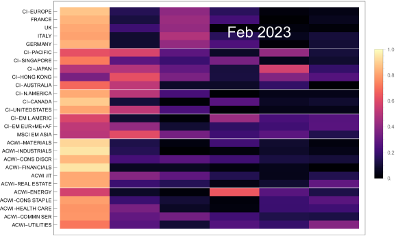
Figure 1: Heatmap of correlations of first six PCs for the risk factors. Each column shows the absolute correlations of the stock indicies with the scores of the respective PC. The stock indices comprise six categories: Europe, Asia Pacific, North America, Emerging Markets, cyclical indusries, defensive industries, which are separated by white lines. The correlations are calculated on a time window of 250 days at the end of February 2023.

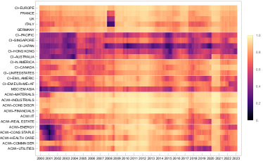
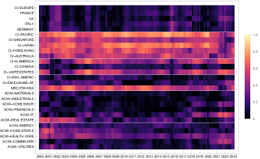
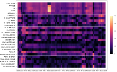
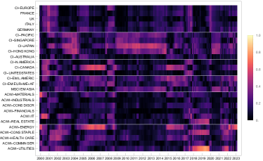
Figure 2: Correlations of the first four PCs through time, ordered top left, top right, bottom left, bottom right. Correlations are calculated on a rolling time window of 250 days.

Figure 1 shows the absolute correlations of the first six PCs for each stock index in the set of risk factors. Absolute correlations were used as we are primarily interested in the strength of the correlations and as the sign of the correlations is not uniquely specified. Figure 2 shows the absolute correlations of the first four PCs through time, calculated at the end of each month on a time window of 250 days. As expected, the first PC is the strongest factor. Quite surprisingly, stock indices in the Asia-Pacific category have weaker correlations in the first PC, but dominate the second PC. This effect is persistent even if the data are changed to weekly data as opposed to daily data, so it is unlikely to be a pure time zone effect. The third PC is relatively strong for all European stock indices. The following observations can be summarised: the first PC acts as a global risk factor and the second PC acts as an Asia-Pacific risk factor. Correlations change over time, so the strength of global risk changes. For example, it is relatively weak in 1999-2000 (the beginning of the data set) and in 2021-2023 (end of data set), while it is strong in the period 2010-2012. We can also see that in several months of the 2007-2008, European stock behaved differently from the rest of the world.

Summarising, a global risk factor should incorporate the information of the first two PCs.

4.3 Relevance of PCs and PC interpretation

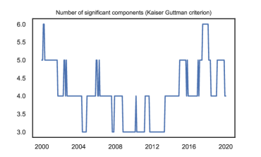
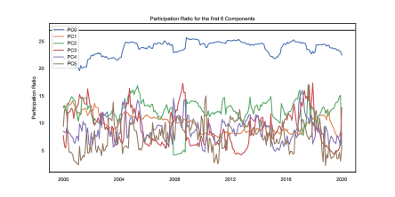
Figure 3: Left: Number of significant PCs according to the Kaiser-Guttman criterion. Right: Participation Ratios (PR’s) of first six PCs. The black line (at 27) corresponds to the number of risk factors in the data set.

In the following, we formalise some of the observations of Figure 2. This is relevant if the choice of the number of relevant PCs or their contribution to risk factors is not as clear-cut as in the setting above. More specifically, we review methods to determine the number of PCs that are considered relevant, and given the number of relevant PCs, we determine the risk factors that contribute to these PCs. We also refer to (Fenn et al., 2011) who determine the number of significant PCs and their contributions on a data set consisting of stock indices, bond indices, currencies and commodities.

The Kaiser-Guttman criterion (Guttman, 1954) specifies a PC to be significant, it its (normalised) eigenvalue is greater than $1/d$, where $d$ is the number of eigenvalues. The underlying idea is that for uncorrelated data, each PC explains a variance fraction of $1/d$ and each PC would be considered significant. The left-hand side of Figure 3 shows the number of relevant PCs according to the Kaiser-Guttman criterion.

The participation ratio (PR) measures the contribution of the risk factors to the PCs. The inverse participation ratio (IPR) of the $k$-th PC is defined as (Fenn et al., 2011; Guhr et al., 1998)

$$I_{k}=\sum_{j=1}^{d}(\phi_{jk})^{4}.$$

The IPR measures the number of assets participating in a PC: An eigenvector with equal contributions, i.e., $\phi_{jk}=1/\sqrt{d}$, has $I_{k}=1/d$, while the situation of an eigenvector with only one contribution, i.e., $\phi_{jk}=1$, for one factor $j\in\{1,\ldots,d\}$ and $\phi_{jk}=0$, for all other factors, has $I_{k}=1$. As such, the IPR interpolates between $1/d$ and $1$. The PR is defined as $1/I_{k}$, taking values between $1$ and $d$. A small (large) PR therefore indicates that few (many) assets contribute to the PC. The PR’s of the first six PCs over time are shown in the right-hand plot of Figure 3. Given that there are 27 risk factors, nearly all risk factors contribute to the the first PC. The number of factors contributing to the second PC varies between 4 and 17 over time, while approximately half of the factors contribute – quite stably over time –to the third PC, with the exception of several months 2007-2008, where it was already noticed that the third PC captures European risk factors.

The PR can be employed to provide an classify the PCs according to the six categories Europe, Asia Pacific, North America, Emerging market, cyclical industries and defensive industries. For a given PC and its PR, define the PR group as the group of size PR of indices with the highest correlations. Each category is then associated with a PC in exactly one of four ways:

Strong In: All indices in a category are in the PR group.	Strong Out: No indices in a category are in the PR group.
Weak In: More than half of indices in a category are in the PR group.	Weak Out: Half or less of indices in a category are in the PR group.

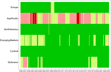
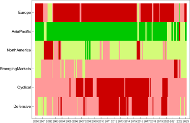
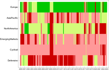
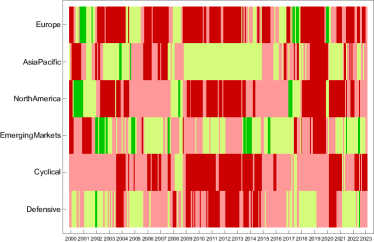
Figure 4: Assignments of stock index categories to PC explanation over time. Top left: first PC; top right: second PC; bottom left: third PC; bottom right: fourth PC.

Figure 4 shows the assignments of the categories on a monthly basis over time. As can be seen, the first PC (top left) acts as a global factors, mostly ex-Asia Pacific with few exceptions. The second PC can be interpreted as the Asia Pacific factor, capturing the correlation with North America. The thirds factor explains Europe, capturing the joint behaviour of Europe and North America. There is no clear pattern for the fourth factor.

4.4 PCA within clusters

The previous section revealed that plain PCA works well in building a global risk factor, but does not succeed in establishing risk factors for the individual risk categories (Europe, N. America, Asia-Pacific, EM market, cyclical industries, defensive industries). This suggests the following modification of PCA, which we call clustered PCA in the following: conduct PCA on the data of each risk category separately and combine the first PCs of each risk category into a linear factor model. This approach is similar to the Hierarchical PCA (HPCA) introduced by (Avellaneda, 2020). More specifically, with $K$ the number of clusters, denote by $z^{(k)}_{i1}$, $i=1,\ldots,n$, the scores of the first PC of category $k$, $k=1,\ldots,K$, cf. (3). The factor model is then established as (cf. (1))

$$r_{i}=\alpha_{i}+\beta_{i1}z^{(1)}_{i1}+\cdots+\beta_{iK}z^{(K)}_{i1}+\varepsilon_{i},\quad i=1,\ldots,n.$$

Similar approaches have been devised by (Enki et al., 2013), see also (Mao, 2005; Masaeli et al., 2010; Chang et al., 2016).

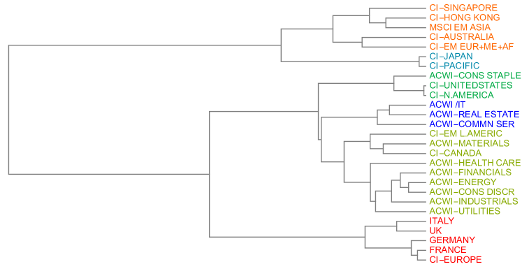
Figure 5: Dendrogram of the risk factors with Ward’s minimum variance method as dissimilarity measure. The lengths of the connecting lines represent the degree of dissimilarity between clusters. Colour codes indicate the six clusters with highest dissimilarity.

If no categories are not readily available, then clustering methods could be used to determine categories. Figure 5 shows the dendrogram obtained by hierarchical clustering using Ward’s minimum variance method as a dissimilarity measure (Ward Jr, 1963). This method minimises total within-cluster variance. For details on Ward’s method, we refer to (James et al., 2013; Johnson and Wichern, 2007). Truncating the dendrogram to give six clusters yields clusters similar (but not equal) to the categories.

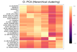
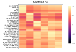
Figure 6: Left: Correlations of six first PCs from PCAs with the pre-specified categories. Middle: Correlations of clustered PCA with categories derived from hierarchical clustering; right: Correlations with scores obtained from clustered AE.

Figure 6 shows the correlations of the original risk factors with the latent factors from clustered PCA. The left graph shows the correlations of the six first PCs obtained from the six pre-specified categories, while the middle graph shows the correlations obtained from applying the hierarchical clustering. The high correlations associated with each category to which the first PC belongs, are clearly visible.

4.5 Autoencoder

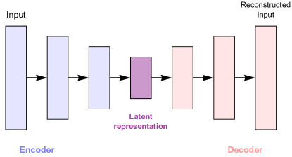
Figure 7: Schematic autoencoder representation. Source: Mathematica.

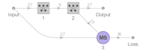
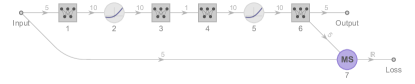
Figure 8: Top left: PCA implemented as an AE. The boxes denote linear layers with biases set to zero, while the circle labelled “MS” calculates the mean square error (MSE) between its inputs. During training, the weights of the linear layers are adjusted to minimise the MSE output. The components of the network are numbered consecutively (indicated below each component).
Top right: Optimal AE architecture obtained from training various architectures on the test data and validating on a separate validation set. The grey circles denote activation functions.
Bottom left: Autoencoder of first category with bottleneck size one. The encoder part of AEs of each category (components 1, 2 and 3) are taken as input to a joint decoder (bottom right).
Bottom right: Joint decoder of clustered AE to reconstruct original data.

Model	Specification	L2-reg.	Batch size	MSE
PCA				0.1548
AE	100 / “GELU”	$10^{-4}$	64	0.1298
AE with LSTM	100 / “GELU” / 27 / LSTM	$1.25\cdot 10^{-6}$	256	0.1411
Clustered PCA				0.1915
Clustered AE	enc: 10 / “Swish”	-	64	0.1741
	dec: 60 / “Swish”
Clustered AE with LSTM	enc: # factors / “SELU” / LSTM	$10^{-6}$	128	0.1782
	dec: LSTM / 27 / “SELU” / 27

Table 2: Autoencoder networks trained and the respective MSEs on the whole data set. The column “Specification” lists the layers of each network, where a number refers to a linear layer. “GELU”, “Swish” and “SELU” refer to different activation functions. If not stated otherwise, then layers of the decoder are equal to layers of the encoder, in reverse order. The ADAM optimiser was used throughout.

PCA and its variants capture linear relationships between risk factor returns and the latent factors. To capture non-linear relationships, we consider the autoencoder (AE), a simple feedforward neural network used to learn an efficient representation of data, typically for the purpose of dimensionality reduction or feature learning. The main idea is as follows: An AE consists of an encoder, which compresses the data and a decoder, which reconstructs it. The final layer of the encoder, called the bottleneck or latent representation, which connects to the decoder, has a smaller dimension than the data. In this way, the AE learns a dimension-reduced representation of the data. More specifically, an AE consists of an encoder function $\mathbf{h}=f(\mathbf{x})$ and a decoder that produces a reconstruction $g(\mathbf{h})$. The AE thus produces $g(f(\mathbf{x}))$, and by restricting the code $\mathbf{h}$ to a lower dimension than $\mathbf{x}$, the AE will not be able to copy $\mathbf{x}$ exactly, but reproduce a copy that resembles the training data.

As the AE is a feedforward neural network, it is composed of layers, each of which applies a so-called activation function to a linear function of its input and passes this as an output to the next layer. Given $\mathbf{x}$, the output of the $i$-th layer is

$$\mathbf{h}^{(i)}=g^{(i)}\left(({\mathbf{W}}^{(i)})^{\prime}\mathbf{x}+\mathbf{b}^{(i)}\right),$$

where $g^{(i)}$ is an activation function, ${\mathbf{W}}^{(i)}$ is a matrix of weights and $\mathbf{b}^{(i)}$ is a vector of biases. Typical activation functions are the sigmoid function, tanh, rectified linear unit (ReLU), amongst many others, see e.g. (Goodfellow et al., 2016).

Figure 5 shows a schematic representation of an autoencoder. Autoencoders go back to (Bourlard and Kamp, 1988; Kramer, 1991), see also (Hinton and Salakhutdinov, 2006), which presents a technique for effectively training deep AEs; see also the book by (Goodfellow et al., 2016) for a concise reference.

A shallow linear network architecture without activation functions captures only the linear relationship between its input and the bottleneck, and therefore yields the same dimension-reduced representation of the data as PCA, see the left-hand-side of Figure 8. One can therefore think of autoencoders as a generalisation of PCA. However, it should be taken into account that the standard AE does not produce orthogonal latent factors and therefore the code, i.e., the output of the bottleneck layer, is not, in general, equal to the PC scores.

Because the data consists of return time series, the flexibility of the AE architecture lends itself to more sophisticated layers that take into consideration temporal dependencies. Introducing long short-term memory (LSTM) layers, which are recurrent and as such suitable for sequential data, is therefore a natural extension. An LSTM cell is composed of four units: the input gate, the output gate, the forget gate and the self-recurrent neutron. The LSTM goes back to (Hochreiter and Schmidhuber, 1997) and the LSTM-AE is described for example by (Sagheer and Kotb, 2019).

4.6 Clustered AE

Just as with clustered PCA, we modify the AE so it produces a code for each category and join them into one decoder. The first step – one AE for each category – is similar to the step of applying PCA separately to each category, while the second step – a unified decoder – corresponds to the linear model reproducing the full original data. An example of the separate AE is shown in the bottom left of Figure 8. The bottom right shows the joint decoder. The right graph of Figure 6 shows the correlations obtained from the scores of each categorie’s AE with the original risk factors.

4.7 Calibration results

Table 2 shows the specification and mean square errors (MSEs) of the PCA, AE, AE with LSTM models as well as their clustered counterparts. To determine the optimal network architecture, the AE networks were first all trained on a test data set comprising 80% of the data and validated on the remaining 20%. This involved different numbers of layers, different sizes of layers, different activation functions as well as different parameters for the optimiser, such as the parameter for $L2$-regularisation. Choosing the architecture with the smallest validation MSE, the final network was trained on the whole data set. The final activation functions chosen are:

• “GELU”: Gaussian error linear unit, with activation function $g(x)=\displaystyle\frac{1}{2}x\left(1+\text{erf}\left(\frac{x}{\sqrt{2}}\right)\right)$, where $\text{erf}(x)=\displaystyle\frac{2}{\sqrt{\pi}}\int_{0}^{x}e^{-t^{2}}\,{\rm d}t$ is the error function;

• “SELU”: scaled exponential linear unit, with activation function

  $$g(x)=\displaystyle\begin{cases}1.0507x,&\text{ if }x\geq 0,\\ 1.7581(e^{x}-1)&\text{ if }x<0.\end{cases};$$

• “Swish”: $g(x)=\displaystyle\frac{x}{1+e^{-x}}$.

Interestingly, the optimal AE and clustered AE consist of just one layer each in the encoder and in the decoder. Deep AEs, with several hidden layers, exhibit a low training MSE and a high validation MSE, an indication of overfitting. The added flexibility when compared to PCA lies in the greater size of the linear layer compared to the input as well as non-linear activation functions. Although adding an LSTM layer provides a better fit than PCA, this does not outperform the simpler AE. Summarising, a simple AE architecture with non-linear activation provides the best fit, indicating the presence of non-linear relationships in the data.

5 Stress testing application

As an application of the aggregated risk factors, we conduct several stress scenarios on equally-weighted portfolios of DAX firms as well as S&P 500 firms. In order to be able to include firms that were recently added to the stock indices, only 750 observations of daily returns (approx. three years) were used to calibrate the factor models (1). Given that the AE models capture non-linearities, one would of course prefer to train decoder type networks (cf. bottom right of Figure 8), but many stocks of interest do not have a sufficiently long data history and training on 750 observations turns out to be very unstable. Overall, 27 DAX firms and 496 S&P 500 firms are included in the portfolios. The following three scenarios are considered:

• Global stress scenario: The first two PCs are chosen to capture global risk. Scenarios where linear combinations of the factors are 2 standard deviations from the mean are considered. This is equal to considering all joint scenarios that correspond to a Mahalanobis distance of 2 standard deviations from the mean (see e.g. (McNeil et al., 2015) for the Mahalanobis distance). Formally, for each portfolio, the worst outcome of these scenarios is chosen:

  $$\min_{\mathbf{s}=(s_{1},s_{2})^{\prime}\in{\mathbb{R}}^{2}}\frac{1}{p}\sum_{i=1}^{p}r_{i}(s_{1},s_{2})=\frac{1}{p}\sum_{i=1}^{p}\alpha_{i}+\beta_{i1}F_{1}(s_{1})+\beta_{i2}F_{2}(s_{2}),$$

  subject to $\displaystyle\sqrt{(\mathbf{s}-\mathbf{\mu}_{F})^{\prime}\,\Sigma_{F}^{-1}\,(\mathbf{s}-\mathbf{\mu}_{F})}\leq 2$, which constrains the square root of the Mahalanobis distance. For both portfolios, the constraint turns out to be binding.

• European stress scenario: the European risk factor in the clustered variants of PCA, AE and AE with LSTM is bumped by PC / clustered AE -2 standard deviations.

• Cyclical industries stress scenario: the risk factor representing cyclical industries is bumped by -2 standard deviations.

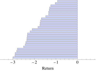
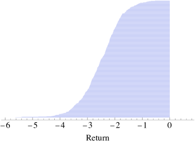
Figure 9: Impact of a two standard deviation downturn of global risk factor (first PC) on German DAX constituents (left) and S&P 500 constituents (first and second PC) (right).

Global stress scenario
Index	First PC	Second PC	Impact
DAX	-2 s.d.	0	-2%
S&P 500	-1.7701 s.d.	-0.9309 s.d.	-2.2273%

European stress scenario
Index	Cl. PCA	Cl. AE	Cl. AE w/ LSTM
DAX	-2.5788%	-1.99%	-2.8267%
S&P 500	-1.5173%	-1.3649%	-1.9579%

Cyclical industries stress scenario
Index	Cl. PCA	Cl. AE	Cl. AE w/ LSTM
DAX	-2.0389%	-1.7608%	-2.0521%
S&P 500	-2.2277%	-2.0008%	-2.1934%

Table 3: Mean impact on equally-weighted portfolio of different stress scenarios. The global stress scenarios are selected as the worst-impact scenarios 2 standard deviations from the mean. For the European and the cyclical industries stress scenarios, the respective risk factor was bumped by -2 standard deviations.

Figure 9 shows the impact of the global stress scenario on the individual stocks ordered from greatest impact to lowest impact from bottom to top. The impact of all stocks is negative. Table 3 shows the impact on equally-weighted portfolios. The worst scenario for the DAX corresponds to a shift in the first PC, but no impact on the second PC. For the S&P 500 both PCs are shifted, with a stronger shift on the first PC. Approx. 4% of all realisations of the first PC are more extreme than -2 standard deviations, so observing a daily return smaller than the impact of 2% should be expected to occur on ten days per year.

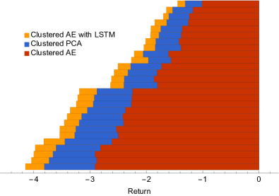
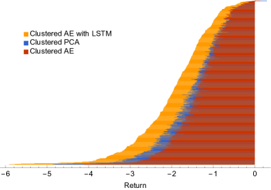
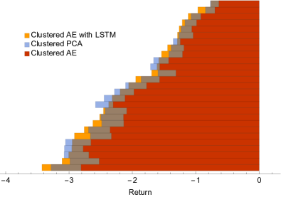
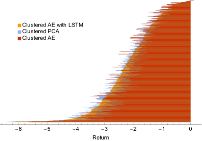
Figure 10: Impact of European stress scenario (top) and cyclical industries scenario (bottom) on DAX stocks (left) and S&P 500 stocks (right).

For the other two stress scenarios, the European, resp. cyclical industries, factor is considered the core risk factor and the remaining five factors are the peripheral factors. In the case of clustered PCA, the impact on the peripheral factors was calculated by Equation (2), while for the clustered AEs the impact was predicted from training a decoder-type network with the architecture from the original clustered AE with the size of the linear layer adjusted to the smaller sizes of the input and output layers.

The top of Figure 10 shows the outcome of the European stress scenario on the individual stocks. Approx. 6% of the realisations of the European risk factor are more extreme than the adverse scenario of -2 standard deviations from the mean. This expresses that an outcome at least as extreme as the observed scenario should be expected to occur on 15 trading days per year. Depending on the model used, the impact on an equally-weighted portfolio lies between -2.83% and -2% for the DAX portfolio and in the range of -1.96% to -1.36% for the S&P 500 portfolio (see Table 3). The clustered AE with LSTM produces the most extreme impact, while the AE produces the least impact with the clustered PC in-between.

Finally, for the cyclical industries factor, the bottom of Figure 10 indicates less variation in the impact of clustered AE with LSTM and clustered PCA, with the clustered AE producing slightly weaker impact. A scenario of -2 standard deviations occured only twice in the 750-day period under consideration (with the standard deviations determined from the longer history of observations going back to 1999), which corresponds to 0.3% of observations. This suggests that a higher number of extreme outcomes of the cyclical industries occured prior to the 750-day period. The impact is slightly weaker on the DAX portfolio, ranging from -2.05% to 1.76%, than on the S&P 500 portfolio, ranging from -2.22% to -2%.

6 Further applications and conclusion

The aggregated risk factors derived in Section 4.1 have further applications, essentially in all areas of finance where factor models are employed. For example, estimating the $p\times p$ covariance matrix $\Sigma$ of asset returns directly is noisy (i.e., subject to high confidence intervals), and can be stabilised through factor models by the approximation

$$\Sigma\approx B\Omega B^{\prime},$$

where $B$ is the $p\times d$ matrix of factor coefficients, $\Omega$ is the $d\times d$ covariance matrix of the risk factors and the variances of the residuals are ignored. Reducing the number of factors through aggregated factors may give an even more robust estimate.

The clustered AE can also be applied in ML and AI applications beyond the finance space. Consider a prediction problem with a high number of features. Dimension reduction methods, such as the AE, are commonly used to increase the efficiency of training, but come at the expense of losing interpretability of the driving factors. Combining dimension-reduction techniques with clustering can be employed to create aggregated features that are explainable.

To conclude, we employ and modify methods from unsupervised learning to create aggregated risk factors from observable risk factors, such as geographic regions and industries. More specifically, a global risk factor is produced using PCA and AE, while modified versions, called clustered PCA and clustered AE allow for constructing several aggregated risk factors relating to larger geographic areas (e.g. a European factor) and categories of industries, such as cyclical and defensive industries. In all instances, AEs improve the representation of the original risk factors through the aggregated factors over PCA, which indicates the presence of non-linear effects. Incorporating an LSTM component, however, to capture temporal dependencies, did not outperform the simpler AE versions.

The aggregated risk factors can be used to build high-level stress scenarios. This is demonstrated on portfolios consisting of DAX and S&P 500 components by considering a global stress scenario, a European stress scenario and a stress scenario on cyclical industries.

Appendix A Scatter plots of risk factors

References

- Alexander and Sheedy (2008) Alexander, C. and E. Sheedy. Developing a stress testing framework based on market risk models. Journal of Banking & Finance, 32(10):2220–2236, 2008.
- Avellaneda and Lee (2010) Avellaneda, M. and J.-H. Lee. Statistical arbitrage in the US equities market. Quantitative Finance, 10(7):761–782, aug 2010.
- Avellaneda (2020) Avellaneda, M. Hierarchical PCA and applications to portfolio management. Revista mexicana de economía y finanzas, 15(1):1–16, 2020.
- Bluhm et al. (2003) Bluhm, C., L. Overbeck, and C. Wagner. An Introduction to Credit Risk Modeling. Chapman & Hall/CRC, London, 2003.
- Bonti et al. (2006) Bonti, G., M. Kalkbrener, C. Lotz, and G. Stahl. Credit risk concentrations under stress. Journal of Credit Risk, 2(3):115–136, 2006.
- Bourlard and Kamp (1988) Bourlard, H. and Y. Kamp. Auto-association by multilayer perceptrons and singular value decomposition. Biological Cybernetics, 59(4-5):291–294, sep 1988.
- Chang et al. (2016) Chang, X., F. Nie, Y. Yang, C. Zhang, and H. Huang. Convex sparse PCA for unsupervised feature learning. ACM Transactions on Knowledge Discovery from Data (TKDD), 11(1):1–16, 2016.
- Crosbie and Bohn (2002) Crosbie, B. and J. Bohn. Modelling default risk. Working paper, KMV Corporation, 2002. Available from www.kmv.com.
- Dogariu et al. (2022) Dogariu, M., L.-D. Ştefan, B. A. Boteanu, C. Lamba, B. Kim, and B. Ionescu. Generation of realistic synthetic financial time-series. ACM Transactions on Multimedia Computing, Communications, and Applications, 18(4):1–27, mar 2022.
- Dowd (2002) Dowd, K. Measuring market risk. Wiley, 2002.
- EBA (2021a) EBA. 2021 EU-Wide Stress Test – Methodological Note. Technical Document, European Banking Authority, 2021.
- EBA (2021b) EBA. EBA discussion paper on Machine Learning for IRB Models. European Banking Authority, EBA / DP / 2021 /04, November 2021.
- EC (2021) EC. Laying down harmonised rules on Artifical Iintelligence (Artificial Intelligence Act) and amending certain Union legislative acts. European Commission, April 2021. https://eur-lex.europa.eu/legal-content/EN/TXT/HTML/?uri=CELEX:52021PC0206.
- Enki et al. (2013) Enki, D. G., N. T. Trendafilov, and I. T. Jolliffe. A clustering approach to interpretable principal components. Journal of Applied Statistics, 40(3):583–599, 2013.
- Fenn et al. (2011) Fenn, D. J., M. A. Porter, S. Williams, M. McDonald, N. F. Johnson, and N. S. Jones. Temporal evolution of financial-market correlations. Physical review E, 84(2):026109, 2011.
- Freeborough and van Zyl (2022) Freeborough, W. and T. van Zyl. Investigating explainability methods in recurrent neural network architectures for financial time series data. Applied Sciences, 12(3):1427, jan 2022.
- Frye (1997) Frye, J. Principals of risk: Finding value-at-risk through factor-based interest rate scenarios. NationsBanc-CRT, April 1997.
- Goodfellow et al. (2016) Goodfellow, I., Y. Bengio, and A. Courville. Deep Learning. MIT Press, 2016. http://www.deeplearningbook.org.
- Guhr et al. (1998) Guhr, T., A. Müller-Groeling, and H. A. Weidenmüller. Random-matrix theories in quantum physics: common concepts. Physics Reports, 299(4-6):189–425, 1998.
- Gupton et al. (1997) Gupton, G., C. Finger, and M. Bhatia. CreditMetrics: Technical Document. Technical report, JP Morgan & Co., 1997.
- Guttman (1954) Guttman, L. Some necessary conditions for common-factor analysis. Psychometrika, 19(2):149–161, 1954.
- Hinton and Salakhutdinov (2006) Hinton, G. E. and R. R. Salakhutdinov. Reducing the dimensionality of data with neural networks. Science, 313(5786):504–507, jul 2006.
- Hochreiter and Schmidhuber (1997) Hochreiter, S. and J. Schmidhuber. Long short-term memory. Neural Computation, 9(8):1735–1780, nov 1997.
- Hotelling (1933) Hotelling, H. Analysis of a complex of statistical variables into principal components. Journal of educational psychology, 24(6):417, 1933.
- James et al. (2013) James, G., D. Witten, T. Hastie, and R. Tibshirani. An introduction to statistical learning, volume 112. Springer, 2013.
- Jamshidian and Zhu (1996) Jamshidian, F. and Y. Zhu. Scenario simulation: Theory and methodology. Finance and Stochastics, 1(1):43–67, 1996.
- Johnson and Wichern (2007) Johnson, R. A. and D. W. Wichern. Applied multivariate statistical analysis. Pearson Prentice Hall, 6th edition, 2007.
- Jolliffe (2002) Jolliffe, I. Principal Component Analysis. Springer, 2nd edition, 2002.
- Jorion (2007) Jorion, P. Value at risk: the new benchmark for managing financial risk. The McGraw-Hill Companies, Inc., 2007.
- Kent et al. (1979) Kent, J., J. Bibby, and K. Mardia. Multivariate analysis. Academic press Amsterdam, 1979.
- Kramer (1991) Kramer, M. A. Nonlinear principal component analysis using autoassociative neural networks. AIChE Journal, 37(2):233–243, feb 1991.
- Kupiec (1998) Kupiec, P. Stress testing in a Value at Risk framework. Journal of Derivatives, 6:7–24, 1998.
- Laloux et al. (2000) Laloux, L., P. Cizeau, M. Potters, and J.-P. Bouchaud. Random matrix theory and financial correlations. International Journal of Theoretical and Applied Finance, 3(03):391–397, 2000.
- Litterman and Scheinkman (1991) Litterman, R. and J. Scheinkman. Common factors affecting bond returns. Journal of Fixed Income, pages 54–61, June 1991.
- Loretan (1997) Loretan, M. Generating market risk scenarios using principal components analysis: methodological and practical considerations. Manuscript, Federal Reserve Board, March 1997.
- Mao (2005) Mao, K. Identifying critical variables of principal components for unsupervised feature selection. IEEE Transactions on Systems, Man, and Cybernetics, Part B (Cybernetics), 35(2):339–344, 2005.
- Masaeli et al. (2010) Masaeli, M., Y. Yan, Y. Cui, G. Fung, and J. G. Dy. Convex principal feature selection. In Proceedings of the 2010 SIAM international conference on data mining, pages 619–628. SIAM, 2010.
- McNeil et al. (2015) McNeil, A., R. Frey, and P. Embrechts. Quantitative Risk Management. Princeton University Press, Princeton, NJ, 2nd edition, 2015.
- Murphy (2022) Murphy, K. P. Probabilistic Machine Learning. MIT Press, 2022.
- Ni et al. (2021) Ni, H., L. Szpruch, M. Sabate-Vidales, B. Xiao, M. Wiese, and S. Liao. Sig-wasserstein GANs for time series generation. In Proceedings of the Second ACM International Conference on AI in Finance. ACM, nov 2021.
- Packham and Woebbeking (2019) Packham, N. and C. F. Woebbeking. A factor-model approach for correlation scenarios and correlation stress testing. Journal of Banking & Finance, 101:92–103, 2019.
- Packham and Woebbeking (2023) Packham, N. and F. Woebbeking. Correlation scenarios and correlation stress testing. Journal of Economic Behavior & Organization, 205:55–67, 2023.
- Park et al. (2022) Park, J., J. Müller, B. Arora, B. Faybishenko, G. Pastorello, C. Varadharajan, R. Sahu, and D. Agarwal. Long-term missing value imputation for time series data using deep neural networks. Neural Computing and Applications, dec 2022.
- Pearson (1901) Pearson, K. Liii. on lines and planes of closest fit to systems of points in space. The London, Edinburgh, and Dublin philosophical magazine and journal of science, 2(11):559–572, 1901.
- Sagheer and Kotb (2019) Sagheer, A. and M. Kotb. Unsupervised pre-training of a deep LSTM-based stacked autoencoder for multivariate time series forecasting problems. Nature Scientific Reports, 9(1), dec 2019.
- Shiryaev (1996) Shiryaev, A. N. Probability. Springer, Berlin, 2nd edition, 1996.
- Ward Jr (1963) Ward Jr, J. H. Hierarchical grouping to optimize an objective function. Journal of the American Statistical Association, 58(301):236–244, 1963.