Decay of the $Z^{\prime}$ gauge boson with lepton flavor violation

Abstract

The flavor-violating decay of a new neutral massive gauge boson $Z^{\prime}\to\mu e$ is analyzed in the context of extended models, in which this particle emerges. By means of the analysis of the $\mu\to e\gamma$ decay, $\mu-e$ conversion process in nuclei and the $\mu\to ee^{+}e^{-}$ decay, the strength of the $Z^{\prime}\mu e$ coupling is estimated and used to calculate the branching ratio of the $Z^{\prime}\to\mu e$ decay. This is done for the so-called $Z_{S},\,Z_{LR},\,Z_{\chi},Z_{\psi}$ and $Z_{\eta}$ bosons. We found that, through the $\mu-e$ conversion process, the most restrictive bound for the coupling is provided by the $Z_{LR}$ boson. Meanwhile, by means of the $\mu\to ee^{+}e^{-}$ decay, the most restrictive bound for the $Z^{\prime}\mu e$ coupling is provided by the $Z_{\chi}$ boson. However, if we concentrate on the less restrictive prediction for the Br($Z^{\prime}\to\mu e$), this comes from the $Z_{\eta}$ boson and the resulting branching ratio is less than $10^{-4}$. On the other hand, if we consider the most restrictive bound, the branching ratio for the process is below $2\times 10^{-7}$, which results from the $Z_{RL}$ boson, and is obtained through the $\mu-e$ conversion process.

I Introduction

It is well known that Flavor Changing Neutral Currents (FCNC) produce very suppressed flavor transition processes in the quark sector of the Standard Model (SM). Additionally to a factor of suppression due to the GIM mechanism, these transitions are induced at one-loop level [1]. Beyond the standard model (SM), there are many types of new physics (NP) that can lead FCNC, even at the tree level. These types of NP become important since associated transitions could be enhanced at tree level and consequently competitive with respect to the corresponding ones in the SM at the one-loop level. Moreover, within the NP context, it could arise effects that are definitively forbidden in the SM  [2, 3, 4].

It draws the attention that even with minimal extensions to the SM, for example, by including right-handed components of neutrinos fields into it, some non-trivial physical properties can be explained, such as the neutrino oscillations, which preserve lepton number only at the global level [2, 3, 4]. Nevertheless, within the frame of this extension, some predictions result quite suppressed and the theory requires the use of more elaborated extensions that could include lepton flavor violation in its Lagrangian. Concretely, the branching ratio Br$(\tau\to\mu\gamma)<10^{-40}$, that is calculated with minimal extensions to the SM [5], is very suppressed with respect to the experimental bound Br$(\tau\to\mu\gamma)<10^{-8}$ reported in the Particle Data Group (PDG) [6].

An interesting process that violates the flavor symmetry in the lepton sector that has been studied in different scenarios is the $Z\to\bar{l}_{i}l_{j}$ ($l_{i}\neq l_{j}=e,\mu,\tau$) decay [7]. Although some branching ratios of these decays are more suppressed with respect to the corresponding experimental bounds, others are of the same order of magnitude [6]. Similar flavor-violating decays involving a new neutral massive gauge boson, denoted as $Z^{\prime}$ [8, 9, 10, 11, 12, 13, 14, 15, 16, 17, 18], show that the branching ratio of these processes could be less suppressed than the respective decays of the $Z$ boson. Indeed, in Ref. [19] the flavor-violating decay $Z^{\prime}\to\tau\mu$ has been studied in models where the so-called $Z_{S},Z_{LR},Z_{\chi},Z_{\psi}$ and $Z_{\eta}$ bosons arise. It was found that the most restrictive branching ratio for the process in question is less than $10^{-2}$.

On the other hand, the CMS and ATLAS [20, 21] collaborations have been searching for new heavy particles via lepton flavor violation, in particular, the $Z^{\prime}$ boson decaying into pair of leptons $\mu e,\tau e,\tau\mu$. Especially, the CMS [20] collaboration performed an analysis on the results of the cross-section and the branching ratios of the $Z^{\prime}$ boson decaying into $\mu e$ in proton-proton collisions at the CM energy $\sqrt{s}=13$ TeV with an integrated luminosity of 35.9 fb^-1; no evidence on physics beyond the SM related to the $\mu e$ spectrum was found. The ATLAS [21] collaboration studied the cross-section times the branching ratio of the $Z^{\prime}\to\mu e,\tau e,\tau\mu$ decays as a function of the $Z^{\prime}$ boson mass, in proton-proton collisions with an integrated luminosity of 36.1 fb^-1. As before, none evidence on excess over the SM predictions was found. The CMS Collaboration concludes that a $Z^{\prime}$ boson with a 10% branching ratio to the $\mu e$ channel is excluded for masses below 4.4 TeV [20]. While, the ATLAS Collaboration concludes that, from the $e\mu$, $e\tau$ and $\mu\tau$ final states, Bayesian lower limits at 95 % credibility level on the mass of a $Z^{\prime}$ gauge boson with lepton flavor-violating (LFV) couplings are set at 4.5, 3.7, and 3.5 TeV, respectively [21]. However, to completely discard these lepton flavor-violating processes, it is necessary to increase the confidence level on the measurements of such decays as well as the mass search range of the $Z^{\prime}$ gauge boson. Hence, there is still an open window for theoretical analysis. In fact, a calculation of these flavor-violating decays, in a broad mass interval could be helpful to exclude or leave open the possibility of the existence of the $Z^{\prime}$ gauge boson.

In this work, we study the lepton flavor violation through the $Z^{\prime}\to\mu e$ decay process, by using several models that predict a $Z^{\prime}$ gauge boson. This is done by using the Package-X software [22] that facilitates the calculation of the Feynman diagrams involved in the process, since it is possible to obtain analytical expressions for the amplitudes under analysis. The process in question is analyzed and bounded by using the $\mu\to e\gamma$ decay, the $\mu-e$ conversion process in nuclei and the $\mu\to ee^{+}e^{-}$ decay [6], which are useful for extracting bounds of the $Z^{\prime}\mu e$ coupling and then to constrain the decay under study. In fact, our approach introduces the $\mu e$ decay mode promoted by the presence of the $Z^{\prime}$ boson as a feasible possibility to be considered in direct searches. However, complementarily, an experimental spin analysis would be required in order to establish or discard it.

The organization of this paper is as follows: Section II describes the flavor-violating Lagrangian in the context of extended models. In section III, we analyze the $\mu\to e\gamma$ decay mediated by a $Z^{\prime}$ boson along with the $\mu-e$ conversion process in nuclei and the $\mu\to ee^{+}e^{-}$ decay to estimate the strength of the $Z^{\prime}\mu e$ coupling. In section IV, we present a discussion on the $Z^{\prime}\to\mu e$ decay. Finally, in section V the conclusions are presented.

II Theoretical framework

II.1 The different models

There are several extended models that predict the presence of new massive neutral gauge bosons, commonly denoted as $Z^{\prime}$. Here, we describe briefly the models used in this work. The grand unified group $E_{6}$ [8, 10, 9] breaks directly: $E_{6}\to SO(10)\times U(1)_{\psi}$ and $SO(10)\to SU(5)\times U(1)_{\chi}$. In general, the $E_{6}$ gauge symmetry group predicts at most four neutral gauge bosons, however, we only consider the $Z_{\psi}$ boson and the $Z_{\chi}$ gauge boson that arises from symmetry breaking of the group $SO(10)$. On the other hand, Hewett and Rizzo [11] established that the group $U(1)_{\psi}\times U(1)_{\chi}$ can be reduced to an effective group $U(1)_{\theta}$ ($U(1)_{\psi}\times U(1)_{\chi}\to U(1)_{\theta}$), where $U(1)_{\theta}$ is a linear combination of $U(1)_{\psi}$ and $U(1)_{\chi}$. The gauge fields $Z_{\psi}$ and $Z_{\chi}$ corresponding to $U(1)_{\psi}$ and $U(1)_{\chi}$ symmetries respectively, are massive and the mass eigenstates are defined as [11, 23, 24]

$$Z^{\prime}(\theta)\equiv Z_{\chi}\text{cos}(\theta)+Z_{\psi}\text{sin}(\theta).$$ (1)

By varying $\theta$, it can be identified different bosons $Z^{\prime}$, for instance: the $Z_{\chi}$ boson with $\theta=0$, the $Z_{\psi}$ boson with $\theta=\pi/2$. In particular, with $\theta=\text{tan}^{-1}(-\sqrt{5/3})$, the $Z_{\eta}$ boson results as a linear combination of the $Z_{\chi}$ and $Z_{\psi}$ gauge bosons, given explicitly $Z_{\eta}=\sqrt{\frac{3}{8}}Z_{\chi}-\sqrt{\frac{5}{8}}Z_{\psi}$. These three bosons arise in many superstring-inspired models in which the $E_{6}$ group breaks directly to a rank-5 group [10, 9]. At the last stage of the breaking symmetry of grand unification theories, other that $SU(5)$, the breaking pattern generally finishes with at least one neutral gauge boson $Z^{\prime}$, it is expected that its mass be of order of TeV’s. This situation can be described by the theory based on the symmetry group $SU(2)_{L}\times U(1)\times U^{\prime}(1)$. Following Refs. [25, 15], in the gauge eigenstate basis, the neutral current Lagrangian can be written as

$${\cal L}_{NC}=-eJ_{EM}^{\mu}A_{\mu}-g_{1}J^{\mu(1)}Z_{1\mu}-g_{2}J^{\mu(2)}Z_{2\mu},$$ (2)

where $J_{EM}^{\mu}$ is the electromagnetic current, $Z_{1}$ is the $SU(2)\times U(1)$ neutral gauge boson, and $Z_{2}$ is the new gauge boson associated with the additional Abelian symmetry $U^{\prime}(1)$. The $g_{1,2}$ couplings are of the form

$$g_{2}=\sqrt{\frac{5}{3}}\sin\theta_{W}g_{1}\lambda_{g},$$ (3)

where $g_{1}=g/\cos\theta_{W}$, being $g$ the weak coupling, and $\theta_{W}$ the Weinberg angle and $\lambda_{g}$ depends of the symmetry breaking pattern, which is usually assumed $\mathcal{O}(1)$ [8]. For simplicity, it can be assumed that there is no mixing between $Z_{1}$ and $Z_{2}$, and consequently they are the mass eigenstates of $Z$ and $Z^{\prime}$, respectively. The current associated with the group $U^{\prime}(1)$ can be cast as

$$J^{\mu(2)}=\sum_{i}\overline{f}_{i}\gamma^{\mu}\left(\epsilon_{f_{iL}}P_{L}+\epsilon_{f_{iR}}P_{R}\right)f_{i},$$ (4)

where $i$ runs over all quarks and leptons and $P_{L,R}=\frac{1}{2}(1\mp\gamma^{5})$ are the quiral projectors. The quiral couplings are $\epsilon_{f_{iL,R}}=Q^{f_{i}}_{L,R}$ where the various $Q^{\prime}s$ are the quiral charges. For the case of the $Z_{\psi}$, $Z_{\chi}$ and $Z_{\eta}$ bosons, the chiral charges were determined in [14].

The $Z_{LR}$ gauge boson emerges in the left-right symmetric model in a scheme of breaking symmetry just as $SO(10)\to SU(3)\times SU(2)_{L}\times SU(2)_{R}\times U(1)_{B-L}$ [25, 26, 28, 27, 29]. Let us consider the model in which $Z_{LR}$ is orthogonal to the $Z_{1}$ in Eq. (2) that couples to the ”left-right” current

$$J_{LR}^{\mu}\equiv\sqrt{\frac{3}{5}}\big{(}\alpha J_{3R}^{\mu}-(1/2\alpha)J_{B-L}^{\mu}\big{)},$$ (5)

where the currents $J_{3R}^{\mu}$ and $J_{B-L}^{\mu}$ are associated with the third component of $SU(2)_{R}$ and $B-L$ symmetry, respectively; $B(L)$ denotes the barionic (leptonic) number and $\alpha=\sqrt{(1-2\sin^{2}\theta_{W})/\sin^{2}\theta_{W}}\approx 1.53$. The $J_{3R}^{\mu}$ current is constructed in such a way that all the right-handed fermions are doublets and all the left-handed fermions are singlets. In this way, the chiral couplings are given by [14, 9]:

$$\epsilon^{LR}_{{f_{i}}L}= \sqrt{3/5}\left(-\frac{1}{2\alpha}\right)(B-L)_{f_{i}},$$

$$\epsilon^{LR}_{{f_{i}}R}= \sqrt{3/5}\left(\alpha T_{3R}^{f_{i}}-\frac{1}{2\alpha}\right)(B-L)_{f_{i}},$$ (6)

where $T_{3R}^{f_{i}}$ is the third component of its right-handed isospin in the $SU(2)_{R}$ group.

The sequential $Z_{S}$ boson is defined to have the same couplings to fermions as the SM $Z$ boson. In this model, $g_{2}=g_{1}$. It is useful as reference when comparing constraints from different sources.

Finally, the chiral charges $Q^{fi}_{L,R}$ of the different models aforementioned are obtained and discussed in Refs. [14, 9, 15, 26, 29]; these are summarized in Table 1.

Table 1: Chiral-diagonal couplings of the extended models.

	$Q^{u}_{L}$	$Q^{u}_{R}$	$Q^{d}_{L}$	$Q^{d}_{R}$	$Q^{e}_{L}$	$Q^{e}_{R}$	$Q^{\nu}_{L}$
$Z_{S}$	0.3456	-0.1544	-0.4228	0.0772	-0.2684	0.2316	0.5
$Z_{LR}$	-0.08493	0.5038	-0.08493	-0.6736	0.2548	-0.3339	0.2548
$Z_{\chi}$	$\frac{-1}{2\sqrt{10}}$	$\frac{1}{2\sqrt{10}}$	$\frac{-1}{2\sqrt{10}}$	$\frac{1}{2\sqrt{10}}$	$\frac{3}{2\sqrt{10}}$	$\frac{-3}{2\sqrt{10}}$	$\frac{3}{2\sqrt{10}}$
$Z_{\psi}$	$\frac{1}{\sqrt{24}}$	$\frac{-1}{\sqrt{24}}$	$\frac{1}{\sqrt{24}}$	$\frac{-1}{\sqrt{24}}$	$\frac{1}{\sqrt{24}}$	$\frac{-1}{\sqrt{24}}$	$\frac{1}{\sqrt{24}}$
$Z_{\eta}$	$\frac{-2}{2\sqrt{15}}$	$\frac{2}{2\sqrt{15}}$	$\frac{-2}{2\sqrt{15}}$	$\frac{2}{2\sqrt{15}}$	$\frac{1}{2\sqrt{15}}$	$\frac{-1}{2\sqrt{15}}$	$\frac{1}{2\sqrt{15}}$

II.2 The generic Lagrangian

In order to study the $Z^{\prime}\to\mu e$ decay, we use of the most general renormalizable Lagrangian that includes flavor violation mediated by the $Z^{\prime}$ gauge boson. Such a Lagrangian can be written as follows [25, 27, 30]:

$$\mathcal{{L}}_{NC}=\sum\limits_{ij}\Bigg{[}\bar{f}_{i}\gamma^{\alpha}(\Omega_{Lfifj}\,P_{L}+\Omega_{Rfifj}\,P_{R})f_{j}+\bar{f}_{j}\gamma^{\alpha}(\Omega^{*}_{Lfifj}\,P_{L}+\Omega^{*}_{Rfifj}\,P_{R})f_{i}\Bigg{]}Z^{\prime}_{\alpha},$$ (7)

where $f_{i}$ is any fermion of the SM and $Z^{\prime}_{\alpha}$ is the neutral massive gauge boson predicted by several extensions of the SM [8, 9, 12, 13, 14, 15, 16]. Thus, the $\Omega_{Ll_{i}l_{j}}$ and $\Omega_{Rl_{i}l_{j}}$ parameters represent the strength of the $Z^{\prime}l_{i}l_{j}$ coupling, where $l_{i}$ is any lepton of the SM. We will assume that the couplings are symmetric: $\Omega_{R,L\,l_{i}l_{j}}=\Omega_{R,L\,l_{j}l_{i}}$. It is convenient to express the diagonal components of the $\Omega$ parameter in terms of the quiral charges as follows: $\Omega_{Lfifi}=-g_{2}Q^{fi}_{L}$ and $\Omega_{Rfifi}=-g_{2}Q^{fi}_{R}$, where the various $Q^{fi}_{L,R}$ are the quiral charges, shown in Table 1. The non-diagonal the $\Omega_{Ll_{i}l_{j}}$ and $\Omega_{Rl_{i}l_{j}}$ parameters are to be somehow determined.

III The processes

III.1 The $\mu\to e\gamma$ decay

The Feynman diagrams corresponding to this decay are shown in Fig. 1, where the fermionic internal line represents a muon or an electron. In order to keep dominant contributions, we only consider diagrams involving just one vertex that induces lepton flavor violation. Specifically, the associated Feynman rules with the $Z^{\prime}ee$ and $Z^{\prime}\mu e$ vertices are $i\gamma^{\alpha}g_{2}(Q_{L}^{e}P_{L}+Q_{R}^{e}P_{R})$ and $-i\gamma^{\alpha}(\Omega_{L\mu e}P_{L}+\Omega_{R\mu e}P_{R})$, respectively. This vertex rule is denoted in the Feynman diagram with a dot. If we consider two vertices inducing lepton flavor violation, then it is necessary to consider loop diagrams with internal fermionic lines that corresponds to a tau lepton. Thus, the amplitudes corresponding to these diagrams are proportional to $\Omega_{\mu\tau}\Omega_{\tau e}$ or to $\Omega_{\mu e}^{2}$, since $\Omega_{\mu\tau}\Omega_{\tau e}\approx\Omega_{\mu e}^{2}$ [31]. The resulting amplitudes are suppressed by a factor $\Omega_{\mu e}$ ($\sim 10^{-3}-10^{-2}$ in the interval $m_{Z^{\prime}}=[2,7]$ TeV) with respect to the amplitudes obtained by using only one lepton flavor violation vertex and they can be neglected. Notice that the calculation of the amplitude is carried out in the context of the unitary gauge. Thus, we find that the total amplitude can be expressed as

$$\mathcal{M}(\mu\to e\gamma)=\bar{u}(p_{j})\sigma^{\mu\alpha}q_{\alpha}\>\big{(}F_{M}+F_{E}\gamma^{5}\big{)}\,u(p_{i})\epsilon^{*}_{\mu}(q),$$ (8)

where

$$F_{M}=\frac{ieg_{2}}{64\pi^{2}m_{\mu}}\Bigg{[}F_{1}(Q_{L}^{e}-Q_{R}^{e})\big{(}\Omega_{L\mu e}-\Omega_{R\mu e})+F_{2}(Q_{L}^{e}\Omega_{L\mu e}+Q_{R}^{e}\Omega_{R\mu e}\big{)}\bigg{]},$$ (9)

$$F_{E}=\frac{ieg_{2}}{64\pi^{2}m_{\mu}}\Bigg{[}F_{1}(Q_{L}^{e}-Q_{R}^{e})\big{(}\Omega_{L\mu e}+\Omega_{R\mu e})+F_{2}(Q_{L}^{e}\Omega_{L\mu e}-Q_{R}^{e}\Omega_{R\mu e}\big{)}\bigg{]},$$ (10)

being $m_{\mu}$ the muon lepton mass. As usual, $e$ represents the electric charge of the electron. The form factors $F_{1}$ and $F_{2}$ are explicitly given in the Appendix. It should be noted that the structure of these form factors was obtained using Package-X [22]. The amplitude in Eq. (8) is free of ultraviolet divergences.

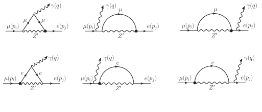
Figure 1: Feynman diagrams contributing to the $\mu\to e\gamma$ decay.

According to the definition of decay width [6], we obtain the branching ratio for the process in question

$$\textup{Br}(\mu\to e\gamma) = \frac{\alpha g_{2}^{2}}{4096\pi^{4}}\bigg{[}|F_{1}(Q_{L}^{e}-Q_{R}^{e})+F_{2}Q_{L}^{e}|^{2}|\Omega_{L\mu e}|^{2}$$ (11)

$$+|F_{1}(Q_{R}^{e}-Q_{L}^{e})+F_{2}Q_{R}^{e}|^{2}|\Omega_{R\mu e}|^{2}\bigg{]}\frac{m_{\mu}}{\Gamma_{\mu}},$$

where $\Gamma_{\mu}$ is the total decay width of the muon lepton.

III.2 The $\mu-e$ conversion process

The $\mu-e$ conversion process refers to the capture of a muon by a heavy nucleus, in which the lepton flavor conservation is not preserved [32, 33, 34]. Such processes is represented by

$$\mu^{-}+N\to e^{-}+N,$$ (12)

where the nucleus $N$ has mass and atomic number $A$ and $Z$, respectively.

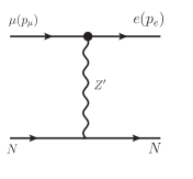
Figure 2: Feynman diagram contributing to the $\mu-e$ conversion process, non-photonic case.

In order to obtain a useful branching ratio for this process, we focus on the case of neutral current interactions with flavor violation at the tree level mediated by a $Z^{\prime}$ gauge boson (see Fig. 2). Specifically, we analyze the non-photonic process described the lepton-quark effective Lagrangian [35, 34]

$$\mathcal{L}_{eff}=\sqrt{2}\,G\,\bar{u}(p_{e})\gamma^{\lambda}\big{(}g_{V}^{\prime}-g_{A}^{\prime}\gamma_{5}\big{)}u(p_{\mu})\sum_{q=u,d,s..}\bar{q}\gamma_{\lambda}\bigg{(}v_{q}^{\prime}-a_{q}^{\prime}\gamma_{5}\bigg{)}q,$$ (13)

with the various parameters defined as

$$G =\frac{g_{2}}{\sqrt{32}m_{Z^{\prime}}^{2}},$$

$$g_{V}^{\prime} =\Omega_{L\mu e}+\Omega_{R\mu e},\,g_{A}^{\prime}=\Omega_{R\mu e}-\Omega_{L\mu e},$$

$$v_{q}^{\prime} =Q_{L}^{q_{i}}+Q_{R}^{q_{i}},\,a_{q}^{\prime}=Q_{R}^{q_{i}}-Q_{L}^{q_{i}}.$$ (14)

After algebraic manipulations and introducing the nucleon spinor $\psi_{N}=(^{p}_{n})$ and the Pauli matrix $\tau_{3}$, Eq. (13) can be rewritten as

$$\mathcal{L}_{eff}^{N}= \sqrt{2}\,G\,\bar{u}(p_{e})\gamma^{\lambda}\big{(}g_{V}^{\prime}-g_{A}^{\prime}\gamma_{5}\big{)}u(p_{\mu})$$

$$\times\bar{\psi}_{N}\gamma_{\lambda}\big{[}(C_{1S}+C_{1V}\tau_{3})-(C_{2S}+C_{2V}\tau_{3})\gamma_{5}\big{]}\psi_{N},$$ (15)

where the couplings $C_{1S}$ and $C_{1V}$ are denoted as the isoscalar vector and the isovector vector, respectively. These parameters are given explicitly as

$$C_{1S}\equiv \frac{3}{2}\big{(}v_{u}^{\prime}+v_{d}^{\prime}\big{)},$$ (16)

$$C_{1V}\equiv \frac{1}{2}\big{(}v_{u}^{\prime}-v_{d}^{\prime}\big{)}.$$ (17)

On the other hand, in Refs. [34, 36] it has been shown that the couplings of axial quarks $C_{2S}$ and $C_{2V}$ do not contribute to the coherent nuclear charge ($Q_{W}^{\prime}$), therefore the width of the $\mu-e$conversion process does not depend on these parameters. Thus, the width can be written as

$$\Gamma=\frac{g_{2}^{2}\alpha^{3}m_{\mu}^{5}}{32\pi^{2}m_{Z^{\prime}}^{4}}\frac{Z_{eff}^{4}}{Z}|F(q)|^{2}Q_{W}^{\prime\,2}\big{(}g_{V}^{\prime\,2}+g_{A}^{\prime\,2}\big{)}.$$ (18)

The most stringent bounds for capture rate are provided by gold and titanium nuclei [6]. The branching ratio for the $\mu-e$ [32] conversion is given by

$$\mathrm{Br}(\mu^{-}+N\to e^{-}+N)\equiv\frac{\Gamma(\mu^{-}+N\to e^{-}+N)}{\Gamma_{caputure}},$$ (19)

where $\Gamma_{caputure}\equiv\Gamma(\mu^{-}+N\to capture)$ is the muon decay width. For our propose of bounding the $\Omega_{R,L{\mu e}}$ couplings, we use the branching ratio for the $\mu-e$ conversion, which, according to Eq. (18), can be expressed as

$$\mathrm{Br}(\mu^{-}+N\to e^{-}+N)=\frac{g_{2}^{2}\alpha^{3}m_{\mu}^{5}}{16\pi^{2}m_{Z^{\prime}}^{4}}\frac{Z_{eff}^{4}}{Z}|F(q)|^{2}\big{(}|\Omega_{L\mu e}|^{2}+|\Omega_{R\mu e}|^{2}\big{)}\frac{Q_{W}^{\prime 2}}{\Gamma_{capture}},$$ (20)

with

$$Q_{W}^{\prime 2}=(2Z+N)(Q_{L}^{u}+Q_{R}^{u})+(Z+2N)(Q_{L}^{d}+Q_{R}^{d}).$$ (21)

We consider the $Z^{\prime}$ gauge boson for the different models aforementioned. However, as it can be appreciated from Eqs. (20) and (21), the resulting branching ratio is proportional to the quiral charges of the quarks $u$ and $d$, which vanishes for the $Z_{\chi},Z_{\psi}$ and $Z_{\eta}$ bosons, since $Q_{L}^{q}+Q_{R}^{q}=0$ [8, 37]. For the remaining bosons, $Z_{S}$ and $Z_{LR}$, we take the following parameters of the titanium nucleus: $Z_{eff}\simeq 17.6$, $F(q^{2}\simeq-m_{\mu}^{2})\simeq 0.54$ and $\Gamma_{capture}=(2.59\pm 0.012)\times 10^{-6}s^{-1}$ [35, 38, 36, 39], while the experimental bound for $\mathrm{Br}(\mu^{-}+N\to e^{-}+N)_{\mathrm{exp}}<4.3\times 10^{-12}$ [40]. Eqs. (11) and (20) will be our starting point in next subsection to constrain the $\Omega_{R,L\mu e}$ couplings.

III.3 The $\mu\to ee^{+}e^{-}$ decay

The $\mu\to ee^{+}e^{-}$ process can be directly calculated at the tree level. The corresponding Feynman diagram is shown in Fig. 3.

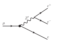
Figure 3: Feynman diagram for the $\mu\to ee^{+}e^{-}$ decay process.

By following Ref. [19], we found that Br($\mu\to ee^{+}e^{-}$) can be written as

$$\mathrm{Br}(\mu\to ee^{+}e^{-})= \frac{g_{2}^{2}}{384\pi^{3}}\left[f(\frac{m_{Z^{\prime}}^{2}}{m_{\mu}^{2}})\left(|Q_{L}^{e}\Omega_{L\mu e}|^{2}+|Q_{R}^{e}\Omega_{R\mu e}|^{2}\right)\right.$$

$$\left.+h(\frac{m_{Z^{\prime}}^{2}}{m_{\mu}^{2}})\left(|Q_{L}^{e}\Omega_{R\mu e}|^{2}+|Q_{R}^{e}\Omega_{L\mu e}|^{2}\right)\right]\frac{m_{\mu}}{\Gamma_{\mu}},$$ (22)

where

$$f(a)= \int_{0}^{1}dx\frac{2x-1}{(x-1+a)^{2}}(2(7-4x)x-5)\approx\frac{1}{a},$$

$$h(a)= \int_{0}^{1}dx\frac{2x-1}{(x-1+a)^{2}}(1-2(x-1)x)\approx\frac{1}{a^{2}}.$$

In last equations, our approximations are valid for $a=\frac{m_{Z^{\prime}}^{2}}{m_{\mu}^{2}}>>1$, which stand for $m_{Z^{\prime}}>$ 1 TeV. Thus, the function $h(a)$ is suppressed with respect to the function $f(a)$ by at lest 8 orders of magnitude. So, we can can drop the term, $h(\frac{m_{Z^{\prime}}^{2}}{m_{\mu}^{2}})\left(|Q_{L}^{e}\Omega_{R\mu e}|^{2}+|Q_{R}^{e}\Omega_{L\mu e}|^{2}\right)$ in (22) and this simplifies the bounding process of the couplings. In this manner the final expression for the branching ratio is expressed as

$$\mathrm{Br}(\mu\to ee^{+}e^{-})\approx\frac{g_{2}^{2}}{384\pi^{3}}f(\frac{m_{Z^{\prime}}^{2}}{m_{\mu}^{2}})\left(|Q_{L}^{e}\Omega_{L\mu e}|^{2}+|Q_{R}^{e}\Omega_{R\mu e}|^{2}\right)\frac{m_{\mu}}{\Gamma_{\mu}}.$$ (23)

III.4 Bounding the $\Omega_{\mu e}$ coupling

As it was mentioned, we are interested in bounding the flavor-violating branching ratio of the $Z^{\prime}$ gauge boson decaying into the $\mu$ and $e$ leptons. In order to do that, we firstly bound the $|\Omega_{R,L\mu e}|^{2}$ couplings by using the branching ratios in Eqs. (11), (20) and (23). The task is carried out by considering each of the previous results as follows.

III.4.1 By using the $\mu\to e\gamma$ process

To numerically constrain the couplings, we use Eq. (11) along with the experimental bound: Br$(\mu\to e\gamma)_{\tiny\mathrm{Exp}}<4.2\times 10^{-13}$ with 90% C.L [6]. Also, we take the following experimental values of the masses of the particles involved: $m_{\mu}=0.105658$ GeV and $m_{e}=0.00051099$ GeV. In addition, we use the most recent experimental limits established for the mass of the various $Z^{\prime}$ gauge bosons, which, most of them, are larger than 3.9 TeV [17, 18]. However, the mass of $Z_{LR}$ boson predicted by the left-right symmetric model is larger than 1.162 TeV [41]. In this way, in next section we propose an analysis for the couplings between 2 and 7 TeV for $m_{Z^{\prime}}$. For the study, we consider three different cases:

a) Vector-like coupling. For this case, we have that $\Omega_{L\mu e}=\Omega_{R\mu e}\equiv\Omega_{\mu e}$. Therefore, the bound can be expressed as

$$|\Omega_{\mu e}|^{2}< \frac{4096\pi^{4}}{\alpha}\frac{\Gamma_{\mu}}{m_{\mu}}\frac{4.2\times 10^{-13}}{g_{2}^{2}\big{[}|F_{1}(Q_{L}^{e}-Q_{R}^{e})+F_{2}Q_{L}^{e}|^{2}+|F_{1}(Q_{R}^{e}-Q_{L}^{e})+F_{2}Q_{R}^{e}|^{2}\big{]}},$$ (24)

where we have taken the lower bound of Br$(\mu\to e\gamma)_{\tiny\mathrm{exp}}$ in accordance to Eq.(11). In Fig. 4 (a) it is shown the maxima values of $|\Omega_{\mu e}|^{2}$ as a function of $m_{Z^{\prime}}$ for the different models. As it can be observed, the most restrictive bound corresponds to the $Z_{\chi}$ boson, while the less restrictive corresponds to the $Z_{\eta}$ boson, along the mass interval studied.

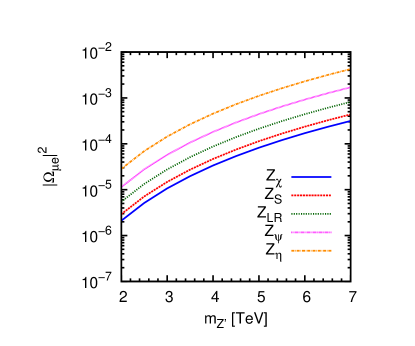
(a)

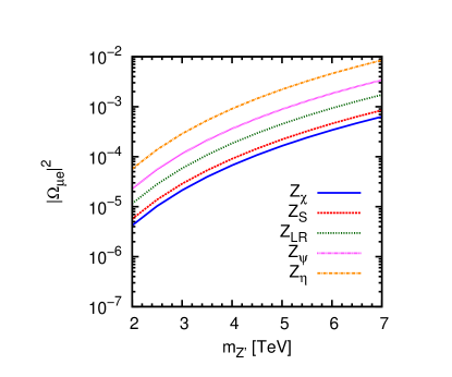
(b)

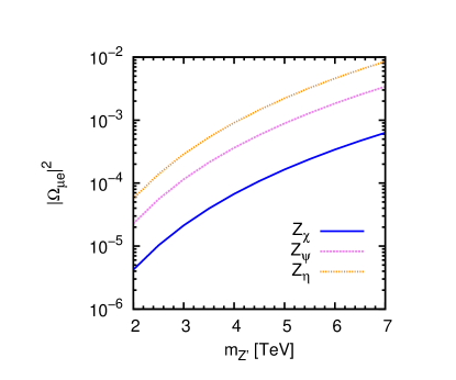
(c)

Figure 4: Bounds for the $Z^{\prime}\mu e$ coupling as a function of $m_{Z^{\prime}}$, obtained through the $\mu\to e\gamma$ decay. In (a), vector-like coupling case. In (b), maximal parity violation case. In (c), the complete case.

b) Maximal parity violation. For this case, we take $\Omega_{L\mu e}=0$. Thus the corresponding bounding can be written as

$$|\Omega_{R\mu e}|^{2}< \frac{4096\pi^{4}}{\alpha}\frac{\Gamma_{\mu}}{m_{\mu}}\frac{4.2\times 10^{-13}}{g_{2}^{2}\big{[}|F_{1}(Q_{L}^{e}-Q_{R}^{e})+F_{2}Q_{R}^{e}|^{2}\big{]}}.$$ (25)

In Fig. 4 (b) it can be appreciated the behavior of maxima of $|\Omega_{R\mu e}|^{2}$ as function of $m_{Z^{\prime}}$ for the different models under consideration. As before, the most restrictive case corresponds precisely to the $Z_{\chi}$ boson, and the less restrictive case is for the $Z_{\eta}$ boson.

c) Complete case. This particular case is only achieved for the three different models that share the same absolute value of the left and right chiral charges $|Q_{L}^{e}|=|Q_{R}^{e}|$, namely, the $Z_{\chi},Z_{\psi}$ and $Z_{\eta}$ bosons. For this case, we have

$$|\Omega_{L\mu e}|^{2}+|\Omega_{R\mu e}|^{2}< \frac{4096\pi^{4}}{\alpha}\frac{\Gamma_{\mu}}{m_{\mu}}\frac{4.2\times 10^{-13}}{g_{2}^{2}|2F_{1}+F_{2}|^{2}|Q_{L}^{e}|^{2}}.$$ (26)

The maxima values allowed for the sum $|\Omega_{L\mu e}|^{2}+|\Omega_{R\mu e}|^{2}$ are depicted in Fig. 4 (c). As it can be observed, the most restrictive bound is achieved by the $Z_{\chi}$ boson.

Finally, let us mention that the resulting growing behavior of square magnitude of the couplings in the mass interval under analysis is consistent with the perturbative regime employed to carry out the study of the $Z^{\prime}$ boson decay.

III.4.2 By using the $\mu-e$ conversion process

Let us now use the $\mu-e$ conversion branching ratio in Eq. (20) to analyze the behavior of the couplings. For the study, we consider the same three cases above discussed:

a) The vector-like coupling. For this case: $\Omega_{L\mu e}=\Omega_{R\mu e}\equiv\Omega_{\mu e}$. Therefore,

$$|\Omega_{\mu e}|^{2}<\mathrm{Br}(\mu^{-}+N\to e^{-}+N)_{\mathrm{exp}}\>\frac{8\pi^{2}\,m_{Z^{\prime}}^{4}\,Z\,\Gamma_{capture}}{g_{2}^{2}\alpha^{3}\,m_{\mu}^{5}Z_{eff}^{4}|F(q)|^{2}Q_{W}^{{}^{\prime}2}}.$$ (27)

b) The coupling with maximal parity violation. For this case $\Omega_{L\mu e}=0$. Thus

$$|\Omega_{R\mu e}|^{2}<\mathrm{Br}(\mu^{-}+N\to e^{-}+N)_{\mathrm{exp}}\>\frac{16\pi^{2}\,m_{Z^{\prime}}^{4}\,Z\,\Gamma_{capture}}{g_{2}^{2}\alpha^{3}\,m_{\mu}^{5}Z_{eff}^{4}|F(q)|^{2}Q_{W}^{{}^{\prime}2}}.$$ (28)

c) Complete case. Here, the parameter under consideration is $|\Omega_{L\mu e}|^{2}+|\Omega_{R\mu e}|^{2}$. However, this case is the same as to the previous one, since it has the same expression in the right hand of the inequality in (28).

In Figs. 5 (a) and (b), the upper bounds of the couplings in question as a function of $m_{Z^{\prime}}$ are shown. As it can be observed in these figures, the most restrictive bounds are provided by the $Z_{LR}$ boson and they result less than $10^{-6}$ almost along the full mass interval.

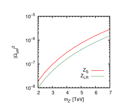
(a)

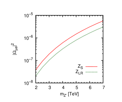
(b)

Figure 5: Bounds for the $|\Omega_{\mu e}|^{2}$ parameter as function of $m_{Z^{\prime}}$ obtained through the $\mu-e$ conversion process. (a) For the case of vector-like coupling. (b) Maximal parity violation coupling and complete cases.

III.4.3 By using the $\mu\to ee^{+}e^{-}$ decay

Once again, we consider the three cases previously discussed. To accomplish the task of bounding the couplings, we use Eq. (23) along with the experimental bound $\mathrm{Br}(\mu\to ee^{+}e^{-})_{\mathrm{exp}}<1.0\times 10^{-12}$ [6]. The corresponding results are listed below.

a) Vector-like coupling: The corresponding bound is

$$|\Omega_{\mu e}|^{2}<384\pi^{3}\frac{\Gamma_{\mu}}{m_{\mu}}\frac{\mathrm{Br}(\mu\to ee^{+}e^{-})_{\mathrm{exp}}}{\big{[}g_{2}^{2}({Q_{L}^{e}}^{2}+{Q_{R}^{e}}^{2})\big{]}f(\frac{m_{Z^{\prime}}^{2}}{m_{\mu}^{2}})}.$$ (29)

b) Maximal parity violation coupling:

$$|\Omega_{R\mu e}|^{2}<384\pi^{3}\frac{\Gamma_{\mu}}{m_{\mu}}\frac{\mathrm{Br}(\mu\to ee^{+}e^{-})_{\mathrm{exp}}}{g_{2}^{2}{Q_{R}^{e}}^{2}f(\frac{m_{Z^{\prime}}^{2}}{m_{\mu}^{2}})}.$$ (30)

c) Complete case:

$$|\Omega_{L\mu e}|^{2}+|\Omega_{R\mu e}|^{2}<384\pi^{3}\frac{\Gamma_{\mu}}{m_{\mu}}\frac{\mathrm{Br}(\mu\to ee^{+}e^{-})_{\mathrm{exp}}}{g_{2}^{2}{Q_{L}^{e}}^{2}f(\frac{m_{Z^{\prime}}^{2}}{m_{\mu}^{2}})}.$$ (31)

In Fig. 6, it is shown the behavior of bounds in question. As it can be observed, the most restrictive bounds for the couplings come from the $Z_{\chi}$ boson in the three cases. On the contrary, the less restrictive bounds are provided by the $Z_{\eta}$ boson. In general, the case of vector-like coupling offers the most restrictive bounds. Although, as the bounds arising from the $Z_{S}$ and $Z_{LR}$ gauge bosons are concerned, the most restrictive ones result from the $\mu-e$ conversion process, as it can be appreciated from Figs. 5 (a) and 6 (a).

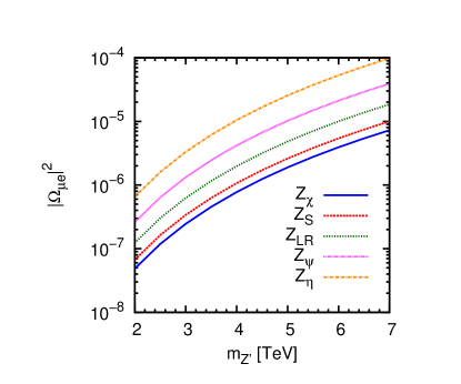
(a)

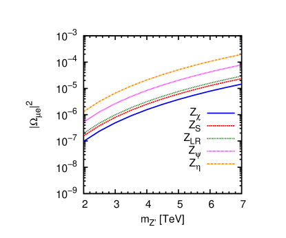
(b)

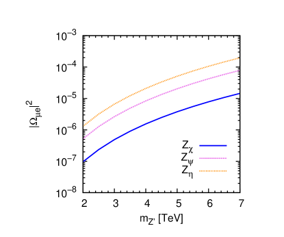
(c)

Figure 6: Bounds for the $|\Omega_{\mu e}|^{2}$ parameter as function of $m_{Z^{\prime}}$ obtained through the $\mu\to ee^{+}e^{-}$ decay. In (a), vector-like coupling case. In (b), maximal parity violation case. In (c), the complete case.

IV The $Z^{\prime}\to\mu e$ decay

The Feynman rules for this process can be obtained from the Lagrangian in (7). By following the usual procedures, we obtain that the general branching ratio for the lepton flavor violating process $Z^{\prime}\to l_{i}l_{j}$ can be written as

$$\textup{Br}(Z^{\prime}\to l_{i}l_{j})\approx\frac{m_{Z^{\prime}}}{12\pi\,\Gamma_{Z^{\prime}}}\bigg{(}|\Omega_{Ll_{i}l_{j}}|^{2}+|\Omega_{Rl_{i}l_{j}}|^{2}\bigg{)},$$ (32)

where $\Gamma_{Z^{\prime}}$ is the total decay width of the $Z^{\prime}$ boson, and it was considered that $m_{\mu}/m_{Z^{\prime}}\ll 1$. On account of $\Gamma_{Z^{\prime}}$, we consider all possible decay modes that include both flavor-conserving and flavor-violating decays [19, 15, 42], that is to say, the decay of $Z^{\prime}$ to $\nu_{e}\bar{\nu_{e}},\nu_{\mu}\bar{\nu_{\mu}},\nu_{\tau}\bar{\nu_{\tau}},e\bar{e},\mu\bar{\mu},\tau\bar{\tau},u\bar{u},c\bar{c},t\bar{t},d\bar{d},s\bar{s},b\bar{b},\bar{u}c+u\bar{c},\bar{t}c+t\bar{c},\bar{\tau}\mu+\tau\bar{\mu},\bar{\tau}e+\tau\bar{e}$, and $\bar{\mu}e+\bar{e}\mu$. Notice that the total decay width $\Gamma_{Z^{\prime}}$ is model dependent, since each decay mode of this particle is also model dependent. Previously, we have analyzed three different cases to bounding the couplings, through the three process above discussed, which will be used in the numerical analysis of the $Z^{\prime}\to\mu e$ decay. For the discussion, we restrict ourselves to the vector-like coupling case, which gives the most restrictive bounds for the decay in question. As matter of fact, the others cases provide bounds of the same order of magnitude for each $m_{Z^{\prime}}$, along the mass interval. Due to the values of the chiral charges (which make the branching ratio in (32) a non-trivial function of these charges), and the $\Omega$ couplings, the bounds for the branching ratio can change up to three orders of magnitude, as it is discussed below.

In Fig. 7 (a) it is shown the bounds of the branching ratio for the $Z^{\prime}\to\mu e$ decay, calculated by using the $\mu\to e\gamma$ decay. As we can see, the $Z_{\eta}$ boson provides the less restrictive bound for the decay, with values less than $10^{-4}$ almost over the entire interval [2,7] TeV. The most suppressed bound corresponds to the $Z_{S}$ boson, which gives values for $\mathrm{Br}(Z^{\prime}\to\mu e)<10^{-5}$ for masses below 5 TeV, reaching the value of $1.32\times 10^{-4}$ at $m_{Z^{\prime}}=$ 7 TeV. For the rest of the models, the corresponding branching ratios vary between $10^{-5}$ and $10^{-4}$.

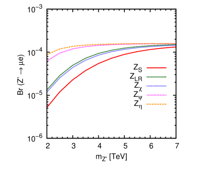
(a)

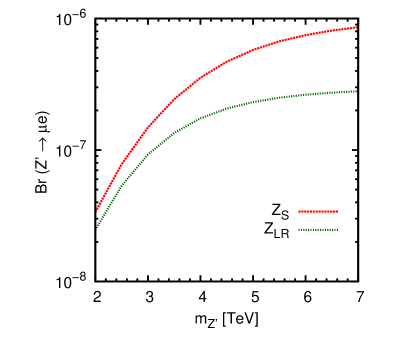
(b)

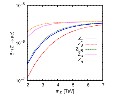
(c)

Figure 7: The branching ratios for the LFV decay of $Z^{\prime}\to\mu e$ as a function of $m_{Z^{\prime}}$. The branching ratio was obtained by means of: (a) The $\mu\to e\gamma$ decay. (b) The $\mu-e$ conversion process in nuclei. (c) The $\mu\to ee^{+}e^{-}$ decay.

Let us now discuss the results of bounds for the branching ratio by using the predictions for the $\Omega_{\mu e}$ coupling coming from the $\mu-e$ conversion process. In Fig. 7 (b), the behavior of such bounds is shown as a function of $m_{Z^{\prime}}$. As it can be observed, the resulting bounds for the $Z_{S}$ and $Z_{LR}$ bosons are more restrictive than the corresponding ones obtained through the $\mu\to e\gamma$ decay (shown in Fig. 7 (a)), since the less restrictive result for the branching ratio is $<10^{-6}$, even in the most conservative scenario, which is obtained with the $Z_{S}$ boson.

As far as the bounds for $\mathrm{Br}(Z^{\prime}\to\mu e)$ resulting from the $\mu\to ee^{+}e^{-}$ decay is concerned, the results are shown in Fig. 7 (c). The numerical values for the bounds show that the corresponding branching ratios are more suppressed than the obtained through the $\mu\to e\gamma$ decay by two order of magnitude for each $Z^{\prime}$ boson. Nevertheless, the only non-vanishing branching ratios (for $Z_{S}$ and $Z_{LR}$ bosons), obtained by means of the $\mu-e$ conversion process, result more suppressed along the mass interval analyzed than the obtained by using the $\mu\to e\gamma$ decay or the $\mu\to ee^{+}e^{-}$ decay.

Complementarily, we also present contour plots for the Br$(Z^{\prime}\to\mu e)$ as function of $m_{Z\prime}$ and $|\Omega|^{2}$ (see Figs. 8, 9 and 10) only for the vector-like case, since it provides the most stringent predictions. In these plots (one for each model and bounding approach) it is shown the excluded regions for specific branching ratios.

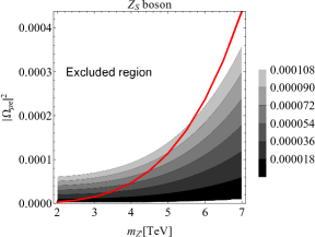
(a)

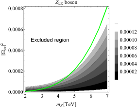
(b)

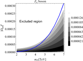
(c)

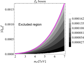
(d)

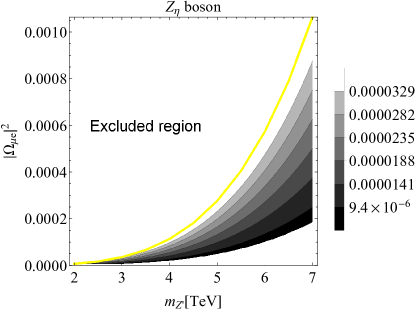
(e)

Figure 8: Contour plots for the Br$(Z^{\prime}\to\mu e)$. The graphs were obtained by using the $\mu\to e\gamma$ decay process. In (a) for the $Z_{S}$ boson, in (b) for the $Z_{LR}$ boson, in (c) for the $Z_{\chi}$ boson, in (d) for the $Z_{\psi}$ boson, and in (e) for the $Z_{\eta}$ boson. In all the cases the thick line in color separates the excluded from the allowed region.

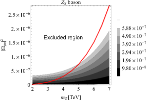
(a)

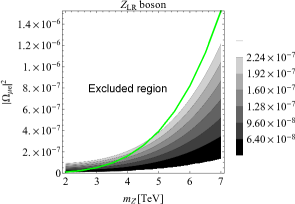
(b)

Figure 9: Contour plots for the Br$(Z^{\prime}\to\mu e)$. The graphs were obtained by using the $\mu-e$ conversion process. In (a) for the $Z_{S}$ boson and in (b) for the $Z_{LR}$ boson. In both cases the thick line in color separates the excluded from the allowed region.

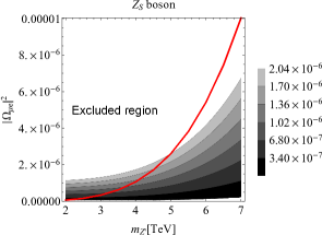
(a)

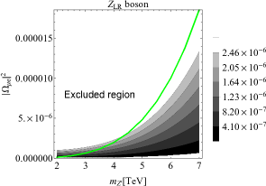
(b)

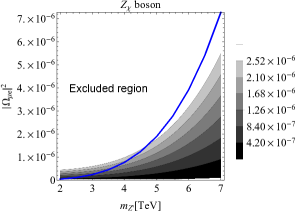
(c)

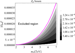
(d)

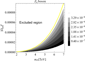
(e)

Figure 10: Contour plots for the Br$(Z^{\prime}\to\mu e)$. The graphs were obtained by using the $\mu\to ee^{+}e^{-}$ decay process. In (a) for the $Z_{S}$ boson, in (b) for the $Z_{LR}$ boson, in (c) for the $Z_{\chi}$ boson, in (d) for the $Z_{\psi}$ boson, and in (e) for the $Z_{\eta}$ boson. In all the cases the thick line in color separates the excluded from the allowed region.

V Conclusions

The $Z^{\prime}$ gauge boson is proposed in several extensions of the SM that induces FCNC at the tree level. This particle is under quest by the CMS and ATLAS experimental groups at LHC who have established experimental bounds on its mass. The existence of this particle could explain physical processes, such as the flavor-violating decays in the sector of leptons that are very suppressed in the SM, whose numerical values are not compatible with the respective experimental results. In this work, we have studied the flavor-violating branching ratio of decay of the $Z^{\prime}$ gauge boson into $\mu e$ leptons, using different extended models and three different ways of bounding the decay. By resorting to the $\mu\to e\gamma$ process, we found bounds for the $\mathrm{Br}(Z^{\prime}\to\mu e)$ as function of $m_{Z^{\prime}}$; depending on the model, the values go from $10^{-6}$ to $10^{-4}$, along the mass interval analyzed. If instead, the $\mu-e$ conversion process is used, we obtain more restrictive bounds for the branching ratio of the $Z^{\prime}\to\mu e$ decay. In specific, the values of the branching ratio go from $10^{-8}$ to $10^{-6}$. However, due to the property $Q_{L}^{q}+Q_{R}^{q}=0$ of the chiral charges of quarks the only non-vanishing branching ratios for this process correspond to the $Z_{S}$ and $Z_{LR}$ bosons. For the case of the tree-body decay: $\mu\to ee^{+}e^{-}$, the resulting bounds for $\mathrm{Br}(Z^{\prime}\to\mu e)$ are more suppressed than the obtained in the cases above discussed, except for that related to the $Z_{S}$ and $Z_{LR}$ bosons. In fact, in this case the bounds of the branching ratio go from $10^{-7}$ to $10^{-6}$. If we compare these bounds with the current experimental bound for the SM decay $\mathrm{Br}(Z\to\mu e)<7.5\times 10^{-7}$, the bounds for the $\mathrm{Br}(Z^{\prime}\to\mu e)$ result less restrictive or at least comparable.

Appendix

Form Factors:

$$F_{1} = 6+x_{\mu}^{2}+\frac{3(3x_{\mu}^{2}-1)}{x_{\mu}^{2}(x_{\mu}^{2}-1)}\textup{Log}(x_{\mu}^{2})+6\frac{\big{(}1-4x_{\mu}^{2}\big{)}^{1/2}}{x_{\mu}^{2}}\textup{Log}\bigg{(}\frac{1+\big{(}1-4x_{\mu}^{2}\big{)}^{1/2}}{2x_{\mu}}\bigg{)},$$

$$F_{2} = 8+2\Bigg{[}-\frac{4}{x_{\mu}^{2}}-\frac{3x_{\mu}^{2}-1}{x_{\mu}^{4}(x_{\mu}^{2}-1)}\textup{Log}(x_{\mu}^{2})+\textup{Log}\bigg{(}\frac{1+\big{(}1-4x_{\mu}^{2}\big{)}^{1/2}}{2}\bigg{)}^{2}$$

$$+ 2\bigg{[}\bigg{(}\frac{x_{\mu}^{2}-1}{x_{\mu}^{2}}\bigg{)}^{2}\textup{Log}\bigg{(}\frac{1}{1-x_{\mu}^{2}}\bigg{)}-\frac{\big{(}1-4x_{\mu}^{2}\big{)}^{1/2}}{x_{\mu}^{4}}\textup{Log}\bigg{(}\frac{1+\big{(}1-4x_{\mu}^{2}\big{)}^{1/2}}{2x_{\mu}}\bigg{)}$$

$$+ \textup{Polylog}\bigg{(}2,1-\frac{1}{x_{\mu}^{2}}\bigg{)}+\textup{Polylog}\bigg{(}2,\frac{2x_{\mu}^{2}}{1+\big{(}1-4x_{\mu}^{2}\big{)}^{1/2}}\bigg{)}$$

$$- \textup{Polylog}\bigg{(}2,\frac{2x_{\mu}^{2}}{-1+2x_{\mu}^{2}+\big{(}1-4x_{\mu}^{2}\big{)}^{1/2}}\bigg{)}\bigg{]}\Bigg{]},$$

where $x_{\mu}=\frac{m_{\mu}}{m_{Z^{\prime}}}$.

References

- [1] For instance, see G. Eilam, J. L. Hewett, and A. Soni, Phys. Rev. D 44, 1473 (1991); 59, 039901(E) (1998); N. G. Deshpande, B. Margolis, and H. D. Trottier, Phys. Rev. D 45, 178 (1992); B. Mele, S. Petrarca, and A Soddu, Phys. Lett. B 435, 401 (1998); A. Cordero-Cid, J. M. Hernández, G. Tavares-Velasco, and J. J. Toscano, Phys. Rev. D 73, 094005 (2006); G. Eilam, M. Frank, and I. Turan, Phys. Rev. D 73, 053011 (2006); 74, 035012 (2006), M. Artuso et al, Eur. Phys. J. C 57, 309-492 (2008).
- [2] R. Becker-Szendy, C. B. Bratton, D. Casper, S. T. Dye, W. Gajewski, M. Goldhaber et al., Phys. Rev. D 46, 3720 (1992); Y. Fukuda et al., Phys. Lett. B335, 237 (1994); Phys. Rev. Lett. 81, 1562 (1998); H. Sobel, Nucl. Phys. B, Proc. Suppl. 91, 127 (2001); M. Ambrossio et al., Phys. Lett. B566, 35 (2003); Y. Ashie et al., Phys. Rev. D 71, 112005 (2005); W. W. M. Allison, G. J. Alner, D. S. Ayres, G. D. Barr, W. L. Barrett, P. M. Border, et al., Phys. Rev. D 72, 052005 (2005); P. Adamson et al., Phys. Rev. D 73, 072002 (2006).
- [3] M. Apollonio et al., Eur. Phys. J. C 27, 331 (2003); S. N. Ahmed et al., Phys. Rev. Lett. 92, 181301 (2004); M. B. Smy et al., Phys. Rev. D 69, 011104 (2004); E. Aliu et al., Phys. Rev. Lett. 94, 081802 (2005).
- [4] Y. Fukuda, et al., Phys. Rev. Lett. 82, 2644 (1999); Q. R. Ahmad, et al., Phys. Rev. Lett. 89, 011301 (2002); K. Eguchi, et al., Phys. Rev. Lett. 90, 021802 (2003).
- [5] T-P Cheng, L-F Li, Gauge Theory of Elementary Particle Physics, Clarendon Press, Oxford (1984).
- [6] R.L. Workman et al. (Particle Data Group), Prog. Theor. Exp. Phys. 2022, 083C01 (2022).
- [7] A. Méndez, Ll. M. Mir, Phys. Rev. D 40, 251 (1989); S. Nussinov, R. D. Peccei,and X. M. Zhang, Phys. Rev. D 63, 016003 (2000); D, Delépine and F. Vissani, Phys. Lett. B522, 95 (2001); E. O. Iltan and I. Turan, Phys. Rev. D 65, 013001 (2001); A. Flores-Tlalpa, J. M. Hernández, G. Tavares-Velasco, and J. J. Toscano, Phys. Rev. D 65, 073010 (2002); M. A. Perez, G. Tavares-Velasco, and J. J. Toscano, Int. J. Mod. Phys. A 19, 159 (2004); L. Calibbi, X. Marcano, and J. Roy, Eur. Phys. J. C 81, 1054 (2021).
- [8] R. W. Robinett and J. L. Rosner, Phys. Rev. D 26, 2396 (1982); R. W. Robinett, Phys. Rev. D26, 2388 (1982).
- [9] P. Langacker and M. Luo, Phys. Rev. D 45, 278 (1992).
- [10] F. Zwirner, Int. J. Mod. Phys. A3, 49 (1988).
- [11] J.L. Hewett and T.G. Rizzo, Phys. Rep. 183, 193 (1989).
- [12] M. A. Perez and M. A. Soriano, Phys. Rev. D 46, 284 (1992).
- [13] P.H. Frampton, Phys. Rev. Lett. 69, 2889 (1992).
- [14] A. Leike, Phys. Rept. 317, 143 (1999).
- [15] A. Arhrib, K. Cheung, C-W Chiang, and T-C Yuan, Phys. Rev. D 73, 075015 (2006).
- [16] Paul Langacker, Rev. Mod. Phys. 81, 1199 (2009).
- [17] M. Aaboud et al. (ATLAS Collaboration), Phys. Lett. B761, 372 (2016);
- [18] A. M. Sirunyan et al. (CMS Collaboration), JHEP 06, 120 (2018).
- [19] J. I. Aranda, J. Montaño, F. Ramírez-Zavaleta, J. J. Toscano, and E. S. Tututi, Phys. Rev. D 86, 035008 (2012).
- [20] The CMS Collaboration, arXiv:2205.06709; JHEP 04, 073 (2018).
- [21] M. Aaboud et al. (ATLAS Collaboration), Phys. Rev. D 98, 092008 (2018).
- [22] Hiren H. Patel, Comput. Phys. Commun. 197, 276 (2015).
- [23] G.-C Cho, K. Hagiwara and Y. Umeda, Nucl. Phys. B531, 65 (1998).
- [24] P. Langacker and J. Wang, Phys. Rev. D 58, 115010 (1998).
- [25] L. S. Durkin and P. Langacker, Phys. Lett. B166, 436 (1986); M. Cvetic and P. Langacker, Proceedings of Ottawa 1992: Beyond the standard model 3, 454-458, (1992); C-W Chiang, Yi-Fan Lin, and Jusak Tandean, JHEP 11, 083 (2011).
- [26] R. W. Robinett, J. L. Rosner, Phys. Rev. D 25, 3026 (1982); Erratum Phys. Rev. D 27, 679 (1983).
- [27] P. Langacker and M. Plümacher, Phys. Rev. D 62, 013006 (2000); X.-G. He and G. Valencia, Phys. Rev. D 74, 013011 (2006); C.-W. Chiang, N. G. Deshpande, and J. Jiang, JHEP 08, 075 (2006).
- [28] M. Cveti, B. Kayser and P. Langacker, Phys. Rev. Lett. 68, 2871 (1992).
- [29] F. del Aguila, Acta Phys. Pol. B 25, 1317 (1994); arXiv: hep-ph/9404323.
- [30] J. C. Pati and A. Salam, Phys. Rev. D 10, 275 (1974); Erratum Phys. Rev. D 11, 703 (1975);
- [31] J. I. Aranda, E. Cruz-Albaro, D. Espinosa-Gómez, J. Montaño, F. Ramírez-Zavaleta, and E. S. Tututi, Int. J. Mod. Phys. A36, 2150167 (2021).
- [32] Y. Kuno and Y. Okada, Rev. Mod. Phys. 73, 151 (2001).
- [33] A. Faessler, T. Gutsche, S. Kovalenko, V. E. Lyubovitskij, and I. Schmidt, Phys. Rev. D 72, 075006 (2005).
- [34] T. S. Kosmas, G. K. Leontaris, and J. D. Vergados, Prog. Part. Nucl. Phys. 33, 397 (1994).
- [35] J. Bernabéu, E. Nardi and D. Tommasini, Nucl. Phys. B 409, 69 (1993).
- [36] H. C. Chiang, E. Oset, T. S. Kosmas, A. Faessler and J. D. Vergados, Nucl. Phys. A 559, 526 (1993).
- [37] J. Montaño-Domínguez, B. Quezadas-Vivian, F. Ramírez-Zavaleta, and E.S. Tututi, J. Phys. G 49, 075004 (2022).
- [38] T. Suzuki, D.F. Measday, and J.P. Roalsvig, Phys. Rev. C 35, 2212 (1987).
- [39] H. C. Chiang, E. Oset and P. Fernández de Córdoba, Nucl. Phys. A 510, 591 (1990).
- [40] C. Dohmen, et al, SUNDRUM II Collab. Phys. Lett. B 317, 631 (1993).
- [41] F. del Aguila, J. de Blas, and M. Perez-Victoria, JHEP 09, 033 (2010), arXiv:1005.3998.
- [42] J. I. Aranda, F. Ramírez-Zavaleta, J. J. Toscano, and E. S. Tututi, J. Phys. G: Nucl. Part. Phys. 38, 045006 (2011).