HaloFlow I: Neural Inference of Halo Mass from Galaxy Photometry and Morphology

Abstract

We present HaloFlow, a new machine learning approach for inferring the mass of host dark matter halos, $M_{h}$, from the photometry and morphology of galaxies. HaloFlow uses simulation-based inference with normalizing flows to conduct rigorous Bayesian inference. It is trained on state-of-the-art synthetic galaxy images from Bottrell et al. (2023) that are constructed from the IllustrisTNG hydrodynamic simulation and include realistic effects of the Hyper Suprime-Cam Subaru Strategy Program (HSC-SSP) observations. We design HaloFlow to infer $M_{h}$ and stellar mass, $M_{*}$, using $grizy$ band magnitudes, morphological properties quantifying characteristic size, concentration, and asymmetry, total measured satellite luminosity, and number of satellites. We demonstrate that HaloFlow infers accurate and unbiased posteriors of $M_{h}$. Furthermore, we quantify the full information content in the photometric observations of galaxies in constraining $M_{h}$. With magnitudes alone, we infer $M_{h}$ with $\sigma_{\log M_{h}}\sim 0.115$ and 0.182 dex for field and group galaxies. Including morphological properties significantly improves the precision of $M_{h}$ constraints, as does total satellite luminosity: $\sigma_{\log M_{h}}\sim 0.095$ and 0.132 dex. Compared to the standard approach using the stellar-to-halo mass relation, we improve $M_{h}$ constraints by $\sim$40%. In subsequent papers, we will validate and calibrate HaloFlow with galaxy-galaxy lensing measurements on real observational data.

1 Introduction

Inferring the masses of host dark matter halos of galaxies has significant implications for cosmology and galaxy formation. The abundance of most massive halos that host galaxy clusters, for instance, is sensitive to both the expansion history of the Universe and the growth rate of structure (e.g. Voit, 2005; Allen et al., 2011; Kravtsov & Borgani, 2012; Weinberg et al., 2013; Mantz et al., 2015; Dodelson et al., 2016). It was identified as one of the most promising dark energy probes by the Dark Energy Task Force (Albrecht et al., 2006). With upcoming wide-field surveys such as the Vera C. Rubin Observatory Legacy Survey of Space and Time (LSST; Ivezić et al., 2019), galaxy cluster studies are expected to significantly improve current constraints on dark energy.

Dark matter halos also profoundly influence the evolution and properties of galaxies that they host (see Wechsler & Tinker, 2018, for a recent review). Galaxy properties, such as color, stellar mass, star formation rates, and morphology, have long been shown to depend significantly on local environment, which is primarily defined by the halo (e.g. Oemler, 1974; Davis & Geller, 1976; Dressler, 1980; Hogg et al., 2004; Kauffmann et al., 2004; Blanton et al., 2005; Baldry et al., 2006; Blanton & Moustakas, 2009; Hahn et al., 2015). Observational studies of this galaxy-halo connection have now firmly established that halo mass plays the most dominant role (e.g. Tinker et al., 2011; Moster et al., 2018; Behroozi et al., 2019).

Halos can also be used to investigate the cosmic baryon distribution. They harbor a significant fraction of cosmic baryons, both in their stellar and interstellar media (ISM) components as well as in their extended circum-galactic media (CGM). The CGM, notably, exists in a warm ionized state that is not easily amenable to direct observations. This leads to large uncertainties regarding their overall contribution to the cosmic baryon budget, i.e. part of the so-called “missing baryon problem” (e.g. Fukugita & Peebles, 2004; Cen & Ostriker, 2006; Bregman, 2007). Fast radio bursts (FRBs, see Cordes & Chatterjee 2019 for a review) are a new probe that can constrain the integrated free electron column density along each line-of-sight through their observed frequency dispersion (e.g., McQuinn, 2014; Macquart et al., 2020). By combining localized FRBs with detailed observations of intervening foreground galaxies, ongoing observations promise to constrain the cosmic baryon partition between the CGM and the intergalactic medium (IGM) (Lee et al., 2022, 2023). However, since the amount and extent of CGM gas is expected to scale with the underlying halo mass (Prochaska & Zheng, 2019; Khrykin et al., 2023), uncertainties in the halo mass of the intervening galaxies constitute a major source of uncertainty in efforts to study the cosmic baryon distribution.

Despite the pivotal role that halos play across cosmology and galaxy evolution, inferring the properties of halos remains a major observational challenge. A number of different methods are currently used to infer halo mass. For example, the gravitational potential of halos can be directly probed using gravitational lensing (e.g. Mandelbaum et al., 2006; Cacciato et al., 2009, 2013; Mandelbaum et al., 2016; Huang et al., 2020). Lensing mass measurements, however, require deep and high resolution imaging especially for lower mass halos. This makes it difficult to extend the approach to large galaxy samples. Satellite kinematics has also been used to infer halo mass (e.g. Norberg et al., 2008; More et al., 2009, 2011; Lange et al., 2019). These studies, however, rely on the assumption of virial equilibrium, velocity bias between the distribution of matter and satellite galaxies, and accurate identification of satellite galaxies. Galaxy-based halo mass estimation methods that use the phase space or richness information of galaxies, more broadly, have been shown to be significantly susceptible to systematics (see Old et al., 2014, 2015, 2018; Wojtak et al., 2018, for an overview).

There are also more indirect methods for inferring halo mass. Abundance matching methods assume a monotonic relation between halo mass and galaxy stellar mass or luminosity. Halo masses are assigned to galaxies by matching the cumulative number densities of halos and galaxies (Kravtsov et al., 2004; Tasitsiomi et al., 2004; Vale & Ostriker, 2004; Hearin et al., 2013). Such approach has also been used in conjunction with halo-based group finding algorithms: e.g. Yang et al. (2009); Tinker et al. (2011); Tinker (2022). These methods ultimately rely on the well-studied stellar-to-halo-mass relation (SHMR; see Wechsler & Tinker, 2018, and references therein). Consequently, they do not exploit additional galaxy properties beyond stellar mass: e.g. color, morphology.

In this work, we present HaloFlow, a new machine learning (ML) based approach that utilize the full photometric and morphological information of galaxies for inferring their host halo masses. HaloFlow goes beyond previous ML-based halo mass estimation methods (e.g. Ntampaka et al., 2015, 2016; Calderon & Berlind, 2019; Villanueva-Domingo et al., 2022) in two key ways. First, it uses simulation-based inference (SBI) based on neural density estimation to conduct rigorous Bayesian inference. We produce full posterior distributions of halo masses that accurately quantify the statistical uncertainties. Second, HaloFlow is designed to be applied directly to observations. To do this, we use state-of-the-art synthetic galaxy images made with a dust radiative transfer forward model (Bottrell et al., 2023). The images are constructed from the IllustrisTNG cosmological magneto-hydrodynamical simulations (hereafter “TNG” Weinberger et al., 2018; Pillepich et al., 2018; Nelson et al., 2018) and include the full observational realism of Subaru Hyper Suprime-Cam (HSC) imaging data obtained through the HSC Subaru Strategy Program (HSC-SSP; Aihara et al., 2022). This work is the first of a series of paper, where we present HaloFlow and validate its performance and accuracy. Furthermore, we quantify the information content of photometric and morphological properties of galaxies for constraining halo mass.

We begin in Section 2 with a brief explanation of our forward-modeled synthetic images. We present HaloFlow in Section 3. Afterwards, we present the results of applying HaloFlow in Section 4 and discuss their implications in Section 5.

2 Data

One of the main components of SBI is a forward-model of the observable. In this work, we use forward-modeled images and corresponding photometric and morphological measurements of galaxies from TNG. Below, we briefly describe the forward-model. We refer readers to Bottrell et al. (2023) for full details.

2.1 TNG simulations

The TNG simulations are a suite of publicly available cosmological magneto-hydrodynamical simulations (Weinberger et al., 2018; Pillepich et al., 2018, 2018; Springel et al., 2018; Marinacci et al., 2018; Naiman et al., 2018; Nelson et al., 2018, 2019) that use Arepo (Springel, 2010) to track the co-evolution of gas, stars, dark matter, super-massive black holes, and magnetic fields from $z=127$ to $z=0$. The model includes subgrid treatments for the formation and evolution of stellar populations, black hole growth, radiative cooling, stellar and black hole feedback, and magnetic fields. TNG includes simulations run at three sets of volumes and resolutions. This work makes use of data derived from the highest-resolution TNG50 simulation, which is run in a $(35\,{\rm cMpc}/h)^{3}$ box with baryonic mass resolution of $M_{b}\approx 8.5\times 10^{4}\mathrm{M}_{\odot}$. TNG50 galaxies with stellar masses of $M_{*}\geq 10^{9}M_{\odot}$ (i.e. $\gtrsim 10^{4}$ star particles) have been shown to be reasonably resolved with robust stellar structures (Ludlow et al., 2021, 2023).

2.2 Synthetic images and measurements

TNG50 galaxies spanning $0.\leq z\leq 0.7$ and $M_{*}\geq 10^{9}M_{\odot}$ were forward-modeled into synthetic images from the HSC-SSP by Bottrell et al. (2023). The forward-modeling procedure first uses the $\mathtt{SKIRT}$ dust radiative transfer code (Baes et al., 2011; Camps & Baes, 2015, 2020) to make noise/background-free, high-resolution (idealized) images in the HSC $grizy$ bands (Kawanomoto et al., 2018) and several supplementary filters spanning $0.3-5$ microns. The radiative transfer model uses the Bruzual & Charlot (2003) stellar population synthesis (SPS) library to model light from stellar populations older than 10 Myr and assumes a Chabrier (2003) initial mass function. Continuum and nebular line emission from young stellar populations embedded in birth clouds (star particles ages $<10$ Myr) are modeled with the MAPPINGS III library (Groves et al., 2008). Dust is not explicitly modelled in TNG, therefore, we carry out post-processing to model the absorption/scattering of light by dust. We ascribe dust densities to gas cells using the method described by Popping et al. (2022), in which the dust-to-gas mass ratio scales with gas metallicity (Rémy-Ruyer et al., 2014). The dust model further assumes a Weingartner & Draine (2001) Milky Way dust grain composition and size distribution. Each galaxy is ‘observed’ along four different orientations in order to increase the overall statistical sample.

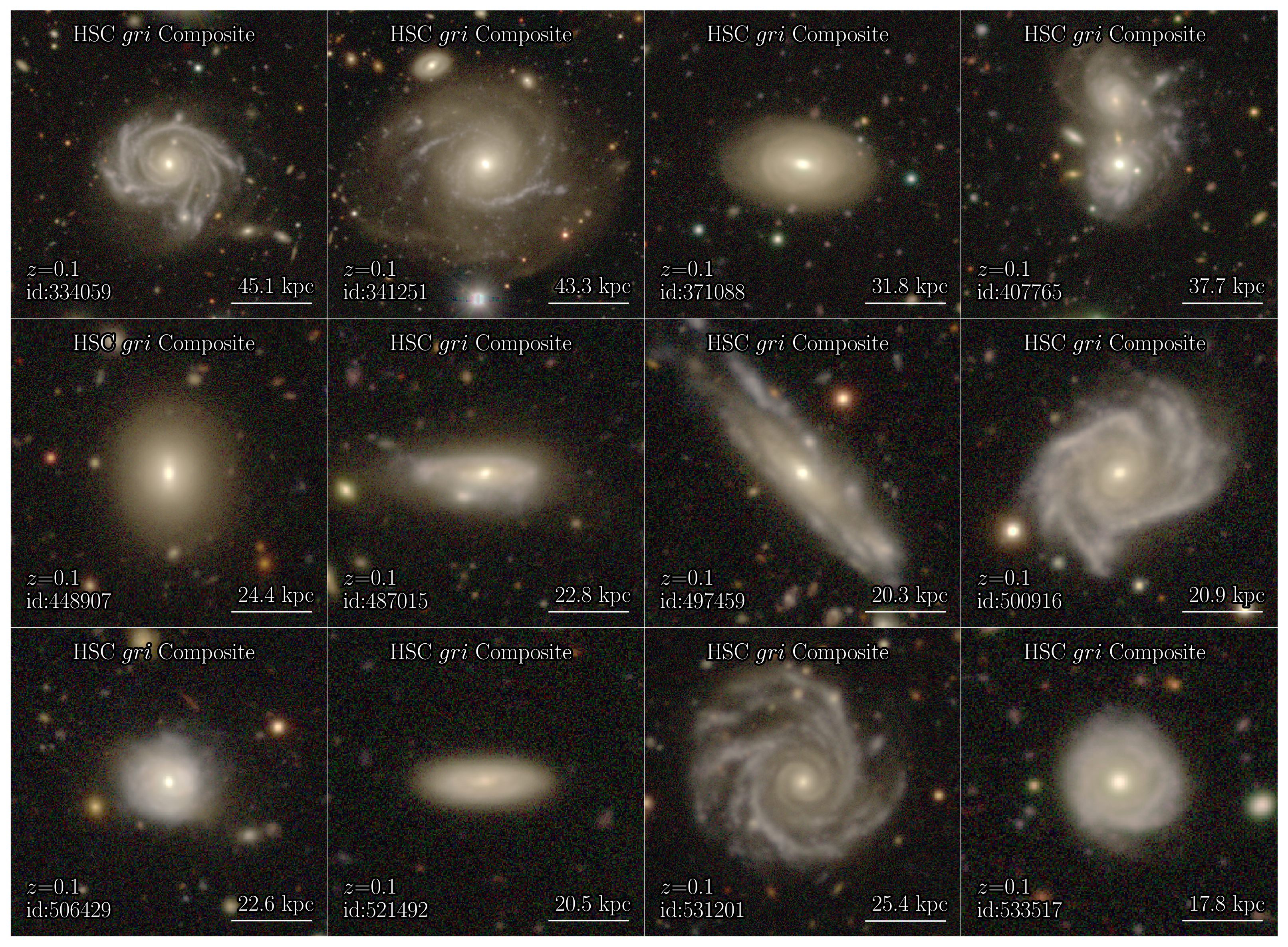
Figure 1: Synthetic forward-modeled $gri$ composite images of galaxies tailored to the HSC-SSP observations. The images are constructed from TNG50 using $\mathtt{SKIRT}$ and stellar population synthesis. They include the realistic survey effects as found in the HSC-SSP. We show 12 randomly selected central galaxies from our data set. The magnitudes, $R_{\rm eff}$, and $CAS$ morphology parameters used in this work are measured from these forward-modeled images.

Next, the survey effects of the HSC-SSP Public Data Release 3 (PDR3; Aihara et al., 2022) are applied to the output images from $\mathtt{SKIRT}$. An adapted version of $\mathtt{RealSim}$ (Bottrell et al., 2019) is used to assign insertion locations, perform flux calibration, spatially rebin to the HSC pixel scale, convolve the images with reconstructed HSC point-spread functions, and insert into realistic HSC-like images. The images have sufficiently large fields-of-view that they include extended structure, satellites, and nearby group/cluster members. Eisert et al (in prep) make a detailed comparison of these TNG50 mocks to real HSC galaxy images and show that their morphologies broadly agree.

After the TNG50 mock images were generated, we carried out photometric and morphological measurements using the GALIGHT surface-brightness decomposition software (Ding et al., 2020). Specifically, we measure magnitudes and effective radii, $R_{\rm eff}$, from parametric Sérsic fits and morphologies quantified by the Concentration, Asymmetry, and Smoothness/Clumpiness (CAS) parameters (Abraham et al., 1994, 1996; Bershady et al., 2000; Conselice, 2003). Since these quantities are measured from the synthetic HSC images, they include realistic measurement uncertainties. In Figure 1, we show forward-modeled $gri$ composite images of 12 randomly selected central galaxies from the data set.

For this paper, we focus on central galaxies at $z=0.1$, classified using the TNG Friends-of-Friends (FoF; Davis et al., 1985) group catalog. For each central galaxy, we compile its true stellar mass ($M_{*}$), true host halo mass ($M_{h}$), and the ‘observed’ $griyz$-band Sérsic magnitudes $\textbf{{X}}_{\rm mag}$, and morphological properties $\textbf{{X}}_{\rm morph}=\{R_{{\rm eff},X},c_{X},A_{X}\}$. The variables $R_{{\rm eff},X},c_{X},A_{X}$ correspond to the characteristic size, concentration, and asymmetry in the $X=g,r,i,z,y$ bands. We also compile the total measured luminosity, $L_{{\rm sat.},X}$, and number, $N_{\rm sat}$, of satellites brighter than $M_{r}<-18$ within each individual group. In total, we use 7,468 photometric measurements from 1,867 simulated central galaxies. We reserve a subset of 125 random central galaxies with $M_{*}>10^{9.5}M_{\odot}$ for testing HaloFlow and use the rest for training.

3 haloFlow

To infer the posterior, $p(\bm{\theta}\,|\,\textbf{{x}})$, of $\bm{\theta}=\{M_{*},M_{h}\}$ given observational measurements, x, we use the HaloFlow SBI framework. SBI enables inference using only a generative model of mock observations. While various SBI approaches have been applied to inference problems in astronomy (e.g. Cameron & Pettitt, 2012; Weyant et al., 2013; Hahn et al., 2017; Alsing et al., 2018; Wong et al., 2020; Zhang et al., 2021), we specifically use an approach based on neural density estimation. In particular, we use “normalizing flow” models (Tabak & Vanden-Eijnden, 2010; Tabak & Turner, 2013), following the SBI approach in SEDFlow (Hahn & Melchior, 2022).

Flows use neural networks to learn an extremely flexible and bijective transformation, $f:x\mapsto z$, that maps a complex target distribution to a simple base distribution, $\pi(\textbf{{z}})$. The target distribution, in our case, is the posterior $p(\bm{\theta}\,|\,\textbf{{x}})$ and $f$ is designed to be invertible and have a tractable Jacobian. This is so that the posterior can be evaluated from $\pi(\textbf{{z}})$ by change of variables. We choose a multivariate Gaussian for $\pi(\textbf{{z}})$, which makes the posterior easy to sample and evaluate. Out of the different flow architectures, we use Masked Autoregressive Flow (MAF; Papamakarios et al., 2017) models as implemented in the $\mathtt{sbi}$ Python package (Greenberg et al., 2019; Tejero-Cantero et al., 2020).

We train a flow, $q_{\bm{\phi}}$, with hyperparameters, $\bm{\phi}$, to best approximate the posterior, $q_{\bm{\phi}}(\bm{\theta}\,|\,\textbf{{x}})\approx p(\bm{\theta}\,|\,\textbf{{x}})$. We split the simulated galaxies into a training and validation set with 90/10 split. Then for galaxies $\{(\bm{\theta}_{i},\textbf{{x}}_{i})\}$ in the training set, we maximize the total log-likelihood $\sum_{i}\log q_{\bm{\phi}}(\bm{\theta}_{i}\,|\,\textbf{{x}}_{i})$. This is equivalent to minimizing the KL divergence between $p(\bm{\theta},\textbf{{x}})=p(\bm{\theta}\,|\,\textbf{{x}})p(\textbf{{x}})$ and $q_{\bm{\phi}}(\bm{\theta}\,|\,\textbf{{x}})p(\textbf{{x}})$. We use the Adam optimizer (Kingma & Ba, 2017) with a learning rate of $5\times 10^{-4}$. To prevent overfitting, we stop training when the log-likelihood evaluated on the validation set fails to increase after 20 consecutive epochs.

To determine our final normalizing flow, we train a large number ($\sim$1000) of flows with architectures determined using the Optuna hyperparameter optimization framework (Akiba et al., 2019). We then select five flows, $q_{\bm{\phi}}^{j}$, with the lowest validation losses and construct our final flow by ensembling them: $q_{\bm{\phi}}(\bm{\theta}\,|\,\textbf{{x}})=\sum_{j=1}^{5}q_{\bm{\phi}}^{j}(\bm{\theta}\,|\,\textbf{{x}})/5$. Ensembling flows with different initializations and architectures improves the accuracy of our normalizing flow (Lakshminarayanan et al., 2016; Alsing et al., 2019).

$q_{\bm{\phi}}$ implicitly includes a prior, $p(\bm{\theta})$, which is set by the $M_{*}$ and $M_{h}$ distribution of our training data set. Without any corrections, this prior reflects the stellar and halo mass functions. Posteriors with this prior would favor low $M_{*}$ and $M_{h}$ values since there are more galaxies with lower $M_{*}$ and $M_{h}$. We correct for this implicit prior and impose uniform priors on $\log M_{*}$ and $\log M_{h}$ using the Handley & Millea (2019) maximum entropy prior method. In practice, for a sample drawn from our posterior, $\bm{\theta}^{\prime}\sim q_{\bm{\phi}}(\bm{\theta}\,|\,\textbf{{x}})$, we impose an importance weight of $1/p(\bm{\theta}^{\prime})$. This ensures that we assume uniform priors on $M_{*}$ and $M_{h}$.

In this work, we make use of different sets of photometric measurements: photometry, photometry and morphology, and etc. For each set of observables, we repeat the entire procedure above and train a separate ensembled flow.

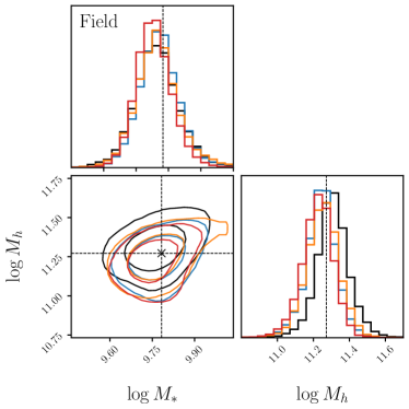
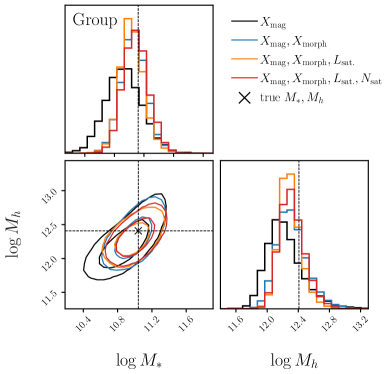
Figure 2: $M_{*}$ and $M_{h}$ posteriors inferred from different sets of photometric measurements: $\{X_{\rm mag}\}$ (black), $\{X_{\rm mag},X_{\rm morph}\}$ (blue), $\{X_{\rm mag},X_{\rm morph},L_{\rm sat}\}$ (orange), and $\{X_{\rm mag},X_{\rm morph},L_{\rm sat},N_{\rm sat}\}$ (red). The contours mark the $68^{\mathrm{th}}$ and $95^{\mathrm{th}}$ percentiles. The left and right set of panels show the posterior for a field and group galaxy, respectively. We also mark the true $M_{*}$ and $M_{h}$ value of the arbitrarily selected simulated galaxy (black $\times$). All of the HaloFlow posteriors are consistent with the true $M_{*}$ and $M_{h}$ values. Furthermore, the posteriors demonstrate that morphology, satellite luminosity, and richness contribute significant additional constraining power for $M_{*}$ and $M_{h}$.

Table 1: HaloFlow median posterior standard error (dex) in stellar mass, $\sigma_{\log M_{*}}$, and halo mass, $\sigma_{\log M_{h}}$, predictions for field and group galaxies relative to ground truth.

HaloFlow Input	Field Galaxies		Group Centrals
	$\sigma_{\log M_{*}}$	$\sigma_{\log M_{h}}$	$\sigma_{\log M_{*}}$	$\sigma_{\log M_{h}}$
$\{X_{\rm mag}\}$	0.096	0.115	0.151	0.182
$\{X_{\rm mag},X_{\rm morph}\}$	0.078	0.105	0.109	0.149
$\{X_{\rm mag},X_{\rm morph},L_{\rm sat}\}$	0.078	0.095	0.118	0.138
$\{X_{\rm mag},X_{\rm morph},L_{\rm sat},N_{\rm sat}\}$	0.073	0.095	0.108	0.132
Standard SHMR Method		0.175		0.208

4 Results

In Figure 2, we present the posteriors of $M_{*}$ and $M_{h}$ for an arbitrarily selected field galaxy (left) and group galaxy (right) inferred using HaloFlow with different sets of observables: $\{X_{\rm mag}\}$ (black), $\{X_{\rm mag},X_{\rm morph}\}$ (blue), $\{X_{\rm mag},X_{\rm morph},L_{\rm sat}\}$ (orange), and $\{X_{\rm mag},X_{\rm morph},L_{\rm sat},N_{\rm sat}\}$ (red). We mark the $68^{\mathrm{th}}$ and $95^{\mathrm{th}}$ percentiles of the posteriors as contours as well as the true $M_{*}$ and $M_{h}$ values of the galaxy (black x). The field galaxy resides in a $M_{h}=10^{11.27}M_{\odot}$ halo and has no satellite galaxies brighter than $M_{r}<-18$; the group galaxy resides in a $M_{h}=10^{12.41}M_{\odot}$ halo and has 7 satellites brighter than $M_{r}<-18$.

All of the HaloFlow posteriors are consistent with each other and in excellent agreement with the true $M_{*}$ and $M_{h}$. For the field galaxy, there is a significant improvement from including $X_{\rm morph}$. However, there is expectedly little improvement from including $L_{\rm sat}$ or $N_{\rm sat}$ since it has no satellite galaxies. The central column of Table 1 summarizes the median standard deviation of HaloFlow posteriors all field central galaxies in the test sample. With the inclusion of $X_{\rm morph},L_{\rm sat},N_{\rm sat}$, we improve the precision of $M_{*}$ and $M_{h}$ constraints for the field galaxy sample by $\sim$0.023 and 0.020 dex — a $\sim$20% improvement.

Meanwhile, for the group central galaxy in Figure 2, including each additional photometric measurement significantly improves the precision of the $M_{*}$ and $M_{h}$ constraints. The median standard deviation of HaloFlow posteriors for all group centrals in the test sample are shown in the right column of Table 1 for each set of observables. Photometric measurements beyond magnitudes, improve the precision of $M_{*}$ and $M_{h}$ constraints by $\sim$0.043 and 0.050 dex — a $\sim$30% improvement.

For both field and group centrals, the HaloFlow posteriors firmly demonstrate that galaxy morphology encodes significant information on both $M_{h}$ and $M_{*}$. This confirms previous works that found connections between morphology and local environment (e.g. Dressler, 1980; Wilman & Erwin, 2012; Pérez-Millán et al., 2023). Our results also show that the photometric measurements of satellite galaxies are informative of $M_{h}$ and $M_{*}$. This is consistent with Tinker et al. (2021), who found that total satellite luminosity is an excellent proxy for $M_{h}$. Beyond confirming previous works, with HaloFlow we precisely quantify the information content of these observables for constraining $M_{*}$ and $M_{h}$. Furthermore, HaloFlow provides a rigorous Bayesian inference framework for actually leveraging these photometric measurements.

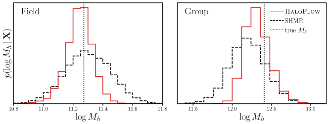
Figure 3: HaloFlow $M_{h}$ posterior using $\{X_{\rm mag},X_{\rm morph},L_{\rm sat},N_{\rm sat}\}$ (red) compared to the $M_{h}$ constraints from the standard approach using the SHMR (black dashed) for the same field (left) and group galaxy (right) as in Figure 2. The $M_{h}$ constraint for the standard method is derived from measuring $M_{*}$ from photometry using SED modeling and then translating it to $M_{h}$ using the SHMR. With HaloFlow, we can exploit the constraining power of $X_{\rm morph}$, $L_{\rm sat}$, and $N_{\rm sat}$ and improve $M_{h}$ constraints by $\sim$0.08 dex ($\sim$40%) over the standard approach.

We further compare the HaloFlow $M_{h}$ posterior (red) to constraints derived from the standard approach (black dashed) for a field (left) and group galaxy (right) in Figure 3. We use the same galaxies as in Figure 2. For the standard approach, we derive the $M_{h}$ constraint by first measuring $M_{*}$ from photometry using SED modeling and then converting $M_{*}$ to $M_{h}$ using the SHMR. We first draw samples from the $M_{*}$ posterior, $M_{*}^{\prime}\sim p(M_{*}\,|\,X_{\rm mag})$, then sample $M_{h}^{\prime}\sim p(M_{h}\,|\,M_{*}^{\prime})$ given by the SHMR. We estimate $p(M_{*}\,|\,X_{\rm mag})$ using HaloFlow and estimate $p(M_{h}\,|\,M_{*}^{\prime})$ from the TNG simulations. This ensures that we do not introduce any biases from discrepant assumptions in the SED modeling (e.g. stellar library, initial mass function, dust modeling) and provides the most “apples to apples” comparisons with HaloFlow. For the HaloFlow posterior, we use the posterior from $\{X_{\rm mag},X_{\rm morph},L_{\rm sat},N_{\rm sat}\}$. With the standard approach, we derive $\sigma_{\log M_{h}}=0.175$ and $0.208$ dex for satellite and group central galaxies, respectively (Table 1). Our HaloFlow $M_{h}$ constraints are significantly, $\gtrsim 0.080$ and $0.076$ dex, tighter than the standard approach. This corresponds to $\sim 40\%$ tighter constraints on $M_{h}$.

In addition to the tighter $M_{h}$ constraints, HaloFlow provides a fully consistent framework for deriving $M_{h}$ directly from observations. In our comparison, as mentioned above, we implement an idealized version of the standard approach where the SED modeling and the SHMR are consistent by construction. However, in practice, the $M_{*}$ derived from SED modeling are not consistent with the $M_{*}$ values used in the SHMR from simulations. The $M_{*}$ from SED modeling is a measurement that depends on the specific assumptions of stellar population synthesis. Depending on modeling choices, the inferred $M_{*}$ can vary by $\sim$ 0.1 dex (Pacifici et al., 2023). Observational effects, such as backgound subtraction (Bernardi et al., 2017), can also significantly impact the $M_{*}$ inferred from SED modeling. Meanwhile, the $M_{*}$ in SHMR is a theoretical quantity, typically derived from summing up the masses of all the star particles in a subhalo. Any discrepancies in the $M_{*}$ measured from SED modeling versus the simulation will bias the inferred $M_{h}$. In HaloFlow, all of these effects are consistently accounted in the forward model.

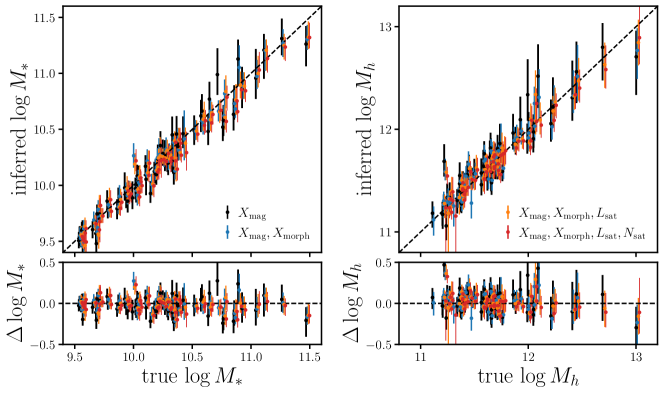
Figure 4: Inferred HaloFlow $M_{*}$ and $M_{h}$ versus the true values for galaxies in our test sample (top panels). The bottom panels show the residuals. We include the posteriors from the different sets of photometric measurements (black, blue, orange, red) and represent their $68^{\mathrm{th}}$ percentiles with the error bars. We include only a subset of the test sample for clarity. Overall, HaloFlow accurately infers the true $M_{*}$ and $M_{h}$. The comparison further confirms that $X_{\rm morph}$, $L_{\rm sat}$, and $N_{\rm sat}$ each significantly tighten the $M_{*}$ and $M_{h}$ posteriors for certain galaxies.

Next, we validate the posteriors from HaloFlow. In Figure 4, we compare the HaloFlow $M_{*}$ and $M_{h}$ inferred from $\{X_{\rm mag}\}$ (black), $\{X_{\rm mag},X_{\rm morph}\}$ (blue), $\{X_{\rm mag},X_{\rm morph},L_{\rm sat}\}$ (orange), and $\{X_{\rm mag},X_{\rm morph},L_{\rm sat},N_{\rm sat}\}$ (red) to the true values (top panels). We show the residuals in the bottom panels. The error bars represent the $68^{\mathrm{th}}$ percentiles of the HaloFlow posteriors. For clarity, we only include 60 of 125 galaxies from the test sample in Figure 4. The comparison illustrates that overall HaloFlow accurately infers the true $M_{*}$ and $M_{h}$. Furthermore, it shows that incorporating $X_{\rm morph}$, $L_{\rm sat}$, and $N_{\rm sat}$ significantly tightens the $M_{*}$ and $M_{h}$ posteriors.

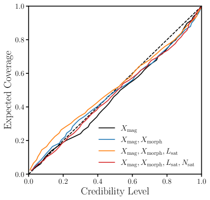
Figure 5: Coverage test validating the accuracy of our HaloFlow posterior estimate using $\{X_{\rm mag}\}$ (black), $\{X_{\rm mag},X_{\rm morph}\}$ (blue), $\{X_{\rm mag},X_{\rm morph},L_{\rm sat}\}$ (orange), and $\{X_{\rm mag},X_{\rm morph},L_{\rm sat},N_{\rm sat}\}$ (red). The test is calculated using the test sample. The black-dashed line represents an optimal estimate of the true posterior. HaloFlow provides a near optimal estimate of the true posterior for all sets of photometric measurements.

As additional validation, we use the Lemos et al. (2023a) “data to random point” (DRP) coverage test. For each test sample, we evaluate distances between samples drawn from HaloFlow posteriors and a random point in parameter space. We compare these distances to the distance between the true $M_{*}$, $M_{h}$ and the random point to derive an estimate of the expected coverage probability. This approach is necessary and sufficient to show that a posterior estimator is optimal. In Figure 5, we present the DRP coverage test of the HaloFlow posteriors for each of the photometric measurements. Significant discrepancies from the true posterior (black-dashed) can reveal whether the posterior estimates are underconfident, overconfident, or biased. In our case, we find no significant discrepancies. Hence, HaloFlow provides near optimal estimates of the true posteriors for all of the adopted combinations of observables.

5 Discussion

HaloFlow leverages state-of-the-art forward modeled galaxy images to exploit additional photometric information that significantly improves constraints on $M_{*}$ and $M_{h}$. Hence, a primary determining factor for the fidelity of HaloFlow is the quality of the forward-model. Below, we discuss the caveats and limitations of our forward-model.

First, our forward model is based on a particular galaxy formation model: that adopted in the TNG cosmological magneto-hydrodynamical simulation. However, previous works have revealed significant discrepancies among the properties of galaxy populations predicted by different state-of-the-art galaxy formation models. Hahn et al. (2019), for instance, found significant discrepancies among the $M_{*}$-star formation rate relations of Illustris, EAGLE, and MUFASA hydrodynamical simulations. Nevertheless, a number of works have demonstrated the success of TNG at reproducing a wide range of observations: e.g. galaxy color bimodality (Nelson et al., 2018), sizes (Genel et al., 2018), optical morphologies (Rodriguez-Gomez et al., 2019; Zanisi et al., 2021), mass-metallicity relation (Torrey et al., 2019), and low redshift quasar luminosity function and black hole mass - stellar bulge mass relation (Weinberger et al., 2018). Furthermore, one of the main relations that HaloFlow exploits from TNG is the SHMR. The SHMR in galaxy formation models is typically calibrated against constraints from observations and, thus, consistent across different models (Wechsler & Tinker, 2018). In TNG, the SHMR is not explicitly calibrated against observational constraints; however, it is indirectly calibrated since the subgrid physics is optimized to match the $z=0$ stellar mass function (Pillepich et al., 2018).

Our forward model also relies on a specific mass-to-light conversion framework. $\mathtt{SKIRT}$ is responsible for generating our synthetic observables from the galaxy physical properties predicted by TNG. The transfer model for the HSC-SSP synthetic images uses the MAPPINGS III SED library to model emission from stellar populations forming in birth-clouds and Bruzual & Charlot (2003) templates for older stellar populations, assuming a Chabrier (2003) initial mass function. These libraries are standard choices in the literature for both SED modeling (e.g. MAGPHYS da Cunha et al. 2015, BEAGLE Chevallard & Charlot 2016, BAGPIPES Carnall et al. 2018) and for radiative transfer modeling (e.g. Torrey et al. 2015; Trayford et al. 2017; Cochrane et al. 2023; Guzmán-Ortega et al. 2023). However, for inferring galaxy properties (i.e. the inverse problem of forward modeling), different SED modeling choices can produce significant discrepancies in galaxy properties, e.g. $M_{*}$ and SFR (Pacifici et al., 2023).

The second component of the mass-to-light conversion framework is the dust model, which handles the scattering and absorption of stellar light by dust. The synthetic images from Bottrell et al. (2023) use a dust model calibrated to gas mass, gas metallicity, and dust mass estimates for galaxies in the local Universe (Rémy-Ruyer et al., 2014; Popping et al., 2022). While empirical, the model is physically intuitive — the gas-to-dust mass ratio should scale with the metal content of the gas at temperatures where dust grains can form. However, there is considerable scatter about the empirical relation for observed galaxies. An in-depth exploration of different SED/dust modeling choices is beyond the scope of this work. But given that significant differences in the inferred physical properties of galaxies arise from the choice of SED and dust modeling this is an area that warrants investigation.

In future works, we will investigate the choices made in our forward-model. For instance, we will train HaloFlow using additional simulations based on other galaxy formation models (e.g. SIMBA, Davé et al. 2019; EAGLE, Crain et al. 2015; Schaye et al. 2015). We will also utilize alternative SPS and dust models. With different forward-models we can improve the robustness of HaloFlow by ensuring that it does not learn relationships among galaxy and halo properties specific to a single galaxy formation model. We will also be able to extensively cross-validate HaloFlow and confirm the robustness of the inferred host halo properties.

These additional simulations will also improve the accuracy of HaloFlow, especially at high $M_{*}$ and $M_{h}$ where there are currently a limited number of simulated galaxies. A larger set of simulated galaxies will also enable more systematic exploration of additional photometric observables that can inform $M_{*}$ and $M_{h}$. Furthermore, with HaloFlow trained on different galaxy formation models, we can precisely quantify the information content of the galaxy-halo connection in each model. The information content will not only serve as an informative statistic of the models but also by comparing across the models we will be able to inform galaxy formation.

In subsequent papers, we will also test and calibrate the HaloFlow $M_{h}$ constraints of observed galaxies and groups in HSC-SSP against constraints from galaxy-galaxy weak lensing measurements (e.g. Rana et al., 2022). We will also compare them to dynamical mass estimates of groups identified in GAMA (Driver et al., 2022). Once validated, we will apply HaloFlow to intervening halos observed by the FLIMFLAM spectroscopic survey (Lee et al., 2022) targeting FRB foreground fields to enhance their constraints on the CGM baryonic fraction.

Lastly, we limited the $L_{\rm sat}$ and $N_{\rm sat}$ measurements to satellite galaxies with $M_{r}<-18$ in this work. Including fainter galaxies in $L_{\rm sat}$ and $N_{\rm sat}$ would further improve the precision of HaloFlow. Future observations from DESI and Rubin, which will probe significantly fainter galaxies, will be able to take advantage of the additional gains from HaloFlow.

6 Summary

We present HaloFlow, a framework for inferring host halo masses from the photometry and morphology of galaxies using simulation-based inference (SBI) with normalizing flows. HaloFlow is specifically tailored to galaxies in the Hyper Suprime-Cam Subaru Strategy Program (HSC-SSP) and, thus, leverages state-of-the-art synthetic galaxy images that model the realistic effects of the HSC-SSP observations (Bottrell et al., 2023). These images are constructed from the TNG hydrodynamic simulations using the $\mathtt{SKIRT}$ dust radiative transfer and an adapted version of $\mathtt{RealSim}$.

We train HaloFlow using 7,468 photometric measurements of 1,867 central galaxies made on the synthetic HSC images using GALIGHT. The measurements include $grizy$-band magnitudes ($X_{\rm mag}$), $CAS$ morphological parameters ($X_{\rm morph}$), total measured satellite luminosities ($L_{\rm sat}$), and number of satellites ($N_{\rm sat}$). HaloFlow uses normalizing flows to perform neural density estimation of the posterior, $p(\bm{\theta}\,|\,\textbf{{x}})$, of $\bm{\theta}=\{M_{*},M_{h}\}$ given the photometric measurements. We follow the SBI approach of Hahn & Melchior (2022) with two additional steps. First, our final flow is derived from ensembling the five flows with the lowest validation losses. Second, we correct for the implicit prior on $M_{*}$ and $M_{h}$ set by the stellar and halo mass functions using the Handley & Millea (2019) maximum entropy prior method. We train separate flows, $q_{\phi}(\bm{\theta}\,|\,\textbf{{x}})\approx p(\bm{\theta}\,|\,\textbf{{x}})$, for different sets of photometric measurements, $\textbf{{x}}=\{X_{\rm mag}\}$, $\{X_{\rm mag},X_{\rm morph}\}$, $\{X_{\rm mag},X_{\rm morph},L_{\rm sat}\}$, $\{X_{\rm mag},X_{\rm morph},L_{\rm sat},N_{\rm sat}\}$.

When we apply HaloFlow to a subset of 125 random central galaxies with $M_{*}>10^{9.5}M_{\odot}$ excluded from the training we find:

• HaloFlow successfully infers posteriors that are consistent with the true $M_{*}$ and $M_{h}$ for every set of photometric measurements. We further validate the accuracy of the posteriors using the Lemos et al. (2023b) DRP cover test and confirm that HaloFlow provides near optimal estimates of the true posteriors.

• Comparison of the HaloFlow posteriors firmly demonstrate that galaxy morphology encodes significant information on both $M_{*}$ and $M_{h}$. This confirms and quantifies the known connection between morphology and local environment. The HaloFlow posteriors also show that satellite measurements can further improve $M_{h}$ constraints. With these additional observables, we can improve $M_{h}$ constraints by $\sim$20 and 30% for field and group galaxies, respectively.

• With all of our photometric measurements, we can constrain $M_{*}$ and $M_{h}$ with precision levels of $\sigma_{\log M_{*}}\sim 0.073$ and $\sigma_{\log M_{h}}\sim 0.095$ dex for field galaxies and $\sigma_{\log M_{*}}\sim 0.108$ and $\sigma_{\log M_{h}}\sim 0.132$ dex for group galaxies. Our HaloFlow $M_{h}$ constraints are $\sim$40% tighter than standard $M_{h}$ methods based on the SHMR.

HaloFlow uses SBI to leverage state-of-the-art synthetic galaxy images. Its fidelity is, therefore, determined by the quality of the forward model used to simulate the images. Our forward model relies on the TNG galaxy formation model, which has been show to successfully reproduce a wide range of observations. It also relies on $\mathtt{SKIRT}$, which uses standard modeling choices in the literature. Nevertheless, in future work we will go beyond these choices and use additional galaxy formation models and alternative SPS and dust models to improve the robustness of HaloFlow. We will also further validate HaloFlow using alternative methods for inferring $M_{h}$ based on galaxy-galaxy weak lensing. Afterwards, we will apply HaloFlow to HSC-SSP and infer $M_{h}$ for a variety of applications: e.g. constrainig $M_{h}$ of halos in the foreground of FRBs to place stringent constraints on the CGM baryonic fraction.

References

- Abraham et al. (1994) Abraham, R. G., Valdes, F., Yee, H. K. C., & van den Bergh, S. 1994, The Astrophysical Journal, 432, 75, doi: 10.1086/174550
- Abraham et al. (1996) Abraham, R. G., van den Bergh, S., Glazebrook, K., et al. 1996, The Astrophysical Journal Supplement Series, 107, 1, doi: 10.1086/192352
- Aihara et al. (2022) Aihara, H., AlSayyad, Y., Ando, M., et al. 2022, Publications of the Astronomical Society of Japan, 74, 247, doi: 10.1093/pasj/psab122
- Akiba et al. (2019) Akiba, T., Sano, S., Yanase, T., Ohta, T., & Koyama, M. 2019, in Proceedings of the 25th ACM SIGKDD international conference on knowledge discovery & data mining, 2623–2631
- Albrecht et al. (2006) Albrecht, A., Bernstein, G., Cahn, R., et al. 2006, arXiv e-prints, astro, doi: 10.48550/arXiv.astro-ph/0609591
- Allen et al. (2011) Allen, S. W., Evrard, A. E., & Mantz, A. B. 2011, ARA&A, 49, 409, doi: 10.1146/annurev-astro-081710-102514
- Alsing et al. (2019) Alsing, J., Charnock, T., Feeney, S., & Wandelt, B. 2019, Monthly Notices of the Royal Astronomical Society, 488, 4440, doi: 10.1093/mnras/stz1960
- Alsing et al. (2018) Alsing, J., Wandelt, B., & Feeney, S. 2018, arXiv:1801.01497 [astro-ph]. https://arxiv.org/abs/1801.01497
- Baes et al. (2011) Baes, M., Verstappen, J., De Looze, I., et al. 2011, ApJS, 196, 22, doi: 10.1088/0067-0049/196/2/22
- Baldry et al. (2006) Baldry, I. K., Balogh, M. L., Bower, R. G., et al. 2006, MNRAS, 373, 469, doi: 10.1111/j.1365-2966.2006.11081.x
- Behroozi et al. (2019) Behroozi, P., Wechsler, R. H., Hearin, A. P., & Conroy, C. 2019, MNRAS, 488, 3143, doi: 10.1093/mnras/stz1182
- Bernardi et al. (2017) Bernardi, M., Meert, A., Sheth, R. K., et al. 2017, MNRAS, 467, 2217, doi: 10.1093/mnras/stx176
- Bershady et al. (2000) Bershady, M. A., Jangren, A., & Conselice, C. J. 2000, The Astronomical Journal, 119, 2645, doi: 10.1086/301386
- Blanton et al. (2005) Blanton, M. R., Eisenstein, D., Hogg, D. W., Schlegel, D. J., & Brinkmann, J. 2005, ApJ, 629, 143, doi: 10.1086/422897
- Blanton & Moustakas (2009) Blanton, M. R., & Moustakas, J. 2009, ARA&A, 47, 159, doi: 10.1146/annurev-astro-082708-101734
- Bottrell et al. (2019) Bottrell, C., Hani, M. H., Teimoorinia, H., et al. 2019, MNRAS, 490, 5390, doi: 10.1093/mnras/stz2934
- Bottrell et al. (2023) Bottrell, C., Yesuf, H. M., Popping, G., et al. 2023, arXiv e-prints, arXiv:2308.14793, doi: 10.48550/arXiv.2308.14793
- Bregman (2007) Bregman, J. N. 2007, ARA&A, 45, 221, doi: 10.1146/annurev.astro.45.051806.110619
- Bruzual & Charlot (2003) Bruzual, G., & Charlot, S. 2003, Monthly Notices of the Royal Astronomical Society, 344, 1000, doi: 10.1046/j.1365-8711.2003.06897.x
- Cacciato et al. (2009) Cacciato, M., van den Bosch, F. C., More, S., et al. 2009, MNRAS, 394, 929, doi: 10.1111/j.1365-2966.2008.14362.x
- Cacciato et al. (2013) Cacciato, M., van den Bosch, F. C., More, S., Mo, H., & Yang, X. 2013, MNRAS, 430, 767, doi: 10.1093/mnras/sts525
- Calderon & Berlind (2019) Calderon, V. F., & Berlind, A. A. 2019, MNRAS, 490, 2367, doi: 10.1093/mnras/stz2775
- Cameron & Pettitt (2012) Cameron, E., & Pettitt, A. N. 2012, Monthly Notices of the Royal Astronomical Society, 425, 44, doi: 10.1111/j.1365-2966.2012.21371.x
- Camps & Baes (2015) Camps, P., & Baes, M. 2015, Astronomy and Computing, 9, 20, doi: 10.1016/j.ascom.2014.10.004
- Camps & Baes (2020) —. 2020, Astronomy and Computing, 31, 100381, doi: 10.1016/j.ascom.2020.100381
- Carnall et al. (2018) Carnall, A. C., McLure, R. J., Dunlop, J. S., & Davé, R. 2018, MNRAS, 480, 4379, doi: 10.1093/mnras/sty2169
- Cen & Ostriker (2006) Cen, R., & Ostriker, J. P. 2006, ApJ, 650, 560, doi: 10.1086/506505
- Chabrier (2003) Chabrier, G. 2003, Publications of the Astronomical Society of the Pacific, 115, 763, doi: 10.1086/376392
- Chevallard & Charlot (2016) Chevallard, J., & Charlot, S. 2016, MNRAS, 462, 1415, doi: 10.1093/mnras/stw1756
- Cochrane et al. (2023) Cochrane, R. K., Hayward, C. C., Anglés-Alcázar, D., & Somerville, R. S. 2023, MNRAS, 518, 5522, doi: 10.1093/mnras/stac3451
- Conselice (2003) Conselice, C. J. 2003, The Astrophysical Journal Supplement Series, 147, 1, doi: 10.1086/375001
- Cordes & Chatterjee (2019) Cordes, J. M., & Chatterjee, S. 2019, ARA&A, 57, 417, doi: 10.1146/annurev-astro-091918-104501
- Crain et al. (2015) Crain, R. A., Schaye, J., Bower, R. G., et al. 2015, MNRAS, 450, 1937, doi: 10.1093/mnras/stv725
- da Cunha et al. (2015) da Cunha, E., Walter, F., Smail, I. R., et al. 2015, ApJ, 806, 110, doi: 10.1088/0004-637X/806/1/110
- Davé et al. (2019) Davé, R., Anglés-Alcázar, D., Narayanan, D., et al. 2019, MNRAS, 486, 2827, doi: 10.1093/mnras/stz937
- Davis et al. (1985) Davis, M., Efstathiou, G., Frenk, C. S., & White, S. D. M. 1985, The Astrophysical Journal, 292, 371, doi: 10.1086/163168
- Davis & Geller (1976) Davis, M., & Geller, M. J. 1976, ApJ, 208, 13, doi: 10.1086/154575
- Ding et al. (2020) Ding, X., Silverman, J., Treu, T., et al. 2020, ApJ, 888, 37, doi: 10.3847/1538-4357/ab5b90
- Dodelson et al. (2016) Dodelson, S., Heitmann, K., Hirata, C., et al. 2016, arXiv e-prints, arXiv:1604.07626, doi: 10.48550/arXiv.1604.07626
- Dressler (1980) Dressler, A. 1980, ApJ, 236, 351, doi: 10.1086/157753
- Driver et al. (2022) Driver, S. P., Robotham, A. S. G., Obreschkow, D., et al. 2022, MNRAS, 515, 2138, doi: 10.1093/mnras/stac581
- Fukugita & Peebles (2004) Fukugita, M., & Peebles, P. J. E. 2004, ApJ, 616, 643, doi: 10.1086/425155
- Genel et al. (2018) Genel, S., Nelson, D., Pillepich, A., et al. 2018, MNRAS, 474, 3976, doi: 10.1093/mnras/stx3078
- Greenberg et al. (2019) Greenberg, D. S., Nonnenmacher, M., & Macke, J. H. 2019, Automatic Posterior Transformation for Likelihood-Free Inference
- Groves et al. (2008) Groves, B., Dopita, M. A., Sutherland, R. S., et al. 2008, ApJS, 176, 438, doi: 10.1086/528711
- Guzmán-Ortega et al. (2023) Guzmán-Ortega, A., Rodriguez-Gomez, V., Snyder, G. F., Chamberlain, K., & Hernquist, L. 2023, MNRAS, 519, 4920, doi: 10.1093/mnras/stac3334
- Hahn & Melchior (2022) Hahn, C., & Melchior, P. 2022, Accelerated Bayesian SED Modeling Using Amortized Neural Posterior Estimation
- Hahn et al. (2017) Hahn, C., Vakili, M., Walsh, K., et al. 2017, Monthly Notices of the Royal Astronomical Society, 469, 2791, doi: 10.1093/mnras/stx894
- Hahn et al. (2015) Hahn, C., Blanton, M. R., Moustakas, J., et al. 2015, ApJ, 806, 162, doi: 10.1088/0004-637X/806/2/162
- Hahn et al. (2019) Hahn, C., Starkenburg, T. K., Choi, E., et al. 2019, ApJ, 872, 160, doi: 10.3847/1538-4357/aafedd
- Handley & Millea (2019) Handley, W., & Millea, M. 2019, Entropy, 21, 272, doi: 10.3390/e21030272
- Hearin et al. (2013) Hearin, A. P., Zentner, A. R., Berlind, A. A., & Newman, J. A. 2013, MNRAS, 433, 659, doi: 10.1093/mnras/stt755
- Hogg et al. (2004) Hogg, D. W., Blanton, M. R., Brinchmann, J., et al. 2004, ApJ, 601, L29, doi: 10.1086/381749
- Huang et al. (2020) Huang, S., Leauthaud, A., Hearin, A., et al. 2020, MNRAS, 492, 3685, doi: 10.1093/mnras/stz3314
- Ivezić et al. (2019) Ivezić, Ž., Kahn, S. M., Tyson, J. A., et al. 2019, ApJ, 873, 111, doi: 10.3847/1538-4357/ab042c
- Kauffmann et al. (2004) Kauffmann, G., White, S. D. M., Heckman, T. M., et al. 2004, MNRAS, 353, 713, doi: 10.1111/j.1365-2966.2004.08117.x
- Kawanomoto et al. (2018) Kawanomoto, S., Uraguchi, F., Komiyama, Y., et al. 2018, Publications of the Astronomical Society of Japan, 70, 66, doi: 10.1093/pasj/psy056
- Khrykin et al. (2023) Khrykin, I. S., Sorini, D., Lee, K.-G., & Davé, R. 2023, The Cosmic Baryon Partition between the IGM and CGM in the SIMBA Simulations. https://arxiv.org/abs/2310.01496
- Kingma & Ba (2017) Kingma, D. P., & Ba, J. 2017, arXiv:1412.6980 [cs]. https://arxiv.org/abs/1412.6980
- Kravtsov et al. (2004) Kravtsov, A. V., Berlind, A. A., Wechsler, R. H., et al. 2004, ApJ, 609, 35, doi: 10.1086/420959
- Kravtsov & Borgani (2012) Kravtsov, A. V., & Borgani, S. 2012, ARA&A, 50, 353, doi: 10.1146/annurev-astro-081811-125502
- Lakshminarayanan et al. (2016) Lakshminarayanan, B., Pritzel, A., & Blundell, C. 2016, arXiv e-prints, arXiv:1612.01474, doi: 10.48550/arXiv.1612.01474
- Lange et al. (2019) Lange, J. U., van den Bosch, F. C., Zentner, A. R., Wang, K., & Villarreal, A. S. 2019, MNRAS, 482, 4824, doi: 10.1093/mnras/sty2950
- Lee et al. (2022) Lee, K.-G., Ata, M., Khrykin, I. S., et al. 2022, ApJ, 928, 9, doi: 10.3847/1538-4357/ac4f62
- Lee et al. (2023) Lee, K.-G., Khrykin, I. S., Simha, S., et al. 2023, ApJ, 954, L7, doi: 10.3847/2041-8213/acefb5
- Lemos et al. (2023a) Lemos, P., Coogan, A., Hezaveh, Y., & Perreault-Levasseur, L. 2023a, arXiv preprint arXiv:2302.03026
- Lemos et al. (2023b) Lemos, P., Cranmer, M., Abidi, M., et al. 2023b, Machine Learning: Science and Technology, 4, 01LT01
- Ludlow et al. (2021) Ludlow, A. D., Fall, S. M., Schaye, J., & Obreschkow, D. 2021, MNRAS, 508, 5114, doi: 10.1093/mnras/stab2770
- Ludlow et al. (2023) Ludlow, A. D., Fall, S. M., Wilkinson, M. J., Schaye, J., & Obreschkow, D. 2023, MNRAS, 525, 5614, doi: 10.1093/mnras/stad2615
- Macquart et al. (2020) Macquart, J. P., Prochaska, J. X., McQuinn, M., et al. 2020, Nature, 581, 391, doi: 10.1038/s41586-020-2300-2
- Mandelbaum et al. (2006) Mandelbaum, R., Seljak, U., Cool, R. J., et al. 2006, MNRAS, 372, 758, doi: 10.1111/j.1365-2966.2006.10906.x
- Mandelbaum et al. (2016) Mandelbaum, R., Wang, W., Zu, Y., et al. 2016, MNRAS, 457, 3200, doi: 10.1093/mnras/stw188
- Mantz et al. (2015) Mantz, A. B., von der Linden, A., Allen, S. W., et al. 2015, MNRAS, 446, 2205, doi: 10.1093/mnras/stu2096
- Marinacci et al. (2018) Marinacci, F., Vogelsberger, M., Pakmor, R., et al. 2018, MNRAS, 480, 5113, doi: 10.1093/mnras/sty2206
- McQuinn (2014) McQuinn, M. 2014, ApJ, 780, L33, doi: 10.1088/2041-8205/780/2/L33
- More et al. (2009) More, S., van den Bosch, F. C., & Cacciato, M. 2009, MNRAS, 392, 917, doi: 10.1111/j.1365-2966.2008.14114.x
- More et al. (2011) More, S., van den Bosch, F. C., Cacciato, M., et al. 2011, MNRAS, 410, 210, doi: 10.1111/j.1365-2966.2010.17436.x
- Moster et al. (2018) Moster, B. P., Naab, T., & White, S. D. M. 2018, MNRAS, 477, 1822, doi: 10.1093/mnras/sty655
- Naiman et al. (2018) Naiman, J. P., Pillepich, A., Springel, V., et al. 2018, MNRAS, 477, 1206, doi: 10.1093/mnras/sty618
- Nelson et al. (2018) Nelson, D., Pillepich, A., Springel, V., et al. 2018, Monthly Notices of the Royal Astronomical Society, 475, 624, doi: 10.1093/mnras/stx3040
- Nelson et al. (2019) Nelson, D., Springel, V., Pillepich, A., et al. 2019, Computational Astrophysics and Cosmology, 6, 2, doi: 10.1186/s40668-019-0028-x
- Norberg et al. (2008) Norberg, P., Frenk, C. S., & Cole, S. 2008, MNRAS, 383, 646, doi: 10.1111/j.1365-2966.2007.12583.x
- Ntampaka et al. (2015) Ntampaka, M., Trac, H., Sutherland, D. J., et al. 2015, ApJ, 803, 50, doi: 10.1088/0004-637X/803/2/50
- Ntampaka et al. (2016) —. 2016, ApJ, 831, 135, doi: 10.3847/0004-637X/831/2/135
- Oemler (1974) Oemler, Augustus, J. 1974, ApJ, 194, 1, doi: 10.1086/153216
- Old et al. (2014) Old, L., Skibba, R. A., Pearce, F. R., et al. 2014, MNRAS, 441, 1513, doi: 10.1093/mnras/stu545
- Old et al. (2015) Old, L., Wojtak, R., Mamon, G. A., et al. 2015, MNRAS, 449, 1897, doi: 10.1093/mnras/stv421
- Old et al. (2018) Old, L., Wojtak, R., Pearce, F. R., et al. 2018, MNRAS, 475, 853, doi: 10.1093/mnras/stx3241
- Pacifici et al. (2023) Pacifici, C., Iyer, K. G., Mobasher, B., et al. 2023, ApJ, 944, 141, doi: 10.3847/1538-4357/acacff
- Papamakarios et al. (2017) Papamakarios, G., Pavlakou, T., & Murray, I. 2017, arXiv e-prints, 1705, arXiv:1705.07057
- Pérez-Millán et al. (2023) Pérez-Millán, D., Fritz, J., González-Lópezlira, R. A., et al. 2023, MNRAS, 521, 1292, doi: 10.1093/mnras/stad542
- Pillepich et al. (2018) Pillepich, A., Springel, V., Nelson, D., et al. 2018, Monthly Notices of the Royal Astronomical Society, 473, 4077, doi: 10.1093/mnras/stx2656
- Pillepich et al. (2018) Pillepich, A., Nelson, D., Hernquist, L., et al. 2018, MNRAS, 475, 648, doi: 10.1093/mnras/stx3112
- Popping et al. (2022) Popping, G., Pillepich, A., Calistro Rivera, G., et al. 2022, MNRAS, 510, 3321, doi: 10.1093/mnras/stab3312
- Prochaska & Zheng (2019) Prochaska, J. X., & Zheng, Y. 2019, MNRAS, 485, 648, doi: 10.1093/mnras/stz261
- Rana et al. (2022) Rana, D., More, S., Miyatake, H., et al. 2022, MNRAS, 510, 5408, doi: 10.1093/mnras/stac007
- Rémy-Ruyer et al. (2014) Rémy-Ruyer, A., Madden, S. C., Galliano, F., et al. 2014, A&A, 563, A31, doi: 10.1051/0004-6361/201322803
- Rodriguez-Gomez et al. (2019) Rodriguez-Gomez, V., Snyder, G. F., Lotz, J. M., et al. 2019, MNRAS, 483, 4140, doi: 10.1093/mnras/sty3345
- Schaye et al. (2015) Schaye, J., Crain, R. A., Bower, R. G., et al. 2015, MNRAS, 446, 521, doi: 10.1093/mnras/stu2058
- Springel (2010) Springel, V. 2010, 401, 791, doi: 10.1111/j.1365-2966.2009.15715.x
- Springel et al. (2018) Springel, V., Pakmor, R., Pillepich, A., et al. 2018, Monthly Notices of the Royal Astronomical Society, 475, 676, doi: 10.1093/mnras/stx3304
- Tabak & Turner (2013) Tabak, E. G., & Turner, C. V. 2013, Communications on Pure and Applied Mathematics, 66, 145, doi: 10.1002/cpa.21423
- Tabak & Vanden-Eijnden (2010) Tabak, E. G., & Vanden-Eijnden, E. 2010, Communications in Mathematical Sciences, 8, 217, doi: 10.4310/CMS.2010.v8.n1.a11
- Tasitsiomi et al. (2004) Tasitsiomi, A., Kravtsov, A. V., Wechsler, R. H., & Primack, J. R. 2004, ApJ, 614, 533, doi: 10.1086/423784
- Tejero-Cantero et al. (2020) Tejero-Cantero, A., Boelts, J., Deistler, M., et al. 2020, Journal of Open Source Software, 5, 2505, doi: 10.21105/joss.02505
- Tinker et al. (2011) Tinker, J., Wetzel, A., & Conroy, C. 2011, arXiv e-prints, arXiv:1107.5046, doi: 10.48550/arXiv.1107.5046
- Tinker (2022) Tinker, J. L. 2022, AJ, 163, 126, doi: 10.3847/1538-3881/ac37bb
- Tinker et al. (2021) Tinker, J. L., Cao, J., Alpaslan, M., et al. 2021, MNRAS, 505, 5370, doi: 10.1093/mnras/stab1576
- Torrey et al. (2015) Torrey, P., Snyder, G. F., Vogelsberger, M., et al. 2015, MNRAS, 447, 2753, doi: 10.1093/mnras/stu2592
- Torrey et al. (2019) Torrey, P., Vogelsberger, M., Marinacci, F., et al. 2019, MNRAS, 484, 5587, doi: 10.1093/mnras/stz243
- Trayford et al. (2017) Trayford, J. W., Camps, P., Theuns, T., et al. 2017, MNRAS, 470, 771, doi: 10.1093/mnras/stx1051
- Vale & Ostriker (2004) Vale, A., & Ostriker, J. P. 2004, MNRAS, 353, 189, doi: 10.1111/j.1365-2966.2004.08059.x
- Villanueva-Domingo et al. (2022) Villanueva-Domingo, P., Villaescusa-Navarro, F., Anglés-Alcázar, D., et al. 2022, ApJ, 935, 30, doi: 10.3847/1538-4357/ac7aa3
- Voit (2005) Voit, G. M. 2005, Reviews of Modern Physics, 77, 207, doi: 10.1103/RevModPhys.77.207
- Wechsler & Tinker (2018) Wechsler, R. H., & Tinker, J. L. 2018, ARA&A, 56, 435, doi: 10.1146/annurev-astro-081817-051756
- Weinberg et al. (2013) Weinberg, D. H., Mortonson, M. J., Eisenstein, D. J., et al. 2013, Phys. Rep., 530, 87, doi: 10.1016/j.physrep.2013.05.001
- Weinberger et al. (2018) Weinberger, R., Springel, V., Pakmor, R., et al. 2018, Monthly Notices of the Royal Astronomical Society, 479, 4056, doi: 10.1093/mnras/sty1733
- Weingartner & Draine (2001) Weingartner, J. C., & Draine, B. T. 2001, ApJ, 548, 296, doi: 10.1086/318651
- Weyant et al. (2013) Weyant, A., Schafer, C., & Wood-Vasey, W. M. 2013, The Astrophysical Journal, 764, 116, doi: 10.1088/0004-637X/764/2/116
- Wilman & Erwin (2012) Wilman, D. J., & Erwin, P. 2012, ApJ, 746, 160, doi: 10.1088/0004-637X/746/2/160
- Wojtak et al. (2018) Wojtak, R., Old, L., Mamon, G. A., et al. 2018, MNRAS, 481, 324, doi: 10.1093/mnras/sty2257
- Wong et al. (2020) Wong, K. W. K., Contardo, G., & Ho, S. 2020, Physical Review D, 101, 123005, doi: 10.1103/PhysRevD.101.123005
- Yang et al. (2009) Yang, X., Mo, H. J., & van den Bosch, F. C. 2009, ApJ, 695, 900, doi: 10.1088/0004-637X/695/2/900
- Zanisi et al. (2021) Zanisi, L., Huertas-Company, M., Lanusse, F., et al. 2021, MNRAS, 501, 4359, doi: 10.1093/mnras/staa3864
- Zhang et al. (2021) Zhang, K., Bloom, J. S., Gaudi, B. S., et al. 2021, doi: 10.3847/1538-3881/abf42e