Signatures of Domain-Wall Confinement in Raman Spectroscopy of Ising Spin Chains

Abstract

Mesonic bound states of domain walls can be stabilized in quasi one-dimensional magnetic compounds. Here, we theoretically study the Raman light scattering response of a twisted Kitaev chain with tilted magnetic fields as a minimal model for confinement in CoNb2O6. By both numerical matrix product states and few-domain wall variational states, we show that confinement-induced bound states directly manifest themselves as sharp peaks in the Raman response. Near quantum criticality the Raman spectrum exhibit the famous E₈ symmetry. Remarkably, by tuning the polarization of the incident light field, we demonstrate that the Raman response offers new insights into the intrinsic structure of the bound state wavefunction.

Introduction. – Confinement of excitations is traditionally considered as a phenomenon of high-energy physics. However, over the recent years, related effects have been discussed in condensed matter settings as well. A paradigmatic example is the formation of mesonic bound states in spin chains that exhibit a linear confinement potential between domain walls [1, 2, 3, 4, 5, 6]. A prominent candidate material to realize this effect is the quasi one-dimensional (1D) magnetic compound CoNb2O6, often discussed as a paradigmatic example for a quantum Ising magnet in a longitudinal and transverse field [7, 8, 9, 10, 11, 12, 13, 14, 2, 15, 16, 17]. First experimental studies of domain-wall confinement in CoNb2O6 were achieved with neutron scattering [2] and terahertz spectroscopy [18]. Further experimental and theoretical studies refined the model Hamiltonian to capture additional structure beyond the conventional Ising chain [19, 20, 21, 22, 23, 2, 24, 25, 26, 27]. Applying external fields, even allowed studies of confinement in the vicinity of the quantum critical point, resulting in an emergent $E_{8}$-symmetry in the spectral response [2, 25, 6].

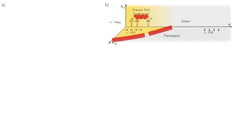
Figure 1: Raman response of confined domain walls in a twisted Kitaev magnet. (a) Schematic structure of a set of quasi one-dimensional chains forming CoNb2O6, that are characterized by a zigzag angle $\vartheta$. Raman light scattering processes of incoming photons with polarization $\hat{e}_{i}$ and outgoing photons with polarization $\hat{e}_{f}$ couple differently to even and odd bonds of the chain. (b) For a given zigzag angle $\vartheta$ and transverse field $h_{y}$, the ground state is either a ferromagnet aligned with one of the planar direction of the chain or a paramagnet. Applying a magnetic field along the hard axis of the ferromagnet confines the low-energy domain wall (DW) excitations (yellow area for $h_{x}$ field). Along the Ising quantum critical line (red dashed) the spectrum is expected to possess an emergent anomalous $E_{8}$-symmetry. (c) Raman response for different twist angles $\vartheta\in\{\frac{\pi}{16},\frac{\pi}{8},\frac{\pi}{4}\}$ and longitudinal fields $h_{x}=0,0.05$, and $0.2$ change from a two DW continuum to discrete peaks, resulting from the bound states of confined DWs. Bottom row: Deep in the ferromagnetic phase the numerical results from iMPS simulations are well captured by a few-soliton ansatz considering only 2 (green markers) or 4 (red markers) DWs.

Here, we propose Raman spectroscopy as a complementary tool for studying confinement effects in solids. We consider a twisted Kitaev spin chain as a minimal model for CoNb2O6 and demonstrate that domain wall confinement manifests itself as sharp spectral peaks in the Raman response. We compute the Raman spectra numerically with Matrix Product States (MPS) as well as with few-soliton variational states. The latter correctly capture the bound state physics in the most part of the phase diagram, except near quantum criticality, where the spectrum exhibits the famous E₈ symmetry and the bound state structure is involved. As a key result, we show that excitations can be selectively addressed by tuning the polarization of the photons, which provides additional information about the intrinsic structure of the bound states.

Model. – For our analysis we will consider a minimal model allowing us to qualitatively reproduce the key signatures observed for the magnetic compound CoNb2O6 [23]. The model captures the essential low energy physics by taking into account a zigzag geometry for the quasi one-dimensional building blocks of CoNb2O6, see Fig. 1 (a). Thereby, the spins are assumed to interact solely within a zigzag chain. The resulting model is typically referred to as the twisted Kitaev (TK) Hamiltonian

$$\mathcal{H}_{\mathrm{TK}}=\sum_{j} -\Big{[}\cos^{2}\Big{(}\frac{\vartheta}{2}\Big{)}\sigma_{j}^{x}\sigma_{j+1}^{x}+\sin^{2}\Big{(}\frac{\vartheta}{2}\Big{)}\sigma_{j}^{z}\sigma_{j+1}^{z}$$

$$+\frac{1}{2}\sin(\vartheta)(-1)^{j}\big{(}\sigma_{j}^{z}\sigma_{j+1}^{x}+\sigma_{j}^{x}\sigma_{j+1}^{z}\big{)}\Big{]}.$$ (1)

The zigzag angle $\vartheta$ interpolates between Ising ferromagnets orientated in $\hat{x}$- and $\hat{z}$-direction for $\vartheta=0$ and $\vartheta=\pi$, respectively, and a rotated version of the Kitaev chain for $\vartheta=\frac{\pi}{2}$. The weak inter-chain coupling present in actual materials is typically taken into account on a mean-field level, giving rise to an external magnetic field contribution

$$\mathcal{H}=\mathcal{H}_{\mathrm{TK}}-\frac{1}{2}\sum_{j}\Big{[}h_{x}\sigma_{j}^{x}+h_{y}\sigma_{j}^{y}+h_{z}\sigma_{j}^{z}\Big{]}.$$ (2)

The effective magnetic fields $h_{x}$, $h_{y}$, and $h_{z}$ are tuneable experimentally by external fields. For a $\hat{y}$-polarized magnetic field, that is transverse to the ferromagnetic orders of Eq. (1), the model is analytically solvable by a a Jordan-Wigner transformation that maps the model to free fermions [22, 28]. The ground state phase diagram of that limit is sketched in Fig. 1 (b) in the $(\vartheta,h_{y})$-plane. An infinitesimal magnetic field along either of the remaining two directions $\hat{x},\hat{z}$ breaks the integrability of the model. When perturbing the ferromagnetic phases these fields can manifest themselves in two fundamentally different ways: (i) Applying an additional field transverse to the ferromagnet, decorates the domain walls and modifies the dispersion law of excitations. (ii) Applying an additional field along the direction of magnetic ordering lifts the degeneracy between the ferromagnetic ground states. As a consequence, the field induces confinement between fermionic domain walls. As we will show below, both effects can be observed as characteristic signatures in the Raman response.

Raman spectra. – Our analysis of the Raman response resorts to the theory by Fleury and Loudon, describing the linear response of a Mott insulator to an external light field [29, 30, 31]. Within this theory the Raman operator $\mathcal{R}$, creating the perturbation, contains the local spin interactions of the Hamiltonian weighted by geometric factors that reflect the polarization direction of incoming $\hat{e}_{i}$ and outgoing $\hat{e}_{f}$ photons with respect to the bond orientations $\hat{\delta}_{j}$ in the lattice

$$\mathcal{R}=\sum_{j}\;(\hat{\delta}_{j}\cdot\hat{e}_{i})\;(\hat{\delta}_{j}\cdot\hat{e}_{f})\;\mathcal{H}^{(j)},$$ (3)

where $\mathcal{H}^{(j)}$ denote the local bond contributions to the Hamiltonian $\mathcal{H}_{\mathrm{TK}}$. For the zigzag lattice geometry this yields two different projectors $P_{e}(\hat{e}_{i},\hat{e}_{f};\vartheta)$ and $P_{o}(\hat{e}_{i},\hat{e}_{f};\vartheta)$ for even and odd bonds, respectively. Consequently, the Raman operator then reads

$$\mathcal{R}=\sum_{j}\Big{[}P_{e}(\hat{e}_{i},\hat{e}_{f};\vartheta)\;\mathcal{H}^{(2j)}+P_{o}(\hat{e}_{i},\hat{e}_{f};\vartheta)\;\mathcal{H}^{(2j+1)}\Big{]}.$$ (4)

We will consider photon scattering processes in-plane with the lattice vectors of our chain. The projectors $P_{e/o}$ are then geometric factors that depend on the angle of the in-coming $\theta_{i}$ and out-going $\theta_{f}$ photons and the zigzag angle $\vartheta$; see supplemental material for details.

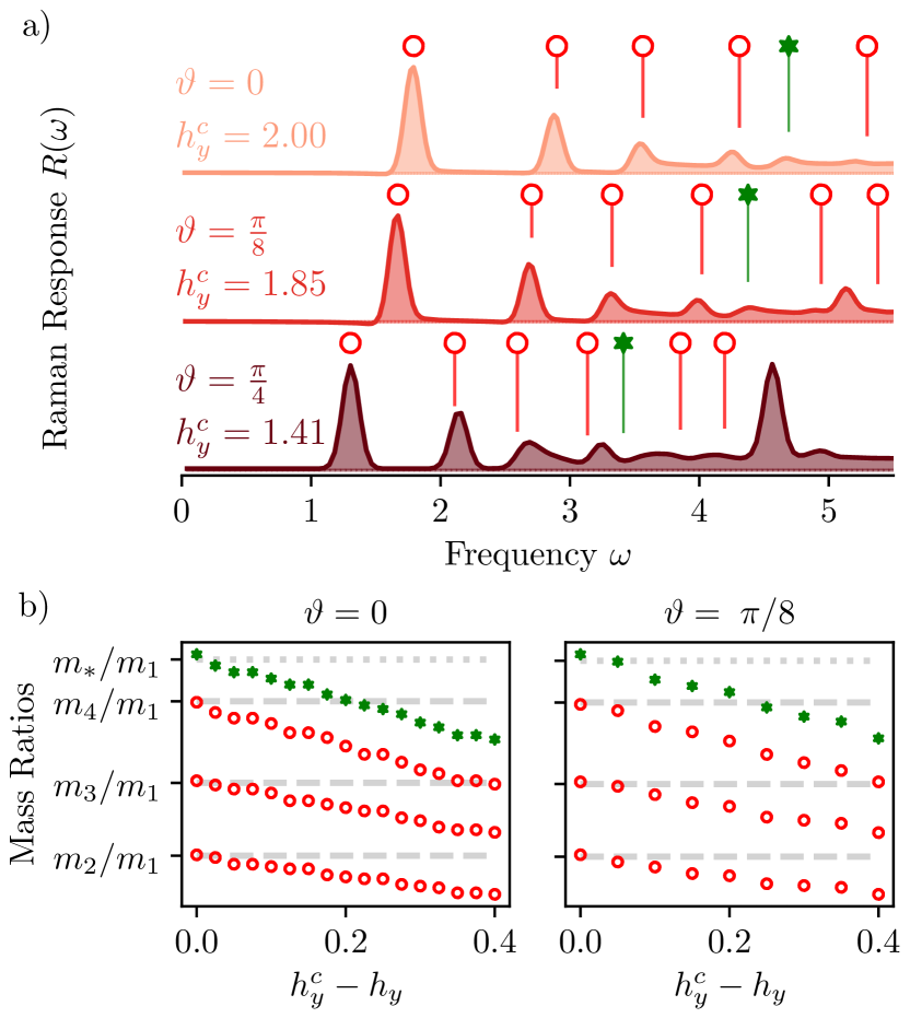
Figure 2: Emergent $E_{8}$ symmetry at Ising quantum criticality. (a) Along the Ising quantum critical line the peaks in the Raman response have the anomalous $E_{8}$ symmetry (red circles and green stars). Deviations from the predicted mass rations arise for high energies, in particular at larger values of the angle $\vartheta$. (b) We illustrate the flow of the bound state masses $(m_{2},m_{3},m_{4})/m_{1}$ (red circles) and the summed mass $m_{*}/m_{1}=(m_{2}+m_{1})/m_{1}$ (green stars) extracted from Raman spectra. The mass ratios converge to the predictions of the $E_{8}$ symmetric field theory as the transverse field $h_{y}$ is tuned to quantum criticality $h_{y}^{c}$. All data has been obtained for the confining field $h_{x}=0.25$ and $h_{z}=0$.

The Raman spectrum is obtained as follows

$$R(\omega)=\int\mathrm{d}t\;e^{i(\omega+E_{0})t}\bra{0}\mathcal{R}e^{-i\mathcal{H}t}\mathcal{R}\ket{0},$$ (5)

where $\ket{0}$ is the ground state and $E_{0}$ denotes its energy. We emphasize that the Raman response couples uniformly to the system and thereby only probes excitations with zero total momentum. This is because the speed of light is much larger than all energy scales of our system. Hence, in order to fulfill energy and momentum conservation, light can only create pairs of excitations with opposite momentum. We use the translational invariance of the excited state $\mathcal{R}\ket{0}$ to efficiently compute the response numerically using iMPS methods [32, 28], see Supplementary Material  for details.

We now focus on a fixed polarization of the light field. Specifically, we set the in-going photon polarization $\hat{e}_{i}$ to be the $-\hat{x}$-direction and the outgoing photon polarization $45^{\circ}$ between the $\hat{e}_{i}$ and $\hat{z}$ directions. With these considerations, the photon projectors only depend on the zigzag angle $\vartheta$ and are given by $P_{e}=\frac{1}{\sqrt{2}}[\cos^{2}({\vartheta}/{2})-{\sin(\vartheta)}/{2}]$ and $P_{o}=\frac{1}{\sqrt{2}}[\cos^{2}({\vartheta}/{2})+{\sin(\vartheta)}/{2}]$. The Raman spectra for vanishing transverse magnetic fields $h_{y}$ and $h_{z}$, different values of $h_{x}$, and zigzag angles $\vartheta\in\{\frac{\pi}{16},\frac{\pi}{8},\frac{\pi}{4}\}$ are shown in Fig. 1 (c). The angle $\vartheta$ is chosen such that the ground state in the absence of the $h_{x}$-field is in the $\hat{x}$-ferromagnetic phase. Our results illustrate how the Raman spectrum crosses over from a continuum in the absence of a longitudinal magnetic field $h_{x}=0$ to a discrete sequence of bound state peaks for increasing $h_{x}$. The results for $h_{x}=0$ are computed analytically and results for finite $h_{x}$ are obtained numerically with iMPS (see Supplementary Material).

To obtain an intuition of the observed discrete peak structure we compare our results to a simple trial wavefunction describing a small number of solitonic domain wall excitations. To construct the basis for this ansatz we start with the ground state configuration of all spins aligned in $\hat{x}$-direction and systematically add pairs of solitons, i.e pairs of domain walls, to the state until we reach a chosen maximal number of domain walls. The projected Hamiltonian restricted to this few soliton subspace is expected to reproduce the low-energy response of the system when the energy cost associated to domain walls is large compared to their kinetic energy. This assumption is valid deep in the ferromagnetic regime and in particular far away from the Ising critical line separating the ordered from the paramagnetic phase.

The peak structure of the Raman spectrum obtained within this few-soliton ansatz captures the exact iMPS results remarkable well for strong longitudinal fields; see Fig. 1 (c). Already the minimum of two domain walls (green stars) capture quantitatively the peak positions for $\vartheta=\frac{\pi}{16}$. However, as the excitation energy for domain walls decreases with increasing $\vartheta$, deviations between the iMPS and the two-soliton ansatz are observed. Including further domain walls significantly improves the accuracy of the predicted peaks (red circles: four domain walls). Hence, the Raman response captures the bound state formation of domain wall excitations and thus serves as a direct probe of domain wall confinement. When approaching the critical point $(\vartheta=\frac{\pi}{2})$ more and more solitons need to be included to reproduce the bound state spectrum. This suggests that the entire spectrum of multi-soliton excitations becomes strongly dressed in the vicinity of the critical point.

Emergent $E_{8}$ symmetry. – The field theory of the Ising quantum critical point has an underlying $E_{8}$ symmetry, which manifests itself in the energies of the bound states in the presence of a weak confinement potential [33, 34]. However, even away from the pristine Ising limit, it has been demonstrated both numerically as well as experimentally that this $E_{8}$ symmetry prevails at low energies, which is an indicator of the underlying Ising quantum critical point [19, 2, 25, 6]. In order to estimate to which extent this signature of quantum criticality can be observed, we compute the Raman response for $\vartheta\in\{0,\frac{\pi}{8},\frac{\pi}{4}\}$ at the corresponding critical values of the transverse field $h_{y}^{c}$ extracted analytically in the absence of other fields. Results corresponding to a weak longitudinal field of $h_{x}=0.25$ are shown in Fig. 2 (a). We compare the results for the Raman response with the mass ratios predicted by $E_{8}$-symmetry for the Ising field theory, given by $(m_{2},m_{3},m_{4},m_{5},m_{6})=(1.618,1.989,2.405,2.956,3.218)m_{1}$ [34]. We observe a well-separated peak structure with excellent agreement close to the Ising point for both zigzag angles $\vartheta=\{0,\frac{\pi}{8}\}$. For larger angles we, however, find deviations from the predicted structure, in particular at high energies. This is expected as perturbations to the bare Ising theory will generically produce subleading corrections that determine the energy regime in which the effective field theory is applicable.

To demonstrate that the observed symmetry is indeed unique to the critical Ising theory we investigate the flow of the mass ratios (red markers) as well as the collective excitation $m_{*}=m_{1}+m_{2}$ (green marker) extracted from the Raman response for different transverse fields $h_{y}$, both at $\vartheta=0$ and $\vartheta=\frac{\pi}{8}$; Fig. 2 (b). The $E_{8}$ mass ratios are only reached when $h_{y}$ approaches $h_{y}^{c}$, and are thus a signature of the critical point.

Characterizing the structure of bound states with Raman scattering. – So far we have investigated the consequences of the magnetic field components $h_{x}$ and $h_{y}$ in the x-polarized FM state. Applying in addition a transverse field $h_{z}$ splits the bound state spectrum, as has been previously detected in experiments [23, 26]. In particular, the hierarchy of bound state peaks in the Raman spectrum splits into three distinct sets of resonances. This peak splitting does not occur for a twisted Kitaev Hamiltonian with a longitudinal field alone. We illustrate the splitting for zigzag angle $\vartheta=\frac{\pi}{16}$ and longitudinal field $h_{x}=0.1$ as well as for $\vartheta=\frac{\pi}{8}$ and $h_{x}=0.25$ in Fig. 3.

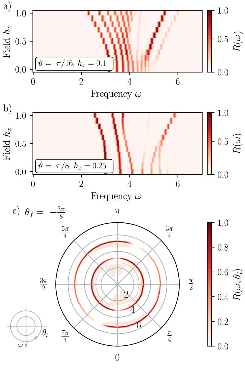
Figure 3: Analyzing the structure of bound states. Transverse field $h_{z}$ dependence of bound state energies for (a) $\vartheta=\frac{\pi}{16},\;h_{x}=0.1$, $h_{y}=0.5$ and (b) $\vartheta=\frac{\pi}{8},\;h_{x}=0.25$, $h_{y}=0.5$. The $h_{z}$ field splits the peak structure into three sets, whose energy either decrease, stays approximately constant, or increase with increasing $h_{z}$. (c) Polar plot of the Raman spectrum as a function of the polarization of incident photons $\theta_{i}$ and fixed outgoing polarization $\theta_{f}=-\frac{3\pi}{8}$. The polarization of the scattered light, allows for selecting antisymmetric and symmetric bound states. The results are obtained for $\vartheta=\frac{\pi}{8},(h_{x},h_{y},h_{z})=(0.1,0.0,0.77)$.

This splitting is a result of different internal symmetries of the excited eigenstates [26] and can therefore be used to explore the internal structure of the bound states. In the x-polarized FM phase for a large transverse $h_{z}$ field the effective Hamiltonian dimerizes. The dimerized bound states factorize into three sets of states, that shift toward lower energies, remain constant, and shift toward higher energies as $h_{z}$ is increased. These states are then symmetric, invariant, and anti-symmetric with respect to a pairwise exchange of even and odd bonds, see Supplementary Material. The flow of the bound state energies with $h_{z}$ field is also seen in the iMPS results of Fig. 3 (a) and (b); for more details see Supplementary Material.

Interestingly, the Raman response allows us to probe the symmetries of the bound states even more directly. Due to the zigzag geometry of the Ising chain, light couples differently to even and odd bonds. When tuning the polarization of the light field, the relative coupling to the bond-centered bound states is tuned. Hence, from the shift of spectral weight one can deduce the structure of the bound state. To demonstrate this effect, we compute the Raman response as a function of the polarization of the incoming photons $\theta_{i}$ for fixed polarization of outgoing photons $\theta_{f}=-\frac{3\pi}{8}$ and $\vartheta=\frac{\pi}{8},(h_{x},h_{y},h_{z})=(0.1,0.,0.77)$; Fig. 3 (c). The spectral peaks are indeed strongly modified when the photon polarization is tuned and individual spectral peaks with different symmetries can be selectively enhanced or suppressed in the Raman response. For a given incoming and outgoing polarization angle, we can predict whether the Raman operator dominantly couples to symmetric, invariant, or anti-symmetric bound states. As a consequence, we can deduce the symmetry of the bound states directly from the Raman spectrum. Moreover, in the pure Ising limit $\vartheta=0$ the bound states are insensitive to the polarization angles. In this limit, the unit cell consists of a single site and even and odd bonds cannot be discerned in light scattering. A dependence of the Raman peaks on the polarization of the scattered light, therefore can be used as a strong signature of effective contributions beyond the pure Ising model.

Discussion & Outlook. – We have demonstrated that Raman light scattering couples to bound states of domain walls in confined Ising spin chains and, hence, can thus be used as a complementary tool to neutron scattering and THz spectroscopy. Remarkably, by tuning the polarization of the scattered light field the internal symmetries of the excitations can be probed. We propose that the polarization dependent scattering intensities can be used to refine the structure of the effective microscopic model.

Our work has focused on the twisted Kitaev chain in a tilted field, which is a minimal description of CoNb2O6. In this system the splitting of the peaks in the Raman spectrum is on the order of $0.1\text{meV}$ [2, 18], which can be resolved with available Raman setups [35, 36, 37, 38]. However, our results go beyond this specific material. For example, recent studies of the quasi one-dimensional antiferromagnet BaCo2V2O8 revealed similar phenomena of mesonic domain-wall bound states. Due to the larger antiferromagnetic interactions, however, the peak splitting of bound states is even on the order of $0.5\text{meV}$ [39, 40, 6, 41]. This renders BaCo2V2O8 a complimentary candidate material for observing bound states of domain walls in inelastic light scattering experiments with even more favorable energy scales. In future work, it will be interesting to study how the selection rules resulting from the polarization of the light fields manifest themselves in other magnetic compounds with confinement.

Acknowledgements. – We thank G. B. Sim, J. Hausschild and F. Pollmann for interesting discussions about the model and details on the numerical methods. We thank R. Hackl and P. v. Loosdrecht for comments on possible experimental implementations. We acknowledge support from the Deutsche Forschungsgemeinschaft (DFG, German Research Foundation) under Germany’s Excellence Strategy–EXC–2111–390814868, TRR 360 – 492547816 and DFG grants No. KN1254/1-2, KN1254/2-1, the European Research Council (ERC) under the European Union’s Horizon 2020 research and innovation programme (grant agreement No. 851161), as well as the Munich Quantum Valley, which is supported by the Bavarian state government with funds from the Hightech Agenda Bayern Plus.

Data and Informations availability. – Data, data analysis, and simulation codes are available upon reasonable request on Zenodo [42].

Supplementary Information
Signatures of Domain-Wall Confinement in Raman Spectroscopy of Ising Spin Chains
Stefan Birnkammer, Johannes Knolle, Michael Knap

1 The Raman Operator

In this section we derive the Raman operator for a generic choice of photon polarizations relative to the sample. Within the Fleury-Loudon theory of Raman spectroscopy, the Raman operator $\mathcal{R}$ is constructed from interactions between two neighboring spins. These are weighted by the projection of the individual photon polarizations onto the bond connecting the spins. Following the notation of the main text, the Raman operator reads

$$\mathcal{R}=\sum_{j=1}^{L}(\hat{\delta}_{j}\cdot\hat{e}_{i})\;\mathcal{H}^{(j)}\;(\hat{\delta}_{j}\cdot\hat{e}_{f})\equiv\sum_{j=1}^{L}P_{j}(\hat{e}_{i},\hat{e}_{f};\vartheta)\;\mathcal{H}^{(j)}$$ (S1)

Here, we denote the unit vectors describing the bond orientation in our zigzag chain by $\hat{\delta_{j}}$. A suitable parameterization of $\hat{\delta_{j}}$ as well as the polarization vectors is given by

$$\hat{\delta_{j}}=\begin{pmatrix}\cos\Big{(}\frac{\vartheta}{2}\Big{)}\\ 0\\ (-1)^{j}\sin\Big{(}\frac{\vartheta}{2}\Big{)}\end{pmatrix} \hat{e}_{i/f}=\begin{pmatrix}\sin(\theta_{i/f})\cos(\phi_{i/f})\\ \sin(\theta_{i/f})\sin(\phi_{i/f})\\ \cos(\theta_{i/f})\end{pmatrix}.$$ (S2)

With this convention the projectors $P_{j}(\hat{e}_{i},\hat{e}_{f};\vartheta)$ included in Eq. (S1) assume two distinct values for even and odd bonds, respectively

$$P_{e}(\hat{e}_{i},\hat{e}_{f}) =\Big{[}\cos\Big{(}\frac{\vartheta}{2}\Big{)}\sin(\theta_{i})\cos(\phi_{i})+\sin\Big{(}\frac{\vartheta}{2}\Big{)}\cos(\theta_{i})\Big{]}\times\Big{[}\cos\Big{(}\frac{\vartheta}{2}\Big{)}\sin(\theta_{f})\cos(\phi_{f})+\sin\Big{(}\frac{\vartheta}{2}\Big{)}\cos(\theta_{f})\Big{]}$$ (S3)

$$P_{o}(\hat{e}_{i},\hat{e}_{f}) =\Big{[}\cos\Big{(}\frac{\vartheta}{2}\Big{)}\sin(\theta_{i})\cos(\phi_{i})-\sin\Big{(}\frac{\vartheta}{2}\Big{)}\cos(\theta_{i})\Big{]}\times\Big{[}\cos\Big{(}\frac{\vartheta}{2}\Big{)}\sin(\theta_{f})\cos(\phi_{f})-\sin\Big{(}\frac{\vartheta}{2}\Big{)}\cos(\theta_{f})\Big{]}.$$ (S4)

Thus the Raman operator takes the simple functional form denoted in Eq. (4) of the main text. Considering only photon scattering processes in the plane spanned by $\hat{\delta_{1}}$ and $\hat{\delta_{2}}$, moreover, fixes $\phi_{i}=\phi_{f}=0$. In general, we find that the Raman operator inherits the two-site unit cell of the Hamiltonian with local contributions $\mathcal{R}^{(j)}$ acting on three spins

$$\mathcal{R}=\sum_{j=1}^{L/2}\Big{[}P_{e}(\hat{e}_{i},\hat{e}_{f})\mathcal{H}^{(2j)}+P_{o}(\hat{e}_{i},\hat{e}_{f})\mathcal{H}^{(2j+1)}\Big{]}\equiv\sum_{j=1}^{L/2}\mathcal{R}^{(j)}.$$ (S5)

2 Polarization Dependence of Raman Responses

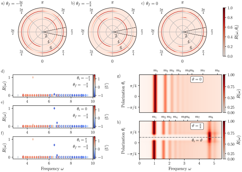
Figure S1: Symmetry Selection of Peaks (a) - (c) Raman response obtained from a few domain wall ansatz as a function of ingoing photon polarization $\theta_{i}$ for outgoing polarization angles $\theta_{f}\in\{-\frac{3\pi}{8},-\frac{\pi}{8},0\}$ and system parameters $\vartheta=\frac{\pi}{8},(h_{x},h_{y},h_{z})=(0.1,0.,0.77)$ showing the different selection rules for high and low energy bound states. (d) - (f) The differences between both sets of excitations can be understood from symmetry properties of the eigenstates the pairwise exchange of even and odd bonds $U$. We find symmetric eigenstates to determine the low energy response (red markers) while the high energy spectrum is governed by antisymmetric states (blue markers). (g,h) We, moreover, investigate the role of ingoing photon polarization at quantum criticality in iMPS simulations for in-plane scattering ($\phi_{i}=\phi_{f}=0$) while keeping the outgoing photon polarization $\theta_{f}=-\frac{3\pi}{8}$ fixed. (g) For the pure Ising limit $(\vartheta=0.)$ at quantum criticality $(h_{y},h_{z})=(2.0,0.0)$ we detect a polarization independent spectrum exhibiting the field theoretically predicted $E_{8}$-symmetry as we apply a longitudinal field $h_{x}=0.1$, as expected for systems with a single-site unit cell. Changes in the photon polarization only result in amplitude modulations of the Raman response. (h) Away from the Ising limit, polarization control allows to tune the values $P_{e}$ and $P_{o}$ enabling a selection of excitations according to their internal symmetries. For $\vartheta=\frac{\pi}{8}$ and critical magnetic field $h_{y}^{c}=1.85$ we detect a set of peaks whose amplitude can be enhanced for photon polarization $\theta_{i}=\vartheta$. The latter violate the predictions for an $E_{8}$-symmetric spectrum and can be taken as an experimentally accessible fingerprint for non-Ising contributions to the Hamiltonian.

Having obtained the general expression for the Raman operator, Eq. (S5), we now discuss some situations, where the polarization of incoming and outgoing photons can indeed influence the measured response in a nontrivial way. A detailed study of the Raman spectra obtained from the two-domain wall state as a function of the scattered light polarizations are shown in Fig. S1 (a) - (c). We find that the two-domain wall approximation is able to qualitatively reproduce the iMPS results of Fig. 3 (c) of the main text. Moreover, we will now discuss the internal structure of the bound states by constructing an effective model for the domain wall dynamics, following Ref. [26]. To this end, we label the two distinct types of domain walls appearing in our system as $\ket{j}_{L}=\ket{\dots\uparrow\uparrow_{j}\downarrow_{j+1}\downarrow\dots}$ and $\ket{j}_{R}=\ket{\dots\downarrow\downarrow_{j}\uparrow_{j+1}\uparrow\dots}$. The dynamics governed by Hamiltonian (1) for $h_{x}=0$ within a fixed domain wall sector is given by

$$\mathcal{H}\ket{j}_{L}\mapsto-\sin^{2}\Big{(}\frac{\vartheta}{2}\Big{)}\Big{[}\ket{j-2}_{L}+\ket{j+2}_{L}\Big{]}+\Big{[}\Delta_{L}\sin(\vartheta)-i\frac{h_{y}}{2}-\frac{h_{z}}{2}\Big{]}\ket{j+1}_{L}+\Big{[}-\Delta_{L}\sin(\vartheta)+i\frac{h_{y}}{2}-\frac{h_{z}}{2}\Big{]}\ket{j-1}_{L}$$ (S6)

where we introduced $\Delta_{L}=\bra{j}_{L}\sigma_{j-1}^{x}-\sigma_{j+1}^{x}\ket{j}_{L}/2=1$. A similar expression can be obtained for $\ket{j}_{R}$ with $\Delta_{R}=-1$, instead. In the following, we will consider small values of $\vartheta\ll 1$ allowing us to neglect the next-nearest neighbor terms contained in Eq. (S6) at leading order. Moreover, we consider only in-plane magnetic fields of our quasi one-dimensional system, i.e. set $h_{y}=0$. When selecting the specific field of $h_{z}=2\sin(\vartheta)$, the $L$ soliton is only allowed to move within a single unit cell $p$ with bonds $(2p-1,2p)$ and the $R$ soliton can only hop between neighboring unit cells connected by bonds $(2p,2p+1)$. The corresponding eigenstates for the single domain wall problem are given by plane wave states built from (anti-)symmetric superpositions in the disconnected two-bond systems

$$\ket{p}_{L}^{\pm} =\frac{1}{\sqrt{2}}\big{[}\ket{2p-1}_{L}\pm\ket{2p}_{L}\big{]} \ket{p}_{R}^{\pm} =\frac{1}{\sqrt{2}}\big{[}\ket{2p}_{R}\pm\ket{2p+1}_{R}\big{]}.$$ (S7)

Solutions for the two-domain wall problem can be constructed as bound states of two domain walls with given distance

$$\ket{n,k}^{\pm} =\frac{1}{\sqrt{N}}\sum_{p}e^{i\frac{k}{2}(2p+n)}\ket{p}_{L}^{\pm}\otimes\ket{p+n}_{R}^{\pm}$$

$$\ket{n,k}^{0}_{\pm} =\frac{1}{\sqrt{2N}}\sum_{p}e^{i\frac{k}{2}(2p+n)}\Big{[}\ket{p}_{L}^{+}\otimes\ket{p+n}_{R}^{-}\pm\ket{p}_{L}^{-}\otimes\ket{p+n}_{R}^{+}\Big{]}\quad\text{with}\quad n\geq 1,$$ (S8)

where $N$ denotes the number of unit cells in the system. The associated energies are given by $\omega_{\pm}=4\cos^{2}(\frac{\vartheta}{2})\mp h_{z}$ and $\omega_{0}=4\cos^{2}(\frac{\vartheta}{2})$. With that one can understand the trends of the bound state energies as a function of $h_{z}$ observed in the spectra of Fig. 3; see also Ref. [26]. For $n=0$, corresponding to neighboring solitons, we have to additionally take into account a hardcore constraint prohibiting the solitons to occupy the same bond. As a result the eigenstates get altered

$$\ket{\epsilon,k}^{\pm} =\frac{1}{\sqrt{N}}\sum_{p}e^{ikp}\Big{[}\ket{2p-1}_{L}\otimes\ket{2p}_{R}+\ket{2p}_{L}\otimes\ket{2p+1}_{R}\pm\sqrt{2}\ket{2p-1}_{L}\otimes\ket{2p+1}_{R}\Big{]}$$

$$\ket{\epsilon,k}^{0} =\frac{1}{\sqrt{2N}}\sum_{p}e^{ikp}\Big{[}\ket{2p-1}_{L}\otimes\ket{2p}_{R}-\ket{2p}_{L}\otimes\ket{2p+1}_{R}\Big{]}$$ (S9)

with corresponding eigenenergies of $\epsilon_{\pm}=4\cos^{2}(\frac{\vartheta}{2})\mp\sqrt{2}h_{z}$ and $\epsilon_{0}=4\cos^{2}(\frac{\vartheta}{2})$. It is worth noting that the large degeneracy in eigenenergies found here, will be lifted by finite longitudinal fields $h_{x}$ penalizing large distances between the domain walls.

We have now understood the flow of eigenenergies as a function of the field $h_{z}$. As a next step we want to analyze their internal wave function. To this end, we consider the pairwise exchange of even and odd bonds

$$U=\sum_{p}\Big{[}\ket{2p-1}_{L}\bra{2p}_{L}+\ket{2p-1}_{R}\bra{2p}_{R}+\text{h.c.}\Big{]}.$$ (S10)

One finds, that $\ket{n,k}^{+}$ and $\ket{\epsilon,k}^{+}$ have positive, $\ket{n,k}^{-}$ and $\ket{\epsilon,k}^{-}$ negative, and $\ket{n,k}_{0}^{\pm}$, $\ket{\epsilon,k}^{0}$ have vanishing expectation values of $U$. In our few-soliton approach we can test the predicted symmetry classification of high and low energy peaks for the eigenstates; Fig. S1 (d) - (f). For different $\theta_{i}$ values we can selectively excite symmetric (d) or antisymmetric (e) eigenstates or both (f). We indeed resolve a splitting of the measured Raman spectrum into symmetric low-energy and antiysmmetric high-energy modes.

As a next step we investigate the polarization dependence of the Raman response at quantum criticality. In the main text we emphasized that an emergent $E_{8}$ symmetry predicted for the spectrum of a confined Ising theory can be resolved using Raman techniques. As shown in Fig. 2 we do, however, find corrections to the expected scaling behavior of excitations at high energies when considering finite values of the zigzag angle $\vartheta$. A more detailed investigation of the excitation structure for different values of the incoming photon polarization is shown in Fig. S1 (e). For the pure Ising case all observed resonances follow the predicted $E_{8}$-symmetry. Changes in the photon polarization are only reflected in the total amplitude of the Raman response signal, not leading to a modification of individual excitations, as expected for a system with a single-site unit cell. Considering, however, finite values of $\vartheta=\frac{\pi}{8}$, for example, we observe a resonance that violates the $E_{8}$ Ising scaling of bound state peaks. Moreover, the scattering intensity of solely these peaks can be modified by the right choice of the polarization $\theta_{i}$, see Fig. S1 (f). The detected high-energy peak structure can hence be attributed to Kitaev contributions to the Hamiltonian (1). In this sense the control of photon polarization in Raman spectroscopy can be used to probe excitations violating the predictions of a confined Ising theory at criticality. The latter can serve as markers for Kitaev contributions in the microscopic Hamiltonian.

3 Complexity of Excitations Near Quantum Criticality

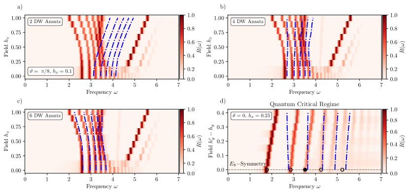
Figure S2: Breakdown of the few-soliton ansatz near quantum criticality. We compare numerically exact iMPS simulations (color plot) and the few-soliton ansatz (blue dash-dotted line) with up to (a) 2, (b) 4 and (c) 6 domain walls for a system with 32 sites. We show the spectrum for $\vartheta=\frac{\pi}{8}$, $h_{x}=0.1,h_{y}=0.5$ and tune $h_{z}$ field. In contrast to the results of Fig. 1 (c), which have been obtained in the perturbative regime, we find that the spectra near criticality deviate from the few-soliton ansatz, even for the largest number of domain walls that we consider, indicating that the bound states possess a more complex structure. (d) In the vicinity of the critical point in the pure Ising case ($\vartheta=0,h_{z}=0,h_{x}=0.25$) all domain wall sectors are expected to contribute to the response, inevitably leading to a breakdown of the few domain-wall ansatz as illustrated for the 6 domain wall case (blue dash-dotted line).

Here, we study the validity regime of the few domain wall ansatz. The comparison between tensor network results and few-soliton ansatz in the subspace of two and four solitons is discussed in the main text for the perturbative regime; Fig. 1 (c). This simple few domain-wall ansatz is only valid deep in the ferromagnetic phase where the excitation gap for domain walls is the dominant scale, i.e., $\vartheta\to 0$ and $h_{y}\ll h_{y}^{c}$. Considering, in contrast parameters closer to the critical regime as shown in Fig. S2 (a) - (c) we find that the two domain-wall ansatz cannot reproduce the qualitative trends obtained from tensor network simulations. We investigate the flow of the peak structure as we tune the transverse field $h_{z}$ for values of $\vartheta=\frac{\pi}{8},h_{y}=0.5$ and $h_{x}=0.1$. Besides a disagreement in energy we find increasing bound state masses for both the two and four domain-wall ansatz (blue dash-dotted lines) as $h_{z}$ is increased, whereas iMPS shows the opposite trend. Considering an ansatz involving 6 domain walls captures the right trend, however energies still disagree in particular for large fields $h_{z}$. This indicates a more complicated structure of excitations going beyond the simple two soliton bound states. Following up on this prediction we benchmark the Raman response of 6 domain wall ansatz at quantum criticality of the Ising theory ($\vartheta=0,h_{z}=0,h_{x}=0.25$); Fig. S2 (d). When tuning the transverse field $h_{y}$ to the quantum critical point $h_{y}^{c}=2.0$, clear deviations from the predicted $E_{8}$-symmetry are found (black markers). By contrast, iMPS correctly reproduces the scaling of the field theory. This again shows that the confined states possess a complex structure at the quantum critical point.

4 Raman Response in the Integrable Regime

1 Spectrum of the Exaclty Solvable Model

In the presence of the transverse $h_{y}$ field only, our system is integrable. We now analytically compute the Raman response for this regime. On the one hand, we will use these results to quantitatively determine the phase boundaries sketched in Fig. 1 (b). On the other hand, we can use them to benchmark the accuracy of our numerical results obtained with iMPS. We emphasize already now that due to the absence of confinement and the fast speed of excitations, this integrable case is actually the most difficult case for iMPS.

For the analytical solution we make use of a Jordan-Wigner transformation and map the spin model to dual fermions. The latter can be solved by a Bogoliubov transformation, which directly allows us to compute the Raman response. We define the Jordan-Wigner mapping in y-direction to end up with a theory of well defined fermion parity

$$\sigma_{i}^{y} =2c_{i}^{\dagger}c_{i}-1 \sigma_{i}^{x} =\prod_{j<i}(1-2c_{j}^{\dagger}c_{j})(c_{i}+c_{i}^{\dagger}) \sigma_{i}^{z} =-i\prod_{j<i}(1-2c_{j}^{\dagger}c_{j})(c_{i}-c_{i}^{\dagger}).$$ (S11)

Inserting this transformation in the Hamiltonian (1) for $h_{x}=h_{z}=0$ we find

$$\mathcal{H}(\vartheta) =-\sum_{j=1}^{L}\Big{[}c_{j}^{\dagger}c_{j+1}+\Big{(}\cos(\vartheta)+i(-1)^{j}\sin(\vartheta)\Big{)}c_{j}^{\dagger}c_{j+1}^{\dagger}+\text{h.c.}\Big{]}-\frac{h_{y}}{2}\sum_{j=1}^{L}\Big{[}2c_{j}^{\dagger}c_{j}-1\Big{]}$$

$$=-\sum_{j=1}^{L/2}\Big{[}b_{j}^{\dagger}a_{j}+a_{j}^{\dagger}b_{j+1}+e^{i\vartheta}b_{j}^{\dagger}a_{j}^{\dagger}+e^{-i\vartheta}a_{j}^{\dagger}b_{j+1}^{\dagger}+\text{h.c.}\Big{]}-\frac{h_{y}}{2}\sum_{j=1}^{L/2}\Big{[}2a_{j}^{\dagger}a_{j}+2b_{j}^{\dagger}b_{j}-2\Big{]}.$$ (S12)

In the last line we have introduced operators for the unit cell on odd ($a_{j}=c_{2j+1}$) and even ($b_{j}=c_{2j}$) sites. Using the translational invariance of the two-site unit cell, the Fourier transformation is given by

$$a_{k} =\sqrt{\frac{2}{L}}\sum_{j=1}^{L/2}e^{ikj}a_{j} b_{k} =\sqrt{\frac{2}{L}}\sum_{j=1}^{L/2}e^{ikj}b_{j}.$$ (S13)

Then the momentum space representation of $\mathcal{H}$ reads

$$\mathcal{H}(\vartheta) =-\sum_{k}\Big{[}e^{i\vartheta}b_{k}^{\dagger}a_{-k}^{\dagger}+b_{k}^{\dagger}a_{k}+e^{-i(\vartheta-k)}a_{-k}^{\dagger}b_{k}^{\dagger}+e^{-ik}a_{k}^{\dagger}b_{k}+\text{h.c.}\Big{]}-\frac{h_{y}}{2}\sum_{j}\Big{[}2a_{k}^{\dagger}a_{k}+2b_{k}^{\dagger}b_{k}\Big{]}-\frac{h_{y}}{2}L$$

$$\equiv-\sum_{k}\Big{[}A(k)b_{k}^{\dagger}a_{k}+A(k)^{*}a_{k}^{\dagger}b_{k}+B(k,\vartheta)b_{k}^{\dagger}a_{-k}^{\dagger}+B(k,\vartheta)^{*}a_{-k}b_{k}\Big{]}+\mathcal{C},$$ (S14)

where $A(k)=1+e^{ik}$ and $B(k,\vartheta)=e^{i\vartheta}-e^{i(k-\vartheta)}=\cos(\vartheta)(1-e^{ik})+i\sin(\vartheta)(1+e^{ik})\equiv B_{1}(k,\vartheta)+B_{2}(k,\vartheta)$ depend on the momentum and the zigzag angle $\vartheta$. We also introduced a variable accounting for the overall constant factor $\mathcal{C}=-\frac{K}{2}h_{y}L$. Additionally we find a parity symmetry reflected in $A(k)=A(-k)^{*}$.
We can symmetrize the expression to bring it to conventional Bogoliubov-deGennes form using the spinor notation $\psi_{k}^{\dagger}=(a_{k}^{\dagger},a_{-k},b_{k}^{\dagger},b_{-k})$

$$\mathcal{H}_{BdG}(\vartheta)=-\frac{1}{2}\sum_{k}\psi_{k}^{\dagger}\;\Gamma(k;\vartheta)\;\psi_{k}$$ (S15)

with the geometric coupling matrix

$$\Gamma(k,\vartheta)=\begin{pmatrix}h_{y}&0&A(k)^{*}&-B(-k,\vartheta)\\ 0&-h_{y}&B(k,\vartheta)^{*}&-A(k)^{*}\\ A(k)&B(k,\vartheta)&h_{y}&0\\ -B(-k,\vartheta)^{*}&-A(k)&0&-h_{y}\end{pmatrix}.$$ (S16)

After diagonalizing the Hamiltonian (S15) using the eigenmodes of $\Gamma(k,\vartheta)$ we find

$$\mathcal{H}_{BdG}(\vartheta)=\sum_{k}\Big{[}\gamma_{k}\Big{(}\alpha_{k}^{\dagger}\alpha_{k}-\frac{1}{2}\Big{)}+\rho_{k}\Big{(}\beta_{k}^{\dagger}\beta_{k}-\frac{1}{2}\Big{)}\Big{]},$$ (S17)

where $\alpha_{k},\beta_{k}$ are the operators contained in the diagonalizing Nambu spinor $\phi_{k}^{\dagger}=(\alpha_{k}^{\dagger},\alpha_{-k},\beta_{k}^{\dagger},\beta_{-k})$ defined via the unitary transformation $\Lambda(k,\vartheta)$ diagonalizing $\Gamma(k,\vartheta)$

$$\Lambda(k,\vartheta)^{-1}\Gamma(k,\vartheta)\Lambda(k,\vartheta) =\text{diag}(\gamma_{k},-\gamma_{-k},\rho_{k},-\rho_{-k}) \phi_{k}^{\dagger} =\psi_{k}^{\dagger}\Lambda(k,\vartheta).$$ (S18)

The eigenenergies thereby relate to the functions $A(k)$ and $B(k,\vartheta)$ as

$$\gamma_{k} =\sqrt{h_{y}^{2}+\xi_{k}-\sqrt{4\lambda_{k}h_{y}^{2}+\xi_{k}^{2}-\eta_{k}^{2}}} \rho_{k} =\sqrt{h_{y}^{2}+\xi_{k}+\sqrt{4\lambda_{k}h_{y}^{2}+\xi_{k}^{2}-\eta_{k}^{2}}}$$ (S19)

with

$$\xi_{k} =|A(k)|^{2}+|B_{1}(k)|^{2}+|B_{2}(k)|^{2} \eta_{k} =|A(k)^{2}-B_{1}(k)^{2}+B_{2}(k)^{2}| \lambda_{k} =|A(k)|^{2}=2-2\cos(k).$$ (S20)

The dispersion denoted in (S19) reduces in the limiting case of $\vartheta=0$ to the well-known Ising dispersion for a transverse magnetic field $h_{y}$

$$\gamma_{k}\rvert_{\vartheta=0}=2\sqrt{1+\Big{(}\frac{h_{y}}{2}\Big{)}^{2}\pm h_{y}\cos\Big{(}\frac{k}{2}\Big{)}}.$$ (S21)

For the pure Kitaev case ($\vartheta=\pi/2$) we find

$$\gamma_{k}\rvert_{\vartheta=\frac{\pi}{2}}=\sqrt{8\cos^{2}\Big{(}\frac{k}{2}\Big{)}+h_{y}^{2}\pm 4\Big{|}\cos\Big{(}\frac{k}{2}\Big{)}\Big{|}\sqrt{h_{y}^{2}+4\cos^{2}\Big{(}\frac{k}{2}\Big{)}}}$$ (S22)

including the zero mode for the Kitaev model for the minus branch in the case of $h_{y}=0$. The quantitative phase diagram resulting from the dispersion (S19) is shown in Fig. S3 (a).

2 Raman Response of the Dual Fermionic Theory

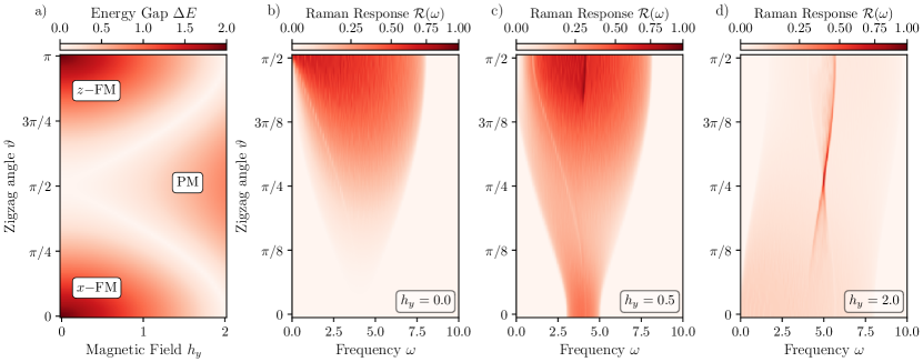
Figure S3: Analytical results for phase diagram and Raman response in the integrable limit. (a) We show the analytical result for the energy gap $\Delta E$ for the integrable regime $h_{x}=h_{z}=0$ as a function of zigzag angle $\vartheta$ and transverse field $h_{y}$. There is an Ising critical line separating the two ferromagnetic phases from a magnetically disordered paramagnetic phase. (b) - (d) Analytical predictions for the Raman response $R(\omega)$ for different values of $h_{y}$ are shown as a function of frequency $\omega$ and zigzag angle $\vartheta$. While in the FM phase the Raman response is dominated by the two-domain wall continuum, the spectrum of the PM is dominated by scattering processes involving the flat band of the Kitaev model, associated with a divergent density of states.

To evaluate the Raman spectra, the Raman operator has to be expressed in the diagonal basis of the Hamiltonian Eq. (S17). First, we rewrite the expression for the Raman operator of Eq. (S5) in the fermionic basis

$$\mathcal{R}(\vartheta)=\sum_{j}^{L/2}\Big{[}P_{o}(\hat{e}_{i},\hat{e}_{f};\vartheta)\big{(}b_{j}^{\dagger}a_{j}^{\dagger}e^{i\vartheta}+b_{j}^{\dagger}a_{j}+\text{h.c.}\big{)}+P_{e}(\hat{e}_{i},\hat{e}_{f};\vartheta)\big{(}a_{j}^{\dagger}b_{j+1}^{\dagger}e^{-i\vartheta}+a_{j}^{\dagger}b_{j+1}+\text{h.c.}\big{)}\Big{]}.$$ (S23)

Transforming the expression into momentum space we end up with

$$\mathcal{R}(\vartheta)=\sum_{k}\Big{[}\big{(}P_{o}(\hat{e}_{i},\hat{e}_{f};\vartheta)+P_{e}(\hat{e}_{i},\hat{e}_{f};\vartheta)e^{ik}\big{)}b_{k}^{\dagger}a_{k}+\big{(}P_{o}(\hat{e}_{i},\hat{e}_{f};\vartheta)e^{i\vartheta}-P_{e}(\hat{e}_{i},\hat{e}_{f};\vartheta)e^{i(k-\vartheta)}\big{)}b_{k}^{\dagger}a_{-k}^{\dagger}+\text{h.c.}\Big{]}.$$ (S24)

This is similar to the result we obtained when diagonalizing the Hamiltonnian with the minor difference that we have to include projectors for the photon directions into the definitions of $A(k)$ and $B(k,\vartheta)$

$$\tilde{A}(k) =P_{o}(\hat{e}_{i},\hat{e}_{f};\vartheta)+P_{e}(\hat{e}_{i},\hat{e}_{f};\vartheta)e^{ik} \tilde{B}(k,\vartheta) =P_{o}(\hat{e}_{i},\hat{e}_{f};\vartheta)e^{i\vartheta}-P_{e}(\hat{e}_{i},\hat{e}_{f};\vartheta)e^{i(k-\vartheta)}$$ (S25)

In this notation, the Raman operator takes the form

$$\mathcal{R}(\vartheta)=\frac{1}{2}\sum_{k}\psi^{\dagger}_{k}\;\tilde{\Gamma}(k;\vartheta,\hat{e}_{i},\hat{e}_{f})\;\psi_{k}$$ (S26)

and $\tilde{\Gamma}(k;\vartheta,\hat{e}_{i},\hat{e}_{f})$ having fundamentally the same form as the $\Gamma(k;\vartheta)$ coupling matrix of the Hamiltonian with new coefficients $A(k)\rightarrow\tilde{A}(k),B(k,\vartheta)\rightarrow\tilde{B}(k,\vartheta)$

$$\tilde{\Gamma}(k;\vartheta,\hat{e}_{i},\hat{e}_{f})=\begin{pmatrix}0&0&\tilde{A}(k)^{*}&-\tilde{B}(-k,\vartheta)\\ 0&0&\tilde{B}(k,\vartheta)^{*}&-\tilde{A}(k)^{*}\\ \tilde{A}(k)&\tilde{B}(k,\vartheta)&0&0\\ -\tilde{B}(-k,\vartheta)^{*}&-\tilde{A}(k)&0\end{pmatrix}.$$ (S27)

In the diagonal basis of $\mathcal{H}$ this changes according to the basis change $\Lambda(k;\vartheta)$ resulting from the Bogoliubov transformation

$$\mathcal{R}(\vartheta)=\sum_{k}\phi^{\dagger}_{k}\;\tilde{D}(k;\vartheta,\hat{e}_{i},\hat{e}_{f})\;\phi_{k}$$ (S28)

with $\tilde{D}(k;\vartheta,\hat{e}_{i},\hat{e}_{f})=\Lambda(k;\vartheta)^{\dagger}\tilde{\Gamma}(k;\vartheta,\hat{e}_{i},\hat{e}_{f})\Lambda(k;\vartheta)$.
Eq. (S28) allows us to evaluate the Raman response for a generic eigenstate of the exactly solvable model. Here we are, however, primarily interested in the ground state response of the system and compute

$$R(\omega) =\int\mathrm{d}t\;e^{i(\omega+E_{0})t}\bra{0}\mathcal{R}e^{-i\mathcal{H}t}\mathcal{R}\ket{0}$$ (S29)

$$=\int\mathrm{d}t\;e^{i(\omega+E_{0})t}\sum_{k,q}\tilde{D}_{\alpha\beta}(k;\vartheta,\hat{e}_{i},\hat{e}_{f})\tilde{D}_{\gamma\delta}(q;\vartheta,\hat{e}_{i},\hat{e}_{f})\bra{0}\phi_{k,\alpha}^{\dagger}\phi_{k,\beta}e^{-i\mathcal{H}t}\phi_{q,\gamma}^{\dagger}\phi_{q,\delta}\ket{0}.$$ (S30)

For the finite frequency response only the connected diagrams contribute, which are related with processes involving two excitations that can propagate in time. Analytical results for $R(\omega)$ at different values of the transverse field $h_{y}$ are shown in Fig. S3 (b) - (d).

5 Details on Numerical Methods

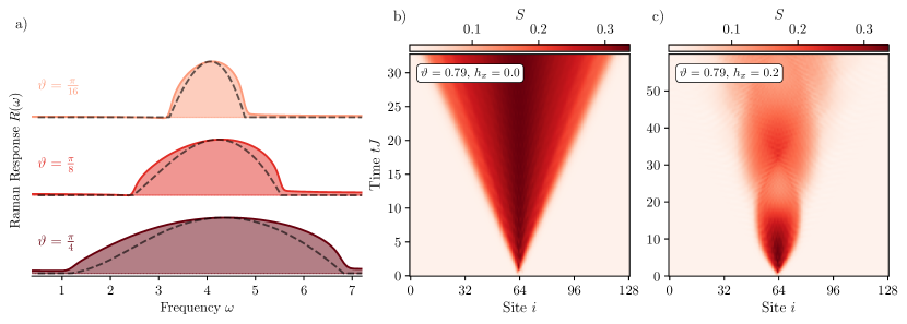
Figure S4: Raman response obtained from iMPS in the analytically solvable limit. (a) We benchmark the results obtained from the iMPS approach (colored areas) with analytical predictions (gray dashed lines) for different values of $\vartheta\in\{\frac{\pi}{16},\frac{\pi}{8},\frac{\pi}{4}\}$ and $h_{x}=h_{y}=h_{z}=0.$. Within our simulations, using a unit cell of $L=128$ sites, we find the energy range of excitations as well as the frequency for the largest Raman response to be well reproduced by iMPS. Qualitative differences, however, are evident in the functional form of the spectral response. This discrepancy is a result of the short simulation times we can reach due to fast entanglement growth in the integrable regime. (b) The lightcone spreading of entanglement after applying the local Raman density in the center of the unit cell in the absence of a longitudinal field limits the maximal simulation times to $tJ\sim 30$ for the unit cell size $L=128$. (c) In presence of a longitudinal field entanglement growth is drastically reduced due to the confining potential between pairs of excited fermions. As a consequence, our simulations yield accurate results up to at least double as long times of $tJ\sim 60$ as demonstrated for the example of $\vartheta=\frac{\pi}{4},h_{x}=0.2$ and $h_{y}=h_{z}=0$.

1 Raman Response from iMPS simulations

For finite systems with confinement, single-domain wall excitations can be stabilized in the vicinity of the boundaries. To avoid these artifacts we develop infinite system size matrix product states (iMPS). We use the TeNPy library as a basic framework for our simulations [43]. Our approach is conceptually similar to earlier works [32, 28] and consists of the following steps:

1. Compute the ground state $\ket{0}$ with energy $E_{0}$ of the system for given parameters of Hamiltonian (1) using the iDMRG algorithm.

2. Blow-up the tensor to $L$.

3. Compute the set of states $I=\{\mathcal{R}^{(j)}\ket{0}\}_{1\leq j<L}$ obtained from applying the local Raman operator $\mathcal{R}^{(j)}$ defined in Eq. (S5) to site $j$ of the iMPS.

4. Perform a time evolution of the specific state $\mathcal{R}^{(L/2)}\ket{0}$ using the iTEBD algorithm.

5. Calculate the gauge-fixed overlap between the time evolved state and all states of $I$ by calculating the dominant eigenvalue of the transfer matrix within the spatial window of size $L$, i.e., compute $C^{(j)}(t)\equiv e^{iE_{0}t}\bra{0}\mathcal{R}^{(j)}e^{-i\mathcal{H}t}\mathcal{R}^{(L/2)}\ket{0}$ for all values of $j$ [19, 32, 28].

6. Making use of the translational invariance manifest in the iMPS formalism compute $R(t)=L\sum_{j=1}^{L}C^{(j)}(t)$.

In the last step we have used that the tensors in the iMPS are translational invariant. This is what ultimately allows us to efficiently compute the Raman response probing the zero momentum response of the system. We obtain converged results in the regime of confinement for bond dimensions of $\chi=200$ and all data shown in this manuscript is obtained for $\chi=400$. In fact the most challenging regime for the iMPS method is the free fermion case in absence of a confining field, as the excitations created by the Raman operator can travel with a high velocity through the systems. In that limit, we indeed find differences between analytical predictions and numerical results, as shown in Fig. S4 (a). Although, the total energy regime for excitations are captured well, the iMPS results cannot reproduce the precise form of the response due to the comparatively short accessible simulations times. Ballistic spreading of entanglement limits the times up to which we can simulate with a given unit cell of length $L$. Once a longitudinal field is applied, the spectral response stays confined to a finite region of space for long times, reducing the effective growth of entanglement. The behavior of the entanglement growth without and with an applied longitudinal field is shown in Fig. S4 (b) and (c).

2 Few Domain-Wall Ansatz

To obtain physical insights into the numerical results obtained from tensor network methods, we have also implemented a few domain wall ansatz. This approach projects the Hilbert space to a maximal domain wall number and then uses exact diagonalization on a finite system with periodic boundary conditions. Concretely, we construct a basis for the Hilbert space starting from the ferromagnetic configurations and successively adding pairs of domain walls to the states. It is worth pointing out that this construction explicitly avoids configurations of odd soliton number, which for the confined phases would lead to irrelevant high-energetic excitations. With this procedure the full low energy Hilbert space can be spanned. In practice we stop the construction with $N$ domain walls and project the model into this subspace ending up with a Hamiltonian $\mathcal{H}_{N}$ [44].
This approach has two main advantages; first and foremost it enables us to simulate exactly comparatively large systems. The dominant contribution to the subspace results from the sector of largest domain wall number $N$, which scales with system size as $\propto\binom{L}{N}$. Comparing this to the exponential scaling of the full Hilbert space ($\propto 2^{L}$) we can thus simulate much larger values of $L$ with comparable computational resources. Secondly, stepwise increasing the number of solitons taken into account in our simulation can give us additional information about the nature of low-energy quasiparticles in our system. This is also discussed in the main text in Fig. 1 (c). There, we find that for small values of $\vartheta=\frac{\pi}{16}$ already 2 domain walls accurately reproduce the peak structure of the iMPS calculations, indicating that bound states of only two solitons describe the low-energy response of the model. For larger values of $\vartheta=\frac{\pi}{4}$ contributions from higher domain wall number sectors are required. The true bound states are thus dressed excitations. When approaching quantum criticality the structure of the confined bound states becomes increasingly complex as discussed in Sec. 3.

References

- Lake et al. [2010] B. Lake, A. M. Tsvelik, S. Notbohm, D. Alan Tennant, T. G. Perring, M. Reehuis, C. Sekar, G. Krabbes, and B. Büchner, Confinement of fractional quantum number particles in a condensed-matter system, Nature Physics 6, 50 (2010).
- Coldea et al. [2011] R. Coldea, D. A. Tennant, E. M. Wheeler, E. Wawrzynska, D. Prabhakaran, M. Telling, K. Habicht, P. Smeibidl, and K. Kiefer, Quantum criticality in an ising chain: experimental evidence for emergent symmetry, Science 327, 177 (2010) (2011).
- Wang et al. [2015] Z. Wang, M. Schmidt, A. K. Bera, A. T. M. N. Islam, B. Lake, A. Loidl, and J. Deisenhofer, Spinon confinement in the one-dimensional ising-like antiferromagnet , Phys. Rev. B 91, 140404 (2015).
- Wang et al. [2016] Z. Wang, J. Wu, S. Xu, W. Yang, C. Wu, A. K. Bera, A. T. M. N. Islam, B. Lake, D. Kamenskyi, P. Gogoi, H. Engelkamp, N. Wang, J. Deisenhofer, and A. Loidl, From confined spinons to emergent fermions: Observation of elementary magnetic excitations in a transverse-field ising chain, Phys. Rev. B 94, 125130 (2016).
- Bera et al. [2017] A. K. Bera, B. Lake, F. H. L. Essler, L. Vanderstraeten, C. Hubig, U. Schollwöck, A. T. M. N. Islam, A. Schneidewind, and D. L. Quintero-Castro, Spinon confinement in a quasi-one-dimensional anisotropic Heisenberg magnet, Phys. Rev. B 96, 054423 (2017).
- Zou et al. [2021] H. Zou, Y. Cui, X. Wang, Z. Zhang, J. Yang, G. Xu, A. Okutani, M. Hagiwara, M. Matsuda, G. Wang, G. Mussardo, K. Hódsági, M. Kormos, Z. He, S. Kimura, R. Yu, W. Yu, J. Ma, and J. Wu, spectra of quasi-one-dimensional antiferromagnet under transverse field, Phys. Rev. Lett. 127, 077201 (2021).
- Maartense et al. [1977] I. Maartense, I. Yaeger, and B. Wanklyn, Field-induced magnetic transitions of in the ordered state, Solid State Communications 21, 93 (1977).
- Scharf et al. [1979] W. Scharf, H. Weitzel, I. Yaeger, I. Maartense, and B. Wanklyn, Magnetic structures of , Journal of Magnetism and Magnetic Materials 13, 121 (1979).
- Heid et al. [1995] C. Heid, H. Weitzel, P. Burlet, M. Bonnet, W. Gonschorek, T. Vogt, J. Norwig, and H. Fuess, Magnetic phase diagram of : A neutron diffraction study, Journal of Magnetism and Magnetic Materials 151, 123 (1995).
- Mitsuda et al. [1994] S. Mitsuda, K. Hosoya, T. Wada, H. Yoshizawa, T. Hanawa, M. Ishikawa, K. Miyatani, K. Saito, and K. Kohn, Magnetic ordering in one-dimensional system with competing interchain interactions, Journal of the Physical Society of Japan 63, 3568 (1994).
- Kobayashi et al. [1999] S. Kobayashi, S. Mitsuda, M. Ishikawa, K. Miyatani, and K. Kohn, Three-dimensional magnetic ordering in the quasi-one-dimensional ising magnet with partially released geometrical frustration, Phys. Rev. B 60, 3331 (1999).
- Kunimoto et al. [1999a] T. Kunimoto, M. Sato, K. Nagasaka, and K. Kohn, Hybridized mode of phonon and spin-cluster excitation in quasi-one-dimensional magnet , Journal of the Physical Society of Japan 68, 1404 (1999a).
- Kunimoto et al. [1999b] T. Kunimoto, K. Nagasaka, H. Nojiri, S. Luther, M. Motokawa, H. Ohta, T. Goto, S. Okubo, and K. Kohn, Submillimeter wave esr study of magnetic excitations in the ising ferromagnetic chain , Journal of the Physical Society of Japan 68, 1703 (1999b).
- Weitzel et al. [2000] H. Weitzel, H. Ehrenberg, C. Heid, H. Fuess, and P. Burlet, Lifshitz point in the three-dimensional magnetic phase diagram of , Phys. Rev. B 62, 12146 (2000).
- Sarvezuk et al. [2011] P. W. C. Sarvezuk, E. J. Kinast, C. V. Colin, M. A. Gusmão, J. B. M. da Cunha, and O. Isnard, New investigation of the magnetic structure of columbite, Journal of Applied Physics 109, 07E160 (2011).
- Kinross et al. [2014] A. W. Kinross, M. Fu, T. J. Munsie, H. A. Dabkowska, G. M. Luke, S. Sachdev, and T. Imai, Evolution of quantum fluctuations near the quantum critical point of the transverse field ising chain system , Phys. Rev. X4 (2014) 031008 (2014).
- Liang et al. [2015] T. Liang, S. M. Koohpayeh, J. W. Krizan, T. M. McQueen, R. J. Cava, and N. P. Ong, Heat capacity peak at the quantum critical point of the transverse ising magnet , Nature Communications 6, 7611 (2015).
- Morris et al. [2014] C. M. Morris, R. Valdés Aguilar, A. Ghosh, S. M. Koohpayeh, J. Krizan, R. J. Cava, O. Tchernyshyov, T. M. McQueen, and N. P. Armitage, Hierarchy of bound states in the one-dimensional ferromagnetic ising chain investigated by high-resolution time-domain terahertz spectroscopy, Phys. Rev. Lett. 112, 137403 (2014).
- Kjäll et al. [2011] J. A. Kjäll, F. Pollmann, and J. E. Moore, Bound states and symmetry effects in perturbed quantum ising chains, Phys. Rev. B 83, 020407 (2011).
- Robinson et al. [2014] N. J. Robinson, F. H. L. Essler, I. Cabrera, and R. Coldea, Quasiparticle breakdown in the quasi-one-dimensional ising ferromagnet , Phys. Rev. B 90, 174406 (2014).
- Fava et al. [2020] M. Fava, R. Coldea, and S. A. Parameswaran, Glide symmetry breaking and ising criticality in the quasi-1d magnet \chCoNb2O6, Proceedings of the National Academy of Sciences 117, 25219 (2020).
- Laurell et al. [2023] P. Laurell, G. Alvarez, and E. Dagotto, Spin dynamics of the generalized quantum spin compass chain, Phys. Rev. B 107, 104414 (2023).
- Morris et al. [2020] C. M. Morris, N. Desai, J. Viirok, D. Huvonen, U. Nagel, T. Room, J. W. Krizan, R. J. Cava, T. M. McQueen, S. M. Koohpayeh, R. K. Kaul, and N. P. Armitage, Duality and domain wall dynamics in a twisted kitaev chain, Nature Physics (2021) 10.1038/s41567-021-01208-0 (2020).
- Cabrera et al. [2014] I. Cabrera, J. D. Thompson, R. Coldea, D. Prabhakaran, R. I. Bewley, T. Guidi, J. A. Rodriguez-Rivera, and C. Stock, Excitations in the quantum paramagnetic phase of the quasi-one-dimensional ising magnet in a transverse field: Geometric frustration and quantum renormalization effects, Phys. Rev. B 90, 014418 (2014).
- Amelin et al. [2020] K. Amelin, J. Engelmayer, J. Viirok, U. Nagel, T. Rõ om, T. Lorenz, and Z. Wang, Experimental observation of quantum many-body excitations of symmetry in the ising chain ferromagnet , Phys. Rev. B 102, 104431 (2020).
- Woodland et al. [2023a] L. Woodland, I. Lovas, M. Telling, D. Prabhakaran, L. Balents, and R. Coldea, Excitations of quantum ising chain in low transverse field: quantitative description of bound states stabilized by off-diagonal exchange and applied field (2023a), arXiv:2306.01948 .
- Woodland et al. [2023b] L. Woodland, D. Macdougal, I. Cabrera, J. D. Thompson, D. Prabhakaran, R. I. Bewley, and R. Coldea, Tuning the confinement potential between spinons in the ising chain using longitudinal fields and quantitative determination of the microscopic hamiltonian (2023b), arXiv:2308.07699 .
- Sim et al. [2023a] G. Sim, F. Pollmann, and J. Knolle, Shedding light on microscopic details: 2d spectroscopy of 1d quantum Ising magnets (2023a), arXiv:2305.04920 .
- Fleury et al. [1967] P. A. Fleury, S. P. S. Porto, and R. Loudon, Two-magnon light scattering in antiferromagnetic , Phys. Rev. Lett. 18, 658 (1967).
- Fleury and Loudon [1968] P. A. Fleury and R. Loudon, Scattering of light by one- and two-magnon excitations, Phys. Rev. 166, 514 (1968).
- Loudon [2010] R. Loudon, The quantum theory of light, 3rd ed., Oxford science publications (Oxford Univ. Press, Oxford [u.a.], 2010).
- Sim et al. [2023b] G. Sim, J. Knolle, and F. Pollmann, Nonlinear spectroscopy of bound states in perturbed Ising spin chains, Phys. Rev. B 107, L100404 (2023b).
- Rutkevich [2010] S. B. Rutkevich, On the weak confinement of kinks in the one-dimensional quantum ferromagnet , J. Stat. Mech. (2010) P07015 10.1088/1742-5468/2010/07/P07015 (2010).
- Zamolodchikov [1989] A. B. Zamolodchikov, Integrals of motion ans s-matrix of the (scales) t = tc Ising model with magnetic field, International Journal of Modern Physics A 04, 10.1142/S0217751X8900176X (1989).
- Lazarević et al. [2022] N. Lazarević, A. Baum, A. Milosavljević, L. Peis, R. Stumberger, J. Bekaert, A. Šolajić, J. Pešić, A. Wang, M. Šćepanović, A. M. M. Abeykoon, M. V. Milošević, C. Petrovic, Z. V. Popović, and R. Hackl, Evolution of lattice, spin, and charge properties across the phase diagram of , Phys. Rev. B 106, 094510 (2022).
- Jost et al. [2022] D. Jost, L. Peis, G. He, A. Baum, S. Geprägs, J. C. Palmstrom, M. S. Ikeda, I. R. Fisher, T. Wolf, S. Lederer, S. A. Kivelson, and R. Hackl, Quantum critical fluctuations in an fe-based superconductor, Communications Physics 5, 201 (2022).
- He et al. [2022] G. He, L. Peis, R. Stumberger, L. Prodan, V. Tsurkan, N. Unglert, L. Chioncel, I. Kézsmárki, and R. Hackl, Phonon anomalies associated with spin reorientation in the kagome ferromagnet , physica status solidi (b) 259, 2100169 (2022).
- Versteeg et al. [2019] R. B. Versteeg, J. Zhu, C. Boguschewski, F. Sekiguchi, A. Sahasrabudhe, K. Budzinauskas, P. Padmanabhan, P. Becker, D. I. Khomskii, and P. H. M. van Loosdrecht, Coupled dynamics of long-range and cluster-internal spin order in the cluster mott insulator , Phys. Rev. B 100, 064401 (2019).
- Faure et al. [2018] Q. Faure, S. Takayoshi, S. Petit, V. Simonet, S. Raymond, L.-P. Regnault, M. Boehm, J. S. White, M. Månsson, C. Rüegg, P. Lejay, B. Canals, T. Lorenz, S. C. Furuya, T. Giamarchi, and B. Grenier, Topological quantum phase transition in the ising-like antiferromagnetic spin chain , Nature Physics 14, 716 (2018).
- Zhang et al. [2020] Z. Zhang, K. Amelin, X. Wang, H. Zou, J. Yang, U. Nagel, T. Rõ om, T. Dey, A. A. Nugroho, T. Lorenz, J. Wu, and Z. Wang, Observation of particles in an ising chain antiferromagnet, Phys. Rev. B 101, 220411 (2020).
- Wang et al. [2023] X. Wang, K. Puzniak, K. Schmalzl, C. Balz, M. Matsuda, A. Okutani, M. Hagiwara, J. Ma, J. Wu, and B. Lake, Spin dynamics of the particles (2023), arXiv:2308.00249 .
- Birnkammer et al. [2023] S. Birnkammer, J. Knolle, and M. Knap, Signatures of domain-wall confinement in raman spectroscopy of ising spin chains, Zenodo 10.5281/zenodo.8252836 (2023).
- Hauschild and Pollmann [2018] J. Hauschild and F. Pollmann, Efficient numerical simulations with tensor networks: Tensor network python (tenpy), SciPost Phys. Lect. Notes 5 (2018) 10.21468/SciPostPhysLectNotes.5 (2018).
- Birnkammer et al. [2022] S. Birnkammer, A. Bastianello, and M. Knap, Prethermalization in one-dimensional quantum many-body systems with confinement, Nature Communications 13, 7663 (2022).