URLOST: Unsupervised Representation Learning without Stationarity or Topology

Abstract

Unsupervised representation learning has seen tremendous progress but is constrained by its reliance on data modality-specific stationarity and topology, a limitation not found in biological intelligence systems. For instance, human vision processes visual signals derived from irregular and non-stationary sampling lattices yet accurately perceives the geometry of the world. We introduce a novel framework that learns from high-dimensional data lacking stationarity and topology. Our model combines a learnable self-organizing layer, density adjusted spectral clustering, and masked autoencoders. We evaluate its effectiveness on simulated biological vision data, neural recordings from the primary visual cortex, and gene expression datasets. Compared to state-of-the-art unsupervised learning methods like SimCLR and MAE, our model excels at learning meaningful representations across diverse modalities without depending on stationarity or topology. It also outperforms other methods not dependent on these factors, setting a new benchmark in the field. This work represents a step toward unsupervised learning methods that can generalize across diverse high-dimensional data modalities.

1 Introduction

Unsupervised representation learning, also known as self-supervised representation learning (SSL), aims to develop models that autonomously detect patterns in data and make these patterns readily apparent through a specific representation. There has been tremendous progress over the past few years in the unsupervised representation learning community. Popular methods like contrastive learning and masked autoencoders [68; 6; 24; 70] work relatively well on typical modalities such as images, videos, audio, time series, and point clouds. However, these methods make implicit assumptions about the data domain’s topology and stationarity. Given an image, topology refers to the neighboring pixels of each pixel, or more generally, the grid structure in images, the temporal structure in time series and sequences, or the 3D structure in molecules and point clouds. Stationarity refers to the property that the low-level statistics of the signal remain consistent across its domain. For instance, pixels and patches in images exhibit similar low-level statistics (mean, variance, co-variance) regardless of their locations within the domain. The success of state-of-the-art self-supervised representation learning relies on knowing the prior topology and stationarity of the modalities. For example, joint-embedding SSL employs random-resized cropping augmentation [6], and masked auto-encoding [25] utilizes masked-image-patch augmentation. What if we possess high-dimensional signals without knowledge of their domain topology or stationarity? Can we still craft a high-quality representation? This is not only the situation that biological vision systems have to deal with but also a practical setting for many scientific data analysis problems. In this work, we introduce unsupervised representation learning without stationarity or topology (URLOST) and take a step in this direction.

As we mentioned earlier, typical modalities possess topology and stationarity prior information that can be utilized by unsupervised representation learning. Taking images as an example, digital cameras employ a consistent sensor grid that spans the entire visual field. However, biological visual systems have to deal with signals with less domain regularity. For instance, unlike camera sensors which have a uniform grid, the cones and rods in the retina distribute unevenly and non-uniformly. This results in a non-stationary raw signal. Retinal ganglion cells connect to more photoreceptors in the fovea than in the periphery. The correlation of the visual signal between two different locations in the retina depends not only on the displacement between these locations but also on their absolute positions. Yet, biological visual systems can establish precise retinotopy from the retina to neurons based on spontaneous retinal activities and external stimuli [67; 35; 18] and leverage retinotopic input to build unsupervised representation. This implies that we can potentially build unsupervised representation without relying on prior stationarity of the raw signal or topology of the input domain.

Figure 1: From left to right: the unsupervised representation learning through joint embedding and masked auto-encoding; the biological vision system that perceives via unstructured sensor and understands signal without stationarity or topology [48]; and many more such diverse high dimensional signal in natural science that our method supports while most existing unsupervised methods don’t. Data figures are borrowed from [48; 44; 69].

In this work, we aim to build unsupervised representations for general high-dimensional vectors. Taking images as an example again, let’s assume we receive a set of images whose pixels are shuffled in the same order. How can we build representations in an unsupervised fashion without knowledge of the shuffling order? If possible, can we use such a method to build unsupervised representations for general high-dimensional data? Inspired by [53], we use low-level statistics and spectral clustering to form clusters of the pixels, which recovers a coarse topology of the input domain. These clusters are analogous to image patches except that they are slightly irregularly shaped and different in size. We mask a proportion of these “patches” and utilize a Vision Transformer [15] to predict the masked “patches” based on the remaining unmasked ones. This “learning to predict masked tokens” approach is proposed in masked autoencoders (MAE) [25] and has demonstrated effectiveness on typical modalities. Initially, we test the proposed method on the synthesized biological visual dataset, derived from CIFAR-10 [32] using a foveated retinal sampling mechanism [8]. Then we generalize this method to two high-dimensional vector datasets: a primary visual cortex neural response decoding dataset [57] and the TCGA miRNA-based cancer classification dataset [62; 66]. Across all these benchmarks, our proposed method outperforms existing SSL techniques, establishing its effectiveness in building unsupervised representations for signals lacking explicit stationarity or topology. Given the emergence of new modalities in deep learning from natural sciences [59; 23; 49; 34], such as chemistry, biology, and neuroscience, our method offers a promising approach in the effort to build unsupervised representations for high-dimensional data.

2 Method

2.1 Motivation and Overall framework

Our objective is to build robust, unsupervised representations for high-dimensional signals that lack explicit topology and stationarity. These learned representations are intended to enhance performance in downstream tasks, such as classification. To achieve this, we begin by using low-level statistics and clustering to approximate the signal’s topology. The clusters derived from the signal serve as input to a masked autoencoder. As depicted in Figure 1, the masked autoencoder randomly masks out patches in an image and trains a Transformer-based autoencoder unsupervisedly to reconstruct the original image. After the unsupervised training, the autoencoder’s latent state yields high-quality representations. In our approach, signal clusters are input to the masked autoencoder.

Notably, the clusters differ from image patches in several key aspects due to the differences in the input signal: they are unaligned, exhibit varied sizes and shapes, and their clustering nodes are not confined to fixed 2D locations like pixels in image patches. To cope with these differences, we introduce a self-organizing layer responsible for aligning these clusters through learnable transformations. The parameters of this layer are jointly optimized with those of the masked autoencoder. Our method is termed URLOST, an acronym for Unsupervised Representation Learning withOut Stationarity or Topology. Figure 2 provides an overview of the framework. URLOST consists of three core components: density adjusted spectral clustering, self-organizing layer, and masked autoencoder. The functionalities of these components are detailed in the following subsections.

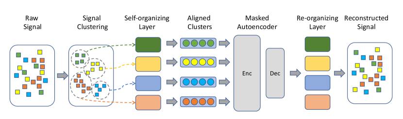
Figure 2: The overview framework of URLOST. The high-dimensional input signal undergoes clustering and self-organization before unsupervised learning using a masked autoencoder for signal reconstruction.

2.2 Density Adjusted Spectral clustering

Representation learning for high-dimensional signals without explicit topology is challenging. We propose to define a metric to measure inter-dimensional relationships. This metric effectively approximates a topology for the signal. Similar to [53], where they use the absolute correlation values as the metric for pixels, we employ discrete mutual information (refer to Appendix A.1) as the metric. Let affinity matrix $A_{ij}$ denote the mutual information between dimension $i$ and $j$, which approximates the manifold $\mathcal{M}$ that the signal lives on. We can define the discretized Laplacian operator based on $A$ and use the eigenvector of the Laplacian operator to perform spectral clustering, which segments the manifold. The detailed definition and the algorithm are left in Appendix A.1. Finding the eigenvector of the Laplacian operator is a discretized approximation of the following optimization problem in function space:

$$\min_{||f||_{L^{2}(\mathcal{M})}}\int_{\mathcal{M}}||p(x)^{\frac{1}{2}}\nabla f(x)||^{2}$$ (1)

where $f(x):\mathcal{M}\to[0,1]$ is the normalized signal defined on $\mathcal{M}$ and $p(x)$ is the density function. The integral is taken over standard measure on $\mathcal{M}$. Since spectral clustering heavily relies on the solution of equation 1, the definition of the density function $p(x)$ affects the quality of the resulting clusters. Standard approaches often assume that nodes are uniformly distributed on the manifold, thereby treating $p(x)$ as a constant and excluding it from the optimization process. However, this assumption does not hold in our case involving non-stationary signals. To cope with non-stationary signals, our work introduces a variable density function $p(x)$ for each signal, making it a pivotal component in building good representations for the signal. This component is referred to as Density Adjusted Spectral Clustering. Empirical evidence supporting this design is provided through visualization and ablation studies in the experimental section.

2.3 Self-organizing layer

Transforming a high-dimensional signal into a sequence of clusters using the above method is not enough because it does not capture the internal structure within individual clusters. To effectively perform unsupervised learning on these clusters, it is essential to align them in some manner. Directly solving the exact alignment problem with low-level statistics of the signal is challenging. Thus, we propose a self-organizing layer with learnable parameters. Specifically, let vector $x^{(i)}$ denote the $i$th cluster. Each cluster $x^{(i)}$ is passed through a differentiable function $g(\cdot,w^{(i)})$ with parameter $w^{(i)}$, resulting in a sequence $z_{0}$:

$$z_{0}=[g(x^{(1)},w^{(1)}),\cdots g(x^{(M)},w^{(M)})]$$ (2)

$z_{0}$ is comprised of projected and aligned representations for all clusters. The weights of the proposed self-organizing layer, $\{w^{(1)},\cdots w^{(M)}\}$, are jointly optimized with the subsequent neural network introduced in the next subsection.

2.4 Masked autoencoder

After the self-organizing layer, $z_{0}$ is passed to a Transformer-based masked autoencoder (MAE) with an unsupervised learning objective. Masked autoencoder (MAE) consists of an encoder and a decoder which both consist of stacked Transformer blocks introduced in [64]. The objective function is introduced in [25]: masking random image patches in an image and training an autoencoder to reconstruct them, as illustrated in Figure 1. In our case, randomly selected clusters in $z_{0}$ are masked out, and the autoencoder is trained to reconstruct these masked clusters. After training, the encoder’s output is treated as the learned representation of the input signal for downstream tasks. The masked prediction loss is computed as the mean square error (MSE) between the values of the masked clusters and their corresponding predictions.

3 Result

Since our method is inspired by the biological vision system, we first validate its ability on a synthetic biological vision dataset created from CIFAR-10. Then we evaluate the generalizability of URLOST on two high-dimensional natural datasets collected from diverse domains. Detailed information about each dataset and the corresponding experiments is presented in the following subsections. Across all tasks, URLOST consistently outperforms other strong unsupervised representation learning methods.

3.1 Synthetic biological vision dataset

As discussed in the introduction, the biological visual signal serves as an ideal dataset to validate the capability of URLOST. In contrast to digital images captured by a fixed array of sensors, the biological visual signal is acquired through irregularly positioned ganglion cells, inherently lacking explicit topology and stationarity. However, it is hard to collect real-world biological vision signals with high precision. Therefore, we employ a retinal sampling technique to modify the classic CIFAR-10 dataset and simulate imaging from the biological vision signal. The synthetic dataset is referred to as Foveated CIFAR-10. To make a comprehensive comparison, we also conduct experiments on the original CIFAR-10, and a Permuted CIFAR-10 dataset obtained by randomly permuting the image.

Permuted CIFAR-10. To remove the grid topology inherent in digital imaging, we simply permute all the pixels within the image, which effectively discards any information related to the grid structure of the original digital image. We applied such permutation to each image in the CIFAR-10 dataset to generate the Permuted CIFAR-10 dataset. Nevertheless, permuting pixels only removes an image’s topology, leaving its stationarity intact. To obtain the synthetic biological vision that has neither topology nor stationarity, we introduce the Foveated CIFAR-10.

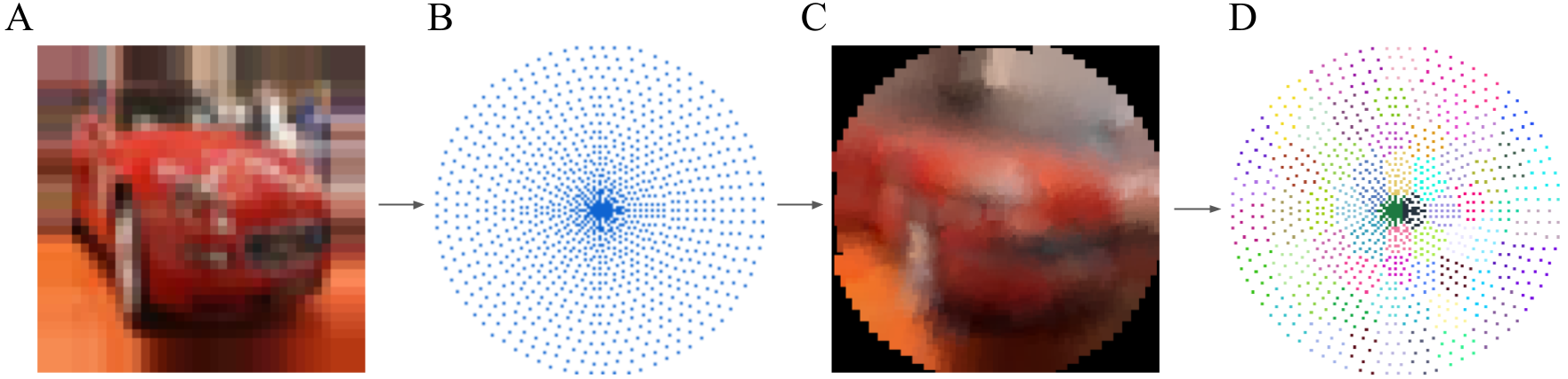
Figure 3: Retina sampling (A) An image in CIFAR-10 dataset. (B) Retina sampling lattice. Each blue dot represents the center of a Gaussian kernel, which mimics a retinal ganglion cell. (C) Visualization of the car image’s signal sampled using the retina lattice. Each kernel’s sampled RGB value is displayed at its respective lattice location for visualization purposes. (D) density-adjusted spectral clustering results are shown. Each unique color represents a cluster, with each kernel colored according to its assigned cluster.

Foveated CIFAR-10. Much like photosensors installed in a camera, retina ganglion cells within the primate biological visual system sample from visual stimuli and project images. However, unlike photosensors that have uniform receptive fields and adhere to a consistent sampling pattern, retinal ganglion cells at different locations of the retina vary in their receptive field size: smaller in the center (fovea) but larger in the peripheral of the retina. This distinctive retina sampling pattern results in foveated imaging [63]. It gives primates the ability to have both a high-resolution vision and a broad overall receptive field while consequently making visual signals sampled by the retina lack stationarity. The evidence is that responses of two ganglion cells separated by the same displacement are highly correlated in the retina but less correlated in the peripheral. To mimic the foveated imaging with CIFAR-10, we adopt the retina sampling mechanism from [8]. Specifically, each retina ganglion cell is simplified and modeled using a Gaussian kernel. The response of each cell is determined by the dot product between pixel values and the Gaussian kernel. Figure 3 illustrates the sampling kernel locations. Applying this sampling grid and permuting the resulting pixels produces the foveated CIFAR-10. In the natural retina, retinal ganglion cell density decreases linearly with eccentricity, which makes fovea much denser than the peripheral, compared to the simulated lattice in Figure 3. However, considering the low resolution of the CIFAR-10 dataset, we reduce the simulated fovea’s density to prevent redundant sampling.

Experiments. We compare URLOST on both of the synthetic vision datasets as well as the original CIFAR-10 with popular unsupervised representation learning methods SimCLR [6] and MAE [25]. All the models conducted unsupervised learning followed by linear probing for classification accuracy. The evaluations are reported in Table 1. SimCLR excels on CIFAR-10 but struggles badly with both synthetic datasets due to its inability to handle data without stationarity and topology. MAE gets close to SimCLR on CIFAR-10 with a $4\times 4$ patch size. However, the patch size no longer makes sense when data has no topology. So we additionally tested MAE masking pixels instead of image patches. It maintains the same performance on Permuted CIFAR-10 as on CIFAR-10, though poorly, invariant to the removal of topology as it should be. But It still drops greatly to $48.5\%$ on the Foveated CIFAR-10 when stationarity is also removed. In contrast, only URLOST is able to maintain consistently strong performances when there is no topology or stationarity, achieving $86.4\%$ on Permuted CIFAR-10 and $85.4\%$ on Foveated CIFAR-10 when the baselines completely fail.

Table 1: Evaluation on computer vision and synthetic biological vision dataset. ViT (Patch) stands for the Vision Transformer backbone with image patches as inputs. ViT (Pixel) means pixels are treated as input units. ViT (Clusters) means clusters are treated as inputs instead of patches. The number of clusters is set to 64 for both Permuted CIFAR-10 and Foveated CIFAR-10 dataset.

Dataset	Method	Backbone	Eval Acc
CIFAR-10	MAE	ViT (Patch)	88.3 %
	MAE	ViT (Pixel)	56.7 %
	SimCLR	ResNet-18	90.7 %
Permuted CIFAR-10	URLOST MAE	ViT (Cluster)	86.4 %
(no topology)	MAE	ViT (Pixel)	56.7 %
	SimCLR	ResNet-18	47.9 %
Foveated CIFAR-10	URLOST MAE	ViT (Cluster)	85.4 %
(no topology or stationarity)	MAE	ViT (Pixel)	48.5 %
	SimCLR	ResNet-18	38.0 %

Table 2: Evaluation on V1 response decoding and TCGA pan-cancer classification tasks. “Raw” indicates preprocessed (standardized and normalized) raw signals. Best $\beta$ values are used for $\beta$-VAE. For URLOST MAE, cluster sizes are 200 (V1) and 32 (TCGA).

Method	V1 Response Decoding Acc	TCGA Classification Acc
Raw	73.9%	91.1%
$\beta$-VAE	75.1%	94.2%
MAE	64.8%	88.3%
URLOST MAE	78.2%	94.9%

3.2 V1 neural response to natural image stimulus

After accessing URLOST’s performance on synthetic biological vision data, we take a step further to challenge its generalizability with high-dimensional natural datasets. The first task is decoding neural response recording in the primary visual area (V1) of mice.

V1 neural response dataset. The dataset, published by [44], contains responses from over 10,000 V1 neurons captured via two-photon calcium imaging. These neurons responded to 2,800 unique images from ImageNet [12], with each image presented twice to assess the consistency of the neural response. In the decoding task, a prediction is considered accurate if the neural response to a given stimulus in the first presentation closely matches the response to the same stimulus in the second presentation within the representation space. This task presents greater challenges than the synthetic biological vision described in the prior section. For one, the data comes from real-world neural recordings rather than a curated dataset like CIFAR-10. For another, the geometric structure of the V1 area is substantially more intricate than that of the retina. To date, no precise mathematical model of the V1 neural response has been well established. The inherent topology and stationarity of the data still remain difficult to grasp [43; 42]. Nevertheless, evidence of Retinotopy  [18; 19] and findings from prior research [41; 7; 58] suggest that the neuron population code in V1 are tiling a low dimensional manifold. This insight led us to treat the population neuron response as high-dimensional data and explore whether URLOST can effectively learn its representation.

Experiments. Following the approach in [44] we apply standardization and normalization to the neural firing rate. The processed signals are high-dimensional vectors, and they can be directly used for the decoding task, which serves as the “raw” signal baseline in Table 2. For representation learning methods, URLOST is evaluated along with MAE and $\beta$-VAE [26]. Note that the baseline methods need to handle high-dimensional vector data without stationarity or topology, so SimCLR is no longer applicable. We use $\beta$-VAE instead. We first train the neural network with an unsupervised learning task, then use the latent state of the network as the representation for the neural responses in the decoding task. The results are presented in the table 2. Our method surpasses the original neuron response and other methods, achieving the best performance.

3.3 Gene expression data

In this subsection, we further evaluate URLOST on high-dimensional natural science data from a completely different domain, the gene expression data.

Gene expression dataset. The dataset comes from The Cancer Genome Atlas (TCGA) [62; 66], which is a project that catalogs the genetic mutations responsible for cancer using genome sequencing and bioinformatics. The project molecularly characterized over 20,000 primary cancers and matched normal samples spanning 33 cancer types. We focus on the pan-cancer classification task: diagnose and classify the type of cancer for a given patient based on his gene expression profile. The TCGA project collects the data of 11,000 patients and uses Micro-RNA (miRNA) as their gene expression profiles. Like the V1 response, no explicit topology and stationarity are known and each data point is a high-dimensional vector. Specifically, 1773 miRNA identifiers are used so that each data point is a 1773-dimensional vector. Types of cancer that each patient is diagnosed with serve as the classification labels.

Experiments. Similar to Section 3.2, URLOST is compared with the original signals, MAE, and $\beta$-VAE, which is the state-of-the-art unsupervised learning method on TCGA cancer classification [71; 72]. We also randomly partition the dataset do five-fold cross-validation and report the average performance in Table 2. Again, our method learns meaningful representation from the original signal. The learned representation benefited the classification task and achieved the best performance, demonstrating URLOST’s ability to learn meaningful representation of data from diverse domains.

4 Ablation study

Table 3: Ablation study on self-organizing layer. Linear probing accuracy with varying parameters, keeping others constant. For Locally-Permutated CIFAR-10, we use $4\times 4$ patch size. For Permutated CIFAR-10 and Foveated CIFAR-10, we set the number of clusters to 64 for the spectral clustering algorithm. We kept the hyperparameter of the backbone model the same as in table 1.

Dataset	Projection	Eval Acc
Locally-Permuted	shared	81.4 %
CIFAR-10	non-shared	87.6 %
Permuted	shared	80.7 %
CIFAR-10	non-shared	86.4 %

(a) Replacing the non-shared projections of the self-organizing layer with the shared projection layer entails a significant drop in performance.

Dataset	Cluster	Eval Acc
Foveated	SC	82.7 %
CIFAR-10	DSC	85.4 %

(b) “SC” denotes spectral clustering with uniform density clustering and “DSC” denotes density adjusted spectral clustering. For Foveated CIFAR-10 using density adjusted spectral clustering to create clusters will make the model perform better than using standard spectral clustering with uniform density.

4.1 Self-organizing Layer vs Shared Projection Layer

Conventional SSL models take a sequential input $x=[x^{(1)},\cdots x^{(M)}]$ and embed them into latent vectors with a linear transformation:

$$z_{0}=[Ex^{(1)},\cdots Ex^{(M)}]$$ (3)

which is further processed by a neural network. The sequential inputs can be a list of language tokens [14; 50], pixel values [5], image patches [15], or overlapped image patches [6; 24; 70]. $E$ can be considered as a projection layer that is shared among all elements in the input sequence. The self-organizing layer $g(\cdot,w^{(i)})$ introduced in Section 2.3 can be considered as a non-shared projection layer. We conducted an ablation study comparing the two designs to demonstrate the effectiveness of the self-organizing layers both quantitatively and qualitatively. To facilitate the ablation, we further synthesized another dataset.

Locally-permuted CIFAR-10. To directly evaluate the performance of the non-shared projection approach, we designed an experiment involving intentionally misaligned clusters. In this experiment, we divide each image into patches and locally permute all the patches. The $i$-th image patch is denoted by $x^{(i)}$, and its permuted version, permutated by the permutation matrix $E^{(i)}$, is expressed as $E^{(i)}x^{(i)}$. We refer to this manipulated dataset as the Locally-Permuted CIFAR-10. Our hypothesis posits that models using shared projections, as defined in Equation 3, will struggle to adapt to random permutations, whereas self-organizing layers equipped with non-shared projections can autonomously adapt to each patch’s permutation, resulting in robust performance. This hypothesis is evaluated quantitatively and through the visualization of learned weights $w^{(i)}$.

Permuted CIFAR-10. Meanwhile, we also run the ablation study on the Permuted CIFAR-10. Unlike locally permuted CIFAR-10, a visualization check is not viable since the permutation is done globally. However, we can still quantitatively measure the performance of the task.

Quantitative results. Table 3 confirms our hypothesis, demonstrating a significant performance decline in models employing shared projections when exposed to permuted data. In contrast, the non-shared projection model maintains stable performance.

Visual evidence. Using linear layers to parameterize the self-organizing layers, i.e. let $g(x,W^{(i)})=W^{(i)}x$, we expect that if the projection layer effectively aligns the input sequence, $E^{(i)T}W^{(i)}$ should exhibit visual similarities. That is, after applying the inverse permutation $E^{(i)T}$, the learned projection matrix $W^{(i)}$ at each location should appear consistent or similar. The proof of this statement is provided in Appendix A.4. The model trained on Locally-Permuted CIFAR10 provides visual evidence supporting this claim. In Figure 4, the weights show similar patterns after reversing the permutations.

Figure 4: Learnt weights of a self-organizing layer. (A) Image is cropped into patches, where each patch $x^{(i)}$ first undergoes a different permutation $E^{(i)}$, then the inverse permutation $E^{(i)T}$. (B) The learned weight of the linear self-organizing layer. The $12$th column of $W^{(i)}$ at all positions $i$ are reshaped into patches and visualized. When $W^{(i)}$ undergoes the inverse permutation $E^{(i)T}$, they show similar patterns. (C) Visualization of the $37$th column of $W^{(i)}$. Similar to (B).

4.2 Density adjusted clustering vs Uniform Density Clustering

As explained in Section 2.2, the shape and size of each cluster depend on how the density function is defined. Let $q(i)$ represent the eccentricity, the distance from $i$th kernel to the center of the sampling lattice, and let $n(i)=\sum_{j}A_{ji}$ where $A$ is the affinity matrix, then the density is defined as:

$$p(i)=q(i)^{-\alpha}n(i)^{\beta}.$$ (4)

By setting $\alpha$ and $\beta$ nonzero, the density function is eccentricity-dependent. Setting both $\alpha$ and $\beta$ to zero will make $n(i)$ constant which recovers the uniform density spectral clustering. We vary the parameters $\alpha$ and $\beta$ to generate different sets of clusters for the foveated CIFAR-10 dataset and run URLOST using each of these sets of clusters. Results in Table 4 validate that the model performs better with density adjusted clustering. The intuitive explanation is that by adjusting the values of $\alpha$ and $\beta$, we can make each cluster carry similar amounts of information (refer to Appendix A.3.). A balanced distribution of information across clusters enhances the model’s ability to learn meaningful representations. Without this balance, masking a low-information cluster makes the prediction task trivial, while masking a high-information cluster will make the prediction task too difficult. In either scenario, the model’s ability to learn effective representations is compromised.

5 Additional related works

Several interconnected pursuits are linked to this work, and we will briefly address them here:

Topology in biological visual signal. 2-D topology of natural images is strong prior that requires many bits to encode [13; 2]. Such 2-D topology is encoded in the natural image statistic [55; 28], which can be recovered [53]. Optic and neural circuits in the retina result in a more irregular 2-D topology than the natural image, which can still be simulated [52; 46; 47; 45; 61; 30]. This information is further processed by the primary visual cortex. Evidence of retinotopy suggests the low-dimensional geometry of visual input from retina is encoded by the neuron in primary visual cortex [40; 20; 27; 19; 65; 48]. These evidences suggest we can recover the topology using signal from retinal ganglion cell and V1 neurons.

Evidence of self-organizing mechanism in the brain. In computational neuroscience, many works use the self-organizing maps (SOM) as a computational model for V1 functional organization: [16; 60; 1; 17; 39; 31]. In other words, this idea of self-organizing is likely a principle governing how the brain performs computations. Even though V1 functional organizations are present at birth, numerous studies also indicate that the brain’s self-organizing mechanisms continue after full development [22; 54; 29].

Learning with signal on non-euclidean geometry. In recent years, researchers from the machine learning community have made efforts to consider geometries and special structures beyond classic images, text, and feature vectors. [33] treats an image as a set of points but depends on the 2D coordinates. The geometric deep learning community tries to generalize convolution neural networks beyond the Euclidean domain [3; 37; 11; 21]. Recent research also explores adapting the Transformer to domains beyond Euclidean spaces [10; 9]. However, none of them has tried to tackle the issue when the data has no explicit topology or stationarity, which is the focus of URLOST.

Self-supervised learning. Self-supervised learning (SSL) has made substantial progress in recent years. Different SSL method is designed for each modality, for example: predicting the masked/next token in NLP[14; 50; 4], solving pre-text tasks, predicting masked patches, or building contrastive image pairs in computer vision [36; 25; 68; 6; 24; 70]. These SSL methods have demonstrated descent scalability with a vast amount of unlabeled data and have shown their power by achieving performance on par with or even surpassing supervised methods. They have also exhibited huge potential in cross-modal learning, such as the CLIP by [51]. However, we argue that these SSL methods are all built upon specific modalities with explicit topology and stationarity which URLOST goes beyond.

6 Discussion

The success of most current state-of-the-art self-supervised representation learning methods relies on the assumption that the data has known stationarity and domain topology, such as the grid-like RGB images and time sequences. However, biological vision systems have evolved to deal with signals with less regularity. In this work, we explore unsupervised representation learning under a more general assumption, where the stationarity and topology of the data are unknown to the machine learning model and its designers. We argue that this is a general and realistic assumption for high-dimensional data in modalities of natural science. We propose a novel unsupervised representation learning method that works under this assumption and demonstrates our method’s effectiveness and generality on a synthetic biological vision dataset and two datasets from natural science that have diverse modalities. We also perform a step-by-step ablation study to show the effectiveness of the novel components in our model.

During experiments, we found that density adjusted spectral clustering is crucial for the quality of representation learning. How to adjust the density and obtain a balanced clustering for any given data or even learning the clusters end-to-end with the representation via back-propagation is worth future investigation. Moreover, our current self-organizing layer is still simple though it shows effective performance. Extending it to a more sophisticated design and potentially incorporating it with various neural network architectures is also worth future exploration.

In summary, our method offers a handy and general unsupervised learning tool when dealing with high-dimensional data of arbitrary modality with unknown stationarity and topology, particularly common in the field of natural sciences, where many present strong unsupervised learning baselines cannot directly adapt. We hope it can provide inspiration for work in related fields.

Appendix A Appendix

A.1 Spectral clustering algorithm

Given a high dimensional dataset $S\in\mathbb{R}^{n\times m}$, Let $S_{i}$ be $i$th column of $S$, which represents the $i$th dimension of the signal. We create probability mass functions $P(S_{i})$ and $P(S_{j})$ and the joint distribution $P(S_{i},S_{j})$ for $S_{i}$ and $S_{j}$ using histogram. Let the number of bins be $K$. Then we measure the mutual information between $P(S_{i})$ and $P(S_{j})$ as:

$$I(S_{i};S_{j})=\sum_{l=1}^{K}\sum_{k=1}^{K}P(S_{i},S_{j})[l,k]\log_{2}\left(\frac{P(S_{i},S_{j})[l,k]}{P(S_{i})[l]P(S_{j})[k])}\right)$$

Let $A_{ij}=I(X_{i};X_{j})$ be the affinity matrix, $p(i)$ be the density function defined in 4. We follow the steps from [38] to perform spectral clustering with a modification to adjust the density:

1. Define $D$ to be the diagonal matrix whose ($i$,$i$)-element is the sum of $A$’s $i$-th row, $P$ be the identity matrix where $P_{ii}=p(i)$. Construct the matrix $L=P^{\frac{1}{2}}D^{-\frac{1}{2}}AD^{-\frac{1}{2}}P^{\frac{1}{2}}.$

2. Find $x_{1},x_{2},\cdots,x_{k}$, the $k$ largest eigenvectors of $L$, and form the matrix $X=[x_{1},x_{2},\cdots,x_{k}]\in\mathbb{R}^{n\times k}$ by stacking the eigenvectors in columns.

3. Form the matrix Y from X by renormalizing each of $X$’s rows to have unit norms. (i.e. $Y_{ij}=X_{ij}/(\sum_{i}X_{ij}^{2})^{\frac{1}{2}}$)

4. Treating each row of $Y$ as a point in $\mathbb{R}^{k}$, cluster them into $k$ clusters via K-means or other algorithms.

Some other interpretation of spectral embedding allows one to design a specific clustering algorithm in step 4. For example, [56] interprets the eigenvector problem in 1 as a relaxed continuous version of K-way normalized cuts problem, where they only allow $X$ to be binary, i.e. $X\in\{0,1\}^{N\times K}$. This is an NP-hard problem. Allowing $X$ to take on real value relaxed this problem but created a degeneracy solution. Given a solution $X^{*}$ and $Z=D^{-\frac{1}{2}}X^{*}$, for any orthonormal matrix $R$, $RZ$ is another solution to the optimization problem 1. Thus, [56] designed an algorithm to find the optimal orthonormal matrix $R$ that converts $X^{*}$ to discrete value in $\{0,1\}^{N\times K}$. From our experiment, [56] is more consistent than K-means and other clustering algorithms, so we stick to using it for our model.

A.2 Data synthesize process

We followed the retina sampling approach described in [8] to achieve foveated imaging. Specifically, each retina ganglion cell is represented using a Gaussian kernel. The kernel is parameterized by its center, denoted as $\vec{x}_{i}$, and its scalar variance, $\sigma_{i}^{\prime 2}$, i.e. $\mathcal{N}(\vec{x}_{i},\sigma_{i}^{\prime 2}\mathbf{I})$, which is illustrated in Figure 5.A. The response of each cell, denoted as $G[i]$, is computed by the dot product between the pixel value and the corresponding discrete Gaussian kernel. This can be formulated as:

$$G[i]=\sum_{n}^{N}\sum_{m}^{W}K(\vec{x}_{i},\sigma_{i}^{\prime})[n,m]I[n,m]$$

where $N$ and $W$ are dimensions of the image, and $I$ represents the image pixels.

For foveated CIFAR-10, since the image is very low resolution, we first upsample it 3 times from $32\times 32$ to $96\times 96$, then use in total of 1038 Gaussian kernels to sample from the upsampled image. The location of each kernel is illustrated in Figure 5.B. The radius of the kernel scales proportionally to the eccentricity. Here, we use the distance from the kernel to the center to represent eccentricity. The relationship between the radius of the kernel and eccentricity is shown in Figure 5.C. As mentioned in the main paper, in the natural retina, retinal ganglion cell density decreases linearly with eccentricity, which makes the fovea much denser than the peripheral, unlike the simulated lattice we created. The size of the kernel should scale linearly with respect to eccentricity as well. However, for the low-resolution CIFAR-10 dataset, we reduce the simulated fovea’s density to prevent redundant sampling. In this case, we pick the exponential scale for the relationship between the size of the kernel and eccentricity so the kernel visually covers the whole visual field. We also implemented a convolution version of the Gaussian sampling kernel to speed up data loading.

Figure 5: Foveated retinal sampling (A) Illustration of a Guassian kernel shown in [8]. Diagram of single kernel filter parameterized by a mean $\mu^{\prime}$ and variance $\sigma^{\prime}$. (B) the location of each Gaussian kernel is summarized as a point with 2D coordinate $\mu^{\prime}$. In total, the locations of 1038 Gaussian kernels are plotted. (C) The relationship between eccentricity (distance of the kernel to the center) and radius of the kernel is shown.

Table 4: Evaluation on foveated CIFAR-10 with varying hyperparameter for density function. For each set of values of $\alpha$ and $\beta$, we perform density adjusted spectral clustering and run URLOST with the corresponding cluster. The evaluation of each trial is provided in the table.

	beta = 0	beta = 2
alpha = 0	82.74 %	84.24 %
alpha = 0.5	84.52 %	85.43 %
alpha = 1.0	83.83 %	81.62 %

A.3 Density adjusted spectral clustering on foveated CIFAR10 dataset

We provide further intuition and visualization on why density adjusted spectral clustering allows the model to learn a better representation on the foveated CIFAR-10 dataset.

As shown in Figure 5, the kernel at the center is much smaller in size than the kernel in the peripheral. This makes the kernel at the center more accurate but smaller, which means it summarizes less information. Spectral clustering with constant density will make each cluster have a similar number of elements in them. Since the kernel in the center is smaller, the cluster in the center will be visually smaller, than the cluster in the peripheral. The effect is shown in Figure 6. Moreover, since we’re upsampling an already low-resolution image (CIFAR-10 image), even though the kernel at the center is more accurate, we’re not getting more information. There, to make sure each cluster has similar information, the clusters in the center need to have more elements than the clusters in the peripheral. In order to make the clusters at the center have more elements, we need to weight the clusters in the center more with the density function. Since the sampling kernels at the center have small eccentricity and are more correlated to their neighbor, increasing $\alpha$ and $\beta$ will make sampling kernels at the center have higher density, which makes the cluster at the center larger. This is why URLOST with density adjusted spectral clustering performs better than URLOST with constant density spectral clustering, which is shown in Table 4. Meanwhile, setting $\alpha$ and $\beta$ too large will also hurt the model’s performance because it creates clusters that are too unbalanced.

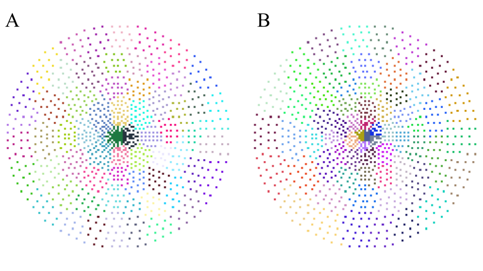
Figure 6: Effect of density adjusted clustering. Eccentricity-based sampling lattice. The center of the sampling lattice has more pixels which means higher resolution compared to the peripheral. (A) Result of density adjusted spectral clustering ($\alpha=0.5,\beta=2$). Clusters in the center have more elements than clusters in the peripheral. But clusters look more visually similar in size than B. (B) Result of uniform density spectral clustering ($\alpha=0,\beta=0$). Each cluster has a similar number of elements in them but the clusters in the center are much smaller than the clusters in the periphery.

A.4 self-organizing layer learns inverse permutation

For locally-permuted CIFAR-10, we divide each image into patches and locally permute all the patches. The $i$-th image patch is denoted by $x^{(i)}$, and its permuted version, permuted by the permutation matrix $E^{(i)}$, is expressed as $E^{(i)}x^{(i)}$. We use linear layers to parameterize the self-organizing layers. Let $g(x,W^{(i)})=W^{(i)}x$ denotes the $i$th element of the self-organizing layer. We’re providing the proof for the statement related to the visual evidence shown in Section 4.1

Statement: If the self-organizing layer effectively aligns the input sequence, then $E^{(i)T}w^{(i)}$ should exhibit visual similarities.

Proof: we first need to formally define what it means for the self-organizing layer to effectively align the input sequence. Let ${\bf e}_{k}$ denote the $k$th natural basis (one-hot vector at position $k$), which represents the pixel basis at location $k$. Permutation matrix $E^{(i)}$ will send $k$th pixel to some location accordingly. Mathematically, if the projection layer effectively aligns the input sequence, it means $g(E^{(j)}e_{k},W^{(j)})=g(E^{(i)}e_{k},W^{(i)})$ for all $i,j,k$. We can further expand this property to get the following two equations:

$$g(E^{(i)}e_{k},W^{(i)}) =W^{(i)}E^{(i)}e_{k}$$

$$g(E^{(j)}e_{k},W^{(j)}) =W^{(j)}E^{(j)}e_{k}$$

for all $i,j,k$. Since the above equation holds for all $e_{k}$, by linearity and the property of permutation matrix, we have:

$$W^{(i)}E^{(i)} =W^{(j)}E^{(j)}$$

$$E^{(i)T}W^{(i)} =E^{(j)T}W^{(j)}$$

This implies $E^{(i)T}w^{(i)}$ should exhibit visual similarities for all $i$.

A.5 Visualizing the weight of self-organizing

As explained in the previous section (Appendix A.4) and visualized in Figure 7, we can visualize the weights of the learned self-organizing layer when trained on the locally-permuted CIFAR-10 dataset. If we apply the corresponding inverse permutation $E^{(i)T}$ to its learned filter $W^{(i)}$ at position $i$, the pattern should show similarity across all position $i$. This is because the model is trying to align all the input clusters. We have shown this is the case when the model converges to a good representation. On the other hand, what if we visualize the weight $E^{(i)T}W^{(i)}$ as training goes on? If the model learns to align the clusters as it is trained for the mask prediction task, $E^{(i)T}W^{(i)}$ should become more and more consistent as training goes on. We show this visualization in Figure 7, which confirms our hypothesis. As training goes on, the pattern $E^{(i)T}W^{(i)}$ becomes more and more visually similar, which implies the model learns to gradually learn to align the input clusters.

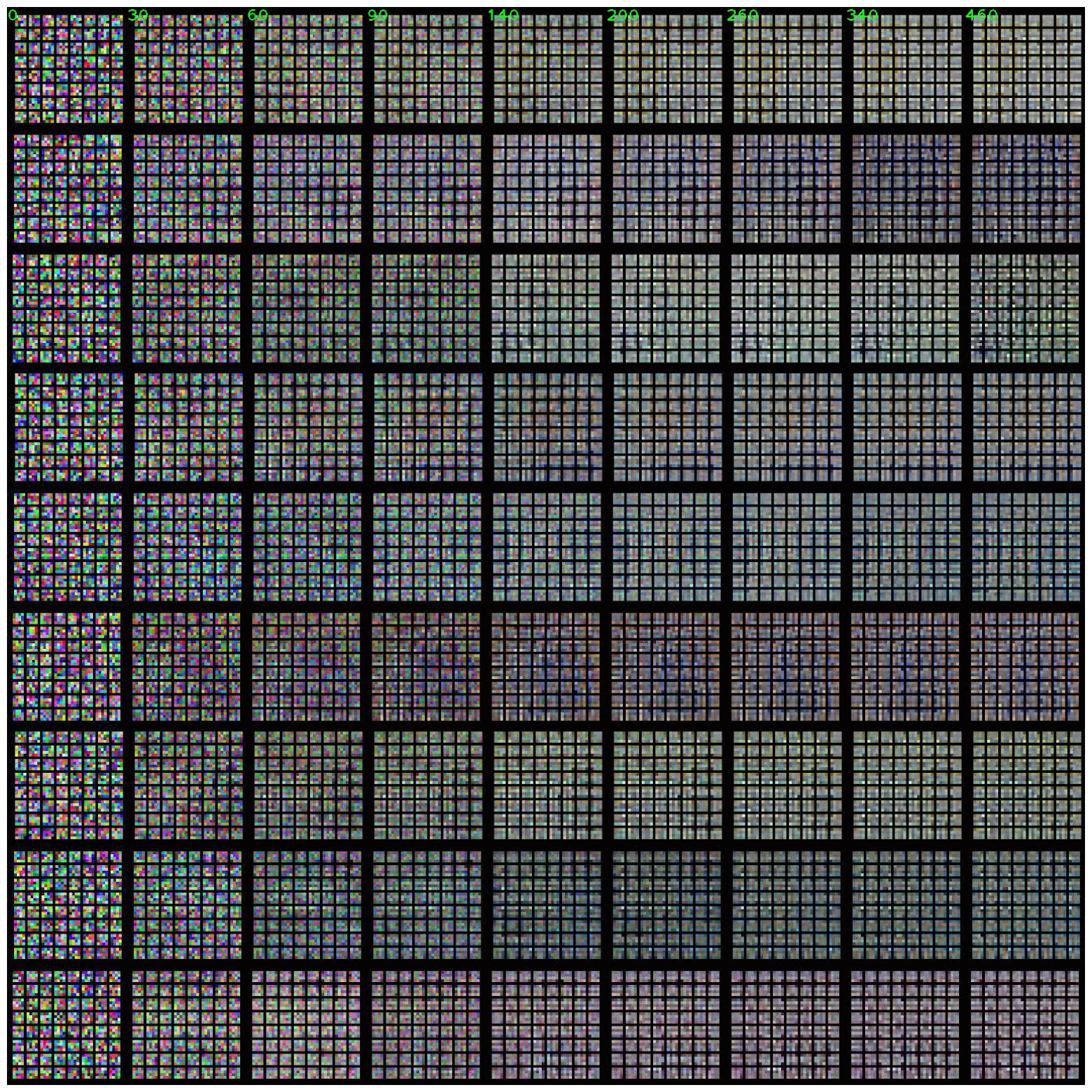
Figure 7: Visualize the weight of the self-organizing layer after applying inverse permutation. A snapshot of $E^{(i)T}W^{(i)}$ is shown at different training epoch. The number of epochs is shown on the top row. Each figure shows one column of the weight of the self-organizing layer, at different positions, i.e. $W_{:,k}^{(1)}$, where $k$ is the column number and $i$ is the position index. In total, $9$ columns are shown.

References

- Barrow et al. [1996] Harry G Barrow, Alistair J Bray, and Julian ML Budd. A self-organizing model of “color blob” formation. Neural Computation, 8(7):1427–1448, 1996.
- Bengio et al. [2007] Yoshua Bengio, Yann LeCun, et al. Scaling learning algorithms towards ai. Large-scale kernel machines, 34(5):1–41, 2007.
- Bronstein et al. [2017] Michael M Bronstein, Joan Bruna, Yann LeCun, Arthur Szlam, and Pierre Vandergheynst. Geometric deep learning: going beyond euclidean data. IEEE Signal Processing Magazine, 34(4):18–42, 2017.
- Brown et al. [2020] Tom Brown, Benjamin Mann, Nick Ryder, Melanie Subbiah, Jared D Kaplan, Prafulla Dhariwal, Arvind Neelakantan, Pranav Shyam, Girish Sastry, Amanda Askell, et al. Language models are few-shot learners. Advances in neural information processing systems, 33:1877–1901, 2020.
- Chen et al. [2020a] Mark Chen, Alec Radford, Rewon Child, Jeffrey Wu, Heewoo Jun, David Luan, and Ilya Sutskever. Generative pretraining from pixels. In International conference on machine learning, pp. 1691–1703. PMLR, 2020a.
- Chen et al. [2020b] Ting Chen, Simon Kornblith, Mohammad Norouzi, and Geoffrey Hinton. A simple framework for contrastive learning of visual representations. In International conference on machine learning, pp. 1597–1607. PMLR, 2020b.
- Chen et al. [2018] Yubei Chen, Dylan Paiton, and Bruno Olshausen. The sparse manifold transform. Advances in neural information processing systems, 31, 2018.
- Cheung et al. [2016] Brian Cheung, Eric Weiss, and Bruno A. Olshausen. Emergence of foveal image sampling from learning to attend in visual scenes. In The Fifth International Conference on Learning Representations, 2016.
- Cho et al. [2022] Sungmin Cho, Raehyuk Jung, and Junseok Kwon. Spherical transformer. arXiv preprint arXiv:2202.04942, 2022.
- Dahan et al. [2022] Simon Dahan, Logan ZJ Williams, Abdulah Fawaz, Daniel Rueckert, and Emma C Robinson. Surface analysis with vision transformers. arXiv preprint arXiv:2205.15836, 2022.
- Defferrard et al. [2016] Michaël Defferrard, Xavier Bresson, and Pierre Vandergheynst. Convolutional neural networks on graphs with fast localized spectral filtering. Advances in neural information processing systems, 29, 2016.
- Deng et al. [2009] Jia Deng, Wei Dong, Richard Socher, Li-Jia Li, Kai Li, and Li Fei-Fei. Imagenet: A large-scale hierarchical image database. In 2009 IEEE conference on computer vision and pattern recognition, pp. 248–255. Ieee, 2009.
- Denker & leCun [1992] J.S. Denker and Y. leCun. Natural versus ”universal” probability, complexity, and entropy. In Workshop on Physics and Computation, pp. 122–127, 1992. doi: 10.1109/PHYCMP.1992.615508.
- Devlin et al. [2019] Jacob Devlin, Ming-Wei Chang, Kenton Lee, and Kristina Toutanova. Bert: Pre-training of deep bidirectional transformers for language understanding. In North American Chapter of the Association for Computational Linguistics, 2019.
- Dosovitskiy et al. [2021] Alexey Dosovitskiy, Lucas Beyer, Alexander Kolesnikov, Dirk Weissenborn, Xiaohua Zhai, Thomas Unterthiner, Mostafa Dehghani, Matthias Minderer, Georg Heigold, Sylvain Gelly, Jakob Uszkoreit, and Neil Houlsby. An image is worth 16x16 words: Transformers for image recognition at scale. In International Conference on Learning Representations, 2021.
- Durbin & Mitchison [1990a] Richard Durbin and Graeme Mitchison. A dimension reduction framework for understanding cortical maps. Nature, 343(6259):644–647, 1990a. doi: 10.1038/343644a0.
- Durbin & Mitchison [1990b] Richard Durbin and Graeme Mitchison. A dimension reduction framework for understanding cortical maps. Nature, 343(6259):644–647, 1990b.
- Ellis et al. [2021] Cameron T Ellis, Tristan S Yates, Lena J Skalaban, Vikranth R Bejjanki, Michael J Arcaro, and Nicholas B Turk-Browne. Retinotopic organization of visual cortex in human infants. Neuron, 109(16):2616–2626, 2021.
- Engel et al. [1997] Stephen A Engel, Gary H Glover, and Brian A Wandell. Retinotopic organization in human visual cortex and the spatial precision of functional mri. Cerebral cortex (New York, NY: 1991), 7(2):181–192, 1997.
- Felleman & Van Essen [1991] Daniel J Felleman and David C Van Essen. Distributed hierarchical processing in the primate cerebral cortex. Cerebral cortex (New York, NY: 1991), 1(1):1–47, 1991.
- Fey et al. [2018] Matthias Fey, Jan Eric Lenssen, Frank Weichert, and Heinrich Müller. Splinecnn: Fast geometric deep learning with continuous b-spline kernels. In Proceedings of the IEEE/CVF Conference on Computer Vision and Pattern Recognition, pp. 869–877, 2018.
- Gilbert & Li [2012] Charles D Gilbert and Wu Li. Adult visual cortical plasticity. Neuron, 75(2):250–264, 2012.
- Haghighi et al. [2022] Marzieh Haghighi, Juan C. Caicedo, Beth A. Cimini, Anne E. Carpenter, and Shantanu Singh. High-dimensional gene expression and morphology profiles of cells across 28,000 genetic and chemical perturbations. Nature Methods, 19(12):1550–1557, 2022. doi: 10.1038/s41592-022-01667-0.
- He et al. [2020] Kaiming He, Haoqi Fan, Yuxin Wu, Saining Xie, and Ross Girshick. Momentum contrast for unsupervised visual representation learning. In Proceedings of the IEEE/CVF conference on computer vision and pattern recognition, pp. 9729–9738, 2020.
- He et al. [2022] Kaiming He, Xinlei Chen, Saining Xie, Yanghao Li, Piotr Dollár, and Ross Girshick. Masked autoencoders are scalable vision learners. In Proceedings of the IEEE/CVF Conference on Computer Vision and Pattern Recognition, pp. 16000–16009, 2022.
- Higgins et al. [2016] Irina Higgins, Loic Matthey, Arka Pal, Christopher Burgess, Xavier Glorot, Matthew Botvinick, Shakir Mohamed, and Alexander Lerchner. beta-vae: Learning basic visual concepts with a constrained variational framework. In International conference on learning representations, 2016.
- Hubel & Wiesel [1962] David H Hubel and Torsten N Wiesel. Receptive fields, binocular interaction and functional architecture in the cat’s visual cortex. The Journal of physiology, 160(1):106, 1962.
- Hyvärinen et al. [2009] Aapo Hyvärinen, Jarmo Hurri, and Patrick O Hoyer. Natural image statistics: A probabilistic approach to early computational vision., volume 39. Springer Science & Business Media, 2009.
- Jamal & Dilks [2020] Yaseen A Jamal and Daniel D Dilks. Rapid topographic reorganization in adult human primary visual cortex (v1) during noninvasive and reversible deprivation. Proceedings of the National Academy of Sciences, 117(20):11059–11067, 2020.
- Jonnalagadda et al. [2021] Aditya Jonnalagadda, William Yang Wang, BS Manjunath, and Miguel P Eckstein. Foveater: Foveated transformer for image classification. arXiv preprint arXiv:2105.14173, 2021.
- Kohonen [1982] Teuvo Kohonen. Self-organized formation of topologically correct feature maps. Biological cybernetics, 43(1):59–69, 1982.
- Krizhevsky et al. [2014] Alex Krizhevsky, Vinod Nair, and Geoffrey Hinton. The cifar-10 dataset. online: http://www. cs. toronto. edu/kriz/cifar. html, 55(5), 2014.
- Ma et al. [2023] Xu Ma, Yuqian Zhou, Huan Wang, Can Qin, Bin Sun, Chang Liu, and Yun Fu. Image as set of points. In The Eleventh International Conference on Learning Representations, 2023.
- Mehrizi et al. [2023] Rahil Mehrizi, Arash Mehrjou, Maryana Alegro, Yi Zhao, Benedetta Carbone, Carl Fishwick, Johanna Vappiani, Jing Bi, Siobhan Sanford, Hakan Keles, et al. Multi-omics prediction from high-content cellular imaging with deep learning. arXiv preprint arXiv:2306.09391, 2023.
- Meyer [1983] Ronald L Meyer. Tetrodotoxin inhibits the formation of refined retinotopography in goldfish. Developmental Brain Research, 6(3):293–298, 1983.
- Misra & Maaten [2020] Ishan Misra and Laurens van der Maaten. Self-supervised learning of pretext-invariant representations. In Proceedings of the IEEE/CVF conference on computer vision and pattern recognition, pp. 6707–6717, 2020.
- Monti et al. [2016] Federico Monti, Davide Boscaini, Jonathan Masci, Emanuele Rodola, Jan Svoboda, and Michael M Bronstein. Geometric deep learning on graphs and manifolds using mixture model cnns. In Proceedings of the IEEE/CVF conference on computer vision and pattern recognition, 2016.
- Ng et al. [2001] Andrew Ng, Michael Jordan, and Yair Weiss. On spectral clustering: Analysis and an algorithm. Advances in neural information processing systems, 14, 2001.
- Obermayer et al. [1990] Klaus Obermayer, Helge Ritter, and Klaus Schulten. A principle for the formation of the spatial structure of cortical feature maps. Proceedings of the National Academy of Sciences, 87(21):8345–8349, 1990.
- Ogmen & Herzog [2010] Haluk Ogmen and Michael H Herzog. The geometry of visual perception: Retinotopic and nonretinotopic representations in the human visual system. Proceedings of the IEEE, 98(3):479–492, 2010.
- Olshausen & Field [1996] Bruno A Olshausen and David J Field. Emergence of simple-cell receptive field properties by learning a sparse code for natural images. Nature, 381(6583):607–609, 1996.
- Olshausen & Field [2005] Bruno A Olshausen and David J Field. How close are we to understanding v1? Neural computation, 17(8):1665–1699, 2005.
- Olshausen & Field [2006] Bruno A Olshausen and David J Field. What is the other 85 percent of v1 doing. L. van Hemmen, & T. Sejnowski (Eds.), 23:182–211, 2006.
- Pachitariu et al. [2016] Marius Pachitariu, Carsen Stringer, Sylvia Schröder, Mario Dipoppa, L Federico Rossi, Matteo Carandini, and Kenneth D Harris. Suite2p: beyond 10,000 neurons with standard two-photon microscopy. BioRxiv, pp. 061507, 2016.
- Peli et al. [1991] Eli Peli, Jian Yang, and Robert B Goldstein. Image invariance with changes in size: The role of peripheral contrast thresholds. JOSA A, 8(11):1762–1774, 1991.
- Perry & Geisler [2002] Jeffrey S Perry and Wilson S Geisler. Gaze-contingent real-time simulation of arbitrary visual fields. In Human vision and electronic imaging VII, volume 4662, pp. 57–69. SPIE, 2002.
- Pointer & Hess [1989] JS Pointer and RF Hess. The contrast sensitivity gradient across the human visual field: With emphasis on the low spatial frequency range. Vision research, 29(9):1133–1151, 1989.
- Polimeni et al. [2010] Jonathan R Polimeni, Bruce Fischl, Douglas N Greve, and Lawrence L Wald. Laminar analysis of 7 t bold using an imposed spatial activation pattern in human v1. Neuroimage, 52(4):1334–1346, 2010.
- Probst & Reymond [2020] Daniel Probst and Jean-Louis Reymond. Visualization of very large high-dimensional data sets as minimum spanning trees. Journal of Cheminformatics, 12(1):12, 2020. doi: 10.1186/s13321-020-0416-x.
- Radford et al. [2018] Alec Radford, Karthik Narasimhan, Tim Salimans, Ilya Sutskever, et al. Improving language understanding by generative pre-training. 2018.
- Radford et al. [2021] Alec Radford, Jong Wook Kim, Chris Hallacy, Aditya Ramesh, Gabriel Goh, Sandhini Agarwal, Girish Sastry, Amanda Askell, Pamela Mishkin, Jack Clark, et al. Learning transferable visual models from natural language supervision. In International conference on machine learning, pp. 8748–8763. PMLR, 2021.
- Roorda & Williams [1999] Austin Roorda and David R Williams. The arrangement of the three cone classes in the living human eye. Nature, 397(6719):520–522, 1999.
- Roux et al. [2007] Nicolas Roux, Yoshua Bengio, Pascal Lamblin, Marc Joliveau, and Balázs Kégl. Learning the 2-d topology of images. In J. Platt, D. Koller, Y. Singer, and S. Roweis (eds.), Advances in Neural Information Processing Systems, volume 20. Curran Associates, Inc., 2007.
- Sammons & Keck [2015] Rosanna P Sammons and Tara Keck. Adult plasticity and cortical reorganization after peripheral lesions. Current Opinion in Neurobiology, 35:136–141, 2015.
- Simoncelli & Olshausen [2001] Eero P Simoncelli and Bruno A Olshausen. Natural image statistics and neural representation. Annual review of neuroscience, 24(1):1193–1216, 2001.
- Stella & Shi [2003] X Yu Stella and Jianbo Shi. Multiclass spectral clustering. In Computer Vision, IEEE International Conference on, volume 2, pp. 313–313. IEEE Computer Society, 2003.
- Stringer et al. [2018] Carsen Stringer, Marius Pachitariu, Matteo Carandini, and Kenneth Harris. Recordings of 10,000 neurons in visual cortex in response to 2,800 natural images. Figshare Repos, 2018.
- Stringer et al. [2019] Carsen Stringer, Marius Pachitariu, Nicholas Steinmetz, Matteo Carandini, and Kenneth D Harris. High-dimensional geometry of population responses in visual cortex. Nature, 571(7765):361–365, July 2019.
- Stringer et al. [2021] Carsen Stringer, Michalis Michaelos, Dmitri Tsyboulski, Sarah E. Lindo, and Marius Pachitariu. High-precision coding in visual cortex. Cell, 184(10):2767–2778.e15, 2021. ISSN 0092-8674. doi: https://doi.org/10.1016/j.cell.2021.03.042.
- Swindale & Bauer [1998] Nicholas V. Swindale and Hans-Ulrich Bauer. Application of kohonen’s self-organizing feature map algorithm to cortical maps of orientation and direction preference. Proceedings: Biological Sciences, 265(1398):827–838, 1998. ISSN 09628452.
- Thibos [1998] Larry N Thibos. Acuity perimetry and the sampling theory of visual resolution. Optometry and vision science: official publication of the American Academy of Optometry, 75(6):399–406, 1998.
- Tomczak et al. [2015] Katarzyna Tomczak, Patrycja Czerwińska, and Maciej Wiznerowicz. Review the cancer genome atlas (tcga): an immeasurable source of knowledge. Contemporary Oncology/Współczesna Onkologia, 2015(1):68–77, 2015.
- Van Essen et al. [1992] David C Van Essen, Charles H Anderson, and Daniel J Felleman. Information processing in the primate visual system: an integrated systems perspective. Science, 255(5043):419–423, 1992.
- Vaswani et al. [2017] Ashish Vaswani, Noam Shazeer, Niki Parmar, Jakob Uszkoreit, Llion Jones, Aidan N Gomez, Łukasz Kaiser, and Illia Polosukhin. Attention is all you need. Advances in neural information processing systems, 30, 2017.
- Wandell et al. [2007] Brian A Wandell, Serge O Dumoulin, and Alyssa A Brewer. Visual field maps in human cortex. Neuron, 56(2):366–383, 2007.
- Weinstein et al. [2013] John N Weinstein, Eric A Collisson, Gordon B Mills, Kenna R Shaw, Brad A Ozenberger, Kyle Ellrott, Ilya Shmulevich, Chris Sander, and Joshua M Stuart. The cancer genome atlas pan-cancer analysis project. Nature genetics, 45(10):1113–1120, 2013.
- Wong [1999] Rachel OL Wong. Retinal waves and visual system development. Annual review of neuroscience, 22(1):29–47, 1999.
- Wu et al. [2018] Zhirong Wu, Yuanjun Xiong, Stella X. Yu, and Dahua Lin. Unsupervised feature learning via non-parametric instance discrimination. In Proceedings of the IEEE Conference on Computer Vision and Pattern Recognition (CVPR), June 2018.
- Xu et al. [2021] Youzheng Xu, Yixin Xu, Chun Wang, Baoguo Xia, Qingling Mu, Shaohong Luan, and Jun Fan. Mining tcga database for gene expression in ovarian serous cystadenocarcinoma microenvironment. PeerJ, 9:e11375, 2021.
- Zbontar et al. [2021] Jure Zbontar, Li Jing, Ishan Misra, Yann LeCun, and Stéphane Deny. Barlow twins: Self-supervised learning via redundancy reduction. In International Conference on Machine Learning, pp. 12310–12320. PMLR, 2021.
- Zhang et al. [2019] Xiaoyu Zhang, Jingqing Zhang, Kai Sun, Xian Yang, Chengliang Dai, and Yike Guo. Integrated multi-omics analysis using variational autoencoders: Application to pan-cancer classification. In 2019 IEEE International Conference on Bioinformatics and Biomedicine (BIBM), pp. 765–769, 2019. doi: 10.1109/BIBM47256.2019.8983228.
- Zhang et al. [2021] Xiaoyu Zhang, Yuting Xing, Kai Sun, and Yike Guo. Omiembed: A unified multi-task deep learning framework for multi-omics data. Cancers, 13(12), 2021. ISSN 2072-6694. doi: 10.3390/cancers13123047.