Diffusing on Two Levels and Optimizing for Multiple Properties: A Novel Approach to Generating Molecules with Desirable Properties

Abstract

In the past decade, Artificial Intelligence (AI) driven drug design and discovery has been a hot research topic in the AI area, where an important branch is molecule generation by generative models, from GAN-based models and VAE-based models to the latest diffusion-based models. However, most existing models pursue only the basic properties like validity and uniqueness of the generated molecules, a few go further to explicitly optimize one single important molecular property (e.g. QED or PlogP), which makes most generated molecules little usefulness in practice. In this paper, we present a novel approach to generating molecules with desirable properties, which expands the diffusion model framework with multiple innovative designs. The novelty is two-fold. On the one hand, considering that the structures of molecules are complex and diverse, and molecular properties are usually determined by some substructures (e.g. pharmacophores), we propose to perform diffusion on two structural levels: molecules and molecular fragments respectively, with which a mixed Gaussian distribution is obtained for the reverse diffusion process. And to get desirable molecular fragments, we develop a novel electronic effect based fragmentation method. On the other hand, we introduce two ways to explicitly optimize multiple molecular properties under the diffusion model framework. First, as potential drug molecules must be chemically valid, we optimize molecular validity by an energy-guidance function. Second, since potential drug molecules should be desirable in various properties, we employ a multi-objective mechanism to optimize multiple molecular properties simultaneously. Extensive experiments with two benchmark datasets QM9 and ZINC250k show that the molecules generated by our proposed method have better validity, uniqueness, novelty, Fréchet ChemNet Distance (FCD), QED, and PlogP than those generated by current SOTA models.

1 Introduction

The fundamental goal of drug design and discovery is to find candidate molecules that have the desirable chemical properties. Traditional drug design relies heavily on the expertise of pharmaceutical professionals. With a high failure rate up to 96%, this process can take decades of years and cost billions of dollars [1; 2]. With the remarkable advances in artificial intelligence (AI) techniques, the situation has been changing. In the past decade, an increasing number of AI models and algorithms have been involved in drug design and discovery, which brings in the blossoming area of AI-driven drug design and discovery. Among these efforts, a hot and promising research direction is automatic molecule generation by generative models. Especially, by efficiently exploring the vast chemical space and accurately modeling various molecules, recent deep generative models have been blazing a trail in accelerating the drug discovery process and reducing cost. Typically, these models first learn a continuous latent space by encoding the training molecules and then generate new molecules by decoding the learned latent space [3; 4; 5]. Up to now, a number of molecule generation models have been developed, which roughly fall into four types, including GAN-based models, VAE-based models, energy-based models, flow-based models, and the latest diffusion-based models.

However, most existing molecule generation models stop at pursuing high basic properties like validity and uniqueness of the generated molecules, only a few go further to explicitly optimize one single more important property such as QED or PlogP. As potential drug molecules should be desirable for all properties, so most generated molecules of current models are actually of limited usefulness. To challenge this situation, in this paper we try to generate molecules with multiple desirable properties, i.e., we generate molecules with multiple properties optimized simultaneously.

To this end, we propose a novel approach by expanding the diffusion model framework with multiple innovative designs. The novelty of our approach lies in two aspects:

On the one hand, considering that molecules are complex and diverse in structure, and molecular properties are heavily dependent on some substructures (e.g. pharmacophores) of molecules, we think that directly modeling the whole molecular space with a limited number of real molecules may be not enough. Different from the existing diffusion-based models, we perform diffusion on two structural levels: molecules and molecular fragments respectively. A mixed Gaussian distribution is obtained from the two levels’ diffused Gaussian distributions and applied to the reverse diffusion process. As we hope that the fragments are really related to molecular properties, instead of using existing molecule fragmentation scheme like BRICS [6], we develop a new fragmentation method based on electronic effect, which is a physicochemical measure of molecules or molecular fragments, related to their acidity and alkalinity.

On the other hand, we design two strategies to optimize multiple properties simultaneously. First, considering that potential drug molecules must be chemically valid, we optimize the validity of molecules by an energy-guidance function to control the denoising process. Second, as potential drug molecules should be desirable in various properties, routine strategies that combine different properties into one indicator to be optimized, do not work well. Instead, we employ a multiple-objective mechanism to optimize multiple molecular properties simultaneously so that all properties can reach a desirable state.

To demonstrate the effectiveness and advantages of the proposed method, we carry out extensive experiments with two benchmark datasets QM9 [7] and ZINC250k [8]. Seven typical existing models, covering SOTA VAE-based model [9], flow-based models  [10; 11; 12; 4], and diffusion-based models [13; 14] are used for performance comparison. Comprehensive ablation studies are also conducted to validate the effects of different model designs and parameter settings.

Our contributions are summarized as follows: 1) We propose a novel approach to generating molecules with desirable properties. To the best of our knowledge, this is the first work that optimizes multiple properties of the generated molecules simultaneously. 2) To model the molecules better, we develop a generative model that diffuses on two molecular structural levels— molecules and molecular fragments respectively. We also introduce a new molecule fragmentation method based on electronic effect. 3) We employ two ways to optimize multiple properties of generated molecules under the diffusion model framework. On the one hand, we use an energy guidance function to optimize molecular validity. On the other hand, we adopt a multiple-objective strategy to optimize other properties. 4) We conduct extensive experiments with two benchmark datasets. The results show that compared to typical existing models, the proposed method can generate molecules with better validity, uniqueness, novelty, Fréchet ChemNet Distance (FCD), QED, and PlogP.

2 Related Work

Existing deep generative models for molecule generation fall roughly into five types, including GAN-based, VAE-based, energy-based, flow-based, and recent diffusion-based models.

GAN-based models. Early works of deep molecular generation models are mostly based on GANs, where the distribution of the training set is implicitly learned by the competition learning of the generator and the discriminator. Typical GAN-based models include ORGAN [15], MolGAN [16], and GA-GAN [17]. These models can achieve high novelty due to implicit and likelihood-free features, but their validity/uniqueness is limited. Due to the inherent problems with GANs such as perfect discriminator and mode collapse, it is challenging to train GAN-based models, and difficult to generate molecules with desirable molecular properties.

VAE-based models. Up to now, a number of VAE-based molecular generation models have been developed, including GraphVAE [18], JTVAE [9], CGVAE [19], and NeVAE [20]. In these models, the data distribution is learned by the identification model (encoder) and the generation model (decoder) [21]. Although the optimization of VAE-based models is easier and more stable than GAN-based models [16], only the lower bound of log-likelihood is optimized, which thus limits the generative power of the networks.

Energy-based models. These models try to model the energy function of molecules, by assigning lower energies to data points corresponding to real molecules and higher energies to other data points. GraphEBM [22] is a representative of such models. Energy-based models are usually difficult to train due to the slow sampling process. To optimize a energy model, many estimations must be done, the inefficiency problem of energy model training will be exacerbated [23].

Flow-based models. They directly optimize the log-likelihood function to model the generative probability of samples. Typical flow-based molecular generation models are GraphAF [11], GraphDF [12] and MoFlow [4]. Most of these models fail to capture the permutation-invariance property of molecular graphs [22] and are computationally expensive.

Diffusion-based models. They stand for the cutting-edge deep generative models, which gradually perturb the training dataset through a forward diffusion process, and then sample new data from the same distribution by gradually denoising in the reverse diffusion process. With the advantages of tractable training, flexible expansion, and permutation-invariant, such models have excellent performance in molecule generation. GDSS [13] captures the joint distribution of molecular nodes and edges, only to generate mere molecular imitations close to the training distribution. DiGress [14] is more efficient than GDSS by a discrete diffusion process, but the properties of generated molecules are relatively low.

Differences between existing models and our work. First, different from existing models, we try to generate molecules with multiple desirable properties, not only basic properties like validity and uniqueness but also more important properties such as QED and PlogP. Second, different from current diffusion-based models, we perform diffusion on two structural levels — molecules and fragments respectively, and use the resulting mixed Gaussian distribution for the reverse process. Third, our work is the first that uses multiple-objective optimization to coordinate multiple properties.

3 Methodology

In this section, we first describe the framework of our work to give an overview of the proposed method. Then, we introduce our techniques in detail.

3.1 Overview

Fig. 1 shows the framework of our D2L-OMP method, which is an expanded diffusion model with multiple innovative designs. It consists of three major modules: (a) the method of molecule fragmentation based on electronic effect (FREE in short), (b) the generative model diffusing on two molecular structural levels (D2L in short), and (c) the module of optimization for multiple molecular properties (OMP in short). Each training molecule is fragmented by the FREE method, which will be introduced in Sec. 3.2. All the fragments generated by FREE form a fragment vocabulary used for model training. Take all fragments in the vocabulary and the training molecules as input, the model is trained by first diffusing on two molecular structural levels — the fragments and the molecules respectively, from which two Gaussian distributions are obtained, which are further combined to get a mixed Gaussian distribution, then denoising the mixed Gaussian distribution in the reverse diffusion process. The model will be detailed in Sec. 3.3. During model training, we try to optimize multiple molecular properties simultaneously by two strategies, which are presented in Sec. 3.4 and Sec. 3.5 respectively. On the one hand, we optimize the validity of generated molecules based on an energy guidance function, as validity is a basic property of generated molecules. On the other hand, we employ multi-objective optimization to optimize multiple molecular properties, which can make multiple properties desirable. In this paper, without loss of generality, we optimize validity, QED, and PlogP. Actually, our method can be expanded to optimize more properties.

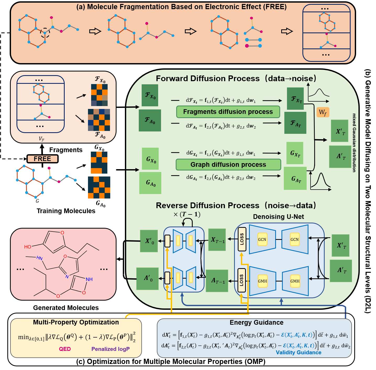
Figure 1: The framework of the D2L-OMP method.

3.2 Molecule Fragmentation Based on Electronic Effect

Generally, we hope that the fragments are closely associated with molecular properties. Actually, there are already a number of molecule fragmentation schemes in the literature, including BRICS [6]. However, our experiments show that fragments generated by those schemes are not satisfactory in our work (also see the ablation results in Sec. 4.2.2). So we propose a new fragmentation method based on electronic effect [24].

Electronic effects happen when the substituents of molecules cause the distribution change of the electron cloud density within molecules, consequently impacting the acidity or alkalinity of substituents and molecules. Substituents are qualified by the substituent constant. The Hammett equation, which describes the relationship between the substituent constant and the equilibrium constant when the reaction type is determined, is used to calculate the substituent constant $\sigma$  [25; 26; 27]: $\sigma=\frac{1}{\rho}log\dfrac{K}{K_{0}},$ where $\rho$ is the reaction constant, which is related only to the type of reaction. $K$ is the equilibrium constant when the substituent is not a hydrogen atom, and $K_{0}$ is the equilibrium constant when the substituent is a hydrogen atom. In [26], various substituents and their constants are presented in the so-called Hammett table.

Given a molecule, we fragment it as follows: 1) Split all ring substructures from their chain substructures, resulting in a set $R$={$R_{i}$} of ring substructures and a set $C$={$C_{i}$} of chain substructures, $R_{i}$ and $C_{i}$ are a ring substructure and a chain substructure respectively. 2) We directly accept all elements in $R$ as fragments. 3) For each element $C_{i}$ in $C$, first use the substituent with the highest constant in the Hammett table to search matching substructures in $C_{i}$, and accept the hits as fragments, meanwhile removing the matched substructures from $C_{i}$, and denoting the remaining as $C_{i}^{\prime}$; Then, use the substituent with the second highest constant in the Hammett table to search matching substructures in $C_{i}^{\prime}$, and save the hits as fragments. The above process goes iteratively till no more match can be found. 4) Using $\sigma_{R}$ as a threshold to filter out the fragments with constant $\left|\sigma\right|$ $<$ $\sigma_{R}$, the remaining fragments form the final fragment set. In our experiments, we set the $R=$hydrogen atom, i.e., using the $\sigma_{H}$ as the threshold value. In such a way, we can get all fragments from the training molecules, which form a fragment vocabulary $V_{\boldsymbol{\mathcal{F}}}$. In this paper, we call $V_{\boldsymbol{\mathcal{F}}}$ the FREE vocabulary, and all fragments FREE fragments.

3.3 Diffusion on Two Molecular Structural Levels

For a molecular graph $\boldsymbol{G}$ with $m$ nodes (atoms), we have $\boldsymbol{G}=(\boldsymbol{G}_{X},\boldsymbol{G}_{A})$ where $\boldsymbol{G}_{X}\in{\mathbb{R}^{m\times{dim}}}$ and $\boldsymbol{G}_{A}\in{\mathbb{R}^{m\times{m}}}$ are the node feature matrix and the weighted adjacency matrix respectively, $dim$ is the dimension of the node features. Similarly, for a FREE fragment $\boldsymbol{\mathcal{F}}$ with $n$ nodes, we have $\boldsymbol{\mathcal{F}}=(\boldsymbol{\mathcal{F}}_{X},\boldsymbol{\mathcal{F}}_{A})$ where $\boldsymbol{\mathcal{F}}_{X}\in{\mathbb{R}^{n\times{dim}}}$ and $\boldsymbol{\mathcal{F}}_{A}\in{\mathbb{R}^{n\times{n}}}$ are the node feature matrix and the weighted adjacency matrix respectively. To train the D2L-OMP model, all training molecular graphs and the corresponding FREE fragments are used, on which the diffusion is performed respectively.

By step-wisely injecting noise, the training molecular graphs and fragments are respectively and smoothly transformed into a Gaussian distribution, they are then combined into a mixed Gaussian distribution. Inspired by [13], to successfully generate samples from the data distribution, the node feature matrix and weighted adjacency matrix of each molecular graph should be diffused simultaneously. Denote the forward diffusion process on the molecular graph $\boldsymbol{G}$ as $\{\boldsymbol{G}_{t}=(\boldsymbol{G}_{X_{t}},\boldsymbol{G}_{A_{t}})\}_{t=0}^{T}$ in a fixed time horizon $t\in[0,T]$, which can be modeled as the solution to an $It$$\widehat{o}$ SDE:

$$\mathrm{d}\boldsymbol{G}_{t}=\mathbf{f}_{t}(\boldsymbol{G}_{t})\mathrm{d}t+g(t)\mathrm{d}\boldsymbol{\mathrm{w}},\boldsymbol{G}_{0}\sim p_{mol},$$ (1)

where $\boldsymbol{G}_{0}$ is a graph from the data distribution $p_{mol}$, $\mathbf{f}_{t}(\cdot)$, $g(\cdot)$ and $\boldsymbol{\mathrm{w}}$ are the linear drift coefficient, the diffusion coefficient, and the standard Wiener process, respectively. In Eq. (1), at each infinitesimal time step $\mathrm{d}t$, an infinitesimal noise $\mathrm{d}\boldsymbol{\mathrm{w}}$ is added to $\boldsymbol{G}_{X_{0}}$ and $\boldsymbol{G}_{A_{0}}$. The coefficients $\mathbf{f}_{t}(\cdot)$ and $g(\cdot)$ are related to the size of noise. To efficiently generate samples, the sample $\boldsymbol{G}_{t}$ approximately follows a prior distribution with a tractable form (e.g. a Gaussian distribution).

Similarly, the forward diffusion process on a FREE fragment $\boldsymbol{\mathcal{F}}$ can be denoted as $\{\boldsymbol{\mathcal{F}}_{t}=(\boldsymbol{\mathcal{F}}_{X_{t}},\boldsymbol{\mathcal{F}}_{A_{t}})\}_{t=0}^{T}$ in a fixed time horizon $t\in[0,T]$, which can be modeled as the solution to an $It$$\widehat{o}$ SDE: $\mathrm{d}\boldsymbol{\mathcal{F}}_{t}=\mathbf{f}_{t}(\boldsymbol{\boldsymbol{\mathcal{F}}}_{t})\mathrm{d}t+g(t)\mathrm{d}\boldsymbol{\mathrm{w}},\boldsymbol{\mathcal{F}}_{0}\sim p_{\mathcal{F}}$.

Since the sum of two independent Gaussian distributions is still a Gaussian distribution.We expand the dimension of $\boldsymbol{\mathcal{F}}_{T}$ to be consistent with the $\boldsymbol{G}_{T}$. The diffused sample $\boldsymbol{G}_{T}=(\boldsymbol{G}_{X_{T}},\boldsymbol{G}_{A_{T}})$ and $\boldsymbol{\mathcal{F}}_{T}=(\boldsymbol{\mathcal{F}}_{X_{T}},\boldsymbol{\mathcal{F}}_{A_{T}})$ are mixed into a new Gaussian distribution $\boldsymbol{G^{\prime}}_{T}=(\boldsymbol{X^{\prime}}_{T},\boldsymbol{A^{\prime}}_{T})$:

$$\boldsymbol{G^{\prime}}_{T}=\boldsymbol{G}_{T}+\mathrm{W}_{f}\boldsymbol{\mathcal{F}}_{T},$$ (2)

$$\left\{\begin{array}[]{c}\boldsymbol{X^{\prime}}_{T}=\boldsymbol{G}_{X_{T}}+\mathrm{W}_{f}\boldsymbol{\mathcal{F}}_{X_{T}},\\ \boldsymbol{A^{\prime}}_{T}=\boldsymbol{G}_{A_{T}}+\mathrm{W}_{f}\boldsymbol{\mathcal{F}}_{A_{T}},\end{array}\right.$$ (3)

where $\mathrm{W}_{f}$ is a weight (or hyperparameter) to control the influence of FREE fragments on the mixed Gaussian distribution.

3.4 Energy Guidance Function

To promote the generation of molecules of high validity, in this section, we introduce an energy guidance function as a constraint on the generation process where the noise added in the forward diffusion process is step-wisely removed during the reverse diffusion process. Because the energy function can capture dependencies between two variables [28], we use low energy to indicate that the generated molecules meet the desired properties (e.g. high validity), which in turn encourages the model to generate more low-energy molecules while discarding the high-energy ones, thus generating more valid chemical molecules.

As potential drug molecules must be chemically valid, we design the energy guidance function as

$$\mathcal{E}(\boldsymbol{X},\boldsymbol{A},K,t)=C_{V}\mathcal{E_{V}}(\boldsymbol{X^{\prime}}_{t},\boldsymbol{A^{\prime}}_{t},K_{V},t),$$ (4)

where $K_{V}$ represents desired validity. $C_{V}$ is a hyper-parameter to control the optimization strength of $K_{V}$. $\mathcal{E_{V}}(\cdot,\cdot,\cdot,\cdot)$ is the distance function, measuring the gap between the predicted property and $K_{V}$.

Set $\mathcal{E_{V}}(\cdot,\cdot,\cdot,\cdot)$ as the squared error between the predicted property and $K_{V}$:

$$\mathcal{E}(\boldsymbol{X},\boldsymbol{A},K,t)=C_{V}\left|g_{v}\left(\boldsymbol{X^{\prime}}_{t},\boldsymbol{A^{\prime}}_{t},t\right)-K_{V}\right|^{2},$$ (5)

where $g_{v}(\cdot,\cdot,\cdot)$ is a discriminant function of validity, which requires additional chemistry domain knowledge to construct. In our experiments, we use the sanitizeMol package in RDKit to implement it. Eq. (5) can assign low energy to the molecules with high validity $K_{V}$ while assigning high energy to those of low validity. Here, although we focus on validity, the energy guidance function can include other chemical properties, if needed. For convenience, we denote $\mathcal{E}(\boldsymbol{X^{\prime}}_{t},\boldsymbol{A^{\prime}}_{t},K,t)$ by $\mathcal{E}_{val}$.

In order to apply the above energy guidance function $\mathcal{E}_{val}$ to guide the reverse diffusion process, let $p_{t}(\cdot)$ be the marginal distribution under the forward diffusion process at time $t$, which can be written as the following equation:

$$\left\{\begin{array}[]{c}\mathrm{d}\boldsymbol{X^{\prime}}_{t}=\left[\mathbf{f}_{1,t}\left(\boldsymbol{X^{\prime}}_{t}\right)-g_{1,t}(\boldsymbol{X^{\prime}}_{t},\boldsymbol{A^{\prime}}_{t})^{2}\nabla_{\boldsymbol{X^{\prime}}_{t}}(\log p_{t}\left(\boldsymbol{X^{\prime}}_{t},\boldsymbol{A^{\prime}}_{t}\right)-\mathcal{E}_{val})\right]\mathrm{d}\bar{t}+g_{1,t}\mathrm{~{}d}\bar{\boldsymbol{\mathrm{w}}}_{1}\\ \mathrm{d}\boldsymbol{A^{\prime}}_{t}=\left[\mathbf{f}_{2,t}\left(\boldsymbol{A^{\prime}}_{t}\right)-g_{2,t}(\boldsymbol{X^{\prime}}_{t},\boldsymbol{{}^{\prime}A}_{t})^{2}\nabla_{\boldsymbol{A^{\prime}}_{t}}(\log p_{t}\left(\boldsymbol{X^{\prime}}_{t},\boldsymbol{A^{\prime}}_{t}\right)-\mathcal{E}_{val})\right]\mathrm{d}\bar{t}+g_{2,t}\mathrm{~{}d}\bar{\boldsymbol{\mathrm{w}}}_{2}\end{array}\right.$$ (6)

where $\mathbf{f}_{1,t}(\cdot)$ and $\mathbf{f}_{2,t}(\cdot)$ satisfy $\mathbf{f}_{t}(\boldsymbol{G^{\prime}})=\mathbf{f}_{t}(\boldsymbol{X^{\prime}},\boldsymbol{A^{\prime}})=(\mathbf{f}_{1,t}\left(\boldsymbol{X^{\prime}}_{t}\right),\mathbf{f}_{2,t}\left(\boldsymbol{A^{\prime}}_{t}\right))$. $g_{1,t}$ and $g_{2,t}$ are scalar diffusion coefficients. $\bar{\boldsymbol{\mathrm{w}}}_{1}$ and $\bar{\boldsymbol{\mathrm{w}}}_{2}$ are the inverse time standard Wiener process. Eq. (6) describes the simultaneous diffusion processes of the node feature matrix $\boldsymbol{X^{\prime}}$ and the adjacency matrix $\boldsymbol{A^{\prime}}$ that are associated with time. $\nabla_{\boldsymbol{X^{\prime}}_{t}}\log p_{t}\left(\boldsymbol{X^{\prime}}_{t},\boldsymbol{A^{\prime}}_{t}\right)$ and $\nabla_{\boldsymbol{A^{\prime}}_{t}}\log p_{t}\left(\boldsymbol{X^{\prime}}_{t},\boldsymbol{A^{\prime}}_{t}\right)$ are the marginal distribution scores of $\boldsymbol{X^{\prime}}$ and $\boldsymbol{A^{\prime}}$, respectively. When these two scores are known for all $t$, the simulation of Eq. (6) starts to sample from $p_{0}$.

The scores $\nabla_{\boldsymbol{X^{\prime}}_{t}}\log p_{t}\left(\boldsymbol{X^{\prime}}_{t},\boldsymbol{A^{\prime}}_{t}\right)$ and $\nabla_{\boldsymbol{A^{\prime}}_{t}}\log p_{t}\left(\boldsymbol{X^{\prime}}_{t},\boldsymbol{A^{\prime}}_{t}\right)$ are estimated by training the time-dependent score-based models $\boldsymbol{s}_{\theta}(\cdot,t)$ and $\boldsymbol{s}_{\psi}(\cdot,t)$ on samples, because the ground-truth score of either marginal distribution is analytically accessible. $\boldsymbol{s}_{\theta}(\cdot,t)$ and $\boldsymbol{s}_{\psi}(\cdot,t)$ are trained to reach a minimum Euclidean distance to the ground-truth scores by applying the method of denoising score matching [29; 30], which can be represented by the equations below:

$$\begin{gathered}\min_{\theta}\mathbb{E}_{t}\left\{\lambda_{1}(t)\mathbb{E}_{\boldsymbol{G}_{0}}\mathbb{E}_{\boldsymbol{G^{\prime}}_{t}\mid\boldsymbol{G}_{0}}\left\|\boldsymbol{s}_{\theta}\left(\boldsymbol{G^{\prime}}_{t},t\right)-\nabla_{\boldsymbol{X^{\prime}}_{t}}\log p_{0t}\left(\boldsymbol{X^{\prime}}_{t}\mid\boldsymbol{X}_{0}\right)\right\|_{2}^{2}\right\}\\ \min_{\psi}\mathbb{E}_{t}\left\{\lambda_{2}(t)\mathbb{E}_{\boldsymbol{G}_{0}}\mathbb{E}_{\boldsymbol{G^{\prime}}_{t}\mid\boldsymbol{G}_{0}}\left\|\boldsymbol{s}_{\psi}\left(\boldsymbol{G^{\prime}}_{t},t\right)-\nabla_{\boldsymbol{A^{\prime}}_{t}}\log p_{0t}\left(\boldsymbol{A^{\prime}}_{t}\mid\boldsymbol{A}_{0}\right)\right\|_{2}^{2}\right\}.\end{gathered}$$ (7)

where $\lambda_{1}(t)$ and $\lambda_{2}(t)$ are positive weighting functions, and $t$ is uniformly sampled from $[0,T]$.

Then, we introduce the score-based model $\boldsymbol{s}_{\theta}(\cdot,t)$ to estimate $\nabla_{\boldsymbol{X^{\prime}}_{t}}\log p_{t}\left(\boldsymbol{X^{\prime}}_{t},\boldsymbol{A^{\prime}}_{t}\right)$, which has the same dimensionality as $\boldsymbol{X^{\prime}}_{t}$. Multiple layers of GNNs are used in this process:

$$\boldsymbol{s}_{\theta}(\boldsymbol{G^{\prime}}_{t},t)=MLP([{H_{i}}_{i=0}^{L}])$$ (8)

where $\boldsymbol{H}_{i+1}=GNN(\boldsymbol{H}_{i},\boldsymbol{A^{\prime}}_{t})$, $\boldsymbol{H}_{0}=\boldsymbol{X^{\prime}}_{t}$, and $L$ is the number of layers of the GNNs.

Similarly, the score-based model $\boldsymbol{s}_{\psi}(\cdot,t)$ is used to estimate $\nabla_{\boldsymbol{A^{\prime}}_{t}}\log p_{t}\left(\boldsymbol{X^{\prime}}_{t},\boldsymbol{A^{\prime}}_{t}\right)$, which has the same dimensionality as $\boldsymbol{A^{\prime}}_{t}$. The Graph Multi-Head (GMH) attention [31] is utilized to distinguish the important relations between different nodes, which can be formulated as follows:

$$\boldsymbol{s}_{\psi}(\boldsymbol{G^{\prime}}_{t},t)=MLP([{GMH(\boldsymbol{H}_{i},\boldsymbol{A^{\prime}}_{t}^{p})}_{i=0,p=1}^{J,P}])$$ (9)

where $\boldsymbol{A^{\prime}}_{t}^{p}$ is a higher-order adjacency matrix, $\boldsymbol{H}_{i+1}=GNN(\boldsymbol{H}_{i},\boldsymbol{A^{\prime}}_{t})$, $\boldsymbol{H}_{0}=\boldsymbol{X^{\prime}}_{t}$. $[\cdot]$ is the concatenation operation. GMH represents the graph multi-head attention block. $J$ denotes the number of GMH layers.

In order to generate molecules in the reverse diffusion process, the trained score-based models $\boldsymbol{s}_{\theta}(\cdot,t)$ and $\boldsymbol{s}_{\psi}(\cdot,t)$ are used in Eq. (6), then we have:

$$\left\{\begin{array}[]{l}\mathrm{d}\boldsymbol{X^{\prime}}_{t}=[\mathbf{f}_{1,t}\left(\boldsymbol{X^{\prime}}_{t}\right)-g_{1,t}^{2}(\boldsymbol{s}_{\theta}\left(\boldsymbol{X^{\prime}}_{t},\boldsymbol{A^{\prime}}_{t},t\right)-\nabla_{\boldsymbol{X^{\prime}}_{t}}\mathcal{E}_{val})]\mathrm{d}\bar{t}+g_{1,t}\mathrm{~{}d}\bar{\boldsymbol{\mathrm{w}}}_{1}\\ \mathrm{~{}d}\boldsymbol{A^{\prime}}_{t}=[\mathbf{f}_{2,t}\left(\boldsymbol{A^{\prime}}_{t}\right)-g_{2,t}^{2}(\boldsymbol{s}_{\psi}\left(\boldsymbol{X^{\prime}}_{t},\boldsymbol{A^{\prime}}_{t},t\right)-\nabla_{\boldsymbol{A^{\prime}}_{t}}\mathcal{E}_{val})]\mathrm{d}\bar{t}+g_{2,t}\mathrm{~{}d}\bar{\boldsymbol{\mathrm{w}}}_{2}\end{array}\right.$$ (10)

Finally, we use the Predictor-Corrector Sampler (PC sampler) [30] to solve Eq. (10) to generate molecules.

3.5 Optimization for Multiple Molecular Properties

Our goal is to generate molecules with multiple desirable properties, we call it the optimization for multiple properties (OMP) problem. Simply combing multiple properties into an indicator in a linear form and then optimizing the combined indicator does not work well here, as potential conflicts may exist among different properties. Here, we transform it into a multi-objective optimization problem and solve it via Pareto Optimality [32].

Given a set of generated molecules $\{x_{i},y^{1}_{i},...,y^{N}_{i}\}_{i\in[K]}$ where $x_{i}$ a molecule with a series of properties $\{y^{n}\}_{n\in[N]}$ $y^{n}_{i}$. Define the loss function of the OMP module as follows:

$$min_{\boldsymbol{\theta}}\mathcal{L}(\boldsymbol{\theta})=({\mathcal{L}_{1}(\boldsymbol{\theta})},{\mathcal{L}_{2}(\boldsymbol{\theta})},\cdots,{\mathcal{L}_{N}(\boldsymbol{\theta})})^{T}$$ (11)

where $\mathcal{L}_{n}(\boldsymbol{\theta})$ is the loss of the $n$-th property of the generated molecule.

Pareto optimal solution. Let $\boldsymbol{\theta}^{*}\in\Omega$, if there is no $\boldsymbol{\theta}\in\Omega$ that makes $\mathcal{L}_{i}(\boldsymbol{\theta})\leq\mathcal{L}_{i}(\boldsymbol{\theta}^{*})$, then $\boldsymbol{\theta}^{*}$ is a solution for the OMP problem. $\mathcal{L}_{i}(\boldsymbol{\theta}^{*})$ is a Pareto optimal objective vector. $\mathcal{L}_{i}(\boldsymbol{\theta})\leq\mathcal{L}_{i}(\boldsymbol{\theta}^{*})$ means that $\boldsymbol{\theta}^{*}$ is the best solution without any potential improvement, which is called the Pareto optimal solution.

Pareto front. The set of all Pareto optimal solutions $\boldsymbol{\theta}^{*}$ is called the Pareto set, which is denoted as $R_{pa}$. The image of the Pareto set is called the Pareto front ($P_{f}$) , where $P_{f}=\{\mathcal{L}(\boldsymbol{\theta})\}_{\boldsymbol{\theta}\in R_{pa}}$.

Here we use the Karush-Kuhn-Tucker (KKT) conditions [33] to find the Pareto solutions. Formally, if there exist $\lambda_{1},\ldots,\lambda_{N}\geq 0$, where $\sum_{i=1}^{N}\lambda_{i}=1$ and $\sum_{i=1}^{N}\lambda_{i}\nabla\mathcal{L}_{i}(\boldsymbol{\theta}^{i})=0$, then {$\lambda_{1},\ldots,\lambda_{N}$} is a Pareto stationary point.

With the KKT conditions, the OMP problem is transformed to:

$$\min_{\lambda_{1},\ldots,\lambda_{N}}\left\{\left\|\sum_{i=1}^{N}\lambda_{i}\nabla\mathcal{L}_{i}\left(\boldsymbol{\theta}^{i}\right)\right\|_{2}^{2}\bigg{|}\sum_{i=1}^{N}\lambda_{i}=1,\lambda_{i}\geq 0\quad\forall i\right\}$$ (12)

When the above equation equals to zero, the corresponding solution satisfies the KKT conditions. Otherwise, a gradient descent direction is generated to further improve all the objectives [34].

Specifically, as an example, in this paper we consider two properties: drug-likeness (QED) and PlogP, the optimization problem turns to the following loss function:

$$\mathcal{L}_{OMP}=\min_{\lambda\in[0,1]}\left\|\lambda\nabla\mathcal{L}_{Q}\left(\boldsymbol{\theta}^{Q}\right)+(1-\lambda)\nabla\mathcal{L}_{P}\left(\boldsymbol{\theta}^{P}\right)\right\|_{2}^{2}$$ (13)

Eq. (13) is a quadratic function of $\lambda$, which has the following solution:

$$\hat{\lambda}=\left[\frac{\left(\nabla\mathcal{L}_{P}\left(\boldsymbol{\theta}^{P}\right)-\nabla{\mathcal{L}}_{Q}\left(\boldsymbol{\theta}^{Q}\right)\right)^{\top}\nabla{\mathcal{L}}_{P}\left(\boldsymbol{\theta}^{P}\right)}{\left\|\nabla{\mathcal{L}}_{Q}\left(\boldsymbol{\theta}^{Q}\right)-\nabla{\mathcal{L}}_{P}\left(\boldsymbol{\theta}^{P}\right)\right\|_{2}^{2}}\right]_{+,\underset{T}{1}}$$ (14)

where $[\cdot]_{+,\underset{T}{1}}$ clips to $[0,1]$, as $[\lambda]_{+,\underset{T}{1}}=max(min(\lambda,1),0)$.

Though we consider only QED and PlogP here, our method is applicable to efficiently optimize more molecular properties simultaneously.

4 Performance Evaluation

Here we first describe the experimental setup, then present the experimental results, including the comparison with existing models and ablation studies. The implementation details and more experimental results are presented in the appendix.

4.1 Experimental Setup

Datasets. Two mainstream datasets QM9 [7] and ZINC250K [8] are used in our experiments. QM9 includes 133,885 molecules grouped into 4 different types. Each molecule in this dataset contains up to 9 atoms. ZINC250K has 249,455 drug-like molecules classified into 9 different types. Each molecule of this dataset contains up to 38 atoms. All molecules are kekulized by the chemical RDKit [35] with the hydrogen atoms being removed. The molecules have three types of edges, namely the single, double and triple bonds.

Compared models. Our model is compared with seven typical existing molecular generation models: a) the SOTA VAE-based method JT-VAE [9], which enhances the chemical validity of generated molecules by combining a tree-structured scaffold into a molecule through a graph message passing network; b) 4 flow-based methods: the normalizing flow-based model GraphNVP [10] that generates valid molecular graphs with almost no duplicated ones; the autoregressive-flow-based model GraphAF [11] that generates molecules in a sequential way; GraphDF [12] that uses invertible modulo shift transforms to map discrete latent variables to graph nodes and edges; the SOTA flow-based model MoFlow [4] that learns the invertible mappings between molecular graphs and their latent representations; c) 2 diffusion-based methods: the SOTA model GDSS [13] and DiGress [14] — a discretized diffusion model that generates graphs with categorical node and edge attributes. We consider no GAN and energy based models as they are not in the SOTA list.

Performance metrics. Following previous works [11; 12], the quality of the 10,000 molecules generated by different models is evaluated with the following widely-used metrics: Validity, which refers to the fraction of chemically-correct molecules among all generated molecules. Validity without correction (Val. w/o corr.) [13], which is used to compare the percentage of valid molecules without valency correction or edge resampling. Uniqueness refers to the percentage of distinct molecules among all valid molecules generated. Fréchet ChemNet Distance (FCD) [36] measures the distance between the training data and the generated data by utilizing the activations of the penultimate layer of the ChemNet. Quantitative Estimate of Drug-likeness (QED) [37] measures the drug-likeness of the generated molecules. Penalized logP (PlogP) is the log octanol-water partition coefficient (logP) score penalized by the ring size and synthetic accessibility.

4.2 Experimental Results

4.2.1 Performance comparison

We first compare some basic properties including Validity, Val. w/o corr., Uniqueness, Novelty and FCD between our method and the seven existing models. The results are presented in Table 1. Note that some results of JT-VAE, GraphNVP, and DiGress are unavailable because they are unavailable in their original papers. We can see that our model outperforms the existing models in almost all these metrics on both QM9 and ZINC250K. Concretely, our model achieves 100% validity and the highest validity w/o corr. on both datasets. It also ranks first in uniqueness on QM9, and has a high uniqueness of 99.88% on ZINC250K. Following [14], the novelty on QM9 is not considered since pursuing high novelty on this dataset will prevent models from capturing correct distributions. Our model reaches 100% novelty on ZINC250K. Besides, our model significantly outperforms the existing models in FCD on both QM9 and ZINC250K, proving that the chemical space of our generated molecules is very close to the real data distribution. All the results above show that our model is more powerful in generating valid and drug-like molecules than the existing models.

We then compare the models in terms of two important molecular properties: QED and PlogP. We calculate the average QED and PlogP of the top-$k$ ($k$=1, 5, 10, 100, 1000) generated molecules as results, which are given in Tab. 2. As GraphAF cannot run on QM9, the results are unavailable. We can see that our model can generate molecules with higher QED and PlogP than the compared models, which shows that our model is able to generate molecules with desirable properties.

Table 1: Generation performance on QM9 and ZINC250k.

	QM9				ZINC250k
Method	Validity (%)↑	Val. w/o corr.(%)↑	Uniqueness (%)↑	FCD ↓	Validity (%)↑	Val. w/o corr.(%)↑	Uniqueness (%)↑	Novelty (%)↑	FCD ↓
JT-VAE	n/a	n/a	n/a	n/a	100	n/a	100	100	17.92
GraphNVP	83.02	n/a	99.23	3.16	42.6	n/a	94.8	100	39.62
GraphAF	100	67	94.51	5.27	100	68	99.10	100	16.29
GraphDF	100	82.67	97.62	10.82	100	89.03	99.16	100	34.20
MoFlow	100	96.17	99.20	4.47	100	81.76	99.99	100	20.93
GDSS	100	95.72	97.82	2.90	100	97.01	99.64	100	14.66
DiGress	n/a	99.0	96.2	n/a	n/a	n/a	n/a	n/a	n/a
D2L-OMP (ours)	100.00	98.60	99.80	2.77	100.00	97.51	99.88	100.00	14.05

Table 2: Comparison of chemical properties of the top-$k$ generated molecules.

	QED ↑					PlogP ↑
Method	Top-1	Top-5	Top-10	Top-100	Top-1000	Top-1	Top-5	Top-10	Top-100	Top-1000
GraphNVP	0.6344	0.6238	0.6204	0.5894	0.4166	2.8175	2.4048	2.1391	0.8324	-1.6661
GDSS	0.6379	0.6269	0.6214	0.6121	0.4371	2.2792	2.2079	2.0266	1.3375	-0.2180
MoFlow	0.6579	0.6544	0.6510	0.6188	0.5661	2.4654	1.6136	1.2339	-0.0794	-1.4578
D2L-OMP (ours)	0.6751	0.6582	0.6557	0.6191	0.5805	2.9010	2.5985	2.4331	1.6610	0.1931

	QED ↑					PlogP ↑
Method	Top-1	Top-5	Top-10	Top-100	Top-1000	Top-1	Top-5	Top-10	Top-100	Top-1000
GraphNVP	0.8512	0.8391	0.8260	0.7423	0.5046	4.4533	3.7001	3.4829	2.2357	-1.4607
GraphAF	0.9437	0.9261	0.9176	0.8593	0.5749	4.3435	3.6492	3.3885	2.5014	-3.9328
GDSS	0.9449	0.9369	0.9337	0.9126	0.8512	3.3921	3.1951	3.0699	2.1932	0.2188
MoFlow	0.9261	0.9233	0.9150	0.8664	0.7839	3.2996	3.0081	2.8048	1.9469	0.3355
D2L-OMP (ours)	0.9476	0.9417	0.9372	0.9144	0.8529	4.6726	3.7786	3.5374	2.6645	1.2093

4.2.2 Ablation studies

First, we conduct ablation studies to check the effectiveness of 3 major modules: diffusion on fragments, energy-guidance function, and multi-property optimization. The results are presented in Table 3, from which we can see that by removing any of the three components, the performance of our method is degraded, indicating that they are all indispensable. Then, we examine the effect of our fragmentation method against five variants: using no fragments and no property optimization (baseline) and using BRICS [6], FraGAT [38], CAFE-MPP [39], and FREED [40]. The results are in Table 4, from which We can see that the number of fragments gotten by our FREE method is an order of magnitude smaller than that gotten by BRICS [6], FraGAT [38] and CAFE-MPP [39], which makes our model more efficient. More importantly, with fewer fragments, our model achieves better performance. This implies that the fragments generated by our method are more informative.

The results of how some hyperparameters impact the model performance are presented in appendix.

Table 3: The effects of different variants of the D2L-OMP method.

	QM9			ZINC250k
Method	Val. w/o corr. (%)↑	Uniqueness (%)↑	FCD ↓	Val. w/o corr. (%)↑	Uniqueness (%)↑	FCD ↓
D2L-OMP w/o diffusion on fragments	96.06	98.72	3.41	95.34	98.66	15.57
D2L-OMP w/o energy guidance function	97.00	99.07	3.15	96.61	98.90	22.34
D2L-OMP w/o multi-property optimization	93.15	96.18	4.46	95.83	99.75	17.62
D2L-OMP (ours)	98.60	99.80	2.77	97.51	99.88	14.05

Table 4: Performance comparison of different fragmentation methods on QM9.

Method	number of fragments	Val. w/o corr.(%)↑	Uniqueness(%)↑	FCD↓
Baseline(QM9)	n/a	92.23	65.05	11.96
BRICS	81499	94.45	68.63	11.18
FraGAT	3846	93.24	72.60	10.83
CAFE-MPP	23537	93.92	69.97	10.63
FREED	66	93.71	66.22	12.18
FREE(ours)	3908	95.36	74.12	10.41

5 Conclusion

In this paper, we propose a novel method to generate molecules with multiple desirable properties. The method is an expanded diffusion model with innovative designs: diffusing on two molecular structural levels and optimizing for multiple properties. It is the first work that generates molecules with multiple properties optimized simultaneously. The effectiveness and advantages of the proposed method are validated by extensive experiments. Future work will focus on exploring diffusion on more molecular structural levels and efficient optimization algorithms for more properties.

Appendix

Here, we present additional explanations on the proposed method and algorithm, more experimental results (parameter effects, property distribution and visualization of generated molecules), model implementation details, impacts and limitations of the proposed method.

6 Additional Explanations on the D2L-OMP Method

Our D2L-OMP method consists of three major innovative modules: (a) the method of molecule fragmentation based on electronic effect (FREE in short), (b) the generative model diffusing on two molecular structural levels (D2L in short), and (c) the module of optimization for multiple molecular properties (OMP in short). In what follows, we try to give more intuitive explanations on (or more vividly illustrate) the motivation or the mechanism of these modules above.

6.1 The FREE Method

Fig. 2 illustrates the building process of the FREE vocabulary by two molecules, which are shown in Fig. 2(a). One (upper) has a double-ring substructure. Note that we treat any double-ring and multiple-ring substructure as a ring substructure. The other (down) has no ring substructure. Each training molecule is fragmented by the FREE method, introduced in Sec.3.2 and also restated below.

Given a molecule, we fragment it as follows:

1. Split all ring substructures from their chain substructures, resulting in a set $R$={$R_{i}$} of ring substructures and a set $C$={$C_{i}$} of chain substructures, $R_{i}$ and $C_{i}$ are a ring substructure and a chain substructure respectively.

2. We directly accept all elements in $R$ as fragments.

3. For each element $C_{i}$ in $C$, first use the substituent with the highest constant in the Hammett table to search matching substructures in $C_{i}$, and accept the hits as fragments, meanwhile removing the matched substructures from $C_{i}$, and denoting the remaining as $C_{i}^{\prime}$; Then, use the substituent with the second highest constant in the Hammett table to search matching substructures in $C_{i}^{\prime}$, and save the hits as fragments, and the matched substructures are removed from $C_{i}^{\prime}$. The above process goes iteratively on the remaining structure till no more match can be found. These operations are illustrated in Fig. 2(b)(c).

4. Using $\sigma_{R}$ as a threshold to filter out the fragments with constant $\left|\sigma\right|$ $<$ $\sigma_{R}$, the remaining fragments form the final fragment set. In our experiments, we set the $R=$hydrogen atom, i.e., using the $\sigma_{H}$ as the threshold value. This is illustrated in Fig. 2(c).

5. In such a way, we can get all fragments from the training molecules, which form a fragment vocabulary $V_{\boldsymbol{\mathcal{F}}}$, as shown in Fig. 2(d). In this paper, we call $V_{\boldsymbol{\mathcal{F}}}$ the FREE vocabulary, and all fragments FREE fragments.

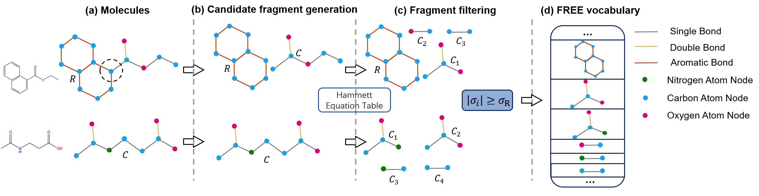
Figure 2: The building process of the FREE Vocabulary.

6.2 The D2L Model

Fig. 3 is to illustrate the motivation of our D2L model, that is, why do we diffuse on two levels — molecule graphs and molecular fragments? The rationale is like this: the structures of real molecules are complex and diverse, and diffusion only at the molecular level cannot capture the real molecular distribution (shown in Fig. 3(a)) well, as shown in Fig. 3(b). Therefore, we perform diffusion on two structural levels: molecules and molecular fragments, with which a mixed Gaussian distribution is obtained, and a better molecular distribution can be obtained, as shown in Fig. 3(c).

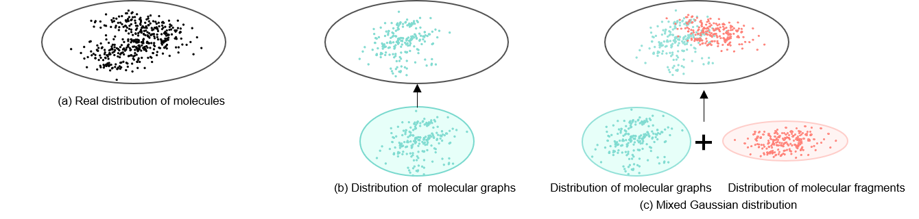
Figure 3: Illustration of the motivation of two-level diffusion.

6.3 Energy Guidance Function

Fig. 4 illustrates how the energy guidance function guides the model to generate molecules of low energy (corresponding to high validity), while discarding molecules of high energy (corresponding to low validity), consequently optimizing the validity of the generated molecules. In our paper, we design the energy guidance function based on molecule validity. Certainly, we can design the energy guidance function for other properties.

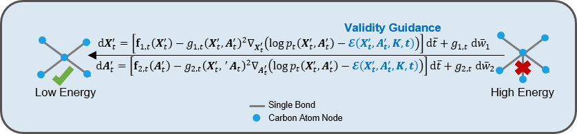
Figure 4: Illustration of energy guidance function for validity optimization.

6.4 Multiple-objective Optimization

Fig. 5 illustrates optimizing two properties (QED and PlogP) simultaneously by Pareto optimal. As described in Sec. 3.5, let $\boldsymbol{\theta}^{*}\in\Omega$, if there is no $\boldsymbol{\theta}\in\Omega$ that makes $\mathcal{L}_{i}(\boldsymbol{\theta})\leq\mathcal{L}_{i}(\boldsymbol{\theta}^{*})$, then $\boldsymbol{\theta}^{*}$ is a solution for the OMP problem. $\mathcal{L}_{i}(\boldsymbol{\theta})\leq\mathcal{L}_{i}(\boldsymbol{\theta}^{*})$ means that $\boldsymbol{\theta}^{*}$ is the best solution without any potential improvement, which is called the Pareto optimal solution. The set of all Pareto optimal solutions $\boldsymbol{\theta}^{*}$ is called the Pareto set, which is denoted as $R_{pa}$. The image of the Pareto set is called the Pareto front ($P_{f}$) , where $P_{f}=\{\mathcal{L}(\boldsymbol{\theta})\}_{\boldsymbol{\theta}\in R_{pa}}$.

In Fig. 5, the molecules from $\mathcal{L}_{i}(\boldsymbol{\theta}^{1})$ to $\mathcal{L}_{i}(\boldsymbol{\theta}^{4})$ constitute the Pareto front, i.e., the optimal solution with regard to the properties QED and Plog, as no other molecules in the space have better QED and PlogP than those in the Pareto front.

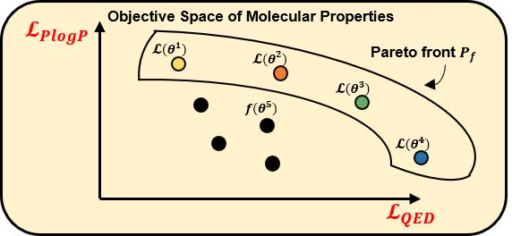
Figure 5: Illustration of 2-property optimization by Pareto Optimal.

7 Algorithm

Alg. 1 outlines the procedure of our method D2L-OMP, which consists of two parts, the diffusion process and the sampling process: the diffusion process aims to simultaneously diffuse at the two levels of molecules and fragments to obtain a mixed Gaussian distribution (Lines 2~5), and the sampling process aims to use the energy-guidance function and multiple -objective mechanisms to optimize the reverse process and sample new molecules from the obtained optimized distribution (Lines 6~15).

Input: A molecular graph $G$, a molecular fragment $\mathcal{F}$, denoising steps $N$, the score function $\boldsymbol{s}(\cdot,t)$

1 begin

2       $\Delta t=\frac{T}{N}$

3       $G_{0}\sim p_{mol}$, $\mathcal{F}_{0}\sim p_{fra}$

4       $G_{T}\leftarrow G_{0},\mathcal{F}_{T}\leftarrow\mathcal{F}_{0}$

5       $G^{\prime}_{T}=G_{T}+\mathcal{F}_{T}$

6       for $i=N$ to $1$ do

7             $t=i\Delta t$

8             $G^{\prime}\sim p_{0t}(G^{\prime}_{t}|G_{0})$ // sample from mixed Gaussian distribution

9             $\mathcal{E}\leftarrow\mathcal{E_{V}}(G^{\prime},K_{V},t)$// calculate the energy function

10             $\mathcal{L}_{OMP}=OMP(\mathcal{L}_{Q},\mathcal{L}_{P})$ // calculate the OMP

11             $F=\mathbf{f}(\boldsymbol{G^{\prime}})-g(\boldsymbol{G^{\prime}})^{2}(s(G^{\prime})-\nabla_{G^{\prime}}\mathcal{E})$

12             $\boldsymbol{z}\sim\mathcal{N}(\mathbf{0},\boldsymbol{I})$ if $i>1$, else $\boldsymbol{z}=\mathbf{0}$

13             $G^{\prime}\leftarrow G^{\prime}-\Delta tF+g(t)\sqrt{\Delta t}\boldsymbol{z}$ // see Eq.(6) for details

14             optimizer.step($\mathcal{L}_{OMP}(G^{\prime})$)

15            

16       end for

17      return $G^{\prime}$

18 end

19

Algorithm 1 The D2L-OMP algorithm.

8 More Experimental Results

8.1 Effects of Parameters

Effect of parameter $\mathrm{W}_{f}$. Tab. 5 shows how the weight of molecular fragments $\mathrm{W}_{f}$ impacts performance on QM9. We can see when $\mathrm{W}_{f}$ is set to 0.01, our D2L-OMP method achieves the best performance.

Effect of the substituent constant threshold $\sigma_{R}$. $\sigma_{R}$ impacts the number of fragments generated by our FREE method. Here, we check the effect of $\sigma_{R}$ on the number of FREE fragments. We choose different values for $\sigma_{R}$, the results are presented in Tab. 6, from which we can see that $\sigma_{R}$ slightly impacts the number of FREE fragments. When the number of fragments is fixed, including as many kinds of fragments as possible will lead to better molecule generation results. In our paper, we set the $R=$hydrogen atom, i.e., using $\sigma_{H}$ as the threshold value.

Effect of parameter $C_{V}$. $C_{V}$ in Eq. (4) is a hyper-parameter to control the optimization strength of the energy guidance function. Here check its effect on QM9, the results are presented in Tab. 7, which shows that our D2L-OMP achieves the best performance when $C_{V}$ is set to 0.1.

Table 5: Effect of parameter $\mathrm{W}_{f}$ on QM9.

$\mathrm{W}_{f}$	Val. w/o corr. (%)↑	Uniqueness (%)↑	FCD ↓
1.0	10.43	96.26	6.53
0.5	93.56	61.89	10.42
0.1	93.33	73.59	10.55
0.01	95.36	74.12	10.41
0.001	92.99	74.10	10.44

Table 6: Results when using different values of threshold $\sigma_{R}$ of FREE.

$\sigma_{R}$	#fragments
R=hydrogen atom	3908
R=Fluoro atom	3907
R=Cyano	3894
R=Nitro	3890
R=Methoxy	3989
R=Methyl	3902
R=Hydroxy	3898

Table 7: Effect of parameter $C_{V}$ on QM9.

$C_{V}$	Val. w/o corr. (%)↑	Uniqueness (%)↑	FCD ↓
1.0	99.64	95.97	3.98
0.5	99.40	97.50	3.43
0.1	98.60	99.80	2.77
0.01	98.55	97.47	3.35
0.001	98.57	97.47	3.36

8.2 Property Distribution of Generated Molecules

Here, we compare property (QED and PlogP) distributions of 10,000 generated molecules by different models. The results are shown in Fig. 7 and Fig. 7, from which we can see that the property distributions of molecules generated by our D2L-OPM method is closer to the property distributions of the datasets than the other models in most cases.

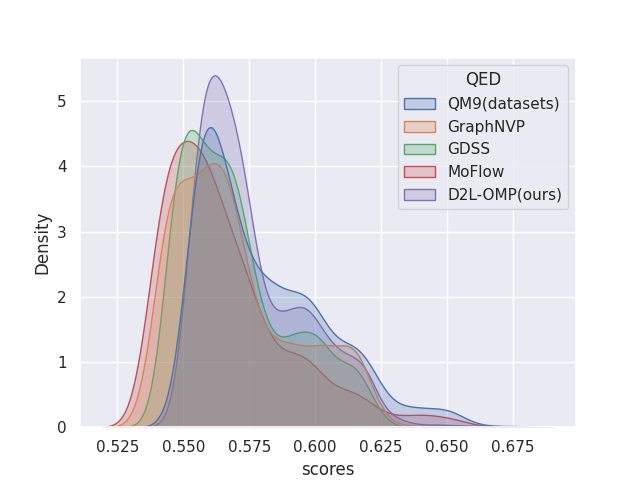
(a) QED

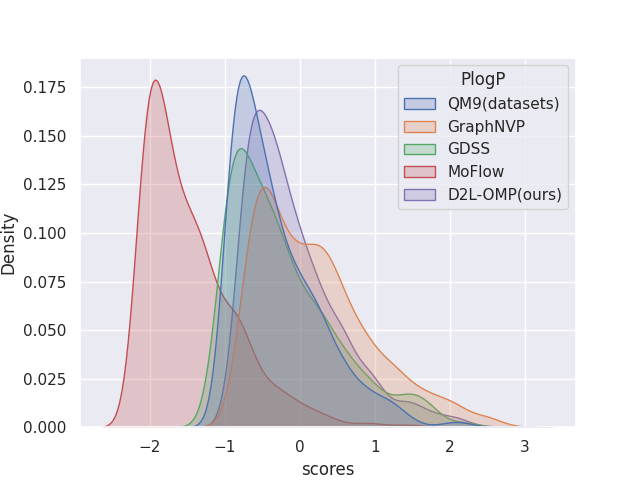
(b) PlogP

Figure 6: Property Distributions of 10,000 molecules generated by different models on QM9.

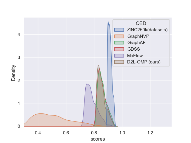
(a) QED

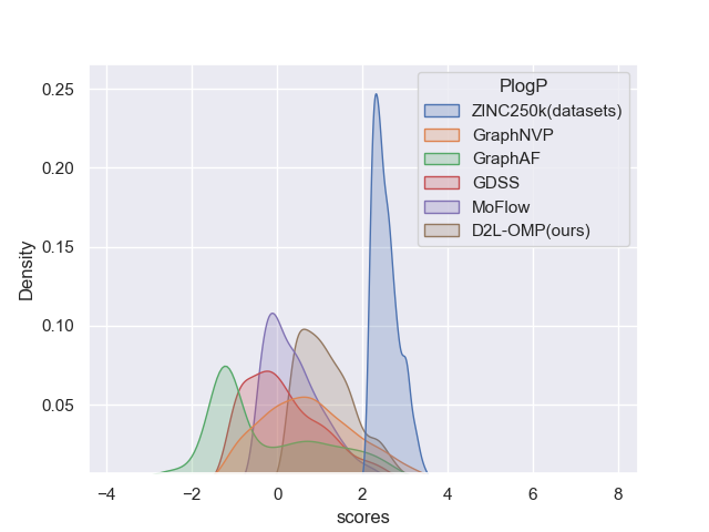
(b) PlogP

Figure 7: Property Distributions of 10,000 molecules generated by different models on ZINC250k.

8.3 Visualization of Generated Molecules

Fig. 8 and Fig. 9 show 50 randomly selected molecules generated by our method on QM9 and ZINC250k, respectively.

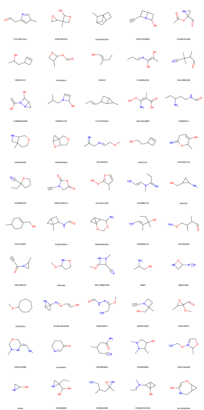
Figure 8: Visualization of 50 randomly-selected molecules generated by our model on QM9.

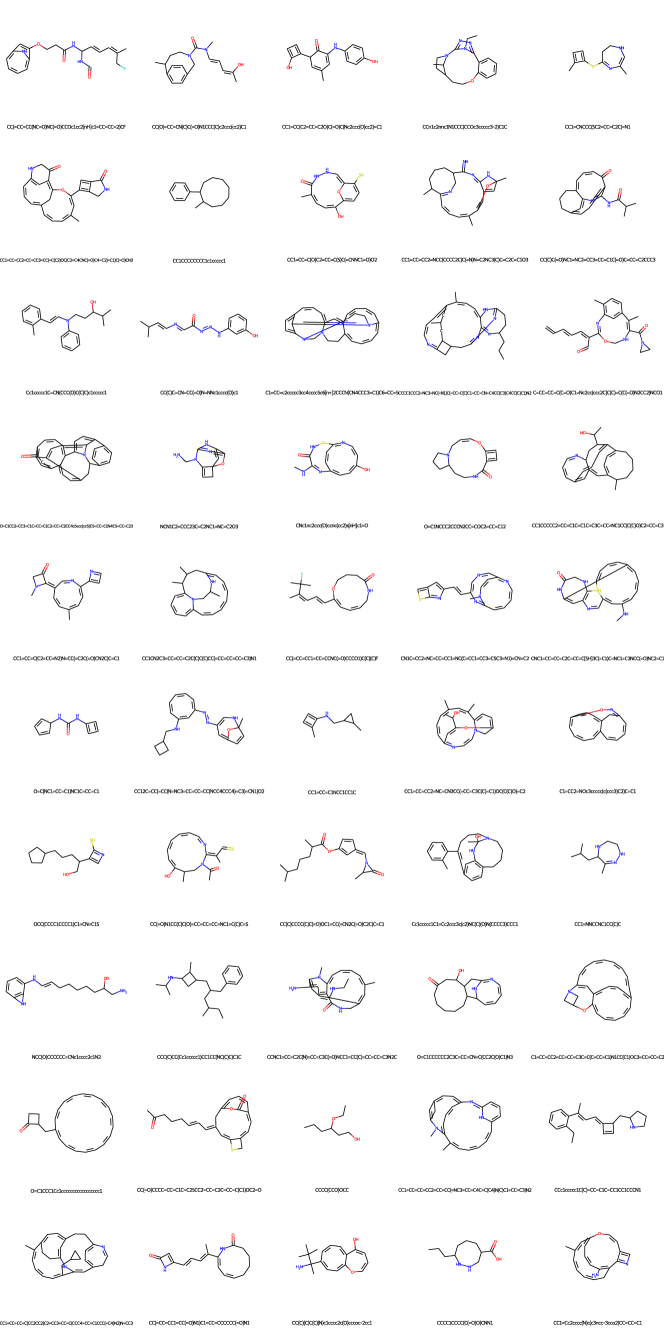
Figure 9: Visualization of 50 randomly-selected molecules generated by our model on ZINC250k.

9 Model Implementation Details

Our method is implemented under PyTorch. The score-based model $\boldsymbol{s}_{\theta}(\cdot,t)$ is implemented with 3 GCN layers, and the hidden dimension is set as 16. $\boldsymbol{s}_{\psi}(\cdot,t)$ is implemented with 3 GCN layers on QM9 and 6 GCN layers on ZINC250k. The hidden dimension of $\boldsymbol{s}_{\psi}(\cdot,t)$ is set to 16. Our model is trained with a batch size of 1024 on GeForce RTX 3090 GPU. We train the model on QM9 for 300 epochs and on ZINC250k for 500 epochs. We optimize our model by Adam with a fixed learning rate of 0.005.

10 Impacts and Limitations

Impacts. In this paper we propose a novel model for generating molecules with multiple desirable properties. Our method is an expanded diffusion model with multiple innovative designs, including diffusing on two molecular structural levels — molecules and fragments, optimizing multiple properties simultaneously, and fragmenting molecules based on electronic effect. Extensive experiments show that our method can generate molecules with better properties, including validity, uniqueness, novelty, FCD, QED and PlogP, than those generated by existing models. Our work pioneers a new way to molecule generation, thus is of considerable significance to drug design and discovery.

Limitations. Our method is an expanded diffusion model, integrating with multiple-objective optimization. Both the diffusion model and multiple-objective optimization are relatively time-consuming. So in the future, we will explore efficient diffusion models and multiple-objective optimization algorithms. Furthermore, here we optimize three properties simultaneously. But molecules have many properties. So as future work, we will try to optimize more properties simultaneously.

References

- [1] Bernard H Munos and William W Chin. How to revive breakthrough innovation in the pharmaceutical industry. Science translational medicine, 3(89):89cm16–89cm16, 2011.
- [2] Steven M Paul, Daniel S Mytelka, Christopher T Dunwiddie, Charles C Persinger, Bernard H Munos, Stacy R Lindborg, and Aaron L Schacht. How to improve r&d productivity: the pharmaceutical industry’s grand challenge. Nature reviews Drug discovery, 9(3):203–214, 2010.
- [3] David Weininger, Arthur Weininger, and Joseph L Weininger. Smiles. 2. algorithm for generation of unique smiles notation. Journal of chemical information and computer sciences, 29(2):97–101, 1989.
- [4] Chengxi Zang and Fei Wang. Moflow: an invertible flow model for generating molecular graphs. In Proceedings of the 26th ACM SIGKDD International Conference on Knowledge Discovery & Data Mining, pages 617–626, 2020.
- [5] Rafael Gómez-Bombarelli, Jennifer N Wei, David Duvenaud, José Miguel Hernández-Lobato, Benjamín Sánchez-Lengeling, Dennis Sheberla, Jorge Aguilera-Iparraguirre, Timothy D Hirzel, Ryan P Adams, and Alán Aspuru-Guzik. Automatic chemical design using a data-driven continuous representation of molecules. ACS central science, 4(2):268–276, 2018.
- [6] Jörg Degen, Christof Wegscheid-Gerlach, Andrea Zaliani, and Matthias Rarey. On the art of compiling and using’drug-like’chemical fragment spaces. ChemMedChem: Chemistry Enabling Drug Discovery, 3(10):1503–1507, 2008.
- [7] Raghunathan Ramakrishnan, Pavlo O Dral, Matthias Rupp, and O Anatole Von Lilienfeld. Quantum chemistry structures and properties of 134 kilo molecules. Scientific data, 1(1):1–7, 2014.
- [8] John J Irwin, Teague Sterling, Michael M Mysinger, Erin S Bolstad, and Ryan G Coleman. Zinc: a free tool to discover chemistry for biology. Journal of chemical information and modeling, 52(7):1757–1768, 2012.
- [9] Wengong Jin, Regina Barzilay, and Tommi Jaakkola. Junction tree variational autoencoder for molecular graph generation. In International conference on machine learning, pages 2323–2332. PMLR, 2018.
- [10] Kaushalya Madhawa, Katushiko Ishiguro, Kosuke Nakago, and Motoki Abe. Graphnvp: An invertible flow model for generating molecular graphs. arXiv preprint arXiv:1905.11600, 2019.
- [11] Chence Shi, Minkai Xu, Zhaocheng Zhu, Weinan Zhang, Ming Zhang, and Jian Tang. Graphaf: a flow-based autoregressive model for molecular graph generation. arXiv preprint arXiv:2001.09382, 2020.
- [12] Youzhi Luo, Keqiang Yan, and Shuiwang Ji. Graphdf: A discrete flow model for molecular graph generation. In International Conference on Machine Learning, pages 7192–7203. PMLR, 2021.
- [13] Jaehyeong Jo, Seul Lee, and Sung Ju Hwang. Score-based generative modeling of graphs via the system of stochastic differential equations. In International Conference on Machine Learning, pages 10362–10383. PMLR, 2022.
- [14] Clement Vignac, Igor Krawczuk, Antoine Siraudin, Bohan Wang, Volkan Cevher, and Pascal Frossard. Digress: Discrete denoising diffusion for graph generation. arXiv preprint arXiv:2209.14734, 2022.
- [15] Gabriel Lima Guimaraes, Benjamin Sanchez-Lengeling, Carlos Outeiral, Pedro Luis Cunha Farias, and Alán Aspuru-Guzik. Objective-reinforced generative adversarial networks (organ) for sequence generation models. arXiv preprint arXiv:1705.10843, 2017.
- [16] Nicola De Cao and Thomas Kipf. Molgan: An implicit generative model for small molecular graphs. arXiv preprint arXiv:1805.11973, 2018.
- [17] Andrew E Blanchard, Christopher Stanley, and Debsindhu Bhowmik. Using gans with adaptive training data to search for new molecules. Journal of cheminformatics, 13(1):1–8, 2021.
- [18] Martin Simonovsky and Nikos Komodakis. Graphvae: Towards generation of small graphs using variational autoencoders. In Artificial Neural Networks and Machine Learning–ICANN 2018: 27th International Conference on Artificial Neural Networks, Rhodes, Greece, October 4-7, 2018, Proceedings, Part I 27, pages 412–422. Springer, 2018.
- [19] Qi Liu, Miltiadis Allamanis, Marc Brockschmidt, and Alexander Gaunt. Constrained graph variational autoencoders for molecule design. Advances in neural information processing systems, 31, 2018.
- [20] Bidisha Samanta, Abir De, Gourhari Jana, Vicenç Gómez, Pratim Kumar Chattaraj, Niloy Ganguly, and Manuel Gomez-Rodriguez. Nevae: A deep generative model for molecular graphs. The Journal of Machine Learning Research, 21(1):4556–4588, 2020.
- [21] Diederik P Kingma and Max Welling. Auto-encoding variational bayes. arXiv preprint arXiv:1312.6114, 2013.
- [22] Meng Liu, Keqiang Yan, Bora Oztekin, and Shuiwang Ji. Graphebm: Molecular graph generation with energy-based models. arXiv preprint arXiv:2102.00546, 2021.
- [23] Yilun Du and Igor Mordatch. Implicit generation and modeling with energy based models. Advances in Neural Information Processing Systems, 32, 2019.
- [24] G.L. Miessler, P.J. Fischer, and D.A. Tarr. Inorganic Chemistry. Pearson advanced chemistry series. Pearson, 2014.
- [25] Louis P Hammett. The effect of structure upon the reactions of organic compounds. benzene derivatives. Journal of the American Chemical Society, 59(1):96–103, 1937.
- [26] IUPAC IUPAC. Compendium of chemical terminology. the “Gold Book.” Blackwell Scientific Publications Oxford, 1997.
- [27] Sheue L Keenan, Karl P Peterson, Kelly Peterson, and Kyle Jacobson. Determination of hammett equation rho constant for the hydrolysis of p-nitrophenyl benzoate esters. Journal of chemical education, 85(4):558, 2008.
- [28] Yann LeCun, Sumit Chopra, Raia Hadsell, M Ranzato, and Fujie Huang. A tutorial on energy-based learning. Predicting structured data, 1(0), 2006.
- [29] Pascal Vincent. A connection between score matching and denoising autoencoders. Neural computation, 23(7):1661–1674, 2011.
- [30] Yang Song, Jascha Sohl-Dickstein, Diederik P Kingma, Abhishek Kumar, Stefano Ermon, and Ben Poole. Score-based generative modeling through stochastic differential equations. arXiv preprint arXiv:2011.13456, 2020.
- [31] Jinheon Baek, Minki Kang, and Sung Ju Hwang. Accurate learning of graph representations with graph multiset pooling. arXiv preprint arXiv:2102.11533, 2021.
- [32] William B. T. Mock. Pareto Optimality, pages 808–809. Springer Netherlands, Dordrecht, 2011.
- [33] Harold W Kuhn and Albert W Tucker. Nonlinear programming. In Traces and emergence of nonlinear programming, pages 247–258. Springer, 2013.
- [34] Jean-Antoine Désidéri. Multiple-gradient descent algorithm (mgda) for multiobjective optimization. Comptes Rendus Mathematique, 350(5-6):313–318, 2012.
- [35] Greg Landrum et al. Rdkit: Open-source cheminformatics software. 2016. URL http://www. rdkit. org/, https://github. com/rdkit/rdkit, 149(150):650, 2016.
- [36] Kristina Preuer, Philipp Renz, Thomas Unterthiner, Sepp Hochreiter, and Gunter Klambauer. Fréchet chemnet distance: a metric for generative models for molecules in drug discovery. Journal of chemical information and modeling, 58(9):1736–1741, 2018.
- [37] G Richard Bickerton, Gaia V Paolini, Jérémy Besnard, Sorel Muresan, and Andrew L Hopkins. Quantifying the chemical beauty of drugs. Nature chemistry, 4(2):90–98, 2012.
- [38] Ziqiao Zhang, Jihong Guan, and Shuigeng Zhou. Fragat: a fragment-oriented multi-scale graph attention model for molecular property prediction. Bioinformatics, 37(18):2981–2987, 2021.
- [39] Ailin Xie, Ziqiao Zhang, Jihong Guan, and Shuigeng Zhou. Self-supervised learning with chemistry-aware fragmentation for effective molecular property prediction. Briefings in Bioinformatics, 24(5):bbad296, 2023.
- [40] Soojung Yang, Doyeong Hwang, Seul Lee, Seongok Ryu, and Sung Ju Hwang. Hit and lead discovery with explorative rl and fragment-based molecule generation. Advances in Neural Information Processing Systems, 34:7924–7936, 2021.