Extended superposition theorem under power grid topological changes

Abstract

Standard superposition theorem has been the basis in the last decades for many power system problems decomposition involving changes in nodal injections, from productions and loads. Its application scope has however been limited to fixed grid topology and breaks as soon as a topology change happens in the grid. For instance, it cannot be applied to compute N-2 power flows simply from N-1 security analysis. Topological changes also become a flexibility used more and more frequently for congestion management. Studying the effect of combinatorial topological changes is hence of interest, but so far very computation intensive. In this paper, we propose an extension of the superposition theorem to varying grid topologies. We demonstrate it under the DC approximation for all topological changes, namely line disconnection and reconnection, bus splitting and merging. We finally apply it to two use cases related to the above mentioned, effectively extending its scope of application.

I Introduction

Superposition theorem (ST) in electrical circuit is a century-old scientific foundation presented in every reference textbook [1]. It has helped make tremendous progress in the design, analysis and control of electrical circuits, with regards to power flows in power grids in particular. But so far, it has not been explicitly extended to electrical circuits with changing topologies. At the time of steep Energy Transition requiring more flexible operations [2], topological changes such as node splitting will happen more frequently. Tools with better performance under these conditions are needed [3]. Such changes usually requires to recompute the costly underlying matrix factorization of classical power flow methods. Our ST extension aims at bypassing this computation.

There exists preliminary work in the direction of this extended ST in the form of Line Outage Distribution Factors (LODFs) [4, 5, 6]. Indeed [7] first proposed generalized LODF for multiple outages to be computed in an efficient form by solving a system of linear equations in the dimension of line outages. Bus Splitting Distribution Factors (BSDFs) were proposed lately [8] to compute unitary bus splitting change from PTDF. Yet none of these works make the connection with an underlying ST and only deal with specific cases.

In the following, we propose to first extend ST to line reconnection, bus splitting and merging. We further unify them under a single extended ST, using only minimal necessary information. Instead of a pure calculus demonstration as in previous works, we rely mostly on grid equivalent model interplay as well on the existing ST. This comes with interpretability benefit. Every kind of topological change can eventually fall into a joint and unique linear system to solve in the dimension of unitary changes.

We finally share numerical results of the extended ST implementation, to show its equivalence to power flow solvers in terms of accuracy under all topological change canonical cases. We finally run experiments over two applications, namely security analysis following a topological change and topological remedial action search. We analyze the gains of this method in terms of speed-up and interpretability with comparison to existing baseline methods.

II Extended Superposition theorem

TABLE I: Notation

symbols
$\setminus l$	line $l$ disconnected
$=l$	line $l$ reconnected
$\odot$	composition symbol
Sets
$C$	set of lines $l$ to reconnect
$O$	set of lines $l$ in outage
$C_{\setminus o}$	set of lines $l$ to reconnect except line $o$
$C_{1,2}$ or $C_{1,2,3}$	set of 2 or 3 lines $l$ to reconnect
$O_{1,2}$ or $O_{1,2,3}$	set of 2 or 3 lines $l$ in outage
Variables
T	a grid topology
$\mathrm{\textit{T}}^{ref}$	reference grid topology to start from
$\mathrm{\textit{T}}^{tgt}$	target topology reached after changes
$\mathrm{\textit{T}}_{O}$	topology with $l\in O$ lines disconnected
$\mathrm{\textit{T}}_{C}$	topology with $l\in C$ lines reconnected
$\tau_{k}$	$k^{th}$ unitary topology change
$\tau_{\setminus l}$	unitary line $l$ disconnection
$\tau_{=l}$	unitary line $l$ reconnection
$\mathrm{\textit{T}}^{\tau_{k}}$	grid topology $\mathrm{\textit{T}}^{ref}\odot\tau_{k}$ after
	applying $\tau_{k}$ to $\mathrm{\textit{T}}^{ref}$
Bbus	nodal injection vector
$Bbus^{ref}$	reference nodal injection vector
$\delta Bbus^{k}$	$k^{th}$ unitary change from $Bbus^{ref}$
$PF(Bbus,\mathrm{\textit{T}})$	lines power flow under Bbus injections
	and topology T with DC approximation
$PF(\mathrm{\textit{T}})$	lines power flow under $Bbus^{ref}$
	injections and topology T
$pf^{\mathrm{\textit{T}}}_{l}$	line $l$ flow under $Bbus^{ref}$ injections
	and topology T
$cf^{T}_{l}$	equivalent line $l$ cancelling flow in T
$Bcf^{T}_{l}$	$cf^{T}_{l}$ in nodal injection vector form
$Bcf^{T}$	sum of $Bcf^{T}_{l}$ nodal injection vectors
$vf^{T}_{l}$	line $l$ virtual induced flow in T
$\Theta^{\mathrm{\textit{T}}}_{l_{or}},\Theta^{\mathrm{\textit{T}}}_{l_{ex}},\Delta\Theta^{\mathrm{\textit{T}}}_{l}$	phases & difference at line $l$ extremities
	for $Bbus^{ref}$ injections & topology T
$Ifo^{\mathrm{\textit{T}}^{\tau_{k}}}_{i}$	some state information on $i^{th}$ asset
	of interest in topology $\mathrm{\textit{T}}^{\tau_{k}}$
$LODF_{o,l}$	line outage $o$ distribution factor
	on line $l$ in $\mathrm{\textit{T}}^{ref}$
$\alpha$ and $\beta^{k}$	extended ST theorem scalar coefficients
	to $PF(T^{ref})$ and $PF(T^{\tau_{k}})$
$\alpha_{C},\beta^{k}_{C}$ / $\alpha_{O},\beta^{k}_{O}$	coefficients in reco / disconnections
Parameters
$N_{\tau},N_{O},N_{C}$	$card(\{\tau_{k}\}),card(O),card(C)$
$\sigma_{l}$	conductance of line l

We consider a grid with production and loads at electrical bus bar nodes, represented by the nodal injection vector $Bbus$, and branches connected under a given grid topology we denote by T. Our aim is to compute power flows $PF(Bbus,\mathrm{\textit{T}})$. We will restrict ourself in this paper to the DC approximation [9] and work under the assumption that the grid remains connected and does not get split apart in multiple components.

II-A Definition

Given a linear combination of changes in nodal injection vectors $\delta Bbus^{i}$ that adds up to a reference nodal injection vector $Bbus^{ref}$ to sum up to a target vector $Bbus^{tgt}$, the standard ST decomposes the resulting grid state, namely a power flow $PF(Bbus^{tgt},\mathrm{\textit{T}})$, as the linear combination of grid states of single input elements for a fixed grid topology T:

$$PF(Bbus^{tgt},\mathrm{\textit{T}})=PF(Bbus^{ref},\mathrm{\textit{T}})+\sum_{i}PF(\delta Bbus^{i},\mathrm{\textit{T}})\\ \text{with }Bbus^{tgt}=Bbus^{ref}+\sum_{i}\delta Bbus^{1}$$ (1)

This superposition theorem have proven very useful to decompose the problem analytically, allowing for either more efficient computations or better interpretability when analyzing some grid phenomena. We aim at transposing this handy tool to topological changes, eg. change in the topology T.

Similarly we propose to extend it in the following to topological changes. Starting from $\mathrm{\textit{T}}_{ref}$ as the reference topology to which we apply topological changes $\tau_{i}$ in indifferent order, we reach a target topology $\mathrm{\textit{T}}^{tgt}$. In this case, as illustrated in Figure 1, we will demonstrate the following extended ST:

$$PF(Bbus^{ref},\mathrm{\textit{T}}^{tgt})=\alpha PF(Bbus^{ref},\mathrm{\textit{T}}^{ref})+$$

$$\sum_{i}\beta^{i}PF(Bbus^{ref},\mathrm{\textit{T}}^{\tau_{i}})$$

$$\text{with }\mathrm{\textit{T}}^{tgt}=\mathrm{\textit{T}}^{ref}\odot\tau_{1}\odot...\odot\tau_{N_{\tau}}\text{ and }\alpha=1-\sum_{i}\beta^{i}$$

Note that this decomposition is a weighted linear combination instead of a pure linear one as before. This requires to compute these weights. Finding the betas stems from solving a linear system of dimension the number of considered changes $N_{\tau}$. Yet only minimal information is needed for this:

• $\text{Ifo}^{T^{ref}}_{l}$, resp. $\text{Ifo}^{T^{\tau_{k}}}_{l}$, as state variables from reference power flow state $PF(T^{ref})$, resp. from each unitary topological change $PF(\mathrm{\textit{T}}^{\tau_{k}})$ state, as in the ST equation.

• the nature of $\tau_{k}$, which assets are impacted by it and how.

Beyond this, no other knowledge such as underlying grid properties, complete adjacency matrix or complete topology information is needed.

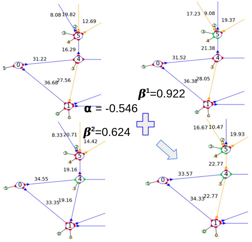
Figure 1: Extended ST example on IEEE14, starting from a meshed topology (top left) to which you apply 2 node splitting actions at substations 4 and 5 (bottom right). Displayed ST coefficients are derived from initial and unitary action states.

We will eventually demonstrate that the linear system to solve for computing the beta coefficients is of the form :

$$\begin{bmatrix}1&1-\frac{\text{Ifo}^{\mathrm{\textit{T}}^{\tau_{2}}}_{l_{1}}}{\text{Ifo}^{\mathrm{\textit{T}}^{ref}}_{l_{1}}}&...&1-\frac{\text{Ifo}^{\mathrm{\textit{T}}^{\tau_{n}}}_{l_{1}}}{\text{Ifo}^{\mathrm{\textit{T}}^{ref}}_{l_{1}}}\\ 1-\frac{\text{Ifo}^{\mathrm{\textit{T}}^{\tau_{1}}}_{l_{2}}}{\text{Ifo}^{\mathrm{\textit{T}}^{ref}}_{l_{2}}}&1&...&1-\frac{\text{Ifo}^{\mathrm{\textit{T}}^{\tau_{n}}}_{l_{2}}}{\text{Ifo}^{\mathrm{\textit{T}}^{ref}}_{l_{2}}}\\ ...&...&...&...\\ 1-\frac{\text{Ifo}^{\mathrm{\textit{T}}^{\tau_{1}}}_{l_{n}}}{\text{Ifo}^{\mathrm{\textit{T}}^{ref}}_{l_{n}}}&1-\frac{\text{Ifo}^{\mathrm{\textit{T}}^{\tau_{2}}}_{l_{n}}}{\text{Ifo}^{\mathrm{\textit{T}}^{\tau_{2}}}_{l_{n}}}&...&1\\ \end{bmatrix}\begin{bmatrix}\beta 1\\ \beta 2\\ ...\\ \beta n\end{bmatrix}=\begin{bmatrix}1\\ 1\\ ...\\ 1\end{bmatrix}$$ (2)

$\text{Ifo}^{\mathrm{\textit{T}}}_{l_{i}}$ is either $pf^{\mathrm{\textit{T}}}_{l_{i}}$ or $\Delta\theta^{\mathrm{\textit{T}}}_{l_{i}}$ depending on the nature of $\tau_{k}$.

II-B two equivalent models

We now describe an equivalent grid state model for disconnected lines that will be the foundation for extended ST demonstrations. Disconnecting a line leading to Topology $\mathrm{\textit{T}}_{O}$ is actually equivalent of virtually injecting a cancelling flow $cf_{l}^{\mathrm{\textit{T}}_{O}}$ (or $Bcf^{\mathrm{\textit{T}}_{O}}_{l}$ in nodal injection vector form) at that line $l$ [7, 10] while keeping this line, as well as other lines to disconnect, virtually connected as in Figure 2. Given $N_{O}$ disconnected lines from $\mathrm{\textit{T}}^{ref}$, this equivalence can be represented by:

$$PF(Bbus^{ref},\mathrm{\textit{T}}_{O})=PF(Bbus^{ref}+\sum_{l\in O}Bcf^{\mathrm{\textit{T}}_{O}}_{l},\mathrm{\textit{T}}^{ref})$$ (3)

The grid topology in the virtual injection model is hence $\mathrm{\textit{T}}^{ref}$ as the lines remain virtually connected.

These models are equivalent in that they result in the same power flows. Phases at nodes also remain the same under the same reference phase node. Indeed, as a quick check, all connected line flows remains the same, hence the difference of phases $\Delta\theta_{l}$ at their extremity remain the same. From the reference node, applying identical phase difference hops by hops to neighboring line extremities gives you the same phases for each nodes eventually.

In this equivalent model, there exist a ohm’s law induced virtual power flow $vf^{\mathrm{\textit{T}}_{O}}_{l}$ at line $l$ still virtually connected:

$$vt_{l}^{\mathrm{\textit{T}}_{O}}=\sigma_{l}\Delta\theta_{l}^{\mathrm{\textit{T}}_{O}}$$ (4)

This is based on the fact that phases remain the same in the disconnected case and virtually connected case. The related flows to virtual injections $Bcf^{\mathrm{\textit{T}}_{O}}$ cancel $vf^{\mathrm{\textit{T}}_{O}}_{l}$ out in the end.

II-C Line disconnections

Let’s first consider the restricted topological changes case of line disconnections $o\in O$. We depart from a reference topology in which those lines are connected $\mathrm{\textit{T}}^{ref}_{C}$ and reach a topology $\mathrm{\textit{T}}^{tgt}_{O}$ with all lines disconnected. The proposed extended ST in this case has been already indirectly demonstrated in Generalize LODF paper [7]. Indeed they compute multi-outage power flow solving a linear system of LODF, which is composed of reference and unitary outage power flow states. However our new demonstration from scratch here will pave the way for the next demonstrations too.

To derive the linear system of equations to solve, that will further (re)demonstrate the extended ST theorem, we work with the equivalent virtual injection models. In the one-line disconnection case, the cancelling flow in this model is $cf_{l}^{\mathrm{\textit{T}}^{\tau_{\setminus l}}}=-pf_{l}^{\mathrm{\textit{T}}^{ref}}=-vt_{l}^{\mathrm{\textit{T}}^{\tau_{\setminus l}}}$.

In the multiple line disconnection case, virtually injected cancelling flows on other lines to disconnect (but virtually connected in the equivalent model) induce additional virtual flows on the line of interest as can be derived from standard ST(1):

$$\begin{split}PF(B_{bus}^{ref},\mathrm{\textit{T}}_{O}^{tgt})&=PF(B_{bus}^{ref}+\sum_{l\in O}Bcf^{\mathrm{\textit{T}}_{O}^{tgt}}_{l},\mathrm{\textit{T}}^{ref})\\ &=PF(B_{bus}^{ref},\mathrm{\textit{T}}^{ref})+\sum_{l\in O}PF(Bcf^{\mathrm{\textit{T}}_{O}^{tgt}}_{l},\mathrm{\textit{T}}^{ref})\end{split}$$ (5)

To derrive the new powerflow terms, We will make use of line outage distributions factors aka LODFs:

$$LODF_{o,l}=\frac{pf_{l}^{\mathrm{\textit{T}}^{\tau_{\setminus o}}}-pf_{l}^{ref}}{pf_{o}^{ref}}$$ (6)

Note that LODF remain constant for a given topology such as $\mathrm{\textit{T}}^{ref}$. In the equivalent modeling, as its topology is $\mathrm{\textit{T}}^{ref}$, we can hence reuse the same LODF computed in the reference topology.

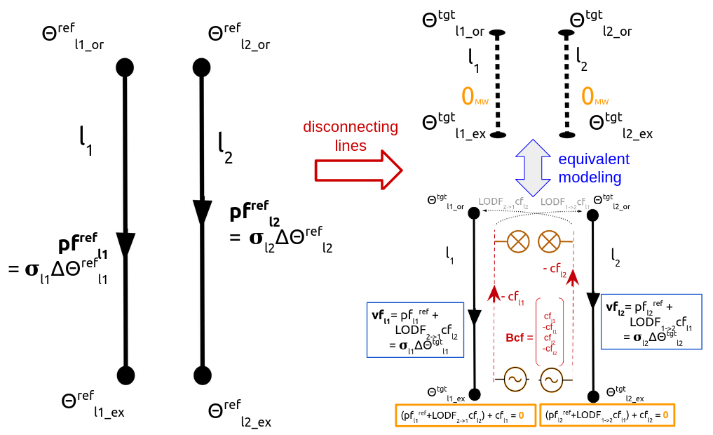
Figure 2: Left, Power Flow in the reference topology for the two lines to disconnect. Right, the two lines disconnected with two equivalent models: the usual one with physical line disconnections on top, and the cancelling flow model at the bottom with lines still virtually connected

Using $LODF$, $PF(Bcf^{\mathrm{\textit{T}}_{O}^{tgt}}_{l},\mathrm{\textit{T}}^{ref})$ is simply:

$$PF(Bcf^{\mathrm{\textit{T}}_{O}^{tgt}}_{l},\mathrm{\textit{T}}^{ref})=LODF_{l}\times cf_{l}^{\mathrm{\textit{T}}_{O}^{tgt}}$$ (7)

Which eventually leads by substitution to the equation:

$$PF(B_{bus}^{ref},\mathrm{\textit{T}}_{O}^{tgt})=PF(B_{bus}^{ref},\mathrm{\textit{T}}^{ref}_{C})+\sum_{l\in O}LODF_{l}\times cf_{l}^{\mathrm{\textit{T}}_{O}^{tgt}}$$ (8)

As $pf_{l}^{\mathrm{\textit{T}}_{O}}=0$ for disconnected lines, this lead to the system of $N_{o}$ independant cancelling flow equations:

$$pf_{l}^{ref}+\sum_{o\in O}LODF_{o,l}\times cf_{o}^{\mathrm{\textit{T}}_{O}}=0\text{ for all }l\in O$$ (9)

The virtual induced flow $vt_{l}$ on line $l$ is then:

$$vf_{l}^{\mathrm{\textit{T}}_{O}}=pf_{l}^{ref}+\sum_{o\in O,o\neq l}LODF_{o,l}\times cf_{o}^{\mathrm{\textit{T}}_{O}}\\$$ (10)

From the initial flow $pf_{l}^{ref}$, the contribution of other cancelling flows are added up to result in this induced flow. Given LODF definition from (6) the extended ST is:

$$\begin{split}PF(\mathrm{\textit{T}}_{O}^{tgt})&=PF(\mathrm{\textit{T}}^{ref}_{C})+\sum_{l\in O}(PF(\mathrm{\textit{T}}^{\tau_{\setminus l}})-PF(\mathrm{\textit{T}}^{ref}_{C}))\frac{cf_{l}^{\mathrm{\textit{T}}_{O}^{tgt}}}{pf_{l}^{\mathrm{\textit{T}}^{ref}_{C}q}}\\ &=\alpha\times PF(\mathrm{\textit{T}}^{ref}_{C})+\sum_{l\in O}\beta^{l}\times PF(\mathrm{\textit{T}}^{\tau_{\setminus l}})\end{split}\\ \text{with }\alpha=(1-\sum_{l\in O}\frac{cf_{l}^{\mathrm{\textit{T}}_{O}^{tgt}}}{pf_{l}^{\mathrm{\textit{T}}^{ref}_{C}}})\text{ and }\beta^{l}=\frac{cf_{l}^{\mathrm{\textit{T}}_{O}^{tgt}}}{pf_{l}^{\mathrm{\textit{T}}^{ref}_{C}}}$$ (11)

where we find that:

$$\alpha=1-\sum_{l\in O}\beta^{l}$$ (12)

Substituting $\beta^{l}$ for $cf_{l}^{\mathrm{\textit{T}}_{O}^{tgt}}$ in (9), we have:

$$pf_{l}^{ref}+\sum_{o\in O}LODF_{o,l}\times\beta^{o}pf_{o}^{ref}=0\text{ for all }l\in O$$ (13)

And reusing LODF definition from (6) we recover (2):

$$pf_{l}^{ref}=\beta^{l}\times pf_{l}^{ref}+\sum_{o\in O,o\neq l}(\frac{pf_{l}^{ref}-pf_{l}^{\mathrm{\textit{T}}^{\tau_{\setminus o}}}}{pf_{o}^{ref}})\beta^{o}pf_{o}^{ref}\\ 1=\beta^{l}\times 1+\sum_{o\in O,o\neq l}(1-\frac{pf_{l}^{\mathrm{\textit{T}}^{\tau_{\setminus o}}}}{pf_{l}^{ref}})\beta^{o}\text{ for all }l\in O$$ (14)

We see from (8) or (11) that it solely relies here on reusing known quantities $PF(\mathrm{\textit{T}}^{ref})$, $PF(\mathrm{\textit{T}}^{\tau_{\setminus o}})$ (or $LODF$ equivalently), and requires to solve an additional linear system of equations of the size of the number of topological changes, that is the number of line disconnections here.

II-D Line reconnections

In this section, we are considering line reconnections $\tau_{=l}$ topological changes from a reference topology $\mathrm{\textit{T}}^{ref}_{O}$ in which those lines were initially not connected. So we are changing state in a reverse order from Figure 2: the initial state is the one with disconnected lines as on the right and the final state is with connected lines as on the left. Here we cannot really reuse the linear system (9) as is, as there is not equivalent of $pf^{ref}_{l}$ for initially disconnected lines $l$ in this case. However we can reuse the extended ST for line disconnections from previous section II-C, to prove it for reconnections such that:

$$PF(\mathrm{\textit{T}}_{C}^{tgt})=\alpha_{C}PF(\mathrm{\textit{T}}^{ref}_{O})+\sum_{l_{i}\in C}\beta_{C}^{l_{i}}PF(\mathrm{\textit{T}}^{\tau_{=l_{i}}}_{O})\\ \text{with }\alpha_{C}=1-\sum_{l_{i}\in C}\beta_{C}^{l_{i}}$$ (15)

II-D1 Demonstration

We first demonstrate that if the ST exists, there is a unique decomposition, and them show its existence.

Unicity

From (15), we can deduce that the $\beta$ coefficient would have a unique value as simple as:

$$\beta_{C}^{l_{i}}=\frac{pf^{l_{i}}_{{}_{\mathrm{\textit{T}}_{C}^{tgt}}}}{pf^{l_{i}}_{\mathrm{\textit{T}}^{\tau_{=l_{i}}}_{O}}}$$ (16)

This stems from the fact that flow at line $l_{i}$ is non null only in topologies $\mathrm{\textit{T}}_{C}^{tgt}$ and $\mathrm{\textit{T}}^{\tau_{=l_{i}}}_{O}$ in which the line is connected. For all the other topologies, $l_{i}$ is disconnected with null flow. Hence all other terms for $l_{i}$ index are null in extended ST for line reconnections.

Even if we have not yet computed $pf^{l_{i}}_{{}_{\mathrm{\textit{T}}_{C_{1,2,3}}^{tgt}}}$, this proves the uniqueness of $\beta$ coefficients, as well as $\alpha$ by transitivity, given the uniqueness of powerflows.

Existence

two line reconnections case We can start by reusing (11) with reverse roles of reference and target topologies:

$$PF(\mathrm{\textit{T}}^{ref}_{O_{1,2}})=\alpha_{O_{1,2}}\times PF(\mathrm{\textit{T}}_{C_{1,2}}^{tgt})+\sum_{i\in\{1,2\}}\beta^{l_{i}}_{O_{1,2}}\times PF(\mathrm{\textit{T}}^{\tau_{\setminus l_{i}}}_{C_{1,2}})$$ (17)

This time $PF(\mathrm{\textit{T}}_{C_{1,2}}^{tgt})$ is the superposed state we are looking for. In the 2 lines reconnection case, the unitary reconnection grid topologies $\mathrm{\textit{T}}^{\tau_{=l}}_{O_{1,2}}$ are the same as the unitary disconnection $\mathrm{\textit{T}}^{\tau_{\setminus l}}_{C_{1,2}}$ as $\mathrm{\textit{T}}^{ref}_{C_{1,2}}\circ\tau_{\setminus l}=\mathrm{\textit{T}}^{ref}_{O_{1,2}}\circ\tau_{=l}$. Hence $PF(\mathrm{\textit{T}}^{\tau_{\setminus l}}_{C_{1,2}})=PF(\mathrm{\textit{T}}^{\tau_{=l}}_{O_{1,2}})$. Rearranging (17) leads to:

$$PF(\mathrm{\textit{T}}_{C_{1,2}})=\frac{1}{\alpha_{O_{1,2}}}(PF(\mathrm{\textit{T}}^{ref}_{O_{1,2}})-\sum_{i\in\{1,2\}}\beta^{l_{i}}_{O_{1,2}}\times PF(\mathrm{\textit{T}}^{\tau_{=l_{i}}}_{O_{1,2}}))\\ PF(\mathrm{\textit{T}}_{C_{1,2}})=\alpha_{C_{1,2}}\times PF(\mathrm{\textit{T}}^{ref}_{O_{1,2}})+\sum_{i\in\{1,2\}}\beta_{C_{1,2}}^{l_{i}}\times PF(\mathrm{\textit{T}}^{\tau_{=l_{i}}}_{O_{1,2}})\\ \text{with }\alpha_{C_{1,2}}=\frac{1}{\alpha_{O_{1,2}}}\text{ and }\beta_{C_{1,2}}^{l_{i}}=\frac{-\beta^{l_{i}}_{O_{1,2}}}{\alpha_{O_{1,2}}}$$ (18)

From (12), we have:

$$\frac{1}{\alpha_{O_{1,2}}}=1+\sum_{i\in\{1,2\}}\frac{-\beta^{l_{i}}_{O_{1,2}}}{\alpha_{O_{1,2}}}$$ (19)

So we recover:

$$\alpha_{C_{1,2}}=1-\sum_{i\in\{1,2\}}\beta^{l_{i}}_{C_{1,2}}$$ (20)

This works out when $\alpha_{O_{1,2}}$ is non null. As $\alpha_{C}$ and $\beta^{l_{i}}$ are all properly defined from (16) and cannot be infinite, $\alpha_{O_{1,2}}$ is indeed never null. For more than two lines reconnections, we can recursively apply (18).

Three line reconnections case and more with recursion We start by reusing ST for line disconnections as previously:

$$PF(\mathrm{\textit{T}}^{ref}_{O_{1,2,3}})=\alpha_{O_{1,2,3}}PF(\mathrm{\textit{T}}_{C_{1,2,3}}^{tgt})+\sum_{i}\beta^{l_{i}}_{O_{1,2,3}}PF(\mathrm{\textit{T}}^{\tau_{\setminus l_{i}}}_{C_{1,2,3}})$$ (21)

Applying (18) for two line reconnections, we have for instance here:

$$\begin{split}PF(\mathrm{\textit{T}}^{\tau_{\setminus l_{1}}}_{C_{1,2,3}})&=PF(\mathrm{\textit{T}}^{\tau_{=\{l_{2},l_{3}\}}}_{O_{1,2,3}})\\ &=\alpha_{C_{2,3}}PF(\mathrm{\textit{T}}^{ref}_{O_{1,2,3}})+\sum_{i\in\{2,3\}}\beta_{C_{2,3}}^{l_{i}}PF(\mathrm{\textit{T}}^{\tau_{=l_{i}}}_{O_{1,2,3}})\end{split}$$ (22)

Substituting (22) in (21) we obtain:

$$PF(\mathrm{\textit{T}}^{ref}_{O_{1,2,3}})=\alpha_{O_{1,2,3}}PF(\mathrm{\textit{T}}_{C_{1,2,3}}^{tgt})\\ +\sum_{i\in\{1,2,3\}}\beta^{l_{i}}_{O_{1,2,3}}(\alpha_{C_{\setminus i}}PF(\mathrm{\textit{T}}^{ref}_{O_{1,2,3}})+\sum_{j\in\{1,2,3\}\setminus i}\beta_{C_{\setminus i}}^{l_{j}}PF(\mathrm{\textit{T}}^{\tau_{=l_{i}}}_{O_{1,2,3}}))$$ (23)

To finally reach the ST equation:

$$PF(\mathrm{\textit{T}}_{C_{1,2,3}}^{tgt})=\alpha_{C_{1,2,3}}PF(\mathrm{\textit{T}}^{ref}_{O_{1,2,3}})+\sum_{l\in\{1,2,3\}}\beta_{C_{1,2,3}}^{l_{i}}PF(\mathrm{\textit{T}}^{\tau_{=l_{i}}}_{O_{1,2,3}})\\ \text{with }\alpha_{C_{1,2,3}}=\frac{1-\sum_{i\in\{1,2,3\}}\beta^{l_{i}}_{O_{1,2,3}}\alpha_{C_{\setminus i}}}{\alpha_{O_{1,2,3}}}\\ \text{ and }\beta_{C_{1,2,3}}^{l_{i}}=\frac{-\beta^{l_{i}}_{O_{1,2,3}}\sum_{j\in\{1,2,3\}\setminus i}\beta_{C_{\setminus i}}^{l_{j}}}{\alpha_{O_{1,2,3}}}\\$$ (24)

Reusing (20) we have:

$$\alpha_{C_{\setminus i}}=1-\sum_{j\in\{1,2,3\}\setminus i}\beta_{C_{\setminus i}}^{j}$$ (25)

Which we substitutes in (24) to recover:

$$\alpha_{C_{1,2,3}}=1-\sum_{i\in\{1,2,3\}}\beta^{l_{i}}_{C_{1,2,3}}$$ (26)

By applying the same recursion, we find for any number of line reconnection the existence of a extended ST:

$$PF(B_{bus},\mathrm{\textit{T}}_{C})=\alpha_{C}PF(B_{bus},\mathrm{\textit{T}}^{ref}_{O})+\sum_{l_{i}\in C}\beta_{C}^{l_{i}}PF(B_{bus},\mathrm{\textit{T}}^{\tau_{=l_{i}}})$$ (27)

II-D2 Linear system of equations to solve

We will use the extended ST we just demonstrated in (27) to actually determine the linear system of equations to solve. It will be based on phases at line extremities of interest. The quantity we indeed know in the reference state and unitary reconnection states are virtual induced flows such as $vt_{l}^{\mathrm{\textit{T}}_{O}}=\sigma_{l}\Delta\theta_{l}^{\mathrm{\textit{T}}_{O}}$. Our objective is to derive equations based on these terms.

Let’s hence consider once again the equivalent model of working with the fully connected topology all along. Lines switched off remains virtually connected which induces a flow $vt_{l}$, while cancelling flows are virtually injected on them to result in a null flow as in Figure 2:

$$pf_{l}^{\mathrm{\textit{T}}_{O}}=vt_{l}^{\mathrm{\textit{T}}_{O}}+cf_{l}^{\mathrm{\textit{T}}_{O}}=0$$ (28)

From the ST Theorem in (27), we have $N_{C}=card(C)$ equations for each line $l\in C$ to reconnect:

$$\begin{split}pf^{\mathrm{\textit{T}}_{C}}_{l}-\beta_{C}^{l}pf^{\mathrm{\textit{T}}_{O}^{\tau_{=l}}}_{l}&=0\\ &=\alpha_{C}pf^{\mathrm{\textit{T}}_{O}}_{l}+\sum_{l_{i}\in C,l_{i}\neq l}\beta_{C}^{l_{i}}pf^{\mathrm{\textit{T}}_{O}^{\tau_{=l_{i}}}}_{l}\end{split}$$ (29)

To make $vt_{l}$ terms appear, we substitute (28) leading to:

$$\alpha_{C}(cf^{\mathrm{\textit{T}}_{O}}_{l}+vf^{\mathrm{\textit{T}}_{O}}_{l})+\sum_{l_{i}\in C,l_{i}\neq l}\beta_{C}^{l_{i}}(cf^{\mathrm{\textit{T}}_{O}^{\tau_{=l_{i}}}}_{l}+vf^{\mathrm{\textit{T}}_{O}^{\tau_{=l_{i}}}}_{l})=0$$ (30)

Rearranging it as a sum of cancelling flows and a sum of virtual flows, we get:

$$(\alpha_{C}cf^{\mathrm{\textit{T}}_{O}}_{l}+\sum_{l_{i}\in C,l_{i}\neq l}\beta_{C}^{l_{i}}cf^{\mathrm{\textit{T}}_{O}^{\tau_{=l_{i}}}}_{l})+(\alpha_{C}vf^{\mathrm{\textit{T}}_{O}}_{l}+\sum_{l_{i}\in C,l_{i}\neq l}\beta_{C}^{l_{i}}vf^{\mathrm{\textit{T}}_{O}^{\tau_{=l_{i}}}}_{l})=0$$ (31)

We now demonstrate that unknown virtually injected flows $cf_{l}$ cancels out in the ST equation, so that we remain with only known $vt_{l}$ terms to derive our linear system of equations.

Equation 27 can be rewritten as:

$$PF(B_{bus},\mathrm{\textit{T}}_{C})=\alpha_{C}PF(B_{bus}+Bcf^{T_{O}},\mathrm{\textit{T}}_{C})\\ +\sum_{l_{i}\in C}\beta_{C}^{l_{i}}PF(B_{bus}+Bcf^{T_{O}^{\tau_{=l_{i}}}},\mathrm{\textit{T}}_{C})$$ (32)

Using the standard ST Theorem, we have for instance:

$$PF(B_{bus}+Bcf^{T_{O}})=PF(B_{bus})+PF(Bcf^{T_{O}})$$ (33)

So we can rearrange (32) , with left hand side null given (26):

$$(1-\alpha_{C}-\sum_{l\in C}\beta_{C}^{l_{i}})PF(B_{bus})=0$$ (34)

So right hand side is also null:

$$\begin{split}PF(\alpha_{C}Bcf^{T_{O}})+\sum_{l\in C}PF(\beta_{C}^{l_{i}}Bcf^{T_{O}^{\tau_{=l_{i}}}})&=0\\ PF(\alpha_{C}Bcf^{T_{O}}+\sum_{l\in C}\beta_{C}^{l_{i}}Bcf^{T_{O}^{\tau_{=l_{i}}}})&=0\end{split}$$ (35)

Null power flows all over the grid is only possible if all nodal injections are null. This leads to:

$$\begin{split}\alpha_{C}Bcf^{T_{O}}+\sum_{l\in C}\beta_{C}^{l_{i}}Bcf^{T_{O}^{\tau_{=l_{i}}}}&=0\\ \alpha_{C}cf^{\mathrm{\textit{T}}_{O}}_{l}+\sum_{l_{i}\in C,l_{i}\neq l}\beta_{C}^{l_{i}}cf^{T_{O}^{\tau_{=l_{i}}}}_{l}&=0\text{ for all l}\end{split}$$ (36)

This ends our demonstration that virtually injected cancelling flows at each line to reconnect cancel out through the superposition of grid states in ST. From (31) we are left with our linear system of equations:

$$\begin{split}\alpha_{C}vf^{\mathrm{\textit{T}}_{O}}_{l}+\sum_{l_{i}\in C,l_{i}\neq l}\beta_{C}^{l_{i}}vf^{T_{O}^{\tau_{=l_{i}}}}_{l}&=0\\ \alpha_{C}\Delta\theta^{\mathrm{\textit{T}}_{O}}_{l}+\sum_{l_{i}\in C,l_{i}\neq l}\beta_{C}^{l_{i}}\Delta\theta^{T_{O}^{\tau_{=l_{i}}}}_{l}&=0\\ \alpha_{C}+\sum_{l_{i}\in C,l_{i}\neq l}\beta_{C}^{l_{i}}\frac{\Delta\theta^{T_{O}^{\tau_{=l_{i}}}}_{l}}{\Delta\theta^{\mathrm{\textit{T}}_{O}}_{l}}&=0\end{split}$$ (37)

assuming $\Delta\theta^{\mathrm{\textit{T}}_{O}}_{l}$ is always non null at extremity of disconnected lines.

By resusing (26), we have

$$(1-\sum_{l_{i}\in C}\beta^{l_{i}}_{C})+\sum_{l_{i}\in C,l_{i}\neq l}\beta_{C}^{l_{i}}\frac{\Delta\Theta^{\tau_{=l_{i}}}_{l}}{\Delta\Theta^{\mathrm{\textit{T}}_{O}}_{l}}=0$$ (38)

$$\beta^{l}_{C}\times 1+\sum_{l_{i}\in C,l_{i}\neq l}\beta_{C}^{l_{i}}(1-\frac{\Delta\Theta^{\tau_{=l_{i}}}_{l}}{\Delta\Theta^{\mathrm{\textit{T}}_{O}}_{l}})=1$$ (39)

where we recover a system of equation in the form of (2).

II-E Combined line disconnections and reconnections

We finally demonstrate that combined line disconnection and reconnections fall under a single linear system to solve. At first sight, the two kind of linear systems seem indeed compatible as they both fall under the same linear system form (2) as from equations (14) and (39).

II-E1 ST Existence

Let’s first deal with the single combination case and generalize it to the multi-combinatorial case.

Combined one line disconnection one line reconnection case As for the two lines reconnection case, we can start by reusing (11) with reverse roles: reference and target topologies become unitary change topologies and conversely. Here we start with $l_{1}$ connected and disconnect it, and $l_{2}$ disconnected that we reconnect. So the topology with both lines disconnected is $\mathrm{\textit{T}}^{\tau_{\setminus l_{1}}}$ and the topology with both lines connected is $\mathrm{\textit{T}}^{\tau_{=l_{2}}}$ such that:

$$PF(\mathrm{\textit{T}}^{\tau_{\setminus l_{1}}})=\alpha_{O_{1,2}}PF(\mathrm{\textit{T}}^{\tau_{=l_{2}}})+\beta^{l_{1}}_{O_{1,2}}PF(\mathrm{\textit{T}}^{tgt})+\beta^{l_{2}}_{O_{1,2}}PF(\mathrm{\textit{T}}^{ref})$$ (40)

The topology corresponding to $\beta^{l_{1}}_{O_{1,2}}$, $\mathrm{\textit{T}}^{tgt}$, is the one for which $l_{1}$ only is disconnected, and similarly for $\beta^{l_{2}}_{O_{1,2}}$. By rearranging equation (40), we retrieve the extended ST theorem:

$$\begin{split}PF(\mathrm{\textit{T}}^{tgt})&=\frac{1}{\beta^{l_{1}}_{O_{1,2}}}PF(\mathrm{\textit{T}}^{\tau_{\setminus l_{1}}})\frac{-\alpha_{O_{1,2}}}{\beta^{l_{2}}_{O_{1,2}}}PF(\mathrm{\textit{T}}^{\tau_{=l_{2}}})\frac{-\beta^{l_{2}}_{O_{1,2}}}{\beta^{l_{1}}_{O_{1,2}}}PF(\mathrm{\textit{T}}^{ref})\\ &=\alpha PF(\mathrm{\textit{T}}^{ref})+\beta^{l_{1}}PF(\mathrm{\textit{T}}^{\tau_{\setminus l_{1}}})+\beta^{l_{2}}PF(\mathrm{\textit{T}}^{\tau_{=l_{2}}})\end{split}\\ \text{with }\alpha=\frac{-\beta^{l_{2}}_{O_{1,2}}}{\beta^{l_{1}}_{O_{1,2}}}\text{ , }\beta^{l_{1}}=\frac{1}{\beta^{l_{1}}_{O_{1,2}}}\text{ , }\beta^{l_{2}}=\frac{-\alpha_{O_{1,2}}}{\beta^{l_{2}}_{O_{1,2}}}$$ (41)

As $\alpha_{O_{1,2}}=1-\beta^{l_{1}}_{O_{1,2}}-\beta^{l_{2}}_{O_{1,2}})$, we recover:

$$\begin{split}\alpha&=\frac{(\alpha_{O_{1,2}}+\beta^{l_{1}}_{O_{1,2}}-1)}{\beta^{l_{1}}_{O_{1,2}}}&=\frac{\alpha_{O_{1,2}}}{\beta^{l_{1}}_{O_{1,2}}}+1-\frac{1}{\beta^{l_{1}}_{O_{1,2}}}\\ &=1-\beta^{l_{1}}-\beta^{l_{2}}\end{split}$$ (42)

Multi combinationatorial case By sucessive combinatorial recursion using extended ST for line disconnections (11), reconnections (15) and one reconnection - one disconnection combined (41), extended ST is derived similarly to the demonstration for multi line reconnections:

$$PF(\mathrm{\textit{T}}^{tgt})=\alpha PF(\mathrm{\textit{T}}^{ref})+\sum_{l_{i}\in C}\beta_{C}^{l_{i}}PF(\mathrm{\textit{T}}^{\tau_{=l_{i}}})\\ +\sum_{l_{j}\in O}\beta_{O}^{l_{j}}PF(\mathrm{\textit{T}}^{\tau_{\setminus l_{j}}})\\ \text{with }\alpha=1-\sum_{l_{i}\in C}\beta_{C}^{l_{i}}-\sum_{l_{j}\in O}\beta_{O}^{l_{j}}$$ (43)

II-E2 Linear System to solve

We reuse (43), first along line reconnection indices, and then along line disconnection indices, to derive our set of equations.

As in (29) for line reconnections only, we have here:

$$\begin{split}\text{for all l $\in$ C, }pf^{\mathrm{\textit{T}}^{tgt}}_{l}-\beta_{C}^{l}pf^{\mathrm{\textit{T}}^{\tau_{=l}}}_{l}&=0\\ \alpha pf^{\mathrm{\textit{T}}^{ref}}_{l}+\sum_{l_{i}\in C,l_{i}\neq l}\beta_{C}^{l_{i}}pf^{\mathrm{\textit{T}}^{\tau_{=l_{i}}}}_{l}+\sum_{l_{j}\in O}\beta_{O}^{l_{j}}pf^{\mathrm{\textit{T}}^{\tau_{\setminus l_{j}}}}_{l}&=0\end{split}$$ (44)

In the second equation, all power flows for line $l$ are null as the line is disconnected in all those states. But by reapplying the reasoning of cancelling flow equivalent model from equation (31) up to equation (39) we derive a first set of $N_{C}$ independant equations:

$$\beta^{l}_{C}\times 1+\sum_{l_{i}\in C,l_{i}\neq l}\beta_{C}^{l_{i}}(1-\frac{\Delta\Theta^{\mathrm{\textit{T}}^{\tau_{=l_{i}}}}_{l}}{\Delta\Theta^{\mathrm{\textit{T}}^{ref}}_{l}})+\sum_{l_{j}\in O}\beta_{O}^{l_{j}}(1-\frac{\Delta\Theta^{\mathrm{\textit{T}}^{\tau_{\setminus l_{j}}}}_{l}}{\Delta\Theta^{\mathrm{\textit{T}}^{ref}}_{l}})=1$$ (45)

Now for equations related to each line disconnections we also have:

$$\begin{split}\text{for all l $\in$ O, }pf^{\mathrm{\textit{T}}^{tgt}}_{l}&=0\\ \alpha pf^{\mathrm{\textit{T}}^{ref}}_{l}+\sum_{l_{i}\in C}\beta_{C}^{l_{i}}pf^{\mathrm{\textit{T}}^{\tau_{=l_{i}}}}_{l}+\sum_{l_{j}\in O}\beta_{O}^{l_{j}}pf^{\mathrm{\textit{T}}^{\tau_{\setminus l_{j}}}}_{l}&=0\\ \alpha pf^{\mathrm{\textit{T}}^{ref}}_{l}+\sum_{l_{i}\in C}\beta_{C}^{l_{i}}pf^{\mathrm{\textit{T}}^{\tau_{=l_{i}}}}_{l}+\sum_{l_{j}\in O,l_{j}\neq l}\beta_{O}^{l_{j}}pf^{\mathrm{\textit{T}}^{\tau_{\setminus l_{j}}}}_{l}&=0\end{split}$$ (46)

The last equation stems from the fact that $pf^{\mathrm{\textit{T}}^{\tau_{\setminus l}}}_{l}=0$. Those power flow quantities are known as the line is connected in these states. We hence derive a last set of $N_{O}$ independant equations by replacing $\alpha$ with $\beta$s:

$$\beta^{l}_{O}\times 1+\sum_{l_{i}\in C}\beta_{C}^{l_{i}}(1-\frac{pf^{\mathrm{\textit{T}}^{\tau_{=l_{i}}}}_{l}}{pf^{\mathrm{\textit{T}}^{ref}}_{l}})+\sum_{l_{j}\in O,l_{j}\neq l}\beta_{O}^{l_{j}}(1-\frac{pf^{\mathrm{\textit{T}}^{\tau_{\setminus l_{j}}}}_{l}}{pf^{\mathrm{\textit{T}}^{ref}}_{l}})=1$$ (47)

Note than when $pf_{l}^{ref}$ is non null, $\frac{pf^{\mathrm{\textit{T}}^{\tau_{j}}}_{l}}{pf^{\mathrm{\textit{T}}^{ref}}_{l}}$ can alternatively be used instead of $\frac{\Delta\Theta^{\tau_{j}}_{l}}{\Delta\Theta^{\mathrm{\textit{T}}^{ref}}_{l}}$ and conversely when $\Delta\Theta^{\mathrm{\textit{T}}^{ref}}_{l}$ is non null. The overall linear system to solve is again of the form of (2).

II-F Node splitting and merging topological changes

A node splitting change can be modelled through a non-impedent virtual line disconnection [11] in between the two target nodes and conversely a node merging as a virtual line reconnection. Physically, you could represent this virtual line as a coupling breaker open or close between 2 bus bars that represents the nodes. Previous ST demonstrations and systems of linear equations directly apply to those changes as no hypothesis or usage of grid properties such as line impedance were made, with only reliance on grid state knowledge.

For node merging, $\Delta\theta_{nodes}$ between the two nodes to be merged can be used in the equations. For node splitting, the flow $pf_{nodes}^{T}$ through the non-impedent line virtually connecting the two virtual nodes, not yet split, needs to be computed. It can be done based on line flows at the substation which results in a residual power flow at each virtual node:

$$pf_{nodes}^{T}=\sum_{l_{i}\in node_{1}}pf_{l_{i}}^{T}$$ (48)

III Experiments & Analysis

In this section, we validate the accuracy of extended ST implementation and discuss its interests in practice through experiments. The source code for extended ST is publicly available in Github and uses of Grid2Op framework [12].

III-A ST Numerical validation

	topological change $\tau$								speed
n°	$l_{1-3}$		$l_{9-10}$		$sub_{4}$		$sub_{5}$		-up
	O	C	O	C	S	M	S	M
0	1.02		1.09						5.0
1		0.98		0.92				0	3.2
2					0.62		0.92	0	4.0
3						1.69		1.14	6.6
5		1.19	0.45		0.69			1.59	2.2

TABLE II: For each combined topological change of single type (line outage or reconnection, bus splitting or merging) or multi-types on IEEE14, the ST coefficients and speedup factor compared to lightsim PF are computed numerically.

To evaluate the accuracy of the extended ST method, we select the combined actions of disconnecting and connecting lines, and splitting and merging buses, for the simple IEEE 14 grid as shown in table II (and run in getting started notebook). Configuration n°3 is the same as for Figure 1. For combination of same action type or multi action types, we solve the linear systems of extended ST and find the displayed beta coefficients. Using ST equation, we further retrieve the same flow values as usual DC power flows in all those cases with at least 4 decimal accuracy.

III-B Interpretability of Combined Actions

Given the complexity of interactions between power grid structures, it is important to understand the behaviour of a topological action. Such understanding makes the selection of corrective or preventive action easier, which can facilitate and accelerate the operator’s daily work. To understand how the extented superposition theorem helps in this problem, we select two disconnection use cases:

• Two lines from separate clicks ($l_{1-2}$ and $l_{11-12}$), which are electrically distant from each other.

• Two lines from the same click($l_{1-2}$ and $l_{1-3}$), which are electrically near to each other.

As mentioned previously, the power flow through the remaining transmission lines can be calculated using the $\beta$s coefficients. We have defined the values of $\beta$ for each case in table III. Note that when the disconnected lines come from different clicks, $\beta$s is close to unity ($\beta\simeq 1$), which means that flow redistribution to any remaining power line amounts to disconnecting each line independently from the other. Consequently, when the values of $\beta$ are identical to the identity, the actions performed are electrically distant and can be considered as independent actions.

In the second case, where the actions are applied within the same click, the corresponding $\beta$ values deviate from the identity. This is due to the proximity of the topological changes that are interacting with one another.

Therefore, the interpretation of $\beta$s can help clarify the independence of the applied action or the predominance of some actions. The same interpretation can be used for line reconnections, bus splits or merges, and even for mixed actions between all these elements.

$\beta$	Lines from different clicks	Lines from the same click
$\beta_{1}$	1.02	1.52
$\beta_{2}$	1.00	1.63

TABLE III: The coefficient of $\beta$s for disconnected lines in different and the same clicks.

III-C Remedial Action search

When looking for remedial actions, one topological change might not be enough and you might need to combine few of them. Topological change in table II could happen to be possible remedial actions. We hence see on a small grid the speed-up factors we can obtain while computing their combinatorial effect compared to state of the art power flow LightSim2Grid [13]. As the grid gets bigger, the speed-up factor increases since the computation time will remain similar for ST but solving the power flow requires new adjacency matrix factorization computation. The speed-up however decreases while the number of unitary topological changes increases as we can see for configuration n°4.

III-D Topological Action Security Analysis

Security analysis is an application at the core of power system operations. It has been quite optimized over the years, reusing for instance the same matrix factorization for all N-1 contingency computations. However when applying a topological change, one might need to be able to assess its robustness and recompute the security analysis quickly.

The extended ST can help to reduce the computation time required for security analysis joined with topological actions. Addressing a smaller equation system to resolve compared to the entire power flow analysis yields quicker results than alternative approaches based on power flow. Therefore, for each grid under test, we select two random topological actions that do not break the grid. We then calculate the line outage security analysis for these two actions. Figure 3 compares the computation time for the resulting security analysis. LightSim solver, once the topological change is computed and applied once, resuses the corresponding matrix factorization to optimize computation. This is hence a challenging baseline.

From a grid size of 100 buses or more, the proposed approach exhibits a higher computational speed compared to power-flow simulators and is scaling linearly in the number of contingencies after this stage. We can observe that when considering a similar number of topological changes (a contingency plus topological action), the proposed technique solves an identical equation system regardless of the grid’s size, explaining this scalability. It becomes at least an order of magnitude faster for grids of 1000 buses and more.

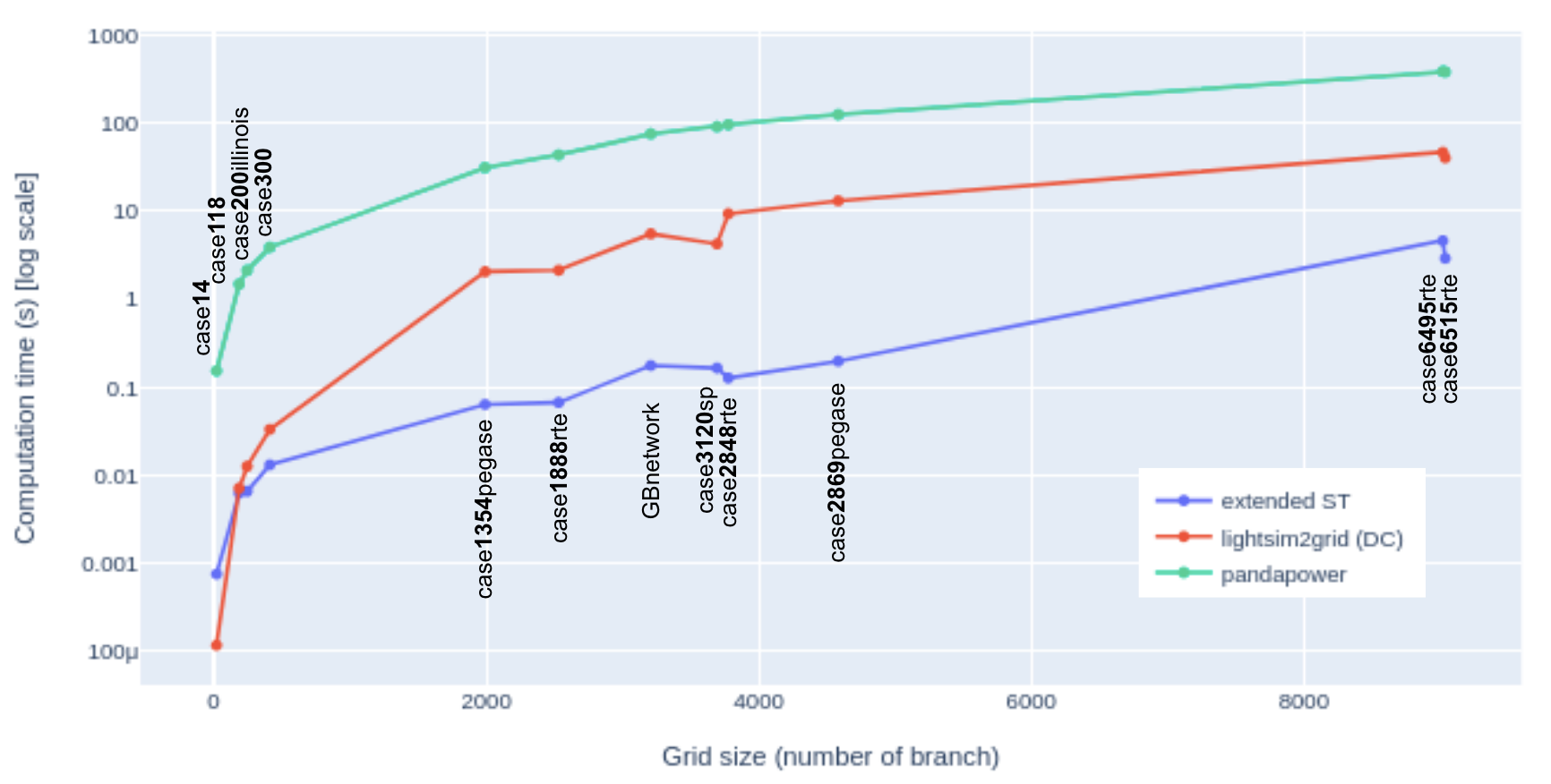
Figure 3: Comparing security analysis computation time in second (s) across grid sizes for extended ST and 2 reference DC power flow solvers LightSim2Grid [13], PandaPower [14].

The computation time for security analysis can be improved through parallelization. This is achievable due to the independence of equation systems that need to be solved for each line outage simulation. Additionally, the interpretability of $\beta$ parameters allows for further enhancements in the computation time of security analysis. Topological actions locally change the power flow distribution. If full grid topology information is available, a straightforward heuristic can leverage this aspect by commencing the computation of security analysis for the nearest electrical lines where the topological action was applied and subsequently ending the computation when all $\beta$ values equal 1. One can then reduce the range of resimulating outage lines to consider when a topological action is applied. We could expect to probably reduce the refresh of security analysis to about 50 contingencies in general, and not the entire grid. On the IEEE 118 grid, this could account for an increased speed-up of a factor 3 for instance, by leveraging all aspect of extended ST. This here ends our short tour of first application examples of extended ST.

IV Conclusion

In this paper, we have demonstrated the existence and unicity of an extended superposition theorem for all type of unitary topological changes and their mixture. We have seen the speed-up and interpretability it can bring to power flow computations and their analysis. In particular applications for remedial action and security analysis can alrready benefit for it. We believe it can be of very generic use and a foundation for improvements in many applications as well as integrated in optimization formulations such as in optimal power flow. Future work will aim at revisiting some recent applications that involves topological changes in light of extended ST, such as grid segmentation [15, 16], leap net proxy power flow [17] or topological expert system [18] . It could result in better interpretation of choices or results, and possibly help improving the respective implementations.

References

• [1] R. L. Boylestad and L. Nashelsky, Electronic devices and circuit theory. Pearson Education India, 2009.
• [2] A. Marot, A. Kelly, M. Naglic, V. Barbesant, J. Cremer, A. Stefanov, and J. Viebahn, “Perspectives on future power system control centers for energy transition,” Journal of Modern Power Systems and Clean Energy, vol. 10, no. 2, pp. 328–344, 2022.
• [3] A. Marot, B. Donnot, C. Romero, B. Donon, M. Lerousseau, L. Veyrin-Forrer, and I. Guyon, “Learning to run a power network challenge for training topology controllers,” Electric Power Systems Research, vol. 189, p. 106635, 2020.
• [4] M. Shahidehpour, H. Yamin, and Z. Li, Market operations in electric power systems: forecasting, scheduling, and risk management. John Wiley & Sons, 2003.
• [5] A. J. Wood, B. F. Wollenberg, and G. B. Sheblé, Power generation, operation, and control. John Wiley & Sons, 2013.
• [6] K. Bhattacharya, M. H. Bollen, and J. E. Daalder, Operation of restructured power systems. Springer Science & Business Media, 2012.
• [7] T. Guler, G. Gross, and M. Liu, “Generalized line outage distribution factors,” IEEE Transactions on Power systems, vol. 22, no. 2, pp. 879–881, 2007.
• [8] J. van Dijk, J. Viebahn, B. Cijsouw, and J. van Casteren, “Bus split distribution factors,” 2023.
• [9] B. Stott, J. Jardim, and O. Alsaç, “Dc power flow revisited,” IEEE Transactions on Power Systems, vol. 24, no. 3, pp. 1290–1300, 2009.
• [10] P. A. Ruiz, E. Goldis, A. M. Rudkevich, M. C. Caramanis, C. R. Philbrick, and J. M. Foster, “Security-constrained transmission topology control milp formulation using sensitivity factors,” IEEE Transactions on Power Systems, vol. 32, no. 2, pp. 1597–1605, 2016.
• [11] E. A. Goldis, P. A. Ruiz, M. C. Caramanis, X. Li, C. R. Philbrick, and A. M. Rudkevich, “Shift factor-based scopf topology control mip formulations with substation configurations,” IEEE Transactions on Power Systems, vol. 32, no. 2, pp. 1179–1190, 2016.
• [12] B. Donnot, “Grid2op- A testbed platform to model sequential decision making in power systems. .” \urlhttps://GitHub.com/rte-france/grid2op, 2020.
• [13] B. Donnot, “Lightsim2grid - A c++ backend targeting the Grid2Op platform. .” \urlhttps://GitHub.com/bdonnot/lightsim2grid, 2020.
• [14] L. Thurner, A. Scheidler, F. Schäfer, J.-H. Menke, J. Dollichon, F. Meier, S. Meinecke, and M. Braun, “pandapower—an open-source python tool for convenient modeling, analysis, and optimization of electric power systems,” IEEE Transactions on Power Systems, vol. 33, no. 6, pp. 6510–6521, 2018.
• [15] A. Marot, S. Tazi, B. Donnot, and P. Panciatici, “Guided machine learning for power grid segmentation,” in 2018 IEEE PES Innovative Smart Grid Technologies Conference Europe (ISGT-Europe), pp. 1–6, 2018.
• [16] N. Henka, Q. Francois, S. Tazi, M. Ruiz, and P. Panciatici, “Power grid segmentation for local topological controllers,” Electric Power Systems Research, vol. 213, p. 108302, 2022.
• [17] B. Donon, B. Donnot, I. Guyon, Z. Liu, A. Marot, P. Panciatici, and M. Schoenauer, “Leap nets for system identification and application to power systems,” Neurocomputing, vol. 416, pp. 316–327, 2020.
• [18] A. Marot, B. Donnot, S. Tazi, and P. Panciatici, “Expert system for topological remedial action discovery in smart grids,” 2018.