Resummed spinning waveforms from five-point amplitudes

Abstract

We compute the classical tree-level five-point amplitude for the two-to-two scattering of spinning celestial objects with the emission of a graviton. Using this five-point amplitude, we then turn to the computation of the leading-order time-domain gravitational waveform. The method we describe is suitable for arbitrary values of classical spin of Kerr black holes and does not require any expansion in powers of the spin. In this paper we illustrate it in the simpler case of the scattering of one Kerr and one Schwarzschild black hole. An important ingredient of our calculation is a novel form of the Compton amplitude with spinning particles including contact terms derived from matching to black-hole perturbation theory calculations. This ensures that our waveform is valid up to at least fourth order in the spin. Our method can be applied immediately to generate improved waveforms once higher-order contact terms in the Compton amplitude become available. Finally, we show the formula for the gravitational memory to all orders in the spin, which is in agreement with our results.

1 Introduction

Since the first direct observation of gravitational waves [1, 2, 3, 4, 5], a flurry of observations and theoretical predictions have greatly advanced the fields of black-hole physics and general relativity. Important questions regarding the intrinsic properties of black holes, the dynamics of binary black-hole processes, and more, can all be investigated in depth through high-precision gravitational-wave observations and theoretical calculations.

One widely used and highly successful analytical tool for the study of binary black-hole systems is the Post-Newtonian (PN) expansion [6, 7, 8, 9, 10, 11, 12, 13, 14, 15, 16, 17, 18, 19, 20, 21, 22, 23, 24, 25, 26, 27, 28, 29, 30, 31, 32, 33, 34, 35, 36, 37, 38, 39] and the effective one-body formulation [40, 41, 42, 43, 44, 45]. Recently, several varieties of modern methods, e.g. the double copy [46, 47, 48, 49, 50, 51, 52, 53], the Kosower-Maybee-O’Connell (KMOC) formalism [54], heavy-mass effective theories [55, 56, 57, 58, 59, 60, 61, 62], the eikonal approach [63, 64, 65, 66], velocity cuts and the exponential representation of the $S$-matrix [67, 68, 69], worldline effective theory [70, 71, 72, 73, 74, 75] and worldline quantum field theory [76, 77, 78], have emerged as powerful theoretical frameworks for studying binary black-hole physics to high Post-Minkowskian (PM) order from different points of view. In particular they have been successfully applied to compute the conservative part of the binary dynamics of gravitationally interacting systems [79, 80, 81, 82, 83, 84, 85, 86, 87, 88, 67, 89, 90, 91, 92, 93, 94, 95, 96, 97, 98, 99, 100, 69, 101, 102, 103, 104, 105, 106, 107] to high orders in the PM expansion.

Research directly focused on the gravitational waveforms of binary black-hole systems in the PM expansion is evolving rapidly. The tree-level waveforms for spinless objects were computed in [108, 109, 110] and reproduced in [77, 111] in the worldline picture. The tree-level waveform was studied in [112, 113] using the scattering-amplitude based KMOC formalism [54, 112] and investigated using the eikonal approach in [64, 63]. At one loop, the study of the gravitational waveform was initiated recently in [62, 114, 115, 116] where the principal value contribution was obtained and shown to be consistent between KMOC and a heavy-mass effective field theory (HEFT) framework. The remaining terms beyond this principal value part were pointed out in [117] and shown to give an additional contribution to the waveform. The existence of such terms was also suggested by comparing with the Multipolar-Post-Minkowskian waveform in [118].

Gravitational waveforms are influenced by various intrinsic properties of black holes. One of the most significant factors among them is their spin. An important building block for including spin effects in waveforms is the minimal coupling between a classical spinning black hole and a graviton obtained using the massive spinor-helicity formalism [119]. Further important developments made use of spinor helicity [120, 121, 122, 123, 124, 125, 56, 126, 127, 128, 129, 130, 131, 132, 133, 134, 135], the covariant amplitude form  [136, 137, 138, 55, 139, 43, 44, 140, 141, 142, 143], gravitational solutions [144, 145, 146, 147, 148], and the worldline picture [106, 149, 76, 77, 103, 150]. At tree level, the spin contribution to the waveform up to quadratic order was obtained in [151, 152] using a worldline effective theory.

In this paper, by employing the definition of waveforms in terms of five-point amplitudes [112], we compute gravitational waveforms involving spinning black holes, crucially without the need to expand in their spin. The building blocks entering the recursive BCFW construction [153, 154] of the five-point amplitude, adapted to the classical amplitude [62], are the three-point and four-point Compton amplitudes with massive particles of arbitrary classical spin, which were constructed in [155, 156] using a bootstrap technique which makes use of entire functions. After expanding in spin, this form of the Compton amplitude agrees with results obtained from black-hole perturbation theory [145, 142, 134] for Kerr black holes up to at least fourth order in spin. However we note that this Compton amplitude can be upgraded with additional contact terms to match with the Teukolsky equation [144, 145], and the method discussed in this paper can be immediately applied to incorporate such additional terms once these are available.

In this work we mainly focus on the time-domain waveform. First, we perform the Fourier transform over the frequency; the exponential factors in the spinning amplitude then produce a simple extra delta function when transforming to impact parameter space [151, 77, 114]. This additional delta function localises the integral further and simplifies the tree-level amplitude greatly. Finally, thanks to Cauchy’s theorem, as used in [157], the remaining one-dimensional integral localises to contour integrals around physical poles only. We stress here that our approach does not require any expansion in the spin parameters. Importantly, this allows us to preserve the (partially) resummed form of the Compton amplitude, and thus enables us to obtain a first glimpse at large-spin effects in gravitational waveforms.

The rest of the paper is organised as follows. In the next section we introduce the kinematics of the process, together with the definition of the spin variables we employ. In Section 3 we introduce the three-point amplitude and the Compton amplitude with spinning particles. These are then used in Section 4 to construct the five-point amplitude of four massive spinning particles with the emission of a gravitational wave, using a particular form of the BCFW recursion relation introduced in [62] for classical amplitudes. In Section 5 we introduce the general method to compute the time-domain waveforms and illustrate how this computation reduces to a sum of residues on physical factorisation poles only, in the simpler case of spinless particles. We then present the general expression of the waveform for arbitrary spins of the two black holes. In Section 6 we specialise to the case of a Schwarzschild and a Kerr black hole, and also present several plots of the waveforms for increasing values of the spin of the Kerr black hole. In Section 7 we make some interesting observations by comparing the waveforms obtained using the resummed Compton amplitudes to those derived from the Compton amplitudes expanded in the spin parameter. Section 8 presents a short derivation of the memory of the gravitational wave in the spinning case, to all orders in the spins of the Kerr black holes, which we have then used to test our analytic results. Finally, two appendices complete the paper. In Appendix A we perform some useful simplifications of the expression of the four-point Compton amplitude, which are convenient in the derivation of the memory; and in Appendix B we list the coefficients appearing in the $q_{1}^{2}$- and $q_{2}^{2}$-channels of the classical, tree-level five-point amplitude derived in Section 5.

The interested reader can find Mathematica notebooks with expressions for the spinning HEFT amplitudes with one emitted graviton, and explicit time-domain waveform results in the system of a Schwarzschild and a Kerr black hole SpinningWaveform GitHub repository.

Note added: While preparing this manuscript we became aware of the nice work [157], with which our paper has some overlap. We have checked that our results agree with theirs.

2 Kinematics of the scattering and spin variables

Here we review the kinematics of the scattering of two heavy spinning particles of masses $m_{1}$ and $m_{2}$ and spin vectors $a_{1}$ and $a_{2}$, with the emission of a graviton of momentum $k$:

$$\begin{array}[]{lr}\leavevmode\hbox to176.37pt{\vbox to109.36pt{\text{[drawing]}}}&\end{array} p_{1}=\bar{p}_{1}+\dfrac{q_{1}}{2} p_{2}=\bar{p}_{2}+\dfrac{q_{2}}{2} p_{2}^{\prime}=\bar{p}_{2}-\dfrac{q_{2}}{2} \ \ p_{1}^{\prime}=\bar{p}_{1}-\dfrac{q_{1}}{2} k=q_{1}+q_{2} p_{1}=\bar{p}_{1}+\dfrac{q_{1}}{2} p_{2}=\bar{p}_{2}+\dfrac{q_{2}}{2} p_{2}^{\prime}=\bar{p}_{2}-\dfrac{q_{2}}{2} \ \ p_{1}^{\prime}=\bar{p}_{1}-\dfrac{q_{1}}{2} k=q_{1}+q_{2}$$ (2.1)

As usual we have introduced barred variables, defined as [158, 87]

$$\begin{split}p_{1}&=\bar{p}_{1}+\frac{q_{1}}{2}\,,\qquad p_{1}^{\prime}=\bar{p}_{1}-\frac{q_{1}}{2}\,,\\ p_{2}&=\bar{p}_{2}+\frac{q_{2}}{2}\,,\qquad p_{2}^{\prime}=\bar{p}_{2}-\frac{q_{2}}{2}\,,\end{split}$$ (2.2)

which satisfy

$$\bar{p}_{1}{\cdot}q_{1}=\bar{p}_{2}{\cdot}q_{2}=0\,.$$ (2.3)

We also introduce barred masses,

$$\bar{m}_{i}^{2}\coloneqq\bar{p}_{i}^{2}=m_{i}^{2}-\frac{q_{i}^{2}}{4}\,,\qquad i=1,2\,,$$ (2.4)

with the HEFT expansion being organised in powers of the $\bar{m}_{i}$.

To parameterise the scattering process we choose five independent Lorentz-invariant quantities as in [62],

$$\begin{split}y\coloneqq v_{1}{\cdot}v_{2}\geq 1\ ,\qquad q_{i}^{2}\leq 0\ ,\qquad w_{i}\coloneqq v_{i}{\cdot}k\geq 0\,,\qquad i=1,2,\end{split}$$ (2.5)

where the four-velocities are defined by $p_{i}{=}m_{i}v_{i}$, with $v_{i}^{2}{=}1$. We also note that $y$ is the relativistic factor $\frac{1}{\sqrt{1-v_{\rm rel}^{2}}}$, where $v_{\rm rel}$ is the relative velocity of one of the two heavy particles in the rest frame of the other. We will also use the barred versions $\bar{w}_{i}\coloneqq\bar{v}_{i}{\cdot}k$ and $\bar{y}\coloneqq\bar{v}_{1}{\cdot}\bar{v}_{2}$ of the above quantities, with $\bar{p}_{i}\coloneqq\bar{m}_{i}\bar{v}_{i}$ and $\bar{v_{i}}^{2}=1$.

The spin tensors for incoming and outgoing massive particles in terms of the spin vectors $s_{i}$ are given by

$$\begin{split}&S_{i}^{\mu\nu}(p_{i})=-\frac{1}{m_{i}}\epsilon^{\mu\nu\alpha\beta}p_{i\,\alpha}s_{i\,\beta}(p_{i})\,,\qquad S_{i}^{\mu\nu}(p_{i}^{\prime})=-\frac{1}{m_{i}}\epsilon^{\mu\nu\alpha\beta}p^{\prime}_{i\,\alpha}s_{i\,\beta}(p_{i}^{\prime})\,.\end{split}$$ (2.6)

To expand this in the heavy-mass limit we change variables from $p_{i},p_{i}^{\prime}$ to $\bar{p}_{i}$ and $q_{i}$ as in (2.2). We follow the method of [125] and use an infinitesimal Lorentz transformation from $\bar{p}_{i}$ to $\bar{p}_{i}\pm\dfrac{q}{2}$ to write

$$s_{i}^{\mu}\big{(}\bar{p}_{i}\pm\frac{q}{2}\big{)} =(\delta_{\nu}^{\mu}\pm{\omega^{\mu}}_{\nu})s_{i}(\bar{p}_{i})^{\nu}$$

$$=\Big{[}\delta_{\nu}^{\mu}\mp\frac{1}{2\bar{m}^{2}}(\bar{p}_{i}^{\mu}q_{\nu}-q^{\mu}\bar{p}_{i\,\nu})\Big{]}s_{i}(\bar{p}_{i})^{\nu}$$ (2.7)

$$=s_{i}(\bar{p}_{i})^{\mu}\mp\frac{\bar{p}_{i}^{\mu}}{2\bar{m}^{2}}q{\cdot}s_{i}(\bar{p}_{i})+\mathcal{O}(\bar{m}^{-2})\,.$$

This is valid since $\bar{m}_{i}$ (which will eventually be the classical mass) is much larger than the typical value of $q$. This allows us to expand the spin tensors as

$$\begin{split}S_{i}^{\mu\nu}(p_{i})&=-\frac{1}{\bar{m}_{i}}\epsilon^{\mu\nu\alpha\beta}\bar{p}_{i\,\alpha}s_{i\,\beta}(\bar{p})-\frac{1}{2\bar{m}_{i}}\epsilon^{\mu\nu\alpha\beta}q_{\alpha}s_{i\,\beta}(\bar{p}_{i})+\mathcal{O}(\bar{m}^{-2})\,,\\ S_{i}^{\mu\nu}(p^{\prime}_{i})&=-\frac{1}{\bar{m}_{i}}\epsilon^{\mu\nu\alpha\beta}\bar{p}_{i\,\alpha}s_{i\,\beta}(\bar{p}_{i})+\frac{1}{2\bar{m}_{i}}\epsilon^{\mu\nu\alpha\beta}q_{\alpha}s_{i\,\beta}(\bar{p}_{i})+\mathcal{O}(\bar{m}^{-2})\,,\end{split}$$ (2.8)

where, remarkably, the shifts in $s_{i}^{\mu}(p_{i}^{(\prime)})$ drop out to this order in the $\bar{m}$ expansion, due to the antisymmetry of the Levi-Civita. We can also define the classical spin parameter as

$$a_{i}^{\mu}\coloneqq\frac{s_{i}^{\mu}(\bar{p}_{i})}{\bar{m}_{i}}\,,$$ (2.9)

to write

$$\begin{split}S_{i}^{\mu\nu}(p_{i})&=-\epsilon^{\mu\nu\alpha\beta}\Big{(}\bar{p}_{i\,\alpha}+\frac{q_{\alpha}}{2}\Big{)}a_{i\,\beta}+\mathcal{O}(\bar{m}_{i}^{-2})\,,\\ S_{i}^{\mu\nu}(p_{i}^{\prime})&=-\epsilon^{\mu\nu\alpha\beta}\Big{(}\bar{p}_{i\,\alpha}-\frac{q_{\alpha}}{2}\Big{)}a_{i\,\beta}+\mathcal{O}(\bar{m}_{i}^{-2})\,.\end{split}$$ (2.10)

Finally, in the large $\bar{m}_{i}$ limit the two spin tensors in (2.10) become the same, and we define our classical spin tensors as

$$S_{i}^{\mu\nu}\coloneqq-\epsilon^{\mu\nu\rho\sigma}\bar{p}_{i\,\rho}a_{i\,\sigma}\,,$$ (2.11)

which satisfies $S^{\mu\nu}_{i}\bar{p}_{i\nu}{=}0$, known as the spin supplementary condition [159, 33], while $a_{i}$ satisfies $\bar{p}_{i}{\cdot}a_{i}=0$. We can also invert this relation,

$$a^{\mu}_{i}=-\frac{1}{2\bar{m}^{2}_{i}}\epsilon^{\mu\nu\alpha\beta}\bar{p}_{i\,\nu}S_{i\,\alpha\beta}\,.$$ (2.12)

Note that $a^{\mu}_{i}$ has mass dimension $-1$ so that $S^{\mu\nu}_{i}$ is dimensionless. The spin vector of a heavy particle is then

$$s^{\mu}_{i}\coloneqq\bar{m}_{i}a^{\mu}_{i}\,.$$ (2.13)

Much like $\bar{p}^{\mu}$ and $\bar{v}^{\mu}$, both $s^{\mu}$ and $a^{\mu}$ are well defined in the classical/large-$m$ limit. Finally, the gravitational coupling we use is $\kappa\coloneqq\sqrt{32\pi G}$.

3 Classical gravitational Compton amplitude with spin

3.1 Three-point amplitude

The three-point amplitude for two classical massive spinning particles is given by [119, 121, 122, 128]

$$\mathcal{M}_{3}=-i\kappa\,(\bar{p}{\cdot}\varepsilon_{1})^{2}\exp\left(-i\frac{k_{1}{\cdot}S\cdot\varepsilon_{1}}{\bar{p}{\cdot}\varepsilon_{1}}\right)\,,$$ (3.1)

where $p$ is the momentum of the massive particle, $k_{1}$ is the momentum of the graviton with polarisation $\varepsilon_{1}$ and $S$ is the spin tensor of the massive particle introduced in (2.11). The amplitude (3.1) can also be written as [139, 160, 155]

$$\mathcal{M}_{3}=-i\kappa(\bar{p}{\cdot}\varepsilon_{1})({\mathsf{w}}_{1}{\cdot}\varepsilon_{1})\,,$$ (3.2)

where

$$\begin{split}{\mathsf{w}}_{1}^{\mu}&\coloneqq\cosh(k_{1}{\cdot}a)\bar{p}^{\mu}-i\frac{\sinh(k_{1}{\cdot}a)}{k_{1}{\cdot}a}(k_{1}{\cdot}S)^{\mu}\,,\end{split}$$ (3.3)

and we have used the notation $(k_{1}{\cdot}S)^{\mu}=k_{1\nu}S^{\nu\mu}$.

3.2 The Compton amplitude

We now move on to discuss the four-point amplitude. For convenience, in this section we will call the momenta $p,k_{1},k_{2},p^{\prime}$ where $p,p^{\prime}$ are the momenta of the massive particles, $p^{2}{=}(p^{\prime})^{2}{=}m^{2}$ and $k_{1,2}$ are the momenta of the gravitons, with $k_{1,2}^{2}{=}0$.

(3.4)

The four-point classical Compton amplitude can be divided into three pieces [156],

$$\mathcal{M}_{4}=\frac{-i\mathcal{N}_{\rm dc}}{2k_{1}{\cdot}k_{2}}+\frac{-i\mathcal{N}_{\rm r}}{4\bar{p}{\cdot}k_{1}\bar{p}{\cdot}k_{2}}-i\mathcal{N}_{\rm c}.$$ (3.5)

The first term is obtained from the double copy and corresponds to propagation without changing the direction or magnitude of the spin [155],

$$\mathcal{N}_{\rm dc} =-\Bigg{[}\frac{{\mathsf{w}}_{1}{\cdot}F_{1}{\cdot}F_{2}{\cdot}{\mathsf{w}}_{2}}{k_{1}{\cdot}\bar{p}}-\Big{(}iG_{2}\left(x_{1},x_{2}\right)(a{\cdot}F_{1}{\cdot}F_{2}{\cdot}S{\cdot}k_{2}+a{\cdot}F_{2}{\cdot}F_{1}{\cdot}S{\cdot}k_{1})$$

$$+iG_{1}\left(x_{12}\right)\text{tr}\left(F_{1}{\cdot}S{\cdot}F_{2}\right)+G_{1}(x_{1})G_{1}(x_{2})(a{\cdot}F_{1}{\cdot}\bar{p}a{\cdot}F_{2}{\cdot}k_{1}-a{\cdot}F_{1}{\cdot}k_{2}a{\cdot}F_{2}{\cdot}\bar{p})$$

$$+k_{1}{\cdot}\bar{p}\,G_{1}(x_{1})G_{1}(x_{2})a{\cdot}F_{1}{\cdot}F_{2}{\cdot}a\Big{)}\Bigg{]}\Big{(}\frac{\bar{p}{\cdot}F_{1}{\cdot}F_{2}{\cdot}\bar{p}}{k_{2}{\cdot}\bar{p}}\Big{)}\,,$$ (3.6)

with

$$x_{i}\coloneqq k_{i}{\cdot}a\,,\quad x_{i\ldots j}\coloneqq(k_{i}+\cdots+k_{j}){\cdot}a\ ,\quad F^{\mu\nu}_{i}=k_{i}^{\mu}\varepsilon_{i}^{\nu}-\varepsilon_{i}^{\mu}k_{i}^{\nu}\,.$$ (3.7)

Note that it contains both massless and massive poles and we already take the HEFT expansion. This term gives the minimal amplitude to fit the test particle scattering angle in the Kerr metric.

The second term allows for a change of direction of the spin, and we refer to it as the “spin-flip” term [156],

$$\mathcal{N}_{\rm r} =\Big{[}(\partial_{x_{1}}-\partial_{x_{2}})G_{1}(x_{1})G_{1}(x_{2})\Big{]}$$

$$\times\Big{[}\bar{p}{\cdot}k_{2}\ (\bar{p}^{2}a{\cdot}F_{1}{\cdot}F_{2}{\cdot}a\ a{\cdot}F_{2}{\cdot}F_{1}{\cdot}\bar{p}+a^{2}\bar{p}{\cdot}F_{1}{\cdot}F_{2}{\cdot}\bar{p}\ a{\cdot}F_{1}{\cdot}F_{2}{\cdot}\bar{p})-(1\leftrightarrow 2)\Big{]}$$

$$+i\Big{[}(\partial_{x_{1}}-\partial_{x_{2}})G_{2}(x_{1},x_{2})\Big{]}$$

$$\times\Big{[}\bar{p}{\cdot}k_{2}\ a{\cdot}F_{2}{\cdot}F_{1}{\cdot}\bar{p}\ (a{\cdot}F_{2}{\cdot}\bar{p}\ a{\cdot}\widetilde{F}_{1}{\cdot}\bar{p}-a{\cdot}F_{1}{\cdot}\bar{p}\ a{\cdot}\widetilde{F}_{2}{\cdot}\bar{p})+(1\leftrightarrow 2)\Big{]}\,,$$ (3.8)

where $\widetilde{F}^{\mu\nu}\equiv\frac{1}{2}\epsilon^{\mu\nu\rho\sigma}F_{\rho\sigma}$ denotes the Hodge dual of the linearised field strength. Note that this term only gives rise to massive poles. Finally, the last contribution consists of contact terms,

$$\mathcal{N}_{c} =\Big{[}{(\partial_{x_{1}}-\partial_{x_{2}})^{2}\over 2!}{G_{1}(x_{1})}{G_{1}(x_{2})}\Big{]}\Big{[}a{\cdot}F_{1}{\cdot}\bar{p}\ a{\cdot}F_{2}{\cdot}\bar{p}\ a{\cdot}F_{1}{\cdot}F_{2}{\cdot}a$$ (3.9)

$$-{1\over 2}a^{2}(a{\cdot}F_{1}{\cdot}F_{2}{\cdot}\bar{p}\ a{\cdot}F_{2}{\cdot}F_{1}{\cdot}\bar{p}-a{\cdot}F_{1}{\cdot}F_{2}{\cdot}a\ \bar{p}{\cdot}F_{1}{\cdot}F_{2}{\cdot}\bar{p})\Big{]}$$

$$+e_{1}\Big{[}{i(\partial_{x_{1}}-\partial_{x_{2}})^{2}\over 2!}{G_{2}(x_{1},x_{2})}\Big{]}\Big{[}a{\cdot}F_{1}{\cdot}F_{2}{\cdot}a\ a{\cdot}F_{2}{\cdot}\bar{p}\ a{\cdot}\widetilde{F}_{1}{\cdot}\bar{p}-(1\leftrightarrow 2)\Big{]}$$

$$+e_{2}\Big{[}{i(\partial_{x_{1}}-\partial_{x_{2}})^{2}\over 2!}{G_{2}(x_{1},x_{2})}\Big{]}\Big{[}\bar{p}^{2}(a{\cdot}F_{1}{\cdot}F_{2}{\cdot}a)(a{\cdot}F_{2}{\cdot}\widetilde{F}_{1}{\cdot}a)-(1\leftrightarrow 2)\Big{]}\,$$

$$+e_{3}\Big{[}{i(\partial_{x_{1}}-\partial_{x_{2}})^{2}\over 2!}{G_{2}(x_{1},x_{2})}\Big{]}\Big{[}a^{2}(a{\cdot}F_{2}{\cdot}F_{1}{\cdot}\bar{p})(a{\cdot}\widetilde{F}_{1}{\cdot}F_{2}{\cdot}\bar{p})-(1\leftrightarrow 2)\Big{]}\,.$$

The $G$-functions appearing in the expressions above can be defined in terms of hyperbolic functions as [155]

$$G_{1}(x) :=\frac{\sinh(x)}{x}\,,$$

$$G_{2}(x_{1},x_{2}) :={1\over x_{2}}\Big{(}{\sinh(x_{{12}})\over{x_{12}}}-\cosh(x_{2})\,{\sinh(x_{1})\over{x_{1}}}\Big{)},$$ (3.10)

and are entire functions, free of singularities. Note that $G_{2}(x_{2},x_{1})=-G_{2}(x_{1},x_{2})$.

The contact terms in the first two lines of (3.9) only begin contributing at quartic order in the spin and their numerical coefficients have been fixed against results at quartic order in the spin arising from black-hole perturbation theory (BHPT) [145] or equivalently using the “spin-shift symmetry” [142, 134]. At $\mathcal{O}(a^{4})$, these two methods to constrain the contact terms are in agreement.

The remaining three lines in (3.9) involve contact terms which contribute from quintic order in the spin. We have chosen to fix their numerical coefficients $e_{1},e_{2},e_{3}$ assuming spin-shift symmetry applied at this order [133, 142], setting them to be $e_{1}{=}-3/4,\,e_{2}{=}0,\,e_{3}{=}0$. However, we note that recent work [145] has shown that at $\mathcal{O}(a^{5})$ the spin-shift symmetry is in fact broken, and instead such coefficients should be fixed by comparison to BHPT or alternatively fixed to the method of multipole moments of the Kerr BH [161]. These two methods are in agreement at $\mathcal{O}(a^{5})$ [161] but do not agree with spin-shift symmetry. Therefore, the results derived here are only applicable to Kerr black holes up to quartic order in the spin. We have chosen to set $e_{1}{=}-3/4,\,e_{2}{=}0,\,e_{3}{=}0$ simply to illustrate the general matching principle, although our method makes it easy to deal with any values of the $e_{i}$’s and also with further contact terms starting at $\mathcal{O}(a^{6})$ and beyond, as we will discuss in [162].

Finally, we note here that, as described in detail in [144, 145], results from BHPT are valid in the physical regime $\frac{a_{i}}{Gm_{i}}<1$ but can be analytically continued to the super-extremal regime where $\frac{a_{i}}{Gm_{i}}>1$ in order to match with results formulated from amplitudes. Such an analytic continuation is in fact trivial up to $\mathcal{O}(a^{4})$. We conclude that at leading PM order and up to fourth order in spin the Compton amplitude, and hence our spin-expanded results for the waveform, do not distinguish between physical versus super-extremal Kerr.

4 Spinning five-point amplitude

The crucial ingredient to compute the waveforms is the classical part of the five-point amplitude of two spinning particles with one radiated graviton. It can be derived using the HEFT BCFW recursion relation introduced in [62] and is obtained from the following two recursive diagrams,

(4.1)

corresponding to the $q_{1}^{2}$ and $q_{2}^{2}$ channels, respectively. In the scalar case, these BCFW diagrams capture all of the ‘contact terms’ in the classical amplitude (that is terms without poles in $q_{1}^{2}$ or $q_{2}^{2}$ but possibly with massive poles). In the spinning case we will follow the same procedure and, although we have no general proof that these contact terms are captured fully, we have checked that the contributions from the two BCFW diagrams satisfy the correct soft behaviour. Regardless, such contact terms without poles in $q_{1}^{2}$ or $q_{2}^{2}$ do not contribute to the tree-level waveform as we will see in Sections 5 and 7.

The contribution of each of the two diagrams is obtained by gluing a three-point amplitude with a four-point Compton amplitude, given in (3.1) and (3.5), respectively. In doing so one has to sum over the intermediate states of the exchanged graviton, using

$$\sum_{h}\varepsilon^{\mu_{a}}_{-\hat{q}}{\varepsilon}^{\nu_{a}}_{-\hat{q}}{\varepsilon}^{\mu_{b}}_{\hat{q}}\varepsilon^{\nu_{b}}_{\hat{q}}=\frac{1}{2}\Big{[}\eta^{\mu_{a}\mu_{b}}\eta^{\nu_{a}\nu_{b}}+\eta^{\mu_{a}\nu_{b}}\eta^{\nu_{a}\mu_{b}}-\frac{2}{D-2}\eta^{\mu_{a}\nu_{a}}\eta^{\mu_{b}\nu_{b}}\Big{]}\,.$$ (4.2)

For convenience, we introduce a tensor current by extracting the polarisation vector from the Compton amplitude:

$$\mathcal{J}^{\mu\nu}_{i}\varepsilon_{\mu\nu}=\mathcal{M}_{4}(-q_{i},k,\bar{v}_{i},a_{i})\,.$$ (4.3)

Then, the amplitude in each channel is of the form

$$\begin{split}\mathcal{M}_{q_{1}^{2}}&={1\over q_{1}^{2}}\sum_{h}\Big{(}\cosh(a_{1}{\cdot}q_{1})(\bar{v}_{1}{\cdot}\varepsilon)^{2}\varepsilon_{\mu\nu}\mathcal{J}^{\mu\nu}_{1}-iG(a_{1}{\cdot}q_{1})\bar{v}_{1}{\cdot}\varepsilon\,q_{1}{\cdot}S_{1}{\cdot}\varepsilon\,\varepsilon_{\mu\nu}\mathcal{J}^{\mu\nu}_{1}\Big{)}\\ &={1\over q_{1}^{2}}\Big{(}\cosh(a_{1}{\cdot}q_{1})\big{(}\bar{v}_{1}{\cdot}\mathcal{J}_{1}{\cdot}\bar{v}_{1}-{1\over 2}\text{tr}(\mathcal{J}_{1})\big{)}-{i\over 2}G(a_{1}{\cdot}q_{1})\big{(}q_{1}{\cdot}S_{1}{\cdot}\mathcal{J}_{1}{\cdot}\bar{v}_{1}-\bar{v}_{1}{\cdot}\mathcal{J}_{1}{\cdot}S_{1}{\cdot}q_{1}\big{)}\Big{)}\,,\end{split}$$ (4.4)

and

$$\begin{split}\mathcal{M}_{q_{2}^{2}}&={1\over q_{2}^{2}}\sum_{h}\Big{(}\cosh(a_{2}{\cdot}q_{2})(\bar{v}_{2}{\cdot}\varepsilon)^{2}\varepsilon_{\mu\nu}\mathcal{J}^{\mu\nu}_{2}-iG(a_{2}{\cdot}q_{2})\bar{v}_{2}{\cdot}\varepsilon\,q_{2}{\cdot}S_{2}{\cdot}\varepsilon\,\varepsilon_{\mu\nu}\mathcal{J}^{\mu\nu}_{2}\Big{)}\\ &={1\over q_{2}^{2}}\Big{(}\cosh(a_{2}{\cdot}q_{2})\big{(}\bar{v}_{2}{\cdot}\mathcal{J}_{2}{\cdot}\bar{v}_{2}-{1\over 2}\text{tr}(\mathcal{J}_{2})\big{)}-{i\over 2}G(a_{2}{\cdot}q_{2})\big{(}q_{2}{\cdot}S_{2}{\cdot}\mathcal{J}_{2}{\cdot}\bar{v}_{2}-\bar{v}_{2}{\cdot}\mathcal{J}_{2}{\cdot}S_{2}{\cdot}q_{2}\big{)}\Big{)}\,.\end{split}$$ (4.5)

The full amplitude can be obtained directly adding (4.4) and (4.5),

$$\mathcal{M}_{5,\rm HEFT}=\mathcal{M}_{q_{1}^{2}}+\mathcal{M}_{q_{2}^{2}}\,.$$ (4.6)

Both channels have the spurious pole $1\over k{\cdot}q_{1}$, which cancels after summing the two contributions. To see this, we must use the Bianchi identity in $D$-dimensional momentum space [163]

$$\begin{split}A{\cdot}F_{k}{\cdot}B\ k{\cdot}C+B{\cdot}F_{k}{\cdot}C\ A{\cdot}k+C{\cdot}F_{k}{\cdot}A\ k{\cdot}&B=0\,,\end{split}$$ (4.7)

where $A,B,C$ can be any vector. For example, a particular application is

$$\bar{v}_{1}{\cdot}S_{2}{\cdot}F_{k}{\cdot}q_{2}=\frac{k{\cdot}q_{2}\bar{v}_{1}{\cdot}F_{k}{\cdot}S_{2}{\cdot}\bar{v}_{1}-k{\cdot}S_{2}{\cdot}\bar{v}_{1}\bar{v}_{1}{\cdot}F_{k}{\cdot}q_{2}}{q_{2}{\cdot}\bar{v}_{1}}.$$ (4.8)

The resulting expression for the amplitude only contains the following field-strength products:

$$a_{1}{\cdot}F_{k}{\cdot}\bar{v}_{1}, a_{2}{\cdot}F_{k}{\cdot}\bar{v}_{1}, q_{1}{\cdot}F_{k}{\cdot}\bar{v}_{1}, v_{1}{\cdot}F_{k}{\cdot}\bar{v}_{2}, q_{1}{\cdot}S_{1}{\cdot}F_{k}{\cdot}\bar{v}_{1},$$

$$q_{1}{\cdot}S_{2}{\cdot}F_{k}{\cdot}\bar{v}_{1}, v_{1}{\cdot}F_{k}{\cdot}S_{1}{\cdot}\bar{v}_{2}, \bar{v}_{1}{\cdot}F_{k}{\cdot}S_{2}{\cdot}\bar{v}_{1}, \text{tr}\left(F_{k}{\cdot}S_{1}\right), \text{tr}\left(F_{k}{\cdot}S_{2}\right).$$ (4.9)

The complete expression for the five-point amplitude of two spinning black holes is included in the GitHub repository associated to this paper.

In this paper we will present waveforms in the simpler situation of the scattering of a Schwarzschild and a Kerr black hole, deferring the study of the waveform produced by two Kerr black holes to [162]. Without loss of generality, we will therefore set $a_{2}{=}0$, which dramatically simplifies the contribution from the $q_{1}^{2}$-channel. Then the amplitude in each channel has a very compact form

$$\begin{split}\mathcal{M}_{q_{1}^{2}}&={1\over q_{1}^{2}}\Big{[}\cosh(a_{1}{\cdot}q_{1})\big{(}\bar{v}_{1}{\cdot}\left.\mathcal{J}_{2}\right|_{a_{2}=0}{\cdot}\bar{v}_{1}-\frac{1}{2}\text{tr}(\left.\mathcal{J}_{2}\right|_{a_{2}=0})\big{)}\\ &-{i\over 2}G(a_{1}{\cdot}q_{1})\big{(}q_{1}{\cdot}S_{1}{\cdot}\left.\mathcal{J}_{2}\right|_{a_{2}=0}{\cdot}\bar{v}_{1}-\bar{v}_{1}{\cdot}\left.\mathcal{J}_{2}\right|_{a_{2}=0}{\cdot}S_{1}{\cdot}q_{1}\big{)}\Big{]}\,,\end{split}$$ (4.10)

and

$$\mathcal{M}_{q_{2}^{2}} ={1\over q_{2}^{2}}\Big{[}\bar{v}_{2}{\cdot}\mathcal{J}_{1}{\cdot}\bar{v}_{2}-\frac{1}{2}\text{tr}(\mathcal{J}_{1})\Big{]}\,.$$ (4.11)

5 The time-domain waveform

5.1 Waveforms from amplitudes

We begin by briefly reviewing the emergence of waveforms in black-hole scattering. We consider the classical gravitational field produced by the scattering of two black holes which are modelled by two massive spinning particles using the KMOC approach [54, 112]. The corresponding initial two-particle state has the form

$$|\psi\rangle_{\rm in}\coloneqq\int\!\prod_{j=1}^{2}d\Phi(p_{j})e^{ip_{1}{\cdot}b}\phi(p_{1})\phi(p_{2})|p_{1},a_{1},p_{2},a_{2}\rangle_{\rm in}\ .$$ (5.1)

Following [54, 112, 62, 114, 115], one finds that

$$\begin{split}\langle h^{\rm out}_{\mu\nu}(x)\rangle_{\rm\psi}\!=\!\kappa\,\int\!\prod_{j=1}^{2}d\Phi(\bar{p}_{j})\,|\phi(\bar{p}_{1})|^{2}|\phi(\bar{p}_{2})|^{2}\Big{[}\sum_{h}\int\!d\Phi(k)e^{-ik{\cdot}x}\,\varepsilon^{(h)\ast}_{\mu\nu}(\hat{k})\,\big{[}i\,{W}\big{]}\,+\,{\rm h.c.}\Big{]},\end{split}$$ (5.2)

where $k{\coloneqq}\omega\hat{k}$. Here ${W}{=}{W}(\vec{b},k;h)$ is the spectral waveform for the emission of a graviton of momentum $k$ and helicity $h$, which at leading order in the PM expansion is

$${W}(b,k^{h})\coloneqq-i\int\!d\mu^{(D)}\ e^{iq_{1}{\cdot}b}\ \mathcal{M}_{5,\rm HEFT}(q_{1},q_{2},a_{1},a_{2};h)\,,$$ (5.3)

where we have introduced the $D$-dimensional measure (for regularisation purposes)

$$d\mu^{(D)}\coloneqq\frac{d^{D}q_{1}}{(2\pi)^{D{-}1}}\frac{d^{D}q_{2}}{(2\pi)^{D{-}1}}\,(2\pi)^{D}\delta^{(D)}(q_{1}+q_{2}-k)\delta(2{\bar{p}}_{1}{\cdot}q_{1})\delta(2{\bar{p}}_{2}{\cdot}q_{2})\,,$$ (5.4)

with $q_{1,2}{=}p_{1,2}{-}p_{1,2}^{\prime}$ being the momentum transfers, and $D{=}4{-}2\epsilon$. Here we are ignoring zero-modes in the amplitude which only have support when the graviton energy $\omega$ is zero.

In the far-field limit, corresponding to large observer distance $r{\coloneqq}|\vec{x}|$ and time $t$ with fixed retarded time $u{\coloneqq}t{-}r$, (5.2) can be simplified to

$$\begin{split}\langle h^{\rm out}_{\mu\nu}(x)\rangle_{\rm\psi}\!=\!\frac{\kappa}{4\pi r}\,\Big{[}\sum_{h}\varepsilon^{(h)\ast}_{\mu\nu}(\hat{k})\int_{0}^{+\infty}\!\frac{d\omega}{2\pi}e^{-i\omega u}\,{W}(b,k^{h})\,+\,{\rm h.c.}\Big{]}_{k=\omega(1,\mathbf{\hat{x}})}.\end{split}$$ (5.5)

Alternatively, extending the $\omega$ integration from $-\infty$ to $+\infty$,

$$\begin{split}&\langle h^{\rm out}_{\mu\nu}(x)\rangle_{\rm\psi}=\frac{\kappa}{4\pi r}\,\sum_{h}\int_{-\infty}^{+\infty}\!\frac{d\omega}{2\pi}e^{-i\omega u}\\ &\Big{[}\varepsilon^{(h)\ast}_{\mu\nu}(\hat{k})\,\theta(\omega)\,\left.{W}\big{(}b,k^{h}\big{)}\right|_{k=\omega(1,\mathbf{\hat{x}})}+\,\varepsilon^{(h)}_{\mu\nu}(\hat{k})\theta(-\omega)\,\left.{W}^{\ast}\big{(}b,k^{h}\big{)}\right|_{k=-\omega(1,\mathbf{\hat{x}})}\Big{]}\,.\end{split}$$ (5.6)

We now define

$$\begin{split}\langle h_{+}\pm ih_{\times}\rangle&\coloneqq\langle h_{\mu\nu}^{\rm out}\rangle\varepsilon^{\mu\nu}_{(\pm\pm)}\coloneqq\frac{1}{4\pi r}(h_{+}^{\infty}\pm ih_{\times}^{\infty})\,.\end{split}$$ (5.7)

Using the properties of the positive/negative helicity polarisation vectors $\varepsilon_{\mu}^{(\pm)\ast}{=}\varepsilon_{\mu}^{(\mp)}$, $\varepsilon_{\mu}^{(\pm)\ast}\varepsilon^{\mu(\pm)}=-1$, $\varepsilon_{\mu}^{(\pm)\ast}\varepsilon^{\mu(\mp)}=0$, we get

$$\begin{split}&h^{\infty}_{+}\pm ih^{\infty}_{\times}=\kappa\int_{-\infty}^{+\infty}\!\frac{d\omega}{2\pi}e^{-i\omega u}\Big{[}\theta(\omega)\,\left.{W}\big{(}b,k^{\pm}\big{)}\right|_{k=\omega(1,\mathbf{\hat{x}})}+\,\theta(-\omega)\,\left.{W}^{\ast}\big{(}b,k^{\mp}\big{)}\right|_{k=-\omega(1,\mathbf{\hat{x}})}\Big{]}.\end{split}$$ (5.8)

We can now combine the two terms in (5.8). In order to do so, we first note that the five-point spinning amplitude has the form

$$-i\mathcal{M}_{5,\rm HEFT}=\varepsilon_{\mu\nu}(k)m^{\mu\nu}\,,\qquad\text{with}\qquad m^{\mu\nu}=m^{\mu\nu}_{\rm even}+im^{\mu\nu}_{\rm odd}\,,$$ (5.9)

where $m^{\mu\nu}_{\rm even}$ and $m^{\mu\nu}_{\rm odd}$ are real, and contain even and odd powers of the spin, respectively. Then we observe that we can separate out the $\omega$ dependence of the amplitude: we perform a rescaling of $q_{1,2}$ and define

$$q_{1,2}\coloneqq\omega\hat{q}_{1,2},\qquad k\coloneqq\omega\hat{k},\qquad w_{1,2}\coloneqq\omega\hat{w}_{1,2}\,,$$ (5.10)

where the $w_{i}$ variables were defined in (2.5). Then we have

$$\left.\mathcal{M}_{5,\rm HEFT}(q_{1},q_{2},k^{h},a_{1},a_{2})\right|_{S^{n}}=\frac{\omega^{n}}{\omega^{2}}\left.\mathcal{M}_{5,\rm HEFT}(\hat{q}_{1},\hat{q}_{2},\hat{k}^{h},a_{1},a_{2})\right|_{S^{n}}\,,$$ (5.11)

where $\left.\right|_{S^{n}}$ denotes the term containing $n$ powers of the spin in the HEFT amplitude. Note that $\mathcal{M}_{5,\rm HEFT}(\hat{q}_{1},\hat{q}_{2},\hat{k}^{h},a)$ is $\omega$-independent. Combining (5.9) and (5.11) we find that

$$\left.W^{\ast}(b,k^{h})\right|_{k=-\omega(1,\hat{\mathbf{x}})}=\left.W(b,k^{-h})\right|_{k=\omega(1,\hat{\mathbf{x}})}\,,$$ (5.12)

and we can thus rewrite

$$h^{\infty}_{+}\pm ih^{\infty}_{\times}=\kappa\int_{-\infty}^{+\infty}\!\frac{d\omega}{2\pi}e^{-i\omega u}\left.W(b,k^{\pm})\right|_{k=\omega(1,\hat{\mathbf{x}})}\,.$$ (5.13)

For convenience, in the following we will call this quantity

$$\begin{split}h^{\infty}(u)&\coloneqq\kappa\int_{-\infty}^{+\infty}\!\frac{d\omega}{2\pi}e^{-i\omega u}\left.W(b,k)\right|_{k=\omega(1,\hat{\mathbf{x}})}\\ &=-i\kappa\int_{-\infty}^{+\infty}\!\frac{d\omega}{2\pi}e^{-i\omega u}\int\!\frac{d^{4}q_{1}}{(2\pi)^{2}}\delta(2{\bar{p}}_{1}{\cdot}q_{1})\delta(2{\bar{p}}_{2}{\cdot}(k-q_{1}))\ e^{iq_{1}{\cdot}b}\ \mathcal{M}_{5,\rm HEFT}\,,\end{split}$$ (5.14)

leaving the dependence on the helicity understood, and where in all formulae $k{=}\omega(1,\hat{\mathbf{x}})$.

The above no longer appears manifestly real but in fact it is (when expressed in a basis of real polarisation tensors) thanks to the properties of $-i\mathcal{M}_{5,\rm HEFT}$ in (5.9) and (5.11). That is, a real term in the amplitude has an even power of the spin and hence after the re-scaling (5.10) is an even function of $\omega$; its Fourier transform is thus real. On the other hand, terms containing a factor of $i$ will feature an odd power of the spin and so are odd functions of $\omega$; their Fourier transform is thus imaginary and this cancels the additional factor of $i$, with the final result being real.

5.2 A scalar warm-up

Here we detail the computation of the scalar tree-level waveform, as a warm-up to the spinning case. Many of the simplifications we discuss here apply to the spinning waveform as well, in particular the intriguing fact that the computation boils down to a simple application of Cauchy’s theorem. We begin with the expression for the waveform (5.14) derived in the previous section (here and for the rest of the paper we will drop the explicit bars on all of the variables to reduce clutter)

$$\begin{split}h^{\infty}(u)=-i\kappa\int_{-\infty}^{+\infty}\!\frac{d\omega}{2\pi}e^{-i\omega u}\int\!\frac{d^{4}q_{1}}{(2\pi)^{2}}\delta(2{p}_{1}{\cdot}q_{1})\delta(2{p}_{2}{\cdot}(k-q_{1}))\ e^{iq_{1}{\cdot}b}\ \mathcal{M}_{5,\rm HEFT}\,.\end{split}$$ (5.15)

First, we rescale the momentum transfers by $\omega$, as discussed above, introducing hatted momenta (5.10). The classical scalar amplitude then scales universally like $\omega^{-2}$, which cancels the power of $\omega^{2}$ coming from the change of variables, to give

$$\begin{split}h^{\infty}(u){=}{-i\kappa}\int_{-\infty}^{+\infty}\!\frac{d\omega}{2\pi}e^{-i\omega u}\int\!\frac{d^{4}\hat{q}_{1}}{(2\pi)^{2}}\delta(2{p}_{1}{\cdot}\hat{q}_{1})\delta(2{p}_{2}{\cdot}(\hat{k}-\hat{q}_{1}))\ e^{i\omega\hat{q}_{1}{\cdot}b}\ \mathcal{M}_{5,\rm HEFT}(\hat{q}_{1},\hat{q}_{2},\hat{k}^{h})\,.\end{split}$$ (5.16)

In addition, it is useful to rescale the energy and retarded time by $\sqrt{-b^{2}}$, as $\omega{\rightarrow}\omega/\sqrt{-b^{2}}$ and $u{\rightarrow}\sqrt{-b^{2}}u$. Effectively this means we are measuring the retarded time $u$ in units of $\sqrt{-b^{2}}$. With this choice, the tree-level waveform becomes

$$h^{\infty}(u){=}\frac{-i\kappa}{\sqrt{-b^{2}}}\int_{-\infty}^{+\infty}\!\frac{d\omega}{2\pi}e^{-i\omega u}\int\!\frac{d^{4}\hat{q}_{1}}{(2\pi)^{2}}\delta(2{p}_{1}{\cdot}\hat{q}_{1})\delta(2{p}_{2}{\cdot}(\hat{k}-\hat{q}_{1}))\ e^{i\omega\frac{\hat{q}_{1}{\cdot}b}{\sqrt{-b^{2}}}}\ \mathcal{M}_{5,\rm HEFT}(\hat{q}_{1},\hat{q}_{2},\hat{k}^{h})\,.$$ (5.17)

In fact, we are free to set $\sqrt{-b^{2}}=1$ in the expression above (and in all subsequent expressions) since $b^{\mu}$ only appears in the exponent through $b^{\mu}/\sqrt{-b^{2}}$. To restore $\sqrt{-b^{2}}$ we simply count the mass dimension of the expression, obtaining the $1/\sqrt{-b^{2}}$ factor above. Similarly, one can recover the original definition of the retarded time $u$ by counting mass dimension.

Next, it is useful to split the amplitude into the two terms coming from the BCFW diagrams (4.1). This gives us two contributions to the waveform, which we call $h_{q_{1}^{2}}^{\infty}(u)$ and $h_{q_{2}^{2}}^{\infty}(u)$,

$$h_{q_{1}^{2},q_{2}^{2}}^{\infty}(u)={-i\kappa}\int_{-\infty}^{+\infty}\!\frac{d\omega}{2\pi}e^{-i\omega u}\int\!\frac{d^{4}\hat{q}_{1}}{(2\pi)^{2}}\delta(2{p}_{1}{\cdot}\hat{q}_{1})\delta(2{p}_{2}{\cdot}(\hat{k}-\hat{q}_{1}))\ e^{i\omega\hat{q}_{1}{\cdot}b}\ \mathcal{M}_{q_{1}^{2},q_{2}^{2}}(\hat{q}_{1},\hat{q}_{2},\hat{k})\,.$$ (5.18)

The two contributions $\mathcal{M}_{q_{1}^{2}}$ and $\mathcal{M}_{q_{2}^{2}}$ are related by the replacements $v_{1}{\leftrightarrow}v_{2},q_{1}{\leftrightarrow}q_{2}$, which allows us to obtain the waveform contribution in the $q_{2}^{2}$-channel from the $q_{1}^{2}$-channel. To do this we perform the following replacements

$$h_{q_{1}^{2}}^{\infty}(b{\cdot}\hat{k}-u)\xrightarrow[]{v_{1}\leftrightarrow v_{2}}h_{q_{2}^{2}}^{\infty}(u)\,,$$ (5.19)

which can be seen immediately using the definition (5.18). The asymmetric shift in the proper time $u$ is due to our asymmetric choice of impact parameter in (5.1).

To compute the first cut, we decompose $\hat{q}_{1}$ onto a basis of four-vectors [112]

$$\hat{q}_{1}^{\mu}=z_{1}v_{1}^{\mu}+z_{2}v_{2}^{\mu}+z_{v}v_{\perp}^{\mu}+z_{b}b^{\mu}\,,$$ (5.20)

where

$$v_{\perp}\coloneqq\epsilon(v_{1}\,v_{2}\,b\,\bullet)\,,$$ (5.21)

and then change integration variables from $q_{1}$ to $z_{1},z_{2},z_{v},z_{b}$. In this parameterisation, we can use the two delta functions in (5.18) to localise the variables $z_{1}$ and $z_{2}$ to

$$z_{1}=\frac{(v_{2}{\cdot}\hat{k})(v_{1}{\cdot}v_{2})}{(v_{1}{\cdot}v_{2})^{2}-1}=\frac{\hat{w}_{2}y}{y^{2}-1},\quad z_{2}=-\frac{v_{2}{\cdot}\hat{k}}{(v_{1}{\cdot}v_{2})^{2}-1}=-\frac{\hat{w}_{2}}{y^{2}-1}\,.$$ (5.22)

The remaining integrals are then over $z_{v},z_{b}$ and $\omega$,

$$h_{q_{1}^{2}}^{\infty}(u)=\frac{-i\kappa}{(4\pi)^{2}m_{1}m_{2}}\int_{-\infty}^{+\infty}\!\frac{d\omega}{2\pi}dz_{v}dz_{b}e^{-i\omega(u+z_{b})}\mathcal{M}_{q_{1}^{2}}\Big{|}_{z_{1}=\frac{\hat{w}_{2}y}{y^{2}-1},\,z_{2}=-\frac{\hat{w}_{2}}{y^{2}-1}}\,.$$ (5.23)

The integral over $\omega$ also gives a delta function which we can immediately use to localise the $z_{b}$ integral,

$$h_{q_{1}^{2}}^{\infty}(u)=\frac{-i\kappa}{(4\pi)^{2}m_{1}m_{2}}\int_{-\infty}^{+\infty}\!dz_{v}\,\mathcal{M}_{q_{1}^{2}}\Big{|}_{z_{1}=\frac{\hat{w}_{2}y}{y^{2}-1},\,z_{2}=-\frac{\hat{w}_{2}}{y^{2}-1},\,z_{b}=-u}\,.$$ (5.24)

To compute the final integral in $z_{v}$ we use Cauchy’s residue theorem, as done in [157], hence we need to examine the pole structure of the $q_{1}^{2}$-cut. The integrand contains three types of poles in $z_{v}$ which arise from certain denominator structures in the tree-level amplitude. These are

$$\text{Physical pole:}\quad\frac{1}{q_{1}^{2}}\sim\frac{1}{(z_{v}-iA)(z_{v}+iA)},$$ (5.25)

$$\text{Spurious pole:}\quad\frac{1}{q_{1}^{2}\,q_{1}{\cdot}k}\sim\frac{1}{(z_{v}-iA)(z_{v}+iA)(z_{v}-B)}\,,$$ (5.26)

$$\text{Pole at infinity:}\,\begin{cases}\frac{z_{v}}{q_{1}^{2}}\sim\frac{z_{v}}{(z_{v}-iA)(z_{v}+iA)}\xrightarrow[z_{v}\rightarrow\infty]{}\frac{1}{z_{v}}\,,\\ \frac{z_{v}^{2}}{q_{1}^{2}\,q_{1}{\cdot}k}\sim\frac{z_{v}^{2}}{(z_{v}-iA)(z_{v}+iA)(z_{v}-B)}\xrightarrow[z_{v}\rightarrow\infty]{}\frac{1}{z_{v}}\,,\end{cases}$$ (5.27)

where $A$ and $B$ are real functions of the external kinematics. To compute the $z_{v}$ integral we will close the integration contour in the upper half plane to capture the pole at $z_{v}=iA$ and regulate the pole at infinity with a principal value prescription. This is equivalent to taking the integration limits $z_{v}{\rightarrow}-\infty$ and $z_{v}{\rightarrow}+\infty$ in a symmetric fashion, and implies that the pole at infinity receives an extra factor of $\frac{1}{2}$. The spurious pole at $z_{v}=B$ (coming from the factor $q_{1}{\cdot}k$) lies on the integration contour, however we know that this pole cancels when we combine the two cuts in $q_{1}^{2}$ and $q_{2}^{2}$. Hence we are free to ignore the residue on this spurious pole since it would cancel at the end of the computation (as we have checked explicitly).

In fact, we can further simplify the integral (5.24) using the following observations. First, the integral of one of the terms with a pole at infinity in (5.27) is actually zero,

$$\int_{-\infty}^{+\infty}\!dz_{v}\frac{z_{v}}{(z_{v}-iA)(z_{v}+iA)}=0\,.$$ (5.28)

This can be seen from the fact that the integrand is odd in $z_{v}$, or that the residue at $z_{v}=iA$ cancels with half the residue at infinity (recalling the principal value prescription mentioned earlier). The second term with a pole at infinity in (5.27) can also be simplified as

$$\frac{z_{v}^{2}}{(z_{v}{-}iA)(z_{v}{+}iA)(z_{v}{-}B)} =\frac{\big{(}(z_{v}{-}B){+}B\big{)}^{2}}{(z_{v}-iA)(z_{v}+iA)(z_{v}-B)}$$

$$=\frac{B}{(z_{v}{-}iA)(z_{v}{+}iA)}+\frac{B^{2}}{(z_{v}{-}iA)(z_{v}{+}iA)(z_{v}{-}B)}+\cdots$$ (5.29)

where $+\cdots$ are terms which vanish after integration due to (5.28). The remaining terms above are in the form of (5.25) and (5.26). Thus, after simplifications the only terms relevant to the waveform integral (5.24) are

$$\frac{1}{q_{1}^{2}}\sim\frac{1}{(z_{v}-iA)(z_{v}+iA)}\,,\qquad\frac{1}{q_{1}^{2}q_{1}{\cdot}k}\sim\frac{1}{(z_{v}-iA)(z_{v}+iA)(z_{v}-B)}\,,$$ (5.30)

for which we only compute the residue on the physical pole $z_{v}=iA$. The computation for the second cut $\mathcal{M}_{q_{2}^{2}}$ proceeds in an identical way, or alternatively we can obtain the second cut using the replacements (5.19).

We have thus learned that the computation of the waveform can be efficiently reduced to the evaluation of residues on physical poles. The same general principle will be used in the spinning case. The final expression for the scalar waveform is simply the sum of $h_{q_{1}^{2}}^{\infty}$ and $h_{q_{2}^{2}}^{\infty}$, and is included in the GitHub repository.

We can choose a frame such that the kinematics are given by

$$v_{1} =(1,0,0,0),~{}~{}~{}~{}~{}~{}~{}~{}~{}~{}~{}~{}~{}~{}~{}~{}~{}~{}~{}~{}~{}~{}~{}~{}~{}~{}~{}~{}~{}~{}~{}~{}~{}~{}~{}~{}~{}~{}~{}~{}~{}~{}~{}~{}~{}~{}~{}~{}~{}~{}~{}~{}~{}~{}~{}~{}~{}v_{2}=(y,\sqrt{y^{2}-1},0,0)$$

$$\hat{k} =(1,\sin\theta\cos\phi,\sin\theta\sin\phi,\cos\theta),~{}~{}~{}~{}~{}~{}~{}~{}~{}~{}~{}~{}~{}~{}~{}~{}~{}~{}~{}~{}~{}~{}~{}~{}~{}~{}~{}~{}~{}~{}\,v_{\perp}=(0,0,\sqrt{y^{2}-1},0)$$

$$\varepsilon^{(+)} =\frac{1}{\sqrt{2}}\big{(}0,\cos\theta\cos\phi-i\sin\phi,\cos\theta\sin\phi+i\cos\phi,-\sin\theta\big{)},~{}~{}~{}b=(0,0,0,1)\,,$$ (5.31)

and then in Figure 1 we present the scalar waveform at fixed angles $\theta={\pi\over 4}$ and $\phi={\pi\over 4}$ for various values of $y$.

Figure 1: Scalar waveforms $h^{\infty}_{+}$ at various values of $y$.

5.3 General expression of the time-domain waveform for arbitrary spins

We now turn to the spinning case. The first observation to make is that, in principle, the Fourier transform to impact parameter space in (5.14) is ill-defined due to the large-$q_{1}$ behaviour of the integrand giving rise to an ultraviolet (UV) divergence. An elegant way to regularise this is to leave the hyperbolic and exponential functions in the Compton amplitudes unexpanded (in the spin vectors), introduce a new spin parameter as

$$\tilde{a}_{1,2}\coloneqq ia_{1,2}\,,$$ (5.32)

and temporarily take $\tilde{a}_{1,2}$ to be real. Assuming that the final spinning waveform has an expansion around $a_{1,2}\rightarrow 0$, this analytic continuation should not change the expansion coefficients. In support of this approach we mention that the $a_{1}\rightarrow 0$ limit of our waveform gives the correct scalar result, and for $a_{1}\neq 0$ has the correct gravitational memory (computed in Section 8); and finally, our results also agree with the recently derived waveform of [157], obtained by expanding in spin and then integrating, up to and including $\mathcal{O}(a_{1}^{4})$. Indeed, one can expand the amplitude in the spin parameters before integration, and the amplitude’s degree of divergence would grow with each additional order in the spin. However, as we see in Section 7, these divergences can be ignored since they only contribute to contact terms in $q_{1}^{2}$ and $q_{2}^{2}$, and both methods (the analytic continuation and expanding in spin before integration) give the same result.

Proceeding now with the analytic continuation in the spin (5.32), we observe that in the large-$q_{1}$ limit, i.e. $q_{1}{\rightarrow}\lambda\,q_{1}$ with $\lambda{\rightarrow}\infty$, the scaling behaviour of the amplitude is now $\mathcal{O}(\lambda^{-1})$ as $\lambda\to\infty$. Pleasingly, this is precisely the same behaviour as that of the scalar amplitude. This logarithmic divergence will appear, identically to the scalar case, as a pole at infinity which we can again regulate with a principal value prescription. The waveform is therefore well-defined once we tame this logarithmic divergence,

$$\begin{split}h^{\infty}(u)=-i\kappa&\int_{-\infty}^{+\infty}\!\frac{d\omega}{2\pi}e^{-i\omega u}\int\frac{d^{4}\hat{q}_{1}}{(2\pi)^{2}}\delta(2{p}_{1}{\cdot}\hat{q}_{1})\delta\big{(}2{p}_{2}{\cdot}(\hat{k}-\hat{q}_{1})\big{)}e^{i\omega\hat{q}_{1}{\cdot}b}\\ &\omega^{2}\big{(}\mathcal{M}_{q_{1}^{2}}(\omega\hat{q}_{1},\omega\hat{q}_{2},\omega\hat{k})+\mathcal{M}_{q_{2}^{2}}(\omega\hat{q}_{1},\omega\hat{q}_{2},\omega\hat{k})\big{)}\,,\end{split}$$ (5.33)

where the hatted variables were defined in (5.10). The factor of $\omega^{2}$ comes from the re-scaled measure, while the amplitude itself depends on $\omega$ in a manner which we now describe. Writing the hyperbolic functions within the expression of the Compton amplitude (4.1) in terms of exponential functions, we find that the tree-level amplitude can be rewritten as a linear combination of at most eight exponential factors, with a very simple frequency dependence. Specifically, we find that only three different powers of the frequency $\omega$ can appear for arbitrary classical spins,

$$\begin{split}\mathcal{M}_{q_{1}^{2}}&=\sum_{\varrho_{1},\varrho_{2},\varrho_{3}{=}\pm 1}{e^{\varrho_{1}i\omega\tilde{a}_{1}{\cdot}\hat{q}_{1}+\varrho_{2}i\omega\tilde{a}_{2}{\cdot}\hat{q}_{1}+\varrho_{3}i\omega\tilde{a}_{2}{\cdot}\hat{k}}}{1\over\omega^{2}}\Big{(}\sum_{i=0}^{2}\mathcal{M}^{(i)}_{q_{1}^{2}}(\varrho_{1},\varrho_{2},\varrho_{3})\omega^{i}\Big{)}\,,\\ \mathcal{M}_{q_{2}^{2}}&=\sum_{\varrho_{1},\varrho_{2},\varrho_{3}{=}\pm 1}e^{\varrho_{1}i\omega\tilde{a}_{2}{\cdot}\hat{q}_{2}+\varrho_{2}i\omega\tilde{a}_{1}{\cdot}\hat{q}_{2}+\varrho_{3}i\omega\tilde{a}_{1}{\cdot}\hat{k}}{1\over\omega^{2}}\Big{(}\sum_{i=0}^{2}\mathcal{M}^{(i)}_{q_{2}^{2}}(\varrho_{1},\varrho_{2},\varrho_{3})\omega^{i}\Big{)}\,,\end{split}$$ (5.34)

where the sum is extended to all values of $\rho_{i}\!\in\!\!\{{-}1,1\}$, $i{=}1,2,3$. Note that the $\mathcal{M}^{(i)}_{q_{2}^{2}}(\varrho_{1},\varrho_{2},\varrho_{3})$ now do not depend on $\omega$ and thus are functions of the hatted variables $\hat{q}_{1},\,\hat{q}_{2},\,\hat{k}$. Hence, the waveform integral has a simple general structure. In the remainder of this section we will focus on $\mathcal{M}^{(i)}_{q_{1}^{2}}$, and the case of $\mathcal{M}^{(i)}_{q_{2}^{2}}$ is similar. Similarly to the scalar case, the four-dimensional integration is immediately reduced to a two-dimensional one using the $\delta$-functions in (5.33). Furthermore, for each exponential factor, the Fourier transform to the time domain generates a third delta function, which constrains the integration over $\hat{q}_{1}$ to the hyperplane defined by

$$b{\cdot}\hat{q}_{1}+\varrho_{1}\tilde{a}_{1}{\cdot}\hat{q}_{1}+\varrho_{2}\tilde{a}_{2}{\cdot}\hat{q}_{1}+\varrho_{3}\tilde{a}_{2}{\cdot}\hat{k}-u=0\,.$$ (5.35)

Following similar manipulations to (5.2) in the scalar case, the master integrands are of the form

$${1\over(\hat{q}_{1}{\cdot}X+Y{\cdot}Z)\hat{q}_{1}^{2}}, {1\over\hat{q}_{1}^{2}}, {\hat{q}_{1}{\cdot}W\over\hat{q}_{1}^{2}},$$ (5.36)

where $W$ can be chosen to be orthogonal to the localising hyperplane and $\hat{q}_{1}{\cdot}X+Y{\cdot}Z$ denotes a generic spurious pole linear in $\hat{q}_{1}$ and featuring external vectors $X,Y$ and $Z$ which may be the spins $a_{i}$ or $k$. The first two master integrals are UV convergent, while the last one is logarithmically divergent. However, the last master integral is an odd function of $q_{1}$, and hence vanishes when integrated on a symmetric domain, identically to (5.28) in the scalar case. This corresponds to a principal value (PV) regularisation of the divergent integral, or equivalently a PV regularisation of the pole at infinity. With this regularisation, the residue of the pole at $\hat{q}_{1}^{2}=0$ of the third term in (5.36) cancels the residue of the pole at infinity. Therefore, we can drop the last master integral altogether.

Now that the pole at infinity has been removed, we can perform the integration of the remaining terms using Cauchy’s theorem on the finite poles. There is only one physical pole in this channel, namely $\hat{q}_{1}^{2}{=}0$. The residues on the spurious poles $\hat{k}{\cdot}\hat{q}_{1}$ in the integrand can be discarded since they cancel when combining with the $\hat{q}_{2}^{2}$-channel, a fact we have confirmed by explicit calculations. The residues of the spin-dependent spurious poles in the three-point and Compton amplitudes (coming from the entire functions $G_{i}$) cancel when performing an expansion in the spins $a_{1}$ and $a_{2}$, and so they can also be ignored. A similar statement holds for these poles in the final integrated waveform.

In summary, the closed-form expression of the time-domain waveform with arbitrary spin at tree level is then

$$\begin{split}h^{\infty}(u)=&-i\kappa\sum_{\varrho_{1},\varrho_{2},\varrho_{3}{=}\pm 1}\sum_{j=0}^{2}(i\partial_{u})^{j}\Big{[}\ointctrclockwise_{(\hat{q}_{1}^{2})^{+}=0}\frac{d^{4}\hat{q}_{1}}{(2\pi)^{2}}\delta(2{v}_{1}{\cdot}\hat{q}_{1})\delta(2{v}_{2}{\cdot}(\hat{k}-\hat{q}_{1}))\\ &\delta(b{\cdot}\hat{q}_{1}+\varrho_{1}\tilde{a}_{1}{\cdot}\hat{q}_{1}+\varrho_{2}\tilde{a}_{2}{\cdot}\hat{q}_{1}+\varrho_{3}\tilde{a}_{2}{\cdot}\hat{k}-u)\,\mathcal{M}^{(i)}_{q_{1}^{2},{\rm fin}}(\varrho_{1},\varrho_{2},\varrho_{3})\\ +&\ointctrclockwise_{(\hat{q}_{2}^{2})^{+}=0}\frac{d^{4}\hat{q}_{1}}{(2\pi)^{2}}\delta(2{v}_{1}{\cdot}\hat{q}_{1})\delta(2{v}_{2}{\cdot}(\hat{k}-\hat{q}_{1}))\\ &\delta(b{\cdot}\hat{q}_{1}+\varrho_{1}\tilde{a}_{2}{\cdot}\hat{q}_{2}+\varrho_{2}\tilde{a}_{1}{\cdot}\hat{q}_{2}+\varrho_{3}\tilde{a}_{1}{\cdot}\hat{k}-u)\,\mathcal{M}^{(i)}_{q_{2}^{2},{\rm fin}}(\varrho_{1},\varrho_{2},\varrho_{3})\Big{]}\,,\end{split}$$ (5.37)

where $\mathcal{M}^{(i)}_{q_{j}^{2},{\rm fin}}$ denotes the UV-convergent part of the amplitude coming from the first two master integrals in (5.36). We denote as $(\hat{q}_{1,2}^{2})^{+}=0$ the physical poles in the upper half plane.

6 The waveform from the scattering of a Schwarzschild and a Kerr black hole

In this paper, we will focus on the case where the first black hole is spinning while the second is spinless, that is $a_{2}{=}0$. Furthermore, in order to show explicitly powers of the frequency $\omega$, in this section we rescale $k$, $q$ and the $w_{i}$ by $\omega$, as in (5.10), dropping the hats on these rescaled quantities in order not to clutter formulae.

6.1 The $q_{1}^{2}$-channel

For the contribution to the amplitude in the $q_{1}^{2}$-channel, the waveform integrand is obtained from gluing a three-point spinning amplitude with a four-point spinless amplitude. The amplitude in this channel is very simple thanks to our restriction $a_{2}=0$, and from (4.10) we obtain, up to overall constant pre-factors

$$\begin{split}\omega^{2}e^{i\omega b\cdot q_{1}-i\omega u}\mathcal{M}_{q_{1}^{2}}&=\omega^{2}e^{i\omega b\cdot q_{1}-i\omega u}\Big{(}\frac{c_{1}\cosh\left(\omega a_{1}{\cdot}q_{1}\right)}{\omega^{2}q_{1}{\cdot}q_{1}k{\cdot}q_{1}}+\frac{c_{2}\left(q_{1}{\cdot}F_{k}{\cdot}v_{1}\right){}^{2}\cosh\left(\omega a_{1}{\cdot}q_{1}\right)}{\omega^{2}q_{1}{\cdot}q_{1}k{\cdot}q_{1}}\\ &+\frac{c_{3}\left(q_{1}{\cdot}F_{k}{\cdot}v_{1}\right){}^{2}q_{1}{\cdot}S_{1}{\cdot}v_{2}G_{1}\left(\omega a_{1}{\cdot}q_{1}\right)}{\omega q_{1}{\cdot}q_{1}k{\cdot}q_{1}}+\frac{c_{4}q_{1}{\cdot}F_{k}{\cdot}v_{1}k{\cdot}S_{1}{\cdot}q_{1}G_{1}\left(\omega a_{1}{\cdot}q_{1}\right)}{\omega q_{1}{\cdot}q_{1}k{\cdot}q_{1}}\\ &+\frac{c_{5}G_{1}\left(\omega a_{1}{\cdot}q_{1}\right)q_{1}{\cdot}S_{1}{\cdot}F_{k}{\cdot}v_{1}}{\omega q_{1}{\cdot}q_{1}}+\frac{c_{6}q_{1}{\cdot}F_{k}{\cdot}v_{1}\cosh\left(\omega a_{1}{\cdot}q_{1}\right)}{\omega^{2}q_{1}{\cdot}q_{1}k{\cdot}q_{1}}\\ &+\frac{c_{7}q_{1}{\cdot}F_{k}{\cdot}v_{1}q_{1}{\cdot}S_{1}{\cdot}v_{2}G_{1}\left(\omega a_{1}{\cdot}q_{1}\right)}{\omega q_{1}{\cdot}q_{1}k{\cdot}q_{1}}+\frac{c_{8}k{\cdot}S_{1}{\cdot}q_{1}G_{1}\left(\omega a_{1}{\cdot}q_{1}\right)}{\omega q_{1}{\cdot}q_{1}k{\cdot}q_{1}}\\ &+\frac{c_{9}k{\cdot}q_{1}\cosh\left(\omega a_{1}{\cdot}q_{1}\right)}{\omega^{2}q_{1}{\cdot}q_{1}}+\frac{c_{10}q_{1}{\cdot}F_{k}{\cdot}v_{1}\cosh\left(\omega a_{1}{\cdot}q_{1}\right)}{\omega^{2}q_{1}{\cdot}q_{1}}\\ &+\frac{c_{11}k{\cdot}q_{1}q_{1}{\cdot}S_{1}{\cdot}v_{2}G_{1}\left(\omega a_{1}{\cdot}q_{1}\right)}{\omega q_{1}{\cdot}q_{1}}+\frac{c_{12}q_{1}{\cdot}F_{k}{\cdot}v_{1}q_{1}{\cdot}S_{1}{\cdot}v_{2}G_{1}\left(\omega a_{1}{\cdot}q_{1}\right)}{\omega q_{1}{\cdot}q_{1}}\\ &+\frac{c_{13}k{\cdot}S_{1}{\cdot}q_{1}G_{1}\left(\omega a_{1}{\cdot}q_{1}\right)}{\omega q_{1}{\cdot}q_{1}}+\frac{c_{14}\cosh\left(\omega a_{1}{\cdot}q_{1}\right)}{\omega^{2}q_{1}{\cdot}q_{1}}\\ &+\frac{c_{15}q_{1}{\cdot}S_{1}{\cdot}v_{2}G_{1}\left(\omega a_{1}{\cdot}q_{1}\right)}{\omega q_{1}{\cdot}q_{1}}+\frac{c_{16}q_{1}{\cdot}F_{k}{\cdot}v_{1}G_{1}\left(\omega a_{1}{\cdot}q_{1}\right)q_{1}{\cdot}S_{1}{\cdot}F_{k}{\cdot}v_{1}}{\omega q_{1}{\cdot}q_{1}k{\cdot}q_{1}}\\ &+\frac{c_{17}G_{1}\left(\omega a_{1}{\cdot}q_{1}\right)q_{1}{\cdot}S_{1}{\cdot}F_{k}{\cdot}v_{1}}{\omega q_{1}{\cdot}q_{1}k{\cdot}q_{1}}\Big{)}\,,\end{split}$$ (6.1)

where the coefficients $c_{i}$ are independent of $q_{1}$ and $\omega$,and hence can be factored out in the waveform integration, their precise form is given in Appendix B. For this channel the amplitude scales with $\omega$ as $\omega^{0}$ with the remaining $\omega$ dependence exponentiating. In this channel, there are only two sectors from the exponential factors:

$${\rm(I)}:\quad e^{-i\omega\left(-\tilde{a}_{1}{\cdot}q_{1}-b{\cdot}q_{1}+u\right)}, {\rm(II)}:\quad e^{-i\omega\left(\tilde{a}_{1}{\cdot}q_{1}-b{\cdot}q_{1}+u\right)}.$$ (6.2)

Again we have the parameterisation of $q_{1}$ on the four-dimensional vector basis given by the vectors

$$v_{1},v_{2},b,v_{\perp}.$$ (6.3)

As in the scalar case, we temporarily set $b^{2}=-1$ which means regarding the spins $a_{i}$ and retarded time $u$ as dimensionless and measured in units of $\sqrt{{-}b^{2}}$. The overall dependence on $b$ can then be reinstated by counting of mass dimension and gives simply a prefactor of $\frac{1}{\sqrt{{-}b^{2}}}$.

However, the parameterisation (6.3) is not well suited to the particular sectors and does not cleanly identify the UV-divergent term in (5.36). It is more convenient to introduce a sector-dependent basis as

$$v_{1},v_{2},\tilde{b}_{j},\tilde{v}_{j},$$ (6.4)

where in each sector we introduce an effective impact parameter

$$\begin{cases}\tilde{b}_{(\rm I)}\coloneqq-b-\tilde{a}_{1}&\\ \tilde{b}_{(\rm II)}\coloneqq-b+\tilde{a}_{1}&\end{cases},$$ (6.5)

and correspondingly

$$\tilde{v}_{j}\coloneqq\epsilon(v_{1}v_{2}\tilde{b}_{j}\bullet),\,\quad j=\rm I,II\,.$$ (6.6)

We then parameterise $q_{1}$ as

$$q_{1}=z_{1}v_{1}+z_{2}v_{2}+z_{v}\tilde{v}_{j}+z_{b}\tilde{b}_{j},\quad j=\rm I,II\,,$$ (6.7)

in terms of the basis vectors defined above. The divergent part in (5.36) is then of the form

$${z_{v}\over c-z_{v}^{2}},$$ (6.8)

which vanishes once we perform the integration as in the scalar case; hence we drop such terms.

Examples with constrained spin: In this paper we present results for the case where the Kerr black hole spin $a_{1}$ satisfies the additional constraint

$$\tilde{a}_{1}{\cdot}v_{2}=0\,.$$ (6.9)

In this case $b,\tilde{a}_{1}$ are both constrained to the hyperplane orthogonal to $v_{1}$ and $v_{2}$ as $\tilde{a}_{1}{{\cdot}}v_{i}{=}b{{\cdot}}v_{i}{=}0$. The $q_{1}$ variable is also constrained to another parallel hyperplane defined by $q_{1}{\cdot}v_{1}{=}0,q_{1}{\cdot}v_{2}{=}k{{\cdot}}v_{2}{=}w_{2}$. Then the extra $\delta$-function after the time-domain Fourier transform is, in the two sectors,

$$\quad\delta\left(-\tilde{a}_{1}{\cdot}q_{1}-b{\cdot}q_{1}+u\right)=\delta(\tilde{b}_{(\rm I)}{\cdot}q_{1}+u), \quad\delta\left(\tilde{a}_{1}{\cdot}q_{1}-b{\cdot}q_{1}+u\right)=\delta(\tilde{b}_{(\rm II)}{\cdot}q_{1}+u)$$ (6.10)

and the $q_{1}$ integral localises to the line as shown in the following figure,

(6.11)

The plane depicted here is the one orthogonal to $v_{1}$ and $v_{2}$ which corresponds to the integrals over $z_{v}$ and $z_{b}$ in each sector (6.7). The variable $\tilde{b}{\cdot}q_{1}=\tilde{b}^{2}z_{b}$ is localised to $-u$ using (6.10) and the integral over $z_{v}$ is taken along the red line orthogonal to the basis vector $\tilde{b}$. In the following we use $\tilde{b}_{\rm(I)},\tilde{b}_{\rm(II)}$ to denote the shifted impact parameters in the two sectors, and $\tilde{v}_{(\rm I)},\tilde{v}_{(\rm II)}$ to denote the corresponding orthogonal directions. We also note that when we replace back $\tilde{a}_{1}=ia_{1}$ in terms of the physical spin the quantities $\tilde{b}_{\rm(I)},\tilde{b}_{\rm(II)}$ and $\tilde{v}_{(\rm I)},\tilde{v}_{(\rm II)}$ are complex conjugates of each other.

We now go into some explicit examples. First, consider the term

$$\frac{c_{14}\cosh\left(\omega a_{1}{\cdot}q_{1}\right)e^{i\omega b{\cdot}q_{1}-i\omega u}}{q_{1}{\cdot}q_{1}}.$$ (6.12)

Then according to (5.37), we need to sum over the two sectors and get

$$\frac{c_{14}}{4\sqrt{w_{2}^{2}\tilde{b}_{\rm(I)}{\cdot}\tilde{b}_{\rm(I)}-u^{2}\left(y^{2}-1\right)}}+\frac{c_{14}}{4\sqrt{w_{2}^{2}\tilde{b}_{\rm(II)}{\cdot}\tilde{b}_{\rm(II)}-u^{2}\left(y^{2}-1\right)}},$$ (6.13)

which is a real result since $\tilde{b}_{\rm(I)},\tilde{b}_{\rm(II)}$ are a complex conjugate pair. This is a general feature of the integrals encountered in the following calculation, namely when replacing $\tilde{a}_{1}=ia_{1}$ the sector variables are complex but appear in combinations such that the resulting waveform is real (for a basis of real polarisations). A second example is

$$\frac{c_{13}\omega k{\cdot}S_{1}{\cdot}q_{1}e^{i\omega b{\cdot}q_{1}-i\omega u}G_{1}\left(-i\omega\tilde{a}_{1}{\cdot}q_{1}\right)}{q_{1}{\cdot}q_{1}}.$$ (6.14)

The contribution to the waveform is

$${ic_{13}\over 4}\Bigg{(}\frac{-k{\cdot}S_{1}{\cdot}\tilde{v}_{\rm(I)}\sqrt{w_{2}^{2}\tilde{b}_{\rm(I)}{\cdot}\tilde{b}_{\rm(I)}+u^{2}\left(1-y^{2}\right)}+u\left(y^{2}-1\right)\tilde{b}_{\rm(I)}{\cdot}S_{1}{\cdot}k-w_{2}\tilde{b}_{\rm(I)}{\cdot}\tilde{b}_{\rm(I)}k{\cdot}S_{1}{\cdot}v_{2}}{u\left(y^{2}-1\right)\tilde{a}_{1}{\cdot}\tilde{b}_{\rm(I)}\sqrt{w_{2}^{2}\tilde{b}_{\rm(I)}{\cdot}\tilde{b}_{\rm(I)}-u^{2}\left(y^{2}-1\right)}-\tilde{a}_{1}{\cdot}\tilde{v}_{\rm(I)}\left(u^{2}\left(y^{2}-1\right)-w_{2}^{2}\tilde{b}_{\rm(I)}{\cdot}\tilde{b}_{\rm(I)}\right)}$$

$$-\frac{-k{\cdot}S_{1}{\cdot}\tilde{v}_{\rm(II)}\sqrt{w_{2}^{2}\tilde{b}_{\rm(II)}{\cdot}\tilde{b}_{\rm(II)}+u^{2}\left(1-y^{2}\right)}+u\left(y^{2}-1\right)\tilde{b}_{\rm(II)}{\cdot}S_{1}{\cdot}k-w_{2}\tilde{b}_{\rm(II)}{\cdot}\tilde{b}_{\rm(II)}k{\cdot}S_{1}{\cdot}v_{2}}{u\left(y^{2}-1\right)\tilde{a}_{1}{\cdot}\tilde{b}_{\rm(II)}\sqrt{w_{2}^{2}\tilde{b}_{\rm(II)}{\cdot}\tilde{b}_{\rm(II)}-u^{2}\left(y^{2}-1\right)}-\tilde{a}_{1}{\cdot}\tilde{v}_{\rm(II)}\left(u^{2}\left(y^{2}-1\right)-w_{2}^{2}\tilde{b}_{\rm(II)}{\cdot}\tilde{b}_{\rm(II)}\right)}\Bigg{)}.$$ (6.15)

In this form, the poles which depend on the spin vector $a_{1}$ are due to the spurious pole in the $G_{1}$ function. As with the $G_{1}$ function itself, this pole explicitly cancels once we expand for $|a_{1}|\ll 1$ giving

$$-\frac{c_{13}w_{2}\left(uw_{0}\left(y^{2}-1\right)\tilde{a}_{1}{\cdot}b+\left(-uw_{3}y^{2}+uw_{3}+w_{1}w_{2}y-w_{2}^{2}\right)\tilde{a}_{1}{\cdot}v_{\perp}\right)}{2\left(y^{2}-1\right)\left(-u^{2}\left(y^{2}-1\right)-w_{2}^{2}\right){}^{3/2}}$$

$$+\frac{c_{13}w_{2}^{3}\left(uw_{0}\left(y^{2}-1\right)\tilde{a}_{1}{\cdot}b+\left(-uw_{3}y^{2}+uw_{3}+w_{1}w_{2}y-w_{2}^{2}\right)\tilde{a}_{1}{\cdot}v_{\perp}\right)}{4\left(y^{2}-1\right)^{2}\left(-u^{2}\left(y^{2}-1\right)-w_{2}^{2}\right){}^{7/2}}$$

$$\times\left(\left(y^{2}-1\right)\left(u^{2}\left(y^{2}-1\right)-4w_{2}^{2}\right)\left(\tilde{a}_{1}{\cdot}b\right){}^{2}+\left(u^{2}\left(y^{2}-1\right)+w_{2}^{2}\right)\left(\tilde{a}_{1}{\cdot}v_{\perp}\right)^{2}\right)+\cdots,$$ (6.16)

where $w_{1}:=k{\cdot}v_{1},w_{2}:=k{\cdot}v_{2},w_{3}:=k{\cdot}b,w_{0}:=k{\cdot}v_{\perp}$.

A third example is

$$\frac{c_{3}\omega\left(q_{1}{\cdot}F_{k}{\cdot}v_{1}\right){}^{2}q_{1}{\cdot}S_{1}{\cdot}v_{2}e^{i\omega b{\cdot}q_{1}-iu\omega}G_{1}\left(-i\omega\tilde{a}_{1}{\cdot}q_{1}\right)}{q_{1}{\cdot}q_{1}k{\cdot}q_{1}}.$$ (6.17)

In this case, there is a trivial log-divergent term which we remove using the method described in Section 5.3. Thus the integral gives

$$\sum_{j=\rm I}^{\rm II}{(-1)^{j-1}\over 4(y^{2}-1)}\Bigg{[}\frac{ic_{3}\left(\tilde{v}_{j}{\cdot}S_{1}{\cdot}v_{2}\sqrt{w_{2}^{2}\tilde{b}_{j}{\cdot}\tilde{b}_{j}-u^{2}\left(y^{2}-1\right)}+u\left(y^{2}-1\right)\tilde{b}_{j}{\cdot}S_{1}{\cdot}v_{2}\right)}{k{\cdot}\tilde{v}_{j}\sqrt{w_{2}^{2}\tilde{b}_{j}{\cdot}\tilde{b}_{j}+u^{2}\left(1-y^{2}\right)}+u\left(y^{2}-1\right)\tilde{b}_{j}{\cdot}k+w_{2}\left(w_{2}-w_{1}y\right)\tilde{b}_{j}{\cdot}\tilde{b}_{j}}$$

$${\left(\tilde{v}_{j}{\cdot}F_{k}{\cdot}v_{1}\sqrt{w_{2}^{2}\tilde{b}_{j}{\cdot}\tilde{b}_{j}+u^{2}\left(1-y^{2}\right)}+u\left(y^{2}-1\right)\tilde{b}_{j}{\cdot}F_{k}{\cdot}v_{1}-w_{2}\tilde{b}_{j}{\cdot}\tilde{b}_{j}v_{1}{\cdot}F_{k}{\cdot}v_{2}\right)^{2}\over\tilde{b}_{j}{\cdot}\tilde{b}_{j}\sqrt{w_{2}^{2}\tilde{b}_{j}{\cdot}\tilde{b}_{j}-u^{2}\left(y^{2}-1\right)}\left(\tilde{a}_{1}{\cdot}\tilde{v}_{j}\sqrt{w_{2}^{2}\tilde{b}_{j}{\cdot}\tilde{b}_{j}-u^{2}\left(y^{2}-1\right)}+u\left(y^{2}-1\right)\tilde{a}_{1}{\cdot}\tilde{b}_{j}\right)}$$

$$-\frac{ic_{3}\left(\tilde{v}_{j}{\cdot}F_{k}{\cdot}v_{1}\right){}^{2}\tilde{v}_{j}{\cdot}S_{1}{\cdot}v_{2}}{\tilde{b}_{j}{\cdot}\tilde{b}_{j}\tilde{a}_{1}{\cdot}\tilde{v}_{j}k{\cdot}\tilde{v}_{j}}\Bigg{]}.$$ (6.18)

The last term is the removed log-divergent term that can be removed trivially. One can also directly check that the spurious poles $1\over\tilde{a}_{1}{\cdot}\tilde{v}_{j}$ and $1\over\left(\tilde{a}_{1}{\cdot}\tilde{v}_{j}\sqrt{w_{2}^{2}\tilde{b}_{j}{\cdot}\tilde{b}_{j}-u^{2}\left(y^{2}-1\right)}+u\left(y^{2}-1\right)\tilde{a}_{1}{\cdot}\tilde{b}_{j}\right)$ cancel among the sectors. Again, by expanding for $|{a}_{1}|\ll 1$ we see that the spurious poles cancel,

$$\frac{-ic_{3}w_{2}^{2}\left(v_{1}{\cdot}F_{k}{\cdot}v_{2}\right){}^{2}b{\cdot}S_{1}{\cdot}v_{2}}{2\left(y^{2}-1\right)\left(u^{2}\left(1-y^{2}\right)-w_{2}^{2}\right){}^{3/2}}\frac{1}{\big{(}w_{1}w_{2}y-w_{2}^{2}-w_{0}\sqrt{u^{2}\left(1-y^{2}\right)-w_{2}^{2}}-uw_{3}\left(y^{2}-1\right)\big{)}^{2}}$$

$$\times\Big{(}{-w_{0}(u^{2}(y^{2}-1)-w_{2}^{2})\sqrt{u^{2}\left(1-y^{2}\right)-w_{2}^{2}}-u^{3}\left(y^{2}-1\right)^{2}w_{3}-w_{1}w_{2}^{3}y+w_{2}^{4}}\Big{)}$$

$$+\cdots\,.$$ (6.19)

The spin-independent spurious pole is still present and will only cancel after summing with the corresponding terms in the $q_{2}^{2}$-channel.

6.2 The $q_{2}^{2}$-channel

For the second graph in (4.1), the physical propagator is

$${1\over q_{2}^{2}}={1\over(k-q_{1})^{2}}.$$ (6.20)

It is convenient to shift the integration variable as $q_{1}\rightarrow q_{1}+k$ and the physical propagator becomes simply ${1\over q_{1}^{2}}$, the same as in the $q_{1}^{2}$-channel. The spurious pole $1\over k{\cdot}q_{1}$ is invariant under the shift due to the on-shell condition of the external graviton, while the spin dependent spurious poles become

$${1\over a{\cdot}q_{1}}, {1\over a{\cdot}k}.$$ (6.21)

The delta functions coming from the definition of the waveform (5.14) are shifted correspondingly as

$$\delta(2v_{1}{\cdot}q_{1}+2w_{1}), \delta(2v_{2}{\cdot}q_{1}).$$ (6.22)

Applying the residue theorem to evaluate the integrals is then the exact same process as the $q_{1}^{2}$-channel with the following integrand

$$(\omega^{2}e^{i\omega\left(b{\cdot}k+b{\cdot}q_{1}\right)-i\omega u})\mathcal{M}_{q_{2}^{2}}=(\omega^{2}e^{i\omega\left(b{\cdot}k+b{\cdot}q_{1}\right)-i\omega u})\times$$

$$\Bigg{[}\frac{\cosh\left(\omega a_{1}{\cdot}(k+q_{1})\right)\left(2w_{1}^{2}\left(v_{1}{\cdot}F_{k}{\cdot}v_{2}\right)^{2}-4w_{1}yv_{1}{\cdot}F_{k}{\cdot}v_{2}q_{1}{\cdot}F_{k}{\cdot}v_{1}+\left(2y^{2}-1\right)\left(q_{1}{\cdot}F_{k}{\cdot}v_{1}\right){}^{2}\right)}{4w_{1}^{2}\omega^{2}q_{1}{\cdot}q_{1}k{\cdot}q_{1}}$$

$$+\frac{iG_{1}\left(\omega a_{1}{\cdot}(k+q_{1})\right)}{2w_{1}^{2}\omega q_{1}{\cdot}q_{1}k{\cdot}q_{1}}\Big{(}w_{1}v_{1}{\cdot}F_{k}{\cdot}v_{2}-yq_{1}{\cdot}F_{k}{\cdot}v_{1}\Big{)}\Big{(}-w_{2}q_{1}{\cdot}S_{1}{\cdot}F_{k}{\cdot}v_{1}$$

$$+k{\cdot}S_{1}{\cdot}v_{2}q_{1}{\cdot}F_{k}{\cdot}v_{1}+q_{1}{\cdot}S_{1}{\cdot}v_{2}q_{1}{\cdot}F_{k}{\cdot}v_{1}+v_{1}{\cdot}F_{k}{\cdot}v_{2}k{\cdot}S_{1}{\cdot}q_{1}-w_{2}k{\cdot}S_{1}{\cdot}F_{k}{\cdot}v_{1}\Big{)}$$

$$+\frac{G_{2}\left(\omega a_{1}{\cdot}q_{1},\omega a_{1}{\cdot}k\right)\left(c_{33}q_{1}{\cdot}S_{1}{\cdot}F_{k}{\cdot}v_{1}+\left(c_{25}q_{1}{\cdot}S_{1}{\cdot}v_{2}+c_{48}\right)q_{1}{\cdot}F_{k}{\cdot}v_{1}+c_{41}q_{1}{\cdot}S_{1}{\cdot}v_{2}+c_{19}\right)}{q_{1}{\cdot}q_{1}}$$

$$+\frac{G_{1}\left(\omega a_{1}{\cdot}(k+q_{1})\right)\left(c_{29}q_{1}{\cdot}F_{k}{\cdot}v_{1}+c_{43}\right)}{\omega q_{1}{\cdot}q_{1}}+{G_{1}\left(\omega a_{1}{\cdot}k\right)G_{1}\left(\omega a_{1}{\cdot}q_{1}\right)\over q_{1}{\cdot}q_{1}}\Big{(}c_{2}+c_{68}q_{1}{\cdot}F_{k}{\cdot}v_{1}$$

$$+a_{1}{\cdot}q_{1}\left(c_{63}q_{1}{\cdot}F_{k}{\cdot}v_{1}+c_{70}\right)+c_{62}\left(q_{1}{\cdot}F_{k}{\cdot}v_{1}\right){}^{2}+k{\cdot}q_{1}\left(c_{7}q_{1}{\cdot}F_{k}{\cdot}v_{1}+c_{11}\right)\Big{)}$$

$$+{G_{1}\left(\omega a_{1}{\cdot}k\right)\cosh\left(\omega a_{1}{\cdot}q_{1}\right)\over\omega q_{1}{\cdot}q_{1}}\left(c_{12}q_{1}{\cdot}F_{k}{\cdot}v_{1}+c_{51}\right)+G^{\prime\prime}_{e}\left(\omega a_{1}{\cdot}q_{1},\omega a_{1}{\cdot}k\right)\omega^{2}\Big{(}\frac{c_{4}k{\cdot}q_{1}}{q_{1}{\cdot}q_{1}}$$

$$+\frac{c_{16}a_{1}{\cdot}q_{1}k{\cdot}q_{1}}{q_{1}{\cdot}q_{1}}+\frac{c_{58}a_{1}{\cdot}q_{1}}{q_{1}{\cdot}q_{1}}+\frac{c_{74}\left(a_{1}{\cdot}q_{1}\right){}^{2}}{q_{1}{\cdot}q_{1}}+\frac{c_{57}q_{1}{\cdot}F_{k}{\cdot}v_{1}}{q_{1}{\cdot}q_{1}}+\frac{c_{72}a_{1}{\cdot}q_{1}q_{1}{\cdot}F_{k}{\cdot}v_{1}}{q_{1}{\cdot}q_{1}}\Big{)}$$

$$+G^{\prime}_{e}\left(\omega a_{1}{\cdot}q_{1},\omega a_{1}{\cdot}k\right)\omega\Big{(}\frac{c_{66}a_{1}{\cdot}q_{1}q_{1}{\cdot}F_{k}{\cdot}v_{1}}{q_{1}{\cdot}q_{1}}+\frac{c_{64}a_{1}{\cdot}q_{1}k{\cdot}q_{1}}{q_{1}{\cdot}q_{1}}+\frac{c_{69}\left(a_{1}{\cdot}q_{1}\right)^{2}}{q_{1}{\cdot}q_{1}}+\frac{c_{82}a_{1}{\cdot}q_{1}}{q_{1}{\cdot}q_{1}}$$

$$+\frac{c_{10}k{\cdot}q_{1}q_{1}{\cdot}F_{k}{\cdot}v_{1}}{q_{1}{\cdot}q_{1}}+\frac{c_{14}\left(q_{1}{\cdot}F_{k}{\cdot}v_{1}\right)^{2}}{q_{1}{\cdot}q_{1}}+\frac{c_{71}q_{1}{\cdot}F_{k}{\cdot}v_{1}}{q_{1}{\cdot}q_{1}}+\frac{c_{22}\left(k{\cdot}q_{1}\right)^{2}}{q_{1}{\cdot}q_{1}}+\frac{c_{67}k{\cdot}q_{1}}{q_{1}{\cdot}q_{1}}+\frac{c_{59}}{q_{1}{\cdot}q_{1}}\Big{)}$$

$$+G^{{}^{\prime\prime}}_{o}\left(\omega a_{1}{\cdot}q_{1},\omega a_{1}{\cdot}k\right)\omega^{2}\Big{(}\frac{c_{44}a_{1}{\cdot}q_{1}q_{1}{\cdot}S_{1}{\cdot}F_{k}{\cdot}v_{1}}{q_{1}{\cdot}q_{1}}+\frac{c_{52}a_{1}{\cdot}q_{1}q_{1}{\cdot}F_{k}{\cdot}v_{1}}{q_{1}{\cdot}q_{1}}+\frac{c_{46}a_{1}{\cdot}q_{1}k{\cdot}S_{1}{\cdot}q_{1}}{q_{1}{\cdot}q_{1}}$$

$$+\frac{c_{53}a_{1}{\cdot}q_{1}k{\cdot}q_{1}}{q_{1}{\cdot}q_{1}}+\frac{c_{76}a_{1}{\cdot}q_{1}q_{1}{\cdot}S_{1}{\cdot}v_{2}}{q_{1}{\cdot}q_{1}}+\frac{c_{61}a_{1}{\cdot}q_{1}}{q_{1}{\cdot}q_{1}}+\frac{c_{81}\left(a_{1}{\cdot}q_{1}\right){}^{2}}{q_{1}{\cdot}q_{1}}+\frac{c_{45}q_{1}{\cdot}S_{1}{\cdot}v_{2}q_{1}{\cdot}F_{k}{\cdot}v_{1}}{q_{1}{\cdot}q_{1}}$$

$$+\frac{c_{5}q_{1}{\cdot}F_{k}{\cdot}v_{1}}{q_{1}{\cdot}q_{1}}+\frac{c_{47}k{\cdot}q_{1}q_{1}{\cdot}S_{1}{\cdot}v_{2}}{q_{1}{\cdot}q_{1}}+\frac{c_{6}k{\cdot}q_{1}}{q_{1}{\cdot}q_{1}}\Big{)}+G^{{}^{\prime}}_{o}\left(\omega a_{1}{\cdot}q_{1},\omega a_{1}{\cdot}k\right)\omega\Big{(}\frac{c_{32}a_{1}{\cdot}q_{1}q_{1}{\cdot}S_{1}{\cdot}F_{k}{\cdot}v_{1}}{q_{1}{\cdot}q_{1}}$$

$$+\frac{c_{20}a_{1}{\cdot}q_{1}q_{1}{\cdot}F_{k}{\cdot}v_{1}}{q_{1}{\cdot}q_{1}}+\frac{c_{13}a_{1}{\cdot}q_{1}k{\cdot}q_{1}}{q_{1}{\cdot}q_{1}}+\frac{c_{40}a_{1}{\cdot}q_{1}q_{1}{\cdot}S_{1}{\cdot}v_{2}}{q_{1}{\cdot}q_{1}}+\frac{c_{50}\left(a_{1}{\cdot}q_{1}\right){}^{2}}{q_{1}{\cdot}q_{1}}+\frac{c_{80}a_{1}{\cdot}q_{1}}{q_{1}{\cdot}q_{1}}$$

$$+\frac{c_{15}q_{1}{\cdot}S_{1}{\cdot}v_{2}q_{1}{\cdot}F_{k}{\cdot}v_{1}}{q_{1}{\cdot}q_{1}}+\frac{c_{34}q_{1}{\cdot}S_{1}{\cdot}F_{k}{\cdot}v_{1}}{q_{1}{\cdot}q_{1}}+\frac{c_{21}q_{1}{\cdot}F_{k}{\cdot}v_{1}}{q_{1}{\cdot}q_{1}}+\frac{c_{26}k{\cdot}q_{1}q_{1}{\cdot}S_{1}{\cdot}v_{2}}{q_{1}{\cdot}q_{1}}+\frac{c_{35}k{\cdot}S_{1}{\cdot}q_{1}}{q_{1}{\cdot}q_{1}}$$

$$+\frac{c_{49}k{\cdot}q_{1}}{q_{1}{\cdot}q_{1}}+\frac{c_{73}q_{1}{\cdot}S_{1}{\cdot}v_{2}}{q_{1}{\cdot}q_{1}}+\frac{c_{60}}{q_{1}{\cdot}q_{1}}\Big{)}\Bigg{]},$$ (6.23)

where

$$G_{o}^{{}^{\prime}}(x_{1},x_{2}) :=(\partial_{x_{1}}-\partial_{x_{2}})G_{2}(x_{1},x_{2}), G_{e}^{{}^{\prime}}(x_{1},x_{2}) :=(\partial_{x_{1}}-\partial_{x_{2}})G_{1}(x_{1})G_{1}(x_{2})$$

$$G_{o}^{{}^{\prime\prime}}(x_{1},x_{2}) :={(\partial_{x_{1}}-\partial_{x_{2}})^{2}\over 2}G_{2}(x_{1},x_{2}), G_{e}^{{}^{\prime\prime}}(x_{1},x_{2}) :={(\partial_{x_{1}}-\partial_{x_{2}})^{2}\over 2}G_{1}(x_{1})G_{1}(x_{2})\,.$$ (6.24)

The coefficients are listed in Appendix B. The integrand is composed of four parts:

• terms including the functions $G_{1}$ and $\cosh$ and with spurious pole $1\over k{\cdot}q_{1}$: In this part, the entire function are $G_{1}(\omega a_{1}{\cdot}(k+q_{1})),\cosh(\omega a_{1}{\cdot}(k+q_{1}))$. All the terms are of $\mathcal{O}(\omega^{0})$. It is easy to see that the spurious pole is cancelled when adding the corresponding terms in the $q_{1}^{2}$-channel.

• terms with the functions $\cosh,G_{1},G_{2}$ and without the spurious pole $1\over k{\cdot}q_{1}$: They are all of $\mathcal{O}(\omega^{0})$.

• terms with the functions $G^{\prime}_{o},G^{\prime}_{e}$: They are of $\mathcal{O}(\omega^{0})$ and $\mathcal{O}(\omega^{1})$. All of them do not contain the spurious pole $1\over k{\cdot}q_{1}$

• terms with the functions $G^{{}^{\prime\prime}}_{o},G^{{}^{\prime\prime}}_{e}$: They are of $\mathcal{O}(\omega^{0})$, $\mathcal{O}(\omega^{1})$ and $\mathcal{O}(\omega^{2})$. All of them do not contain the spurious pole $1\over k{\cdot}q_{1}$. They also do not contain the physical massive pole ${1\over k{\cdot}v_{1}}={1\over w_{1}}$.

Unlike in the $q_{1}^{2}$-channel, here we have more general entire functions coming from the Compton amplitude for the particle with spin $a_{1}$ and consequently we now have four sectors with different exponential factors

$${\rm(I)}:\quad \exp\left(-i\omega\left(-\tilde{a}_{1}{\cdot}k-\tilde{a}_{1}{\cdot}q_{1}-b{\cdot}k-b{\cdot}q_{1}+u\right)\right),$$

$${\rm(II)}:\quad \exp\left(-i\omega\left(-\tilde{a}_{1}{\cdot}k+\tilde{a}_{1}{\cdot}q_{1}-b{\cdot}k-b{\cdot}q_{1}+u\right)\right),$$

$${\rm(III)}:\quad \exp\left(-i\omega\left(\tilde{a}_{1}{\cdot}k-\tilde{a}_{1}{\cdot}q_{1}-b{\cdot}k-b{\cdot}q_{1}+u\right)\right),$$

$${\rm(IV)}:\quad \exp\left(-i\omega\left(\tilde{a}_{1}{\cdot}k+\tilde{a}_{1}{\cdot}q_{1}-b{\cdot}k-b{\cdot}q_{1}+u\right)\right).$$ (6.25)

In each sector, we still use the sector-dependent basis in (6.4) and parameterise the $q_{1}$ variable of (6.7) with

$$\begin{cases}\tilde{b}_{\rm(I)}=\tilde{b}_{\rm(III)}=-b-\tilde{a}_{1}\\ \tilde{b}_{\rm(II)}=\tilde{b}_{\rm(IV)}=-b+\tilde{a}_{1}\\ \end{cases}, \tilde{v}_{j}=\epsilon(v_{1}v_{2}\tilde{b}_{j}\bullet)\,, j={\rm I,II,III,IV}.$$ (6.26)

Using this, the extra $\delta$-functions in each sector are

$${\rm(I)}:\quad \delta\left(-\tilde{a}_{1}{\cdot}k-b{\cdot}k+\tilde{b}_{(\rm I)}{\cdot}q_{1}+u\right), {(\rm III)}:\quad \delta\left(\tilde{a}_{1}{\cdot}k-b{\cdot}k+\tilde{b}_{(\rm III)}{\cdot}q_{1}+u\right),$$

$${\rm(II)}:\quad \delta\left(-\tilde{a}_{1}{\cdot}k-b{\cdot}k+\tilde{b}_{(\rm II)}{\cdot}q_{1}+u\right), {\rm(IV)}:\quad \delta\left(\tilde{a}_{1}{\cdot}k-b{\cdot}k+\tilde{b}_{(\rm IV)}{\cdot}q_{1}+u\right)\,.$$ (6.27)

Then the integration localises onto a hyperplane for each sector and the method is exactly the same as in the last section. The new feature is the appearance of the entire functions $G^{\prime}_{o},G^{\prime}_{e},G^{{}^{\prime\prime}}_{o},G^{{}^{\prime\prime}}_{e}$. The derivatives will lead to entire functions that are not homogeneous with respect to $\omega$ even while ignoring the exponential factors. Hence the integrand has three different powers of $\omega$, schematically

$$1\times A_{\omega^{0}}e^{-i\omega(u+a)}+\omega\times A_{\omega^{1}}e^{-i\omega(u+b)}+\omega^{2}\times A_{\omega^{2}}e^{-i\omega(u+c)}\,,$$ (6.28)

where the $A_{\omega^{i}}$ and $a,b,c$ do not depend on $\omega$. Performing the $\omega$ integral leads to a result of the form

$$1\times\delta(u+a)A_{\omega^{0}}+i\partial_{u}\big{(}\delta(u+b)A_{\omega^{1}}\big{)}-\partial^{2}_{u}\big{(}\delta(u+c)A_{\omega^{2}}\big{)}\,.$$ (6.29)

In practice, our result is obtained from evaluating the $\delta$-functions by integrating over $z_{b}$ as usual and replacing $\omega$ by $i\partial_{u}$ at the end, as shown in (5.37).

We now perform a numerical check that the result is free of spin-dependent spurious poles. After a random numerical replacement, the spin-dependent spurious pole is located at

$$\tilde{a}_{1}\cdot v_{\perp}-\frac{42\tilde{a}_{1}\cdot b}{5}=\xi\rightarrow 0\,.$$ (6.30)

We extract the singular terms at the spurious pole, finding

$$-\frac{1323\sqrt{3}u}{640\sqrt{-25u^{2}-700u-17444}\xi^{3}}+\frac{5245317u}{1100800\sqrt{-75u^{2}-2100u-58732}\xi^{3}}$$

$$-\frac{9261\sqrt{3}}{320\sqrt{-25u^{2}-700u-17444}\xi^{3}}+\frac{36717219}{550400\sqrt{-75u^{2}-2100u-58732}\xi^{3}}-\frac{277641}{1100800\xi^{3}}$$

$$+\cdots\text{1345 more terms}\cdots$$ (6.31)

After applying the derivative operators and setting $u{=}0$ we get

$$\frac{0.0123034\,+0.140702i}{\xi^{2}}+\frac{0.0205579\,-0.00156661i}{\xi}$$

$$-\frac{0.0123034\,+0.140702i}{\xi^{2}}-\frac{0.0222046\,-0.0033312i}{\xi}$$

$$+\frac{0.00164663\,-0.00176459i}{\xi}=0.$$ (6.32)

We have also tested that for several other values of $u$ and find the singular term is always vanishing. This indicates that the final result is free of spurious poles to any spin order.

6.3 Discussion of the resummed spin waveform

The final result of the waveform has three contributions coming from terms each with up to two $u$-derivatives acting on them,

$$h^{\infty}(u) =\Big{(}h^{\infty}_{0}(u)+\omega h^{\infty}_{1}(u)+\omega^{2}h^{\infty}_{2}(u)\Big{)}\Big{|}_{\omega\rightarrow i\partial_{u}}\,,$$ (6.33)

and in terms of $\tilde{a},b,v_{\perp},k,v_{1},v_{2}$ takes the following schematic form

$$\frac{\left(2y^{2}-1\right)v_{1}{\cdot}F_{2}{\cdot}v_{2}\left(v_{\perp}{\cdot}F_{2}{\cdot}v_{1}\left(\tilde{a}_{1}{\cdot}b-1\right)-\tilde{a}_{1}{\cdot}v_{\perp}b{\cdot}F_{2}{\cdot}v_{1}\right)}{8w_{1}^{2}w_{2}\left(\left(y^{2}-1\right)\left(\tilde{a}_{1}{\cdot}b-1\right){}^{2}+\left(\tilde{a}_{1}{\cdot}v_{\perp}\right){}^{2}\right)}$$

$$+\frac{\left(2y^{2}-1\right)v_{1}{\cdot}F_{2}{\cdot}v_{2}\left(\tilde{a}_{1}{\cdot}v_{\perp}b{\cdot}F_{2}{\cdot}v_{1}-v_{\perp}{\cdot}F_{2}{\cdot}v_{1}\left(\tilde{a}_{1}{\cdot}b+1\right)\right)}{8w_{1}^{2}w_{2}\left(\left(y^{2}-1\right)\left(\tilde{a}_{1}{\cdot}b+1\right){}^{2}+\left(\tilde{a}_{1}{\cdot}v_{\perp}\right){}^{2}\right)}$$

$$+\cdots\text{ 336 more terms }\cdots$$ (6.34)

We note that the poles in $w_{1},w_{2}$ correspond to the physical massive poles $1\over v_{1}{\cdot}k_{2}$ and $1\over v_{2}{\cdot}k_{2}$. The singular behaviour on these poles does not depend on the contact terms present in the Compton amplitude, which by definition are free of such poles, and so this behaviour is exact up to any spin order. The explicit result in the case of $a_{1}{\cdot}v_{2}{=}0$ can be found in the GitHub repository. In the remainder of this subsection, we focus on the properties of the waveform by plotting its numerical values as a function of the retarded time $u$ and the spin parameter. As in the scalar case, we can choose a frame such that the kinematics are given by

$$v_{1} =(1,0,0,0),~{}~{}~{}~{}~{}~{}~{}~{}~{}~{}~{}~{}~{}~{}~{}~{}~{}~{}~{}~{}~{}~{}~{}~{}~{}~{}~{}~{}~{}~{}~{}~{}~{}~{}~{}~{}~{}~{}~{}~{}~{}~{}~{}~{}~{}~{}~{}~{}~{}~{}~{}~{}~{}~{}~{}~{}v_{2}=(y,\sqrt{y^{2}-1},0,0)$$

$$\hat{k} =(1,\sin\theta\cos\phi,\sin\theta\sin\phi,\cos\theta),~{}~{}~{}~{}~{}~{}~{}~{}~{}~{}~{}~{}~{}~{}~{}~{}~{}~{}~{}~{}~{}~{}~{}~{}~{}~{}~{}~{}~{}~{}v_{\perp}=(0,0,\sqrt{y^{2}-1},0)$$

$$\varepsilon^{(+)} =\frac{1}{\sqrt{2}}\big{(}0,\cos\theta\cos\phi-i\sin\phi,\cos\theta\sin\phi+i\cos\phi,-\sin\theta\big{)}\,,~{}~{}b=(0,0,0,1).$$ (6.35)

Then we can further parameterise the constrained spin $a_{1}$ such that $a_{1}{\cdot}v_{2}=0$ as

$$a_{1} =(0,0,a\cos\psi,a\sin\psi),$$ (6.36)

where $a>0$ is the magnitude of the spin and $\psi$ the angle of the spin’s direction in the plane orthogonal to $v_{1}$ and $v_{2}$.

In Figures 2 and 3 we show the time-domain waveform $h_{+}$ at $y={3\over 2},\theta={\pi\over 4},\phi={\pi\over 4}$. In all of our graphs, we set $\kappa{=}m_{1}{=}m_{2}{=}1$, so each graph is missing a factor of $\kappa^{4}m_{1}m_{2}$. Figure 2 shows the waveform dependence on the retarded time $u$ and angle $\psi$. When the magnitude of the spin is equal to $0.2$, a small spin parameter compared to the magnitude of the impact parameter $|b|$, the time-domain waveform is similar to the scalar case. The spin effect on the waveform can then be taken as a perturbation on top of the spinless cases. However, for a larger magnitude, for example $0.65$, the time-domain waveform is modified greatly due to the effects of spin. To highlight the effect of changing the magnitude of the spin, in the Figure 3 we plot the various spinning waveforms at fixed spin angle $\psi=\frac{\pi}{4}$.

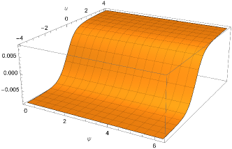
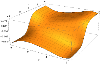
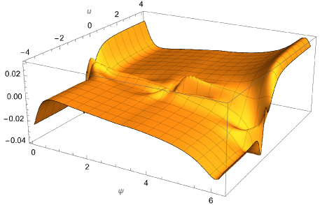
Figure 2: Waveform of $h^{\infty}_{+}$ at $a/b={0.0}$, $a/b={0.2}$, $a/b={0.65}$.

Figure 3: Waveform of $h^{\infty}_{+}\,\,$ for different values of $a/b$ with spin angle $\psi{=}{\pi\over 4}$.

From the waveform, we can extract the gravitational memory effect using

$$\Delta h^{\infty}=h^{\infty}(+\infty)-h^{\infty}(-\infty).$$ (6.37)

We first study the Taylor expansion around $u\rightarrow\infty$ of the individual pieces $h^{\infty}_{i}(u)$ which contribute to the waveform in (6.33) and find they all have similar behaviour

$$h^{\infty}_{i}(u)\sim c_{i}+\mathcal{O}\Big{(}{1\over u}\Big{)}.$$ (6.38)

The contributions $h_{1}^{\infty}$ and $h_{2}^{\infty}$ have the derivative $i\partial_{u}$ acting on them as such their behaviour in the large $u$ limit is sub-leading and they do not contribute to the memory. The memory can then by computed from the contribution $h_{0}^{\infty}$ and we find

$$\Delta h^{\infty} =\frac{\kappa^{4}m_{1}m_{2}}{8\pi}\frac{v_{1}{\cdot}F_{k}{\cdot}v_{2}}{4w_{1}^{2}w_{2}^{2}\sqrt{y^{2}-1}\left(4\left(a_{1}{\cdot}b\right){}^{2}+\left(a_{1}{\cdot}a_{1}+1\right){}^{2}\right)}$$

$$\times\Big{(}2a_{1}{\cdot}bv_{1}{\cdot}F_{k}{\cdot}v_{2}\left(\left(1-2y^{2}\right)a_{1}{\cdot}k+w_{0}y\left(a_{1}{\cdot}a_{1}-1\right)\right)$$

$$+4w_{2}a_{1}{\cdot}b\left(\left(1-2y^{2}\right)a_{1}{\cdot}F_{k}{\cdot}v_{1}+y\left(a_{1}{\cdot}a_{1}-1\right)v_{\perp}{\cdot}F_{k}{\cdot}v_{1}\right)$$

$$-\left(a_{1}{\cdot}a_{1}+1\right)\left(-2w_{2}b{\cdot}F_{k}{\cdot}v_{1}+w_{3}v_{1}{\cdot}F_{k}{\cdot}v_{2}\right)\left(2yv_{2}{\cdot}S_{1}{\cdot}b+2y^{2}-1\right)\Big{)}.$$ (6.39)

In this compact formula, we notice that all the terms contain at least one pole in $w_{1}$ and $w_{2}$. This indicates that contact terms in the Compton amplitude do not contribute to the memory at any order in spin. As such we should expect that the waveform we have computed fully captures the memory to all orders in the spin. In addition, we compute a formula for the tree-level gravitational memory at all orders in spin (8.36) in Section 8 below using a classical soft factor. The two formulae are indeed in agreement. We also mention again that we have compared our results to those of [157], finding agreement (see also [164]).

A graph of the memory, for the same kinematics as before and various values of the magnitude of the spin and direction, is presented in Figure 4. When $|a|$ tends to 1, there are two singular points at $\psi=0,\pi$ corresponding to when the spin vector and impact parameter are orthogonal.

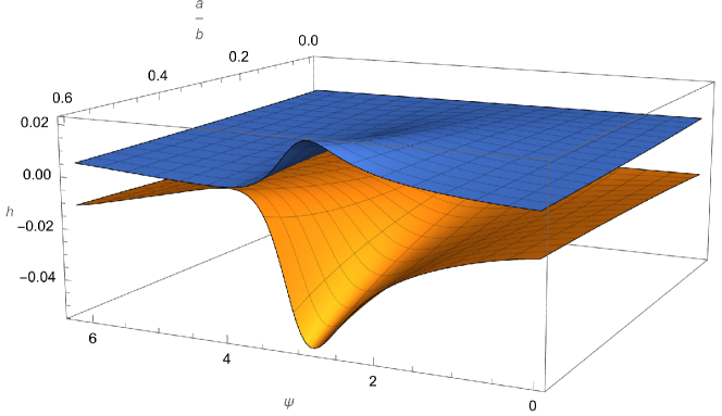
Figure 4: Gravitational memory: the top graph (blue) is the imaginary part, corresponding to $h^{\infty}_{\times}$, and the bottom graph (orange) is the real part, corresponding to $h^{\infty}_{+}$.

7 Comparison with the spin-expanded waveforms

If the spin parameter is small with respect to the impact parameter $a\ll|b|$ then we can evaluate the waveform integration order by order in a spin expansion. When we perform such an expansion the tree-level five-point amplitude is free of the spin-dependent spurious poles. One can still work in the $q_{1}^{2}$ and $q_{2}^{2}$ channels separately, which only contain one spurious pole $\frac{1}{q_{1}{\cdot}k}$. After the usual re-scaling $q_{i}=\omega\hat{q}_{i}$, the waveform integrand is given by

$$\mathcal{M}_{q_{1}^{2}}={1\over\omega^{2}}\Big{(}\sum_{i=0}^{\infty}\mathcal{M}^{(i)}_{q_{1}^{2}}\omega^{i}\Big{)}, \mathcal{M}_{q_{2}^{2}}={1\over\omega^{2}}\Big{(}\sum_{i=0}^{\infty}\mathcal{M}^{(i)}_{q_{2}^{2}}\omega^{i}\Big{)}.$$ (7.1)

We still integrate over the frequency first but now after expanding in the spin parameter there is only one sector per cut. Thus the integrand contains the same delta functions as in the scalar case

$$\begin{cases}\quad\delta\left(-b{\cdot}\hat{q}_{1}+u\right)&q_{1}^{2}\text{-channel,}\\ \quad\delta\left(-b{\cdot}\hat{q}_{2}+u\right)&q_{2}^{2}\text{-channel}.\end{cases}$$ (7.2)

The extra powers of $\omega$ become derivatives in the retarded time, $i\partial_{u}$, as before. Now using the original parameterisation (5.20), after we localise $z_{b}$ each term in the integrand belongs to one of the following general expressions

$${c_{0}+c_{1}z_{v}+c_{2}z_{v}^{2}+c_{3}z_{v}^{3}+\cdots\over(z_{v}+\tilde{c})(z_{v}^{2}+\bar{c})}, {\bar{c}_{0}+\bar{c}_{1}z_{v}+\bar{c}_{2}z_{v}^{2}+\bar{c}_{3}z_{v}^{3}+\cdots\over(z_{v}^{2}+\bar{c})}\,,$$ (7.3)

where the $c$’s are functions of the external kinematics. The ${1\over z_{v}^{2}+c^{\prime}_{2}}$ is the physical $q_{1}^{2}$ (or $q_{2}^{2}$) pole and ${1\over z_{v}+c^{\prime}_{1}}$ is the spurious pole at $q_{1}{\cdot}k$. Since the waveform only receives contributions from the physical pole, we can use polynomial division to reduce the numerators. Explicitly, we perform polynomial division over the physical pole, and obtain

$${c^{\prime}_{0}+c^{\prime}_{1}z_{v}\over(z_{v}+\tilde{c})(z_{v}^{2}+\bar{c})}+(\text{terms without physical poles}),$$

$${\bar{c}^{\prime}_{0}+\bar{c}^{\prime}_{1}z_{v}\over(z_{v}^{2}+\bar{c})}+(\text{terms without physical poles}).$$ (7.4)

Terms without physical poles correspond to contributions that are proportional to delta functions in $b$ (and derivatives thereof) and hence do not contribute to the long-range waveform. Thus we only have the following two types of master integrals after performing partial fractions over the spurious pole

$${c^{{}^{\prime\prime}}_{0}\over(z_{v}+\tilde{c})(z_{v}^{2}+\bar{c})}\,,$$

$${\bar{c}^{{}^{\prime\prime}}_{0}+\bar{c}^{{}^{\prime\prime}}_{1}z_{v}\over(z_{v}^{2}+\bar{c})}={\bar{c}^{{}^{\prime\prime}}_{0}\over(z_{v}^{2}+\bar{c})}+\text{(terms that integrate to zero)}.$$ (7.5)

The two master integrals can then be evaluated by calculating the residue on the physical pole. The final result of the $q_{1}$ integral is of the form

$$h^{\infty}_{\rm expanded}(u) =\Big{(}\sum_{i=0}^{\infty}\omega^{i}h^{\infty}_{i}(u)\Big{)}|_{\omega\rightarrow i\partial_{u}}$$

$$\sim\Bigg{[}\frac{\omega^{4}a_{1}{\cdot}a_{1}a_{1}{\cdot}\hat{k}\,v_{\perp}{\cdot}F_{\hat{k}}{\cdot}v_{1}\,a_{1}{\cdot}F_{\hat{k}}{\cdot}v_{1}}{24\left(y^{2}-1\right)}-\frac{i\omega^{3}a_{1}{\cdot}a_{1}\,v_{\perp}{\cdot}F_{\hat{k}}{\cdot}v_{1}\text{tr}\left(F_{\hat{k}},S_{1}\right)}{48\left(y^{2}-1\right)}$$

$$-\frac{\hat{w}_{0}\left(2y^{2}-1\right)\left(v_{1}{\cdot}F_{\hat{k}}{\cdot}v_{2}\right){}^{2}}{8\hat{w}_{1}^{2}\hat{w}_{2}^{2}\left(y^{2}-1\right)}-\frac{\left(2y^{2}-1\right)\left(v_{1}{\cdot}F_{\hat{k}}{\cdot}v_{2}\right){}^{2}}{8\hat{w}_{1}^{2}\hat{w}_{2}^{2}\left(y^{2}-1\right)\sqrt{-u^{2}\left(y^{2}-1\right)-\hat{w}_{2}^{2}}}$$

$$\times\left(-\hat{w}_{0}\sqrt{u^{2}\left(-y^{2}\right)+u^{2}-\hat{w}_{2}^{2}}+u\hat{w}_{3}y^{2}-u\hat{w}_{3}+\hat{w}_{1}\hat{w}_{2}y-\hat{w}_{2}^{2}\right)$$

$$+\cdots\text{more terms}\cdots\Bigg{]}\Bigg{|}_{\omega\rightarrow i\partial_{u}}.$$ (7.6)

The full waveform result expanded in the spin parameter up to $a^{4}$ order is included in the GitHub repository. Our result contains contributions at orders beyond $a^{4}$ but these will in general be incomplete until possible additional contact terms are included in the Compton amplitude.

We now comment on the difference between the resummed spinning waveform versus the spin-expanded waveform truncated at $\mathcal{O}(a^{4})$. To do so, we illustrate the spin-expanded waveform at $a/b=0.2$ and $a/b=0.65$ in Figure 5. Comparing with the resummed result shown for the same values in Figure 2, we see that for $a/b=0.2$ the spin-expanded result at $\mathcal{O}(a^{4})$ is accurate. However, at $a/b=0.65$ the spin expansion breaks down and the perturbative result is no longer valid.

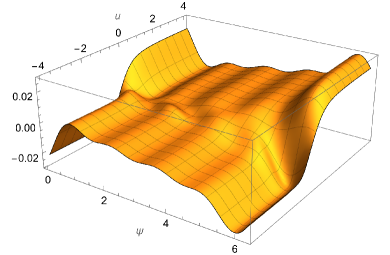
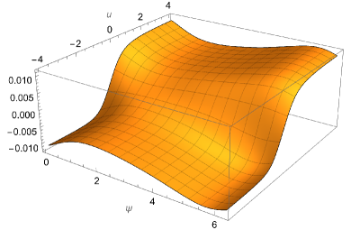
Figure 5: Waveform of $h^{+}$ at $a/b={0.65}$, $a/b={0.2}$.

To see more clearly the difference between the resummed spin result and the perturbative spin result truncated at $\mathcal{O}(a^{4})$, we also fix $\psi={\pi\over 4}$. For lower values of spin, for example $a/b={0.2}$, the expanded and resummed waveforms are nearly identical, as shown in the right-hand side of Figure 6. Conversely, for large values of the spin, for example $a/b={0.65}$, the expanded and resummed results are markedly different, although their limiting values as $u\rightarrow\pm\infty$ are similar.

Figure 6: Comparison of the expanded and resummed waveforms $h_{+}$ at $a/b=0.65$ and $a/b=0.2$ with spin angle $\psi={\pi\over 4}$. For $a/b=0.2$ the graphs are indistinguishable.

The above comparisons between our expanded and resummed waveforms require a number of considerations. For physical black holes we require $a/Gm\ll 1$, and additionally, in the PM expansion we require $Gm/b\ll 1$. For the case of large spin $a$, for example $a/b=0.65$ plotted above, it is clear that only one of the ratios, $Gm/b$ or $a/Gm$, can be taken as small. If we consider physical black holes, $a/Gm\ll 1$, then $Gm/b$ is no longer small, and we require higher orders in the PM expansion to reliably reproduce the physical waveform. Thus the plots in Figure 6 would then change significantly once we include such terms. Alternatively, we could consider again the case where $a{\sim}b$ but now require that $Gm/b\ll 1$ such that we only need consider low orders in the PM expansion. In this case, we must again resum in the spin parameter $a/b$, but now we are in fact considering super-extremal Kerr, $a/Gm\gg 1$. Figure 6 much more accurately reproduces the waveform in this regime, and we see that resuming in spin substantially changes the waveform.

Finally, we also remind the reader that the results presented in this paper are valid up to $\mathcal{O}(a^{4})$, as discussed in Section 3.2.

8 Gravitational memory

8.1 General strategy

An elegant way to compute the memory was discussed in [114] for the spinless case, and we adapt it to the case of spinning heavy particles. Given a function

$$f(u)\coloneqq\int_{-\infty}^{+\infty}\!\frac{d\omega}{2\pi}e^{-i\omega u}\tilde{f}(\omega)$$ (8.1)

of the retarded time $u$, the memory is defined as

$$\begin{split}\Delta f&\coloneqq f(u\to+\infty)-f(u\to-\infty)=\int_{-\infty}^{+\infty}\!du\,\frac{d}{du}f(u)\\ &=-i\int_{-\infty}^{+\infty}\!{d\omega}\,\delta({\omega})\big{[}\omega\tilde{f}(\omega)\big{]}\,,\end{split}$$ (8.2)

showing that it is determined by the pole at $\omega{=}0$, i.e. its soft limit, as observed by [165].

We now apply (8.2) to (5.13) to compute the gravitational memory, getting

$$\Delta(h^{\infty}_{+}\pm ih^{\infty}_{\times})=-i\frac{\kappa}{2}\left[\lim_{\omega\to 0^{+}}\big{[}\omega W\big{(}b,k^{\pm}\big{)}\big{]}_{k=\omega(1,\mathbf{\hat{x}})}+\lim_{\omega\to 0^{-}}\big{[}\omega W^{\ast}\big{(}b,k^{\mp}\big{)}\big{]}_{k=-\omega(1,\mathbf{\hat{x}})}\right]\,.$$ (8.3)

From this relation we see that the memory effect arises from the leading soft behaviour of the five-point amplitude, which factorises into a soft factor times a four-point amplitude, schematically

$$\mathcal{M}_{5}\rightarrow{\rm Soft}\times\mathcal{M}_{4}.$$ (8.4)

Correspondingly, as $\omega\to 0$ the waveform tends to its leading soft limit,

$$W_{\rm soft}\big{(}b,k^{h}\big{)}=-i\int\!d\mu^{(D)}e^{iq{\cdot}b}S_{\rm W}^{\rm HEFT}(k,q;h)\mathcal{M}_{4}^{\rm HEFT}(q)\,,$$ (8.5)

where [62]

$$\begin{split}S_{\rm W}^{\rm HEFT}&=-\frac{\kappa}{2}\,\varepsilon_{\mu\nu}^{(h)}(k)\left[\frac{p_{1}^{\mu}q^{\nu}+p_{1}^{\nu}q^{\mu}}{p_{1}{\cdot}k}-p_{1}^{\mu}p_{1}^{\nu}\frac{q{\cdot}k}{(p_{1}{\cdot}k)^{2}}\,-\,1\leftrightarrow 2\right]\\ &=-\frac{\kappa}{2}\,\frac{1}{\omega}\varepsilon_{\mu\nu}^{(h)}(k)\left[\frac{p_{1}^{\mu}q^{\nu}+p_{1}^{\nu}q^{\mu}}{p_{1}{\cdot}\hat{k}}-p_{1}^{\mu}p_{1}^{\nu}\frac{q{\cdot}\hat{k}}{(p_{1}{\cdot}\hat{k})^{2}}\,-\,1\leftrightarrow 2\right]\,,\,\end{split}$$ (8.6)

is the classical Weinberg soft factor for the emission of a graviton with momentum $k{=}\omega\hat{k}$ and helicity $h$, with $q{=}q_{1}{=}-q_{2}$ in the soft limit and $\hat{k}{=}(1,\mathbf{\hat{x}})$ (see [62] for a derivation of the classical soft factor and a discussion of classical limits in the HEFT context).

We then change integration variables $q{\to}-q$, and use

$$S_{\rm W}^{\rm HEFT}(-k,-q;h) =S_{\rm W}^{\rm HEFT}(k,q;h)\,,$$ (8.7)

$$\big{[}S_{\rm W}^{\rm HEFT}(k,q,-h)\big{]}^{\ast} =S_{\rm W}^{\rm HEFT}(k,q,h)\,,$$ (8.9)

also noting that, at tree level in the spinning (and spinless) case,

$$-i\mathcal{M}_{4}^{\rm HEFT}(q)=\big{[}-i\mathcal{M}_{4}^{\rm HEFT}(-q)\big{]}^{\ast}\,,$$ (8.10)

which can be checked from the explicit expression derived later in (8.26). With these observations, we get

$$\begin{split}\left.W_{\rm soft}^{\ast}\big{(}b,k^{-h}\big{)}\right|_{k=-\omega(1,\hat{\mathbf{x}})}&=\int\!d\mu^{(D)}e^{-iq{\cdot}b}\big{[}S_{\rm W}^{\rm HEFT}(-k,q;-h)\big{]}^{\ast}(-i\mathcal{M}_{4}^{\rm HEFT})^{\ast}(q)\\ &=\int\!d\mu^{(D)}e^{iq{\cdot}b}S_{\rm W}^{\rm HEFT}(-k,-q;h)(-i\mathcal{M}_{4}^{\rm HEFT})^{\ast}(-q)\\ &=\int\!d\mu^{(D)}e^{iq{\cdot}b}S_{\rm W}^{\rm HEFT}(k,q;h)(-i\mathcal{M}_{4}^{\rm HEFT})(q)\,.\end{split}$$ (8.11)

Hence we can write

$$\begin{split}&\lim_{\omega\to 0^{+}}\big{[}\omega W\big{(}b,k^{h}\big{)}\big{]}_{k=\omega(1,\mathbf{\hat{x}})}+\lim_{\omega\to 0^{-}}\big{[}\omega W^{\ast}\big{(}b,k^{-h}\big{)}\big{]}_{k=-\omega(1,\mathbf{\hat{x}})}\\ &=\int\!d\mu^{(D)}e^{iq_{\cdot}b}S_{\rm W}^{\rm HEFT}(\hat{k},q;h)(-i\mathcal{M}_{4}^{\rm HEFT})\,.\end{split}$$ (8.12)

In conclusion

$$\begin{split}\Delta(h^{\infty}_{+}\pm ih^{\infty}_{\times})&=-i\,\kappa\int\!d\mu^{(D)}e^{iq_{\cdot}b}S_{\rm W}^{\rm HEFT}(\hat{k},q;\pm)\,\big{(}-i\mathcal{M}_{4}^{\rm HEFT}\big{)}(q)\\ &=-i\,\kappa S_{\rm W}^{\rm HEFT}\Big{(}\hat{k},-i\frac{\partial}{\partial b};\pm\Big{)}\int\!d\mu^{(D)}e^{iq{\cdot}b}\,\,\big{(}-i\mathcal{M}_{4}^{\rm HEFT}\big{)}(q)\\ &=-i\,\kappa S_{\rm W}^{\rm HEFT}\Big{(}\hat{k},-i\frac{\partial}{\partial b};\pm\Big{)}\,\delta_{\rm HEFT}\,,\end{split}$$ (8.13)

or

$$\begin{split}\Delta(h^{\infty}_{+}\pm ih^{\infty}_{\times})&=-i\,\kappa S_{\rm W}^{\rm HEFT}\Big{(}\hat{k},-i\frac{\partial}{\partial b};\pm\Big{)}\,\delta_{\rm HEFT}\,,\end{split}$$ (8.14)

where

$$\delta_{\rm HEFT}\coloneqq\int\!d\mu^{(D)}e^{iq_{\cdot}b}\,\big{(}-i\mathcal{M}_{4}^{\rm HEFT}\big{)}(q)\,,$$ (8.15)

and $S_{\rm W}^{\rm HEFT}$ is given in (8.6), and we also recall that $k{=}\omega\hat{k}$. Note that $\delta_{\rm HEFT}$ is real because of the property (8.9).

In the spinless case, one can further simplify this result by noticing that

$$\frac{\partial}{\partial b_{\mu}}{=}-P\hat{b}^{\mu}\frac{\partial}{\partial J}\,,$$ (8.16)

where $J=P\sqrt{-b^{2}}$, and the relation between the scattering angle and the real part of the HEFT phase

$$-\frac{\partial}{\partial J}\,{\rm Re}\,\delta_{\rm HEFT}=\chi,\,$$ (8.17)

which itself is already a real quantity at tree level. Using these one finds

$$S_{\rm W}^{\rm HEFT}\Big{(}\hat{k},-i\frac{\partial}{\partial b_{\mu}};h\Big{)}\,\delta_{\rm HEFT}=-iPS_{\rm W}^{\rm HEFT}(\hat{k},\hat{b}^{\mu};h)\chi\,,$$ (8.18)

leading to the compact relation, valid in the spinless case,

$$\begin{split}\Delta(h^{\infty}_{+}\pm ih^{\infty}_{\times})&=-\frac{\kappa^{2}}{2}P\varepsilon_{\rho\lambda}^{\pm\pm}s^{\rho\lambda}(\hat{k},\hat{b})\,\chi\,,\end{split}$$ (8.19)

where we have set

$$\begin{split}S_{\rm W}^{\rm HEFT}&\coloneqq\frac{\kappa}{2}\varepsilon_{\rho\lambda}^{\pm\pm}s^{\rho\lambda}(\hat{k},\hat{b})\\ s^{\mu\nu}(\hat{k},\hat{b})&=-\Big{[}\frac{p_{1}^{\mu}\hat{b}^{\nu}+p_{1}^{\nu}\hat{b}^{\mu}}{p_{1}{\cdot}\hat{k}}-p_{1}^{\mu}p_{1}^{\nu}\frac{\hat{b}{\cdot}\hat{k}}{(p_{1}{\cdot}\hat{k})^{2}}\,-\,1\leftrightarrow 2\Big{]}\,,\end{split}$$ (8.20)

and we recall that $\hat{k}=(1,\mathbf{\hat{x}})$ and $\hat{b}=b/\sqrt{-b^{2}}$. In the spinning case we do not have a simple relation such as (8.17) and we will instead make use of (8.14). To compute the gravitational memory in the spinning case we will then use (8.14) and (8.15).

We now move on to compute the tree-level-four-point amplitude that features in (8.15).

8.2 Four-point two-to-two spinning amplitude

In this section we derive the tree-level amplitude for the two-to-two scattering of two heavy particles with spin vectors $a_{1}$ and $a_{2}$ to all orders in the spin. We will then compute its Fourier transform to impact parameter space needed in (8.15).

We can derive the four-point amplitude using the HEFT BCFW method first described in [62], to which we refer the reader for further details. There is a single diagram in the $q^{2}$-channel for which we glue two of the three point amplitudes (3.2) with the BCFW-shifted momenta described in [62]. We find that the four-point tree-level amplitude $\mathcal{M}_{4}$ is then

$$\begin{split}\mathcal{M}_{4}&=-{i\frac{\kappa^{2}}{q^{2}}}m_{1}^{2}m_{2}^{2}\Big{[}\Big{(}y^{2}-\frac{1}{2}\Big{)}\cosh\left(a{\cdot}q\right)\\ &+\,i\,y\Big{(}\sinh\left(a_{2}{\cdot}q\right)\cosh\left(a_{1}{\cdot}q\right)\frac{\epsilon\left(a_{2}qv_{1}v_{2}\right)}{a_{2}{\cdot}q}+\sinh\left(a_{1}{\cdot}q\right)\cosh\left(a_{2}{\cdot}q\right)\frac{\epsilon\left(a_{1}qv_{1}v_{2}\right)}{a_{1}{\cdot}q}\Big{)}\Big{]}\\ &+\mathcal{M}_{4,c}\,,\end{split}$$ (8.21)

where $a{\coloneqq}a_{1}+a_{2}$, and the contact term $\mathcal{M}_{4,c}$ is

$$\mathcal{M}_{4,c}\coloneqq-i\kappa^{2}m_{1}^{2}m_{2}^{2}\Big{[}y\,a_{1}{\cdot}v_{2}\,a_{2}{\cdot}v_{1}-a_{1}{\cdot}a_{2}\Big{(}y^{2}-{1\over 2}\Big{)}\Big{]}{\frac{\sinh(a_{1}{\cdot}q)}{a_{1}{\cdot}q}}{\frac{\sinh(a_{2}{\cdot}q)}{a_{2}{\cdot}q}}\,.$$ (8.22)

We note however that contact terms play no role for the computation of the memory, since they only contribute delta-function supported terms after Fourier transforming to impact parameter space. We will then drop them from now on (denoting the contact terms as $\mathcal{O}(1)$).

We now simplify the expression (8.21) for the four-point amplitude making use of the new spin vectors [43, 123]

$$\mathfrak{a}^{\mu}_{i}\coloneqq\frac{\epsilon(a_{i}\mu v_{1}v_{2})}{\sqrt{y^{2}-1}}\,,\quad i=1,2,$$ (8.23)

which are orthogonal to both $v_{1}$ and $v_{2}$. These quantities also satisfy the following Gram determinant relations

$$(a_{i}{\cdot}q)^{2}=({i\mathfrak{a}_{i}{\cdot}q})^{2}+\mathcal{O}(q^{2})\,,$$ (8.24)

which are proven in Appendix A, and their “square rooted” form

$$a_{i}{\cdot}q=\pm{i\mathfrak{a}_{i}{\cdot}q}\,,$$ (8.25)

valid up to terms of $\mathcal{O}(q^{2})$, that is $q$ on-shell and so necessarily complex. Furthermore, as both $\cosh(a_{i}{\cdot}q)$ and ${\sinh(a_{i}{\cdot}q)\over a_{i}{\cdot}q}$ are parity-even functions of $a_{i}{\cdot}q$, the sign ambiguity drops out and the amplitude can be simplified to

$$\begin{split}\mathcal{M}_{4}&=-{i\kappa^{2}\over q^{2}}{m_{1}^{2}m_{2}^{2}}\Big{\{}\Big{(}y^{2}-\frac{1}{2}\Big{)}\cosh({i\mathfrak{a}{\cdot}q})+y{\sqrt{y^{2}-1}}\sinh({i\mathfrak{a}{\cdot}q})\Big{\}}+\mathcal{O}(1)\,\\ &=-{i\kappa^{2}\over q^{2}}{m_{1}^{2}m_{2}^{2}\over 2}\Big{\{}\Big{(}y^{2}-\frac{1}{2}+y{\sqrt{y^{2}-1}}\Big{)}e^{{i\mathfrak{a}{\cdot}q}}+\Big{(}y^{2}-\frac{1}{2}-y{\sqrt{y^{2}-1}}\Big{)}e^{-{i\mathfrak{a}{\cdot}q}}\Big{\}}\\ &+\mathcal{O}(1)\,,\end{split}$$ (8.26)

where

$$\mathfrak{a}{\coloneqq}\mathfrak{a}_{1}{+}\mathfrak{a}_{2}\ .$$ (8.27)

Note the nontrivial fact that at tree level the pole part of the amplitude that we have considered so far depends only on the sum $\mathfrak{a}$ of the spins of the two heavy particles. We also remark that the contact term (8.22) does not have this property.

8.3 Fourier transform to impact parameter space

Having cast the amplitude (up to contact terms) in the form (8.26), we can perform the Fourier transform to impact parameter space to all orders in the spin, which will trivially shift $b^{\mu}\to b^{\mu}\pm\mathfrak{a}$, as was seen in [123]. We have

$$\widetilde{\mathcal{M}}_{4}=\int\!\frac{d^{D}q}{(2\pi)^{D-2}}\delta(2p_{1}{\cdot}q)\delta(2p_{2}{\cdot}q)\,e^{iq{\cdot}b}\,\mathcal{M}_{4}=\frac{1}{4m_{1}m_{2}\sqrt{y^{2}-1}}\int\!\frac{d^{D-2}q_{\perp}}{(2\pi)^{D-2}}e^{-i\vec{q}_{\perp}{\cdot}\vec{b}}\,{\mathcal{M}}_{4}\,,$$ (8.28)

where $q_{\perp}{\cdot}p_{1,2}{=}0$ and

$$\mathcal{M}_{4}=f_{+}(y)\frac{e^{i\mathfrak{a}{\cdot}q}}{q^{2}}+f_{-}(y)\frac{e^{-i\mathfrak{a}{\cdot}q}}{q^{2}}\,,$$ (8.29)

with

$$f_{\pm}(y)\coloneqq\ -i\,\frac{\kappa^{2}m_{1}^{2}m_{2}^{2}}{2}\left(y^{2}-\frac{1}{2}\pm y\sqrt{y^{2}-1}\right)\,.$$ (8.30)

Thus, we have to compute the Fourier transform

$$\widetilde{\mathcal{M}}_{4}=\int\!\frac{d^{D}q}{(2\pi)^{D-2}}\delta(2p_{1}{\cdot}q)\delta(2p_{2}{\cdot}q)\,\left[e^{iq{\cdot}(b+\mathfrak{a})}f_{+}(y)+e^{iq{\cdot}(b-\mathfrak{a})}f_{-}(y)\right]\,.$$ (8.31)

We use

$$\int\!\frac{d^{d}q}{(2\pi)^{d}}e^{-i\vec{q}{\cdot}\vec{b}}|\vec{q}\,|^{p}=\frac{2^{p}\pi^{-\frac{d}{2}}\Gamma\left(\frac{d+p}{2}\right)}{\Gamma\left(-\frac{p}{2}\right)}\frac{1}{|\vec{b}\,|^{d+p}}\,,$$ (8.32)

which in our case gives the result, as $D\to 4$,

$$\int\!\frac{d^{D-2}q}{(2\pi)^{D-2}}\frac{e^{-i\vec{q}{\cdot}\vec{b}}}{\vec{q}^{\,2}}=\frac{\Gamma\left(\frac{D-4}{2}\right)}{4\pi^{\frac{D-2}{2}}|\vec{b}\,|^{D-4}}\xrightarrow[D\to 4]{}-\frac{1}{2\pi}\log(|\vec{b}\,|)+\cdots\,,$$ (8.33)

where the dots stand for $b$-independent terms. This leads to

$$\widetilde{\mathcal{M}}_{4}=\frac{1}{8\pi m_{1}m_{2}\sqrt{y^{2}-1}}\Big{[}f_{+}(y)\log(|b+\mathfrak{a}|)+f_{-}(y)\log(|b-\mathfrak{a}|)\Big{]}+\cdots\,,$$ (8.34)

where we observe that the vector $\mathfrak{a}{=}\mathfrak{a}_{1}+\mathfrak{a}_{2}$ lives in the same two-dimensional subspace orthogonal to $p_{1}$ and $p_{2}$ as $b$. (8.34) agrees with (51) of [123].

8.4 Result for the gravitational memory

Finally, to compute the gravitational memory we use (8.14) and (8.15). Introducing the two vectors

$$b_{\pm}\coloneqq b\pm\mathfrak{a}\,,\qquad\text{with}\qquad\hat{b}_{\pm}\coloneqq\frac{b_{\pm}}{|b_{\pm}|}\,,$$ (8.35)

we have at once

$$\begin{split}\Delta(h^{\infty}_{+}\pm ih^{\infty}_{\times})&=-\frac{i\kappa}{8\pi m_{1}m_{2}\sqrt{y^{2}-1}}\Big{[}S_{\rm W}^{\rm HEFT}(\hat{k},\hat{b}_{+};\pm)\frac{f_{+}(y)}{|b_{+}|}+S_{\rm W}^{\rm HEFT}(\hat{k},\hat{b}_{-};\pm)\frac{f_{-}(y)}{|b_{-}|}\Big{]}\end{split},$$ (8.36)

which is the final result for the memory, with $S_{\rm W}^{\rm HEFT}$ defined in (8.20) and $f_{\pm}$ in (8.30). This result is exact to all orders in the spin vector $a$. One can expand it to various order in $a$, and doing so one finds perfect agreement with the result of [151] for the memory in the aligned spin case up to $\mathcal{O}(a^{2})$.

We also note that in the spinless case, the previous formula becomes

$$\begin{split}\left.\Delta(h^{\infty}_{+}\pm ih^{\infty}_{\times})\right|_{a=0}&=-\frac{i\kappa}{8\pi m_{1}m_{2}\sqrt{y^{2}-1}}(-i\kappa^{2}m_{1}^{2}m_{2}^{2})\frac{1}{|b|}\Big{(}y^{2}-\frac{1}{2}\Big{)}S_{\rm W}^{\rm HEFT}(\hat{k},\hat{b};\pm)\\ &=-\frac{\kappa^{3}}{8\pi}\frac{m_{1}m_{2}}{\sqrt{y^{2}-1}}\frac{1}{|b|}\Big{(}y^{2}-\frac{1}{2}\Big{)}S_{\rm W}^{\rm HEFT}(\hat{k},\hat{b};\pm)\,,\end{split}$$ (8.37)

in agreement with known results (see e.g. [151]).

Appendix A Simplifying the four-point amplitude

In the main text we have defined a new spin vector (8.23), and $\mathfrak{a}\coloneqq\mathfrak{a}_{1}+\mathfrak{a}_{2}$ which are all orthogonal to both $v_{1}$ and $v_{2}$. Now from the square of the Levi-Civita tensor we obtain a Gram determinant, for $i=1,2$,

$$\big{[}\epsilon(a_{i}qv_{1}v_{2})\big{]}^{2}={(a_{i}{\cdot}q)^{2}\over 1-y^{2}}+q^{2}\Big{[}(a_{i}{\cdot}v_{1})^{2}+(a_{i}{\cdot}v_{2})^{2}-2y\,a_{i}{\cdot}v_{1}a_{i}{\cdot}v_{2}+a_{i}^{2}(y^{2}-1)\Big{]}\,,$$ (A.1)

valid with the HEFT constraints $v_{1,2}{\cdot}q{=}0$. Using that $v_{i}{\cdot}a_{i}{=}0$ we then find

$$\begin{split}\big{[}\epsilon\left(a_{1}qv_{1}v_{2}\right)\big{]}^{2}&=-{(a_{1}{\cdot}q)^{2}\over y^{2}-1}+q^{2}\Big{(}(a_{1}{\cdot}v_{2})^{2}+a_{1}^{2}(y^{2}-1)\Big{)}\,,\\ \big{[}\epsilon\left(a_{2}qv_{1}v_{2}\right)\big{]}^{2}&=-{(a_{2}{\cdot}q)^{2}\over y^{2}-1}+q^{2}\Big{(}(a_{2}{\cdot}v_{1})^{2}+a_{2}^{2}(y^{2}-1)\Big{)}\,.\end{split}$$ (A.2)

In the calculation in impact parameter space, $\mathcal{O}(q^{2})$ terms do not contribute, giving (8.24) in the main text.

To simplify the four-point amplitude we actually used the square root of the above relations, that is

$$\frac{\epsilon\left(a_{2}qv_{1}v_{2}\right)}{a_{2}{\cdot}q}=\frac{\epsilon\left(a_{1}qv_{1}v_{2}\right)}{a_{1}{\cdot}q}=\mp i\sqrt{y^{2}-1}+\mathcal{O}(q^{2})\,,$$ (A.3)

which are again valid up to terms order $\mathcal{O}(q^{2})$. Since the amplitude is parity even, the sign ambiguity in these relations drops out.

One might ask what determines the sign on the right-hand side of (A.3). A simple way to answer this question is to go to the rest frame of particle one, and show that the $\mp$ sign in (A.3) follows the particular choice of the on-shell momentum $q$. We can set

$$v_{1}=(1,0,0,0)\,,\qquad v_{2}=(y,0,0,\sqrt{y^{2}-1})\,.$$ (A.4)

Now, $q$ is on-shell, $q^{2}{=}0$, and satisfies the usual constraints $q{\cdot}v_{1}{=}q{\cdot}v_{2}=0$, hence it must have the form

$$q=(0,r,\pm ir,0)\,.$$ (A.5)

Finally, using $a_{1}{\cdot}v_{1}=0$ and $a_{2}{\cdot}v_{2}=0$, the spin vectors are of the form

$$\begin{split}a_{1}&=(0,a_{1x},a_{1y},a_{1z})\,,\\ a_{2}&=\Big{(}{s\over y},a_{2x},a_{2y},{s\over\sqrt{y^{2}-1}}\Big{)}\,,\end{split}$$ (A.6)

and hence we can evaluate, for $i=1,2$,

$$\begin{split}\epsilon(v_{1}v_{2}a_{i}q)&=\epsilon(\vec{v}_{2}\vec{a}_{i}\vec{q})=\pm\sqrt{y^{2}-1}\,r\,(ia_{ix}\mp a_{iy})\,,\\ a_{i}{\cdot}q&=ir(ia_{ix}\mp a_{iy})\,.\end{split}$$ (A.7)

In conclusion

$$\frac{\epsilon(v_{1}v_{2}a_{i}q)}{a_{i}{\cdot}q}=\mp i\sqrt{y^{2}-1}\,,$$ (A.8)

with the same plus or minus sign appearing for $a_{1}$ or $a_{2}$ and following from the solution (A.5) chosen for the on-shell momentum $q$. Finally note that the right-hand side of (A.3) is manifestly imaginary, and the above discussion shows that the left-hand side of that equation is too.

Appendix B More on the integrand

In this appendix we provide the $c_{i}$ coefficients used in the formulae for the residues in each channel which appear in Sections 6.1 and 6.2. As in Section 6, in this appendix the $k,q_{i}$ and $w_{i}$ should be understood as the hatted quantities with all $\omega$ dependence scaled out and once again we drop these hats purely for conciseness. The $q^{2}_{1}$-channel coefficients in Section 6.1 are

$$\begin{split}&c_{1}\to-\frac{1}{2}\left(v_{1}{\cdot}F_{k}{\cdot}v_{2}\right){}^{2},\ c_{2}\to\frac{1-2y^{2}}{4w_{1}^{2}},\ c_{3}\to\frac{iy}{2w_{1}^{2}},\ c_{4}\to\frac{iyv_{1}{\cdot}F_{k}{\cdot}v_{2}}{2w_{1}^{2}},\\ &c_{5}\to-\frac{iyv_{1}{\cdot}F_{k}{\cdot}v_{2}}{2w_{1}^{2}},\ c_{6}\to\frac{yv_{1}{\cdot}F_{k}{\cdot}v_{2}}{w_{1}},\ c_{7}\to-\frac{iv_{1}{\cdot}F_{k}{\cdot}v_{2}}{2w_{1}},\ c_{8}\to-\frac{i\left(v_{1}{\cdot}F_{k}{\cdot}v_{2}\right){}^{2}}{2w_{1}},\\ &c_{9}\to-\frac{\left(2y^{2}-1\right)\left(v_{1}{\cdot}F_{k}{\cdot}v_{2}\right){}^{2}}{4w_{1}^{2}w_{2}^{2}},\ c_{10}\to-\frac{\left(2y^{2}-1\right)v_{1}{\cdot}F_{k}{\cdot}v_{2}}{2w_{1}^{2}w_{2}},\ c_{11}\to\frac{iy\left(v_{1}{\cdot}F_{k}{\cdot}v_{2}\right){}^{2}}{2w_{1}^{2}w_{2}^{2}},\\ &c_{12}\to\frac{iyv_{1}{\cdot}F_{k}{\cdot}v_{2}}{w_{1}^{2}w_{2}},\ c_{13}\to\frac{iy\left(v_{1}{\cdot}F_{k}{\cdot}v_{2}\right){}^{2}}{2w_{1}^{2}w_{2}},\ c_{14}\to\frac{y\left(v_{1}{\cdot}F_{k}{\cdot}v_{2}\right){}^{2}}{w_{1}w_{2}},\\ &c_{15}\to-\frac{i\left(v_{1}{\cdot}F_{k}{\cdot}v_{2}\right){}^{2}}{2w_{1}w_{2}},\ c_{16}\to-\frac{iw_{2}y}{2w_{1}^{2}},\ c_{17}\to\frac{iw_{2}v_{1}{\cdot}F_{k}{\cdot}v_{2}}{2w_{1}}\,.\end{split}$$ (B.1)

The coefficients in the $q^{2}_{2}$-channel, which appear in Section 6.2, are listed below:

$$c_{2} \to-\frac{1}{2}a_{1}{\cdot}a_{1}\left(v_{1}{\cdot}F_{k}{\cdot}v_{2}\right)^{2}$$

$$c_{4} \to\left(a_{1}{\cdot}v_{2}\right){}^{2}\left(a_{1}{\cdot}F_{k}{\cdot}v_{1}\right){}^{2}-\frac{1}{4}a_{1}{\cdot}a_{1}a_{1}{\cdot}F_{k}{\cdot}v_{1}\left(a_{1}{\cdot}F_{k}{\cdot}v_{1}-2a_{1}{\cdot}v_{2}v_{1}{\cdot}F_{k}{\cdot}v_{2}\right)$$

$$c_{5} \to\frac{1}{16}(-3)ia_{1}{\cdot}k\left(a_{1}{\cdot}a_{1}-2\left(a_{1}{\cdot}v_{2}\right){}^{2}\right)\text{tr}\left(F_{k}{\cdot}S_{1}\right),$$

$$c_{6} \to\frac{3}{16}i\left(a_{1}{\cdot}a_{1}-2\left(a_{1}{\cdot}v_{2}\right){}^{2}\right)\text{tr}\left(F_{k}{\cdot}S_{1}\right)a_{1}{\cdot}F_{k}{\cdot}v_{1},$$

$$c_{7} \to\frac{y\left(a_{1}{\cdot}v_{2}a_{1}{\cdot}F_{k}{\cdot}v_{1}+a_{1}{\cdot}a_{1}v_{1}{\cdot}F_{k}{\cdot}v_{2}\right)}{2w_{1}^{3}},$$

$$c_{10} \to\frac{a_{1}{\cdot}F_{k}{\cdot}v_{1}\left(2ya_{1}{\cdot}ka_{1}{\cdot}v_{2}+w_{1}\left(\left(a_{1}{\cdot}v_{2}\right){}^{2}+\left(y^{2}-1\right)a_{1}{\cdot}a_{1}\right)\right)}{4w_{1}^{3}},$$

$$c_{11} \to-\frac{\left(a_{1}{\cdot}F_{k}{\cdot}v_{1}\right){}^{2}+2a_{1}{\cdot}v_{2}v_{1}{\cdot}F_{k}{\cdot}v_{2}a_{1}{\cdot}F_{k}{\cdot}v_{1}+2a_{1}{\cdot}a_{1}\left(v_{1}{\cdot}F_{k}{\cdot}v_{2}\right){}^{2}}{4w_{1}^{2}},$$

$$c_{12} \to\frac{i\left(2y^{2}-1\right)\text{tr}\left(F_{k}{\cdot}S_{1}\right)}{8w_{1}^{2}},~{}~{}~{}~{}c_{13}\to\frac{\left(1-2y^{2}\right)\text{tr}\left(F_{k}{\cdot}S_{1}\right)a_{1}{\cdot}F_{k}{\cdot}v_{1}}{16w_{1}^{2}},$$

$$c_{14} \to-\frac{w_{1}a_{1}{\cdot}k\left(\left(a_{1}{\cdot}v_{2}\right){}^{2}+\left(y^{2}-1\right)a_{1}{\cdot}a_{1}\right)+y\left(a_{1}{\cdot}k\right){}^{2}a_{1}{\cdot}v_{2}+w_{1}^{2}ya_{1}{\cdot}a_{1}a_{1}{\cdot}v_{2}}{4w_{1}^{3}},$$

$$c_{15} \to\frac{a_{1}{\cdot}F_{k}{\cdot}v_{1}\left(ya_{1}{\cdot}k+w_{1}a_{1}{\cdot}v_{2}\right)}{4w_{1}^{2}},$$

$$c_{16} \to\frac{ya_{1}{\cdot}F_{k}{\cdot}v_{1}\left(2a_{1}{\cdot}v_{2}a_{1}{\cdot}F_{k}{\cdot}v_{1}+a_{1}{\cdot}a_{1}v_{1}{\cdot}F_{k}{\cdot}v_{2}\right)}{2w_{1}},$$

$$c_{19} \to-\frac{i\left(w_{1}a_{1}{\cdot}v_{2}v_{1}{\cdot}F_{k}{\cdot}v_{2}\text{tr}\left(F_{k}{\cdot}S_{1}\right)+a_{1}{\cdot}F_{k}{\cdot}v_{1}k{\cdot}S_{1}{\cdot}F_{k}{\cdot}v_{1}\right)}{4w_{1}},$$

$$c_{20} \to\frac{\text{tr}\left(F_{k}{\cdot}S_{1}\right)\left(\left(2y^{2}-1\right)a_{1}{\cdot}k+2w_{1}ya_{1}{\cdot}v_{2}\right)}{16w_{1}^{2}},$$

$$c_{21} \to\frac{\text{tr}\left(F_{k}{\cdot}S_{1}\right)\left(2ya_{1}{\cdot}ka_{1}{\cdot}v_{2}-w_{1}\left(a_{1}{\cdot}a_{1}-2\left(a_{1}{\cdot}v_{2}\right){}^{2}\right)\right)}{16w_{1}},$$

$$c_{22} \to-\frac{ya_{1}{\cdot}v_{2}\left(a_{1}{\cdot}F_{k}{\cdot}v_{1}\right){}^{2}}{4w_{1}^{3}},c_{25}\to\frac{iya_{1}{\cdot}F_{k}{\cdot}v_{1}}{2w_{1}^{2}},c_{26}\to-\frac{y\left(a_{1}{\cdot}F_{k}{\cdot}v_{1}\right)^{2}}{4w_{1}^{2}},$$

$$c_{29} \to-\frac{iyv_{1}{\cdot}F_{k}{\cdot}S_{1}{\cdot}v_{2}}{2w_{1}^{2}},c_{32}\to\frac{a_{1}{\cdot}F_{k}{\cdot}v_{1}}{8w_{1}},c_{33}\to-\frac{ia_{1}{\cdot}F_{k}{\cdot}v_{1}}{4w_{1}},c_{34}\to-\frac{a_{1}{\cdot}ka_{1}{\cdot}F_{k}{\cdot}v_{1}}{8w_{1}},$$

$$c_{35} \to-\frac{\left(a_{1}{\cdot}F_{k}{\cdot}v_{1}\right){}^{2}}{8w_{1}},c_{40}\to\frac{v_{1}{\cdot}F_{k}{\cdot}v_{2}a_{1}{\cdot}F_{k}{\cdot}v_{1}}{4w_{1}},c_{41}\to-\frac{iv_{1}{\cdot}F_{k}{\cdot}v_{2}a_{1}{\cdot}F_{k}{\cdot}v_{1}}{2w_{1}},$$

$$c_{43} \to\frac{iv_{1}{\cdot}F_{k}{\cdot}v_{2}v_{1}{\cdot}F_{k}{\cdot}S_{1}{\cdot}v_{2}}{2w_{1}},c_{44}\to\frac{3ia_{1}{\cdot}ka_{1}{\cdot}F_{k}{\cdot}v_{1}}{8w_{1}},c_{45}\to\frac{3ia_{1}{\cdot}ka_{1}{\cdot}v_{2}a_{1}{\cdot}F_{k}{\cdot}v_{1}}{4w_{1}},$$

$$c_{46} \to\frac{3i\left(a_{1}{\cdot}F_{k}{\cdot}v_{1}\right){}^{2}}{8w_{1}},c_{47}\to-\frac{3ia_{1}{\cdot}v_{2}\left(a_{1}{\cdot}F_{k}{\cdot}v_{1}\right)^{2}}{4w_{1}},c_{48}\to\frac{iya_{1}{\cdot}v_{2}\text{tr}\left(F_{k}{\cdot}S_{1}\right)}{4w_{1}},$$

$$c_{49} \to-\frac{ya_{1}{\cdot}v_{2}\text{tr}\left(F_{k}{\cdot}S_{1}\right)a_{1}{\cdot}F_{k}{\cdot}v_{1}}{8w_{1}},c_{50}\to\frac{yv_{1}{\cdot}F_{k}{\cdot}v_{2}\text{tr}\left(F_{k}{\cdot}S_{1}\right)}{8w_{1}},c_{51}\to-\frac{iyv_{1}{\cdot}F_{k}{\cdot}v_{2}\text{tr}\left(F_{k}{\cdot}S_{1}\right)}{4w_{1}},$$

$$c_{52} \to\frac{3iya_{1}{\cdot}ka_{1}{\cdot}v_{2}\text{tr}\left(F_{k}{\cdot}S_{1}\right)}{8w_{1}},c_{53}\to-\frac{3iya_{1}{\cdot}v_{2}\text{tr}\left(F_{k}{\cdot}S_{1}\right)a_{1}{\cdot}F_{k}{\cdot}v_{1}}{8w_{1}},$$

$$c_{57} \to\frac{1}{4}a_{1}{\cdot}F_{k}{\cdot}v_{1}\left(a_{1}{\cdot}a_{1}\left(a_{1}{\cdot}k+2w_{2}a_{1}{\cdot}v_{2}\right)-4a_{1}{\cdot}k\left(a_{1}{\cdot}v_{2}\right){}^{2}\right),$$

$$c_{58} \to-\left(a_{1}{\cdot}v_{2}\right)a_{1}{\cdot}F_{k}{\cdot}v_{1}\left(w_{2}a_{1}{\cdot}F_{k}{\cdot}v_{1}+a_{1}{\cdot}kv_{1}{\cdot}F_{k}{\cdot}v_{2}\right),$$

$$c_{59} \to-\frac{1}{4}a_{1}{\cdot}a_{1}v_{1}{\cdot}F_{k}{\cdot}v_{2}\left(w_{2}a_{1}{\cdot}F_{k}{\cdot}v_{1}+a_{1}{\cdot}kv_{1}{\cdot}F_{k}{\cdot}v_{2}\right),$$

$$c_{60} \to\frac{1}{16}\Big{(}a_{1}{\cdot}k\left(a_{1}{\cdot}F_{k}{\cdot}v_{1}\left(\text{tr}\left(F_{k}{\cdot}S_{1}\right)-\frac{2k{\cdot}S_{1}{\cdot}F_{k}{\cdot}v_{1}}{w_{1}}\right)-2a_{1}{\cdot}v_{2}v_{1}{\cdot}F_{k}{\cdot}v_{2}\text{tr}\left(F_{k}{\cdot}S_{1}\right)\right)$$

$$-2w_{2}a_{1}{\cdot}v_{2}\text{tr}\left(F_{k}{\cdot}S_{1}\right)a_{1}{\cdot}F_{k}{\cdot}v_{1}\Big{)},$$

$$c_{61} \to\frac{3i\left(\text{tr}\left(F_{k}{\cdot}S_{1}\right)\left(2w_{2}a_{1}{\cdot}v_{2}a_{1}{\cdot}F_{k}{\cdot}v_{1}-a_{1}{\cdot}k\left(a_{1}{\cdot}F_{k}{\cdot}v_{1}-2a_{1}{\cdot}v_{2}v_{1}{\cdot}F_{k}{\cdot}v_{2}\right)\right)\right)}{16}$$

$$+\frac{3i\text{tr}\left(F_{k}{\cdot}S_{1}\right)\left(2a_{1}{\cdot}ka_{1}{\cdot}F_{k}{\cdot}v_{1}k{\cdot}S_{1}{\cdot}F_{k}{\cdot}v_{1}\right)}{16w_{1}},$$

$$c_{62} \to-\frac{y\left(a_{1}{\cdot}ka_{1}{\cdot}v_{2}+a_{1}{\cdot}a_{1}\left(w_{1}y-w_{2}\right)\right)}{2w_{1}^{3}},c_{64}\to\frac{\left(w_{1}-2w_{2}y\right)a_{1}{\cdot}F_{k}{\cdot}v_{1}-2ya_{1}{\cdot}kv_{1}{\cdot}F_{k}{\cdot}v_{2}}{4w_{1}^{3}},$$

$$c_{63} \to\frac{a_{1}{\cdot}F_{k}{\cdot}v_{1}\left(v_{1}{\cdot}F_{k}{\cdot}v_{2}\left(ya_{1}{\cdot}k+w_{1}a_{1}{\cdot}v_{2}\right)+w_{2}ya_{1}{\cdot}F_{k}{\cdot}v_{1}\right)}{4w_{1}^{3}},$$

$$c_{66} \to-\frac{v_{1}{\cdot}F_{k}{\cdot}v_{2}\left(2w_{1}a_{1}{\cdot}ka_{1}{\cdot}v_{2}+y\left(a_{1}{\cdot}k\right){}^{2}+w_{1}^{2}ya_{1}{\cdot}a_{1}\right)+w_{2}a_{1}{\cdot}F_{k}{\cdot}v_{1}\left(ya_{1}{\cdot}k+w_{1}a_{1}{\cdot}v_{2}\right)}{4w_{1}^{3}},$$

$$c_{67} \to\frac{a_{1}{\cdot}F_{k}{\cdot}v_{1}\left(-\left(v_{1}{\cdot}F_{k}{\cdot}v_{2}\right)\left(a_{1}{\cdot}ka_{1}{\cdot}v_{2}+w_{1}ya_{1}{\cdot}a_{1}\right)-w_{2}a_{1}{\cdot}v_{2}a_{1}{\cdot}F_{k}{\cdot}v_{1}\right)}{4w_{1}^{2}},$$

$$c_{68} \to\frac{2a_{1}{\cdot}a_{1}\left(2w_{1}y-w_{2}\right)v_{1}{\cdot}F_{k}{\cdot}v_{2}+a_{1}{\cdot}k\left(a_{1}{\cdot}F_{k}{\cdot}v_{1}+2a_{1}{\cdot}v_{2}v_{1}{\cdot}F_{k}{\cdot}v_{2}\right)}{4w_{1}^{2}},$$

$$c_{69} \to-\frac{v_{1}{\cdot}F_{k}{\cdot}v_{2}\left(w_{2}a_{1}{\cdot}F_{k}{\cdot}v_{1}+a_{1}{\cdot}kv_{1}{\cdot}F_{k}{\cdot}v_{2}\right)}{4w_{1}^{2}},$$

$$c_{70} \to\frac{v_{1}{\cdot}F_{k}{\cdot}v_{2}\left(w_{2}a_{1}{\cdot}F_{k}{\cdot}v_{1}+a_{1}{\cdot}kv_{1}{\cdot}F_{k}{\cdot}v_{2}\right)}{2w_{1}^{2}},$$

$$c_{71} \to\frac{v_{1}{\cdot}F_{k}{\cdot}v_{2}\left(\left(a_{1}{\cdot}k\right){}^{2}a_{1}{\cdot}v_{2}+2w_{1}ya_{1}{\cdot}a_{1}a_{1}{\cdot}k+w_{1}^{2}a_{1}{\cdot}a_{1}a_{1}{\cdot}v_{2}\right)+w_{2}a_{1}{\cdot}F_{k}{\cdot}v_{1}\left(a_{1}{\cdot}ka_{1}{\cdot}v_{2}+w_{1}ya_{1}{\cdot}a_{1}\right)}{4w_{1}^{2}},$$

$$c_{72} \to-\frac{a_{1}{\cdot}F_{k}{\cdot}v_{1}\left(4ya_{1}{\cdot}ka_{1}{\cdot}v_{2}+a_{1}{\cdot}a_{1}\left(w_{1}-2w_{2}y\right)\right)}{4w_{1}},$$

$$c_{73} \to-\frac{a_{1}{\cdot}F_{k}{\cdot}v_{1}\left(w_{2}a_{1}{\cdot}F_{k}{\cdot}v_{1}+a_{1}{\cdot}kv_{1}{\cdot}F_{k}{\cdot}v_{2}\right)}{4w_{1}},$$

$$c_{74} \to\frac{a_{1}{\cdot}F_{k}{\cdot}v_{1}\left(\left(w_{1}-2w_{2}y\right)a_{1}{\cdot}F_{k}{\cdot}v_{1}-2ya_{1}{\cdot}kv_{1}{\cdot}F_{k}{\cdot}v_{2}\right)}{2w_{1}},$$

$$c_{76} \to\frac{3ia_{1}{\cdot}F_{k}{\cdot}v_{1}\left(w_{2}a_{1}{\cdot}F_{k}{\cdot}v_{1}+a_{1}{\cdot}kv_{1}{\cdot}F_{k}{\cdot}v_{2}\right)}{4w_{1}},$$

$$c_{80} \to\frac{2v_{1}{\cdot}F_{k}{\cdot}v_{2}\text{tr}\left(F_{k}{\cdot}S_{1}\right)\left(w_{1}a_{1}{\cdot}v_{2}-ya_{1}{\cdot}k\right)+a_{1}{\cdot}F_{k}{\cdot}v_{1}\left(\left(w_{1}-2w_{2}y\right)\text{tr}\left(F_{k}{\cdot}S_{1}\right)+2k{\cdot}S_{1}{\cdot}F_{k}{\cdot}v_{1}\right)}{16w_{1}},$$

$$c_{81} \to-\frac{3i\text{tr}\left(F_{k}{\cdot}S_{1}\right)\left(\left(w_{1}-2w_{2}y\right)a_{1}{\cdot}F_{k}{\cdot}v_{1}-2ya_{1}{\cdot}kv_{1}{\cdot}F_{k}{\cdot}v_{2}\right)}{16w_{1}},$$

$$c_{82} \to\frac{\left(\left(a_{1}{\cdot}k\right){}^{2}+w_{1}^{2}a_{1}{\cdot}a_{1}\right)\left(v_{1}{\cdot}F_{k}{\cdot}v_{2}\right){}^{2}+2w_{2}a_{1}{\cdot}kv_{1}{\cdot}F_{k}{\cdot}v_{2}a_{1}{\cdot}F_{k}{\cdot}v_{1}+w_{2}^{2}\left(a_{1}{\cdot}F_{k}{\cdot}v_{1}\right){}^{2}}{4w_{1}^{2}}\,.$$ (B.2)

References

- [1] LIGO Scientific, Virgo collaboration, Binary Black Hole Mergers in the first Advanced LIGO Observing Run, Phys. Rev. X 6 (2016) 041015 [1606.04856].
- [2] LIGO Scientific, Virgo collaboration, Observation of Gravitational Waves from a Binary Black Hole Merger, Phys. Rev. Lett. 116 (2016) 061102 [1602.03837].
- [3] LIGO Scientific, Virgo collaboration, GW151226: Observation of Gravitational Waves from a 22-Solar-Mass Binary Black Hole Coalescence, Phys. Rev. Lett. 116 (2016) 241103 [1606.04855].
- [4] LIGO Scientific, VIRGO collaboration, GW170104: Observation of a 50-Solar-Mass Binary Black Hole Coalescence at Redshift 0.2, Phys. Rev. Lett. 118 (2017) 221101 [1706.01812].
- [5] LIGO Scientific, Virgo collaboration, GW170817: Observation of Gravitational Waves from a Binary Neutron Star Inspiral, Phys. Rev. Lett. 119 (2017) 161101 [1710.05832].
- [6] T. Damour and G. Schäfer, Lagrangians for point masses at the second post-Newtonian approximation of general relativity, Gen. Rel. Grav. 17 (1985) 879.
- [7] J.B. Gilmore and A. Ross, Effective field theory calculation of second post-Newtonian binary dynamics, Phys. Rev. D 78 (2008) 124021 [0810.1328].
- [8] T. Damour, P. Jaranowski and G. Schaefer, Dimensional regularization of the gravitational interaction of point masses, Phys. Lett. B 513 (2001) 147 [gr-qc/0105038].
- [9] N.E.J. Bjerrum-Bohr, J.F. Donoghue and B.R. Holstein, Quantum gravitational corrections to the nonrelativistic scattering potential of two masses, Phys. Rev. D 67 (2003) 084033 [hep-th/0211072].
- [10] L. Blanchet, T. Damour and G. Esposito-Farese, Dimensional regularization of the third postNewtonian dynamics of point particles in harmonic coordinates, Phys. Rev. D 69 (2004) 124007 [gr-qc/0311052].
- [11] Y. Itoh and T. Futamase, New derivation of a third postNewtonian equation of motion for relativistic compact binaries without ambiguity, Phys. Rev. D 68 (2003) 121501 [gr-qc/0310028].
- [12] S. Foffa and R. Sturani, Effective field theory calculation of conservative binary dynamics at third post-Newtonian order, Phys. Rev. D 84 (2011) 044031 [1104.1122].
- [13] P. Jaranowski and G. Schafer, Towards the 4th post-Newtonian Hamiltonian for two-point-mass systems, Phys. Rev. D 86 (2012) 061503 [1207.5448].
- [14] T. Damour, P. Jaranowski and G. Schäfer, Nonlocal-in-time action for the fourth post-Newtonian conservative dynamics of two-body systems, Phys. Rev. D 89 (2014) 064058 [1401.4548].
- [15] C.R. Galley, A.K. Leibovich, R.A. Porto and A. Ross, Tail effect in gravitational radiation reaction: Time nonlocality and renormalization group evolution, Phys. Rev. D 93 (2016) 124010 [1511.07379].
- [16] T. Damour, P. Jaranowski and G. Schäfer, Fourth post-Newtonian effective one-body dynamics, Phys. Rev. D 91 (2015) 084024 [1502.07245].
- [17] T. Damour, P. Jaranowski and G. Schäfer, Conservative dynamics of two-body systems at the fourth post-Newtonian approximation of general relativity, Phys. Rev. D 93 (2016) 084014 [1601.01283].
- [18] L. Bernard, L. Blanchet, A. Bohé, G. Faye and S. Marsat, Fokker action of nonspinning compact binaries at the fourth post-Newtonian approximation, Phys. Rev. D 93 (2016) 084037 [1512.02876].
- [19] L. Bernard, L. Blanchet, A. Bohé, G. Faye and S. Marsat, Energy and periastron advance of compact binaries on circular orbits at the fourth post-Newtonian order, Phys. Rev. D 95 (2017) 044026 [1610.07934].
- [20] S. Foffa and R. Sturani, Dynamics of the gravitational two-body problem at fourth post-Newtonian order and at quadratic order in the Newton constant, Phys. Rev. D 87 (2013) 064011 [1206.7087].
- [21] S. Foffa, P. Mastrolia, R. Sturani and C. Sturm, Effective field theory approach to the gravitational two-body dynamics, at fourth post-Newtonian order and quintic in the Newton constant, Phys. Rev. D 95 (2017) 104009 [1612.00482].
- [22] R.A. Porto and I.Z. Rothstein, Apparent ambiguities in the post-Newtonian expansion for binary systems, Phys. Rev. D 96 (2017) 024062 [1703.06433].
- [23] R.A. Porto, Lamb shift and the gravitational binding energy for binary black holes, Phys. Rev. D 96 (2017) 024063 [1703.06434].
- [24] S. Foffa, R.A. Porto, I. Rothstein and R. Sturani, Conservative dynamics of binary systems to fourth Post-Newtonian order in the EFT approach II: Renormalized Lagrangian, Phys. Rev. D 100 (2019) 024048 [1903.05118].
- [25] J. Blümlein, A. Maier, P. Marquard and G. Schäfer, Fourth post-Newtonian Hamiltonian dynamics of two-body systems from an effective field theory approach, Nucl. Phys. B 955 (2020) 115041 [2003.01692].
- [26] S. Foffa, P. Mastrolia, R. Sturani, C. Sturm and W.J. Torres Bobadilla, Static two-body potential at fifth post-Newtonian order, Phys. Rev. Lett. 122 (2019) 241605 [1902.10571].
- [27] J. Blümlein, A. Maier and P. Marquard, Five-Loop Static Contribution to the Gravitational Interaction Potential of Two Point Masses, Phys. Lett. B 800 (2020) 135100 [1902.11180].
- [28] D. Bini, T. Damour and A. Geralico, Binary dynamics at the fifth and fifth-and-a-half post-Newtonian orders, Phys. Rev. D 102 (2020) 024062 [2003.11891].
- [29] J. Blümlein, A. Maier, P. Marquard and G. Schäfer, The fifth-order post-Newtonian Hamiltonian dynamics of two-body systems from an effective field theory approach: potential contributions, Nucl. Phys. B 965 (2021) 115352 [2010.13672].
- [30] J. Blümlein, A. Maier, P. Marquard and G. Schäfer, Testing binary dynamics in gravity at the sixth post-Newtonian level, Phys. Lett. B 807 (2020) 135496 [2003.07145].
- [31] D. Bini, T. Damour, A. Geralico, S. Laporta and P. Mastrolia, Gravitational dynamics at : perturbative gravitational scattering meets experimental mathematics, 2008.09389.
- [32] J. Blümlein, A. Maier, P. Marquard and G. Schäfer, The 6th post-Newtonian potential terms at , Phys. Lett. B 816 (2021) 136260 [2101.08630].
- [33] R.A. Porto, Post-Newtonian corrections to the motion of spinning bodies in NRGR, Phys. Rev. D 73 (2006) 104031 [gr-qc/0511061].
- [34] J. Steinhoff, Canonical formulation of spin in general relativity, Annalen Phys. 523 (2011) 296 [1106.4203].
- [35] M. Levi and J. Steinhoff, Leading order finite size effects with spins for inspiralling compact binaries, JHEP 06 (2015) 059 [1410.2601].
- [36] M. Levi and J. Steinhoff, Spinning gravitating objects in the effective field theory in the post-Newtonian scheme, JHEP 09 (2015) 219 [1501.04956].
- [37] N.T. Maia, C.R. Galley, A.K. Leibovich and R.A. Porto, Radiation reaction for spinning bodies in effective field theory II: Spin-spin effects, Phys. Rev. D 96 (2017) 084065 [1705.07938].
- [38] M. Levi, Effective Field Theories of Post-Newtonian Gravity: A comprehensive review, Rept. Prog. Phys. 83 (2020) 075901 [1807.01699].
- [39] M. Levi, A.J. Mcleod and M. Von Hippel, N3LO gravitational quadratic-in-spin interactions at G4, JHEP 07 (2021) 116 [2003.07890].
- [40] A. Buonanno and T. Damour, Effective one-body approach to general relativistic two-body dynamics, Phys. Rev. D 59 (1999) 084006 [gr-qc/9811091].
- [41] T. Damour, Gravitational scattering, post-Minkowskian approximation and Effective One-Body theory, Phys. Rev. D 94 (2016) 104015 [1609.00354].
- [42] T. Damour, High-energy gravitational scattering and the general relativistic two-body problem, Phys. Rev. D 97 (2018) 044038 [1710.10599].
- [43] J. Vines, Scattering of two spinning black holes in post-Minkowskian gravity, to all orders in spin, and effective-one-body mappings, Class. Quant. Grav. 35 (2018) 084002 [1709.06016].
- [44] J. Vines, J. Steinhoff and A. Buonanno, Spinning-black-hole scattering and the test-black-hole limit at second post-Minkowskian order, Phys. Rev. D 99 (2019) 064054 [1812.00956].
- [45] T. Damour, Classical and quantum scattering in post-Minkowskian gravity, Phys. Rev. D 102 (2020) 024060 [1912.02139].
- [46] Z. Bern, J.J.M. Carrasco and H. Johansson, New Relations for Gauge-Theory Amplitudes, Phys. Rev. D78 (2008) 085011 [0805.3993].
- [47] Z. Bern, J.J.M. Carrasco and H. Johansson, Perturbative Quantum Gravity as a Double Copy of Gauge Theory, Phys. Rev. Lett. 105 (2010) 061602 [1004.0476].
- [48] Z. Bern, J.J. Carrasco, M. Chiodaroli, H. Johansson and R. Roiban, The Duality Between Color and Kinematics and its Applications, 1909.01358.
- [49] Z. Bern, C. Cheung, R. Roiban, C.-H. Shen, M.P. Solon and M. Zeng, Scattering Amplitudes and the Conservative Hamiltonian for Binary Systems at Third Post-Minkowskian Order, Phys. Rev. Lett. 122 (2019) 201603 [1901.04424].
- [50] Z. Bern, C. Cheung, R. Roiban, C.-H. Shen, M.P. Solon and M. Zeng, Black Hole Binary Dynamics from the Double Copy and Effective Theory, JHEP 10 (2019) 206 [1908.01493].
- [51] Z. Bern, J. Parra-Martinez, R. Roiban, M.S. Ruf, C.-H. Shen, M.P. Solon et al., Scattering Amplitudes and Conservative Binary Dynamics at , Phys. Rev. Lett. 126 (2021) 171601 [2101.07254].
- [52] Z. Bern, J. Parra-Martinez, R. Roiban, M.S. Ruf, C.-H. Shen, M.P. Solon et al., Scattering Amplitudes, the Tail Effect, and Conservative Binary Dynamics at O(G4), Phys. Rev. Lett. 128 (2022) 161103 [2112.10750].
- [53] Z. Bern, J. Parra-Martinez, R. Roiban, M.S. Ruf, C.-H. Shen, M.P. Solon et al., Scattering amplitudes and conservative dynamics at the fourth post-Minkowskian order, PoS LL2022 (2022) 051.
- [54] D.A. Kosower, B. Maybee and D. O’Connell, Amplitudes, Observables, and Classical Scattering, JHEP 02 (2019) 137 [1811.10950].
- [55] P.H. Damgaard, K. Haddad and A. Helset, Heavy Black Hole Effective Theory, JHEP 11 (2019) 070 [1908.10308].
- [56] R. Aoude, K. Haddad and A. Helset, On-shell heavy particle effective theories, JHEP 05 (2020) 051 [2001.09164].
- [57] K. Haddad and A. Helset, The double copy for heavy particles, Phys. Rev. Lett. 125 (2020) 181603 [2005.13897].
- [58] A. Brandhuber, G. Chen, G. Travaglini and C. Wen, A new gauge-invariant double copy for heavy-mass effective theory, JHEP 07 (2021) 047 [2104.11206].
- [59] A. Brandhuber, G. Chen, G. Travaglini and C. Wen, Classical gravitational scattering from a gauge-invariant double copy, JHEP 10 (2021) 118 [2108.04216].
- [60] A. Brandhuber, G. Chen, H. Johansson, G. Travaglini and C. Wen, Kinematic Hopf Algebra for Bern-Carrasco-Johansson Numerators in Heavy-Mass Effective Field Theory and Yang-Mills Theory, Phys. Rev. Lett. 128 (2022) 121601 [2111.15649].
- [61] A. Brandhuber, G.R. Brown, G. Chen, J. Gowdy, G. Travaglini and C. Wen, Amplitudes, Hopf algebras and the colour-kinematics duality, JHEP 12 (2022) 101 [2208.05886].
- [62] A. Brandhuber, G.R. Brown, G. Chen, S. De Angelis, J. Gowdy and G. Travaglini, One-loop gravitational bremsstrahlung and waveforms from a heavy-mass effective field theory, JHEP 06 (2023) 048 [2303.06111].
- [63] P. Di Vecchia, C. Heissenberg, R. Russo and G. Veneziano, The eikonal approach to gravitational scattering and radiation at (G3), JHEP 07 (2021) 169 [2104.03256].
- [64] P. Di Vecchia, C. Heissenberg, R. Russo and G. Veneziano, The eikonal operator at arbitrary velocities I: the soft-radiation limit, JHEP 07 (2022) 039 [2204.02378].
- [65] P. Di Vecchia, C. Heissenberg, R. Russo and G. Veneziano, Classical Gravitational Observables from the Eikonal Operator, 2210.12118.
- [66] P. Di Vecchia, C. Heissenberg, R. Russo and G. Veneziano, The gravitational eikonal: from particle, string and brane collisions to black-hole encounters, 2306.16488.
- [67] N.E.J. Bjerrum-Bohr, P.H. Damgaard, L. Planté and P. Vanhove, The amplitude for classical gravitational scattering at third Post-Minkowskian order, JHEP 08 (2021) 172 [2105.05218].
- [68] P.H. Damgaard, L. Plante and P. Vanhove, On an exponential representation of the gravitational S-matrix, JHEP 11 (2021) 213 [2107.12891].
- [69] P.H. Damgaard, E.R. Hansen, L. Planté and P. Vanhove, Classical observables from the exponential representation of the gravitational S-matrix, JHEP 09 (2023) 183 [2307.04746].
- [70] W.D. Goldberger and I.Z. Rothstein, An Effective field theory of gravity for extended objects, Phys. Rev. D 73 (2006) 104029 [hep-th/0409156].
- [71] R.A. Porto, Absorption effects due to spin in the worldline approach to black hole dynamics, Phys. Rev. D 77 (2008) 064026 [0710.5150].
- [72] W.D. Goldberger and A. Ross, Gravitational radiative corrections from effective field theory, Phys. Rev. D 81 (2010) 124015 [0912.4254].
- [73] G. Kälin and R.A. Porto, Post-Minkowskian Effective Field Theory for Conservative Binary Dynamics, JHEP 11 (2020) 106 [2006.01184].
- [74] G. Kälin, Z. Liu and R.A. Porto, Conservative Dynamics of Binary Systems to Third Post-Minkowskian Order from the Effective Field Theory Approach, Phys. Rev. Lett. 125 (2020) 261103 [2007.04977].
- [75] C. Dlapa, G. Kälin, Z. Liu, J. Neef and R.A. Porto, Radiation Reaction and Gravitational Waves at Fourth Post-Minkowskian Order, Phys. Rev. Lett. 130 (2023) 101401 [2210.05541].
- [76] G. Mogull, J. Plefka and J. Steinhoff, Classical black hole scattering from a worldline quantum field theory, JHEP 02 (2021) 048 [2010.02865].
- [77] G.U. Jakobsen, G. Mogull, J. Plefka and J. Steinhoff, Classical Gravitational Bremsstrahlung from a Worldline Quantum Field Theory, Phys. Rev. Lett. 126 (2021) 201103 [2101.12688].
- [78] G.U. Jakobsen, G. Mogull, J. Plefka, B. Sauer and Y. Xu, Conservative scattering of spinning black holes at fourth post-Minkowskian order, 2306.01714.
- [79] Y. Iwasaki, Fourth-order gravitational potential based on quantum field theory, Lett. Nuovo Cim. 1S2 (1971) 783.
- [80] Y. Iwasaki, Quantum theory of gravitation vs. classical theory. Fourth-order potential, Prog. Theor. Phys. 46 (1971) 1587.
- [81] N. Bjerrum-Bohr, J.F. Donoghue and P. Vanhove, On-shell Techniques and Universal Results in Quantum Gravity, JHEP 02 (2014) 111 [1309.0804].
- [82] N.E.J. Bjerrum-Bohr, J.F. Donoghue, B.R. Holstein, L. Planté and P. Vanhove, Bending of Light in Quantum Gravity, Phys. Rev. Lett. 114 (2015) 061301 [1410.7590].
- [83] B.R. Holstein and J.F. Donoghue, Classical physics and quantum loops, Phys. Rev. Lett. 93 (2004) 201602 [hep-th/0405239].
- [84] D. Neill and I.Z. Rothstein, Classical Space-Times from the S Matrix, Nucl. Phys. B 877 (2013) 177 [1304.7263].
- [85] N. Bjerrum-Bohr, J.F. Donoghue, B.R. Holstein, L. Plante and P. Vanhove, Light-like Scattering in Quantum Gravity, JHEP 11 (2016) 117 [1609.07477].
- [86] Z. Bern, L.J. Dixon, D.C. Dunbar and D.A. Kosower, Fusing gauge theory tree amplitudes into loop amplitudes, Nucl. Phys. B 435 (1995) 59 [hep-ph/9409265].
- [87] J. Parra-Martinez, M.S. Ruf and M. Zeng, Extremal black hole scattering at : graviton dominance, eikonal exponentiation, and differential equations, JHEP 11 (2020) 023 [2005.04236].
- [88] C. Cheung and M.P. Solon, Classical gravitational scattering at (G3) from Feynman diagrams, JHEP 06 (2020) 144 [2003.08351].
- [89] A. Luna, I. Nicholson, D. O’Connell and C.D. White, Inelastic Black Hole Scattering from Charged Scalar Amplitudes, JHEP 03 (2018) 044 [1711.03901].
- [90] C.-H. Shen, Gravitational Radiation from Color-Kinematics Duality, JHEP 11 (2018) 162 [1806.07388].
- [91] Y.F. Bautista and A. Guevara, From Scattering Amplitudes to Classical Physics: Universality, Double Copy and Soft Theorems, 1903.12419.
- [92] E. Herrmann, J. Parra-Martinez, M.S. Ruf and M. Zeng, Gravitational Bremsstrahlung from Reverse Unitarity, Phys. Rev. Lett. 126 (2021) 201602 [2101.07255].
- [93] E. Herrmann, J. Parra-Martinez, M.S. Ruf and M. Zeng, Radiative classical gravitational observables at (G3) from scattering amplitudes, JHEP 10 (2021) 148 [2104.03957].
- [94] A. Brandhuber and G. Travaglini, On higher-derivative effects on the gravitational potential and particle bending, JHEP 01 (2020) 010 [1905.05657].
- [95] W.T. Emond and N. Moynihan, Scattering Amplitudes, Black Holes and Leading Singularities in Cubic Theories of Gravity, JHEP 12 (2019) 019 [1905.08213].
- [96] M. Accettulli Huber, A. Brandhuber, S. De Angelis and G. Travaglini, Note on the absence of corrections to Newton’s potential, Phys. Rev. D 101 (2020) 046011 [1911.10108].
- [97] M. Accettulli Huber, A. Brandhuber, S. De Angelis and G. Travaglini, Eikonal phase matrix, deflection angle and time delay in effective field theories of gravity, Phys. Rev. D 102 (2020) 046014 [2006.02375].
- [98] M. Accettulli Huber, A. Brandhuber, S. De Angelis and G. Travaglini, From amplitudes to gravitational radiation with cubic interactions and tidal effects, Phys. Rev. D 103 (2021) 045015 [2012.06548].
- [99] M. Carrillo-González, C. de Rham and A.J. Tolley, Scattering amplitudes for binary systems beyond GR, JHEP 11 (2021) 087 [2107.11384].
- [100] B. Bellazzini, G. Isabella, M. Lewandowski and F. Sgarlata, Gravitational causality and the self-stress of photons, JHEP 05 (2022) 154 [2108.05896].
- [101] C. Heissenberg, Angular Momentum Loss Due to Spin-Orbit Effects in the Post-Minkowskian Expansion, 2308.11470.
- [102] T. Adamo and R. Gonzo, Bethe-Salpeter equation for classical gravitational bound states, 2212.13269.
- [103] Z. Liu, R.A. Porto and Z. Yang, Spin Effects in the Effective Field Theory Approach to Post-Minkowskian Conservative Dynamics, JHEP 06 (2021) 012 [2102.10059].
- [104] C. Dlapa, G. Kälin, Z. Liu and R.A. Porto, Dynamics of Binary Systems to Fourth Post-Minkowskian Order from the Effective Field Theory Approach, 2106.08276.
- [105] C. Dlapa, G. Kälin, Z. Liu and R.A. Porto, Conservative Dynamics of Binary Systems at Fourth Post-Minkowskian Order in the Large-Eccentricity Expansion, Phys. Rev. Lett. 128 (2022) 161104 [2112.11296].
- [106] G.U. Jakobsen and G. Mogull, Conservative and Radiative Dynamics of Spinning Bodies at Third Post-Minkowskian Order Using Worldline Quantum Field Theory, Phys. Rev. Lett. 128 (2022) 141102 [2201.07778].
- [107] G.U. Jakobsen, G. Mogull, J. Plefka and B. Sauer, All things retarded: radiation-reaction in worldline quantum field theory, JHEP 10 (2022) 128 [2207.00569].
- [108] P.D. D’Eath, High Speed Black Hole Encounters and Gravitational Radiation, Phys. Rev. D 18 (1978) 990.
- [109] S.J. Kovacs and K.S. Thorne, The Generation of Gravitational Waves. 3. Derivation of Bremsstrahlung Formulas, Astrophys. J. 217 (1977) 252.
- [110] S.J. Kovacs and K.S. Thorne, The Generation of Gravitational Waves. 4. Bremsstrahlung, Astrophys. J. 224 (1978) 62.
- [111] S. Mougiakakos, M.M. Riva and F. Vernizzi, Gravitational Bremsstrahlung in the post-Minkowskian effective field theory, Phys. Rev. D 104 (2021) 024041 [2102.08339].
- [112] A. Cristofoli, R. Gonzo, D.A. Kosower and D. O’Connell, Waveforms from amplitudes, Phys. Rev. D 106 (2022) 056007 [2107.10193].
- [113] A. Cristofoli, R. Gonzo, N. Moynihan, D. O’Connell, A. Ross, M. Sergola et al., The Uncertainty Principle and Classical Amplitudes, 2112.07556.
- [114] A. Herderschee, R. Roiban and F. Teng, The sub-leading scattering waveform from amplitudes, JHEP 06 (2023) 004 [2303.06112].
- [115] A. Elkhidir, D. O’Connell, M. Sergola and I.A. Vazquez-Holm, Radiation and Reaction at One Loop, 2303.06211.
- [116] A. Georgoudis, C. Heissenberg and I. Vazquez-Holm, Inelastic exponentiation and classical gravitational scattering at one loop, JHEP 06 (2023) 126 [2303.07006].
- [117] S. Caron-Huot, M. Giroux, H.S. Hannesdottir and S. Mizera, What can be measured asymptotically?, 2308.02125.
- [118] D. Bini, T. Damour and A. Geralico, Comparing One-loop Gravitational Bremsstrahlung Amplitudes to the Multipolar-Post-Minkowskian Waveform, 2309.14925.
- [119] N. Arkani-Hamed, T.-C. Huang and Y.-t. Huang, Scattering amplitudes for all masses and spins, JHEP 11 (2021) 070 [1709.04891].
- [120] A. Guevara, Holomorphic Classical Limit for Spin Effects in Gravitational and Electromagnetic Scattering, JHEP 04 (2019) 033 [1706.02314].
- [121] A. Guevara, A. Ochirov and J. Vines, Scattering of Spinning Black Holes from Exponentiated Soft Factors, JHEP 09 (2019) 056 [1812.06895].
- [122] M.-Z. Chung, Y.-T. Huang, J.-W. Kim and S. Lee, The simplest massive S-matrix: from minimal coupling to Black Holes, JHEP 04 (2019) 156 [1812.08752].
- [123] A. Guevara, A. Ochirov and J. Vines, Black-hole scattering with general spin directions from minimal-coupling amplitudes, Phys. Rev. D100 (2019) 104024 [1906.10071].
- [124] N. Arkani-Hamed, Y.-t. Huang and D. O’Connell, Kerr black holes as elementary particles, JHEP 01 (2020) 046 [1906.10100].
- [125] B. Maybee, D. O’Connell and J. Vines, Observables and amplitudes for spinning particles and black holes, JHEP 12 (2019) 156 [1906.09260].
- [126] M.-Z. Chung, Y.-t. Huang, J.-W. Kim and S. Lee, Complete Hamiltonian for spinning binary systems at first post-Minkowskian order, JHEP 05 (2020) 105 [2003.06600].
- [127] A. Guevara, B. Maybee, A. Ochirov, D. O’Connell and J. Vines, A worldsheet for Kerr, JHEP 03 (2021) 201 [2012.11570].
- [128] W.-M. Chen, M.-Z. Chung, Y.-t. Huang and J.-W. Kim, The 2PM Hamiltonian for binary Kerr to quartic in spin, JHEP 08 (2022) 148 [2111.13639].
- [129] W.-M. Chen, M.-Z. Chung, Y.-t. Huang and J.-W. Kim, Gravitational Faraday effect from on-shell amplitudes, JHEP 12 (2022) 058 [2205.07305].
- [130] G. Menezes and M. Sergola, NLO deflections for spinning particles and Kerr black holes, JHEP 10 (2022) 105 [2205.11701].
- [131] M. Chiodaroli, H. Johansson and P. Pichini, Compton black-hole scattering for s 5/2, JHEP 02 (2022) 156 [2107.14779].
- [132] K. Haddad, Exponentiation of the leading eikonal phase with spin, Phys. Rev. D 105 (2022) 026004 [2109.04427].
- [133] R. Aoude, K. Haddad and A. Helset, Classical Gravitational Spinning-Spinless Scattering at O(G2S), Phys. Rev. Lett. 129 (2022) 141102 [2205.02809].
- [134] R. Aoude, K. Haddad and A. Helset, Searching for Kerr in the 2PM amplitude, JHEP 07 (2022) 072 [2203.06197].
- [135] R. Aoude, K. Haddad and A. Helset, Classical gravitational scattering amplitude at O(G2S1S2), Phys. Rev. D 108 (2023) 024050 [2304.13740].
- [136] A. Ochirov and E. Skvortsov, Chiral Approach to Massive Higher Spins, Phys. Rev. Lett. 129 (2022) 241601 [2207.14597].
- [137] L. Cangemi, M. Chiodaroli, H. Johansson, A. Ochirov, P. Pichini and E. Skvortsov, Kerr Black Holes Enjoy Massive Higher-Spin Gauge Symmetry, 2212.06120.
- [138] D. Kosmopoulos and A. Luna, Quadratic-in-spin Hamiltonian at (G2) from scattering amplitudes, JHEP 07 (2021) 037 [2102.10137].
- [139] Z. Bern, A. Luna, R. Roiban, C.-H. Shen and M. Zeng, Spinning black hole binary dynamics, scattering amplitudes, and effective field theory, Phys. Rev. D 104 (2021) 065014 [2005.03071].
- [140] F. Febres Cordero, M. Kraus, G. Lin, M.S. Ruf and M. Zeng, Conservative Binary Dynamics with a Spinning Black Hole at O(G3) from Scattering Amplitudes, Phys. Rev. Lett. 130 (2023) 021601 [2205.07357].
- [141] F. Alessio and P. Di Vecchia, Radiation reaction for spinning black-hole scattering, Phys. Lett. B 832 (2022) 137258 [2203.13272].
- [142] Z. Bern, D. Kosmopoulos, A. Luna, R. Roiban and F. Teng, Binary Dynamics through the Fifth Power of Spin at O(G2), Phys. Rev. Lett. 130 (2023) 201402 [2203.06202].
- [143] Z. Bern, D. Kosmopoulos, A. Luna, R. Roiban, T. Scheopner, F. Teng et al., Quantum Field Theory, Worldline Theory, and Spin Magnitude Change in Orbital Evolution, 2308.14176.
- [144] Y.F. Bautista, A. Guevara, C. Kavanagh and J. Vines, Scattering in black hole backgrounds and higher-spin amplitudes. Part I, JHEP 03 (2023) 136 [2107.10179].
- [145] Y.F. Bautista, A. Guevara, C. Kavanagh and J. Vines, Scattering in black hole backgrounds and higher-spin amplitudes. Part II, JHEP 05 (2023) 211 [2212.07965].
- [146] P.H. Damgaard, J. Hoogeveen, A. Luna and J. Vines, Scattering angles in Kerr metrics, Phys. Rev. D 106 (2022) 124030 [2208.11028].
- [147] Y.F. Bautista, Dynamics for Super-Extremal Kerr Binary Systems at , 2304.04287.
- [148] M. Bianchi, C. Gambino and F. Riccioni, A Rutherford-like formula for scattering off Kerr-Newman BHs and subleading corrections, JHEP 08 (2023) 188 [2306.08969].
- [149] G.U. Jakobsen, G. Mogull, J. Plefka and J. Steinhoff, SUSY in the sky with gravitons, JHEP 01 (2022) 027 [2109.04465].
- [150] F. Comberiati and L. de la Cruz, Classical off-shell currents, JHEP 03 (2023) 068 [2212.09259].
- [151] G.U. Jakobsen, G. Mogull, J. Plefka and J. Steinhoff, Gravitational Bremsstrahlung and Hidden Supersymmetry of Spinning Bodies, Phys. Rev. Lett. 128 (2022) 011101 [2106.10256].
- [152] M.M. Riva, F. Vernizzi and L.K. Wong, Gravitational bremsstrahlung from spinning binaries in the post-Minkowskian expansion, Phys. Rev. D 106 (2022) 044013 [2205.15295].
- [153] R. Britto, F. Cachazo and B. Feng, New recursion relations for tree amplitudes of gluons, Nucl. Phys. B 715 (2005) 499 [hep-th/0412308].
- [154] R. Britto, F. Cachazo, B. Feng and E. Witten, Direct proof of tree-level recursion relation in Yang-Mills theory, Phys. Rev. Lett. 94 (2005) 181602 [hep-th/0501052].
- [155] N.E.J. Bjerrum-Bohr, G. Chen and M. Skowronek, Classical spin gravitational Compton scattering, JHEP 06 (2023) 170 [2302.00498].
- [156] N.E.J. Bjerrum-Bohr, G. Chen and M. Skowronek, Covariant Compton Amplitudes in Gravity with Classical Spin, 2309.11249.
- [157] S. De Angelis, R. Gonzo and P.P. Novichkov, Spinning waveforms from KMOC at leading order, 2309.17429.
- [158] P.V. Landshoff and J.C. Polkinghorne, Iterations of Regge cuts, Phys. Rev. 181 (1969) 1989.
- [159] G.N. Fleming, Covariant position operators, spin, and locality, Phys. Rev. 137 (1965) B188.
- [160] H. Johansson and A. Ochirov, Double copy for massive quantum particles with spin, JHEP 09 (2019) 040 [1906.12292].
- [161] T. Scheopner and J. Vines, Dynamical Implications of the Kerr Multipole Moments for Spinning Black Holes, 2311.18421.
- [162] A. Brandhuber, G.R. Brown, G. Chen, J. Gowdy and G. Travaglini, “Gravitational Spinning Compton Amplitudes and Waveforms .” 2024.
- [163] B. Feng, X.-D. Li and R. Huang, Expansion of EYM Amplitudes in Gauge Invariant Vector Space, Chin. Phys. C 44 (2020) 123104 [2005.06287].
- [164] R. Aoude, K. Haddad, C. Heissenberg and A. Helset, Leading-order gravitational radiation to all spin orders, 2310.05832.
- [165] A. Strominger and A. Zhiboedov, Gravitational Memory, BMS Supertranslations and Soft Theorems, JHEP 01 (2016) 086 [1411.5745].